


Abstract
While the generation mechanisms of high-frequency oscillations caused by voltage source converter-based high-voltage direct current (VSC-HVDC) systems have been widely investigated, their propagation paths and spatial influence within the power grid remain largely unexplored. To address this critical gap, this paper proposes a novel oscillation propagation analysis method based on branch high-frequency active power distribution. First, from the perspective of equivalent impedance, the mechanism of high-frequency oscillation caused by the VSC-HVDC system in a single-machine system is elaborated. Then, mathematical modeling and theoretical derivations reveal that synchronous generators primarily act as passive impedances at high frequencies and that transmission lines significantly distort high-frequency voltage and current amplitudes. Crucially, high-frequency active power remains inherently stable and immune to these line distortion effects. Building upon these characteristics, an instantaneous power calculation method using broadband measurement data is derived to trace the propagation path. Comprehensive case studies using a 4-machine 2-area system and the New England 10-machine 39-bus system demonstrate that the proposed method can accurately map actual physical propagation paths, evaluate an oscillation’s influence range, and reliably locate a high-frequency oscillation’s source.
1. Introduction
To achieve the long-distance and large-scale integration of new energy and more flexible and economic cross-regional power transmission, voltage source converter-based high-voltage direct current (VSC-HVDC) transmission is gradually becoming widely used in domestic and international power systems. Among these systems, the modular multilevel converter (MMC) has outstanding advantages, such as a high output waveform quality, low harmonics, a flexible structure, and an independent control of active and reactive power [1]. With the increasing number of VSC-HVDC projects put into operation, high-frequency stability problems related to converters have gradually emerged. High-frequency oscillation has become an important factor affecting the safe and stable operation of electrical equipment and power systems [2,3,4]. Therefore, determining the influence range of high-frequency oscillation and quickly identifying the location of the disturbance source are of great practical significance for analyzing and controlling high-frequency oscillation. However, there is little research on the high-frequency oscillation propagation path at present, and this problem urgently needs to be solved. Therefore, this paper will mainly discuss the problem of a high-frequency oscillation propagation path caused by VSC-HVDC converter stations in a power grid.
The problem of high-frequency oscillation caused by flexible DC systems emerged relatively late. At present, domestic and foreign scholars have reported on and studied the high-frequency stability of flexible DC systems extensively and have achieved many fruitful research results. In reference [5], a state-space model of a flexible DC transmission system was established, and the participation factor and root locus method were used to analyze the high-frequency stability and key influencing factors of the mechanism. It was pointed out that high-frequency oscillation is generated by the combined action of the AC system and the converter station, and that any change in the relevant characteristics of either party may affect its stability. References [6,7,8] pointed out that the internal dynamic characteristics of the MMC mainly affect the low-frequency band of the MMC’s impedance. When analyzing low-frequency impedance, the internal dynamic characteristics of the MMC cannot be ignored, and corresponding simplification measures can be taken when constructing the medium- and high-frequency impedance models. Through the in-depth study of the high-frequency stability mechanism, the influence mechanisms of the phase-locked loop (PLL), outer-loop controller, inner-loop controller, circulating current suppression controller (CCSC), control mode, the transmitted power of the wind farm connected to the grid through flexible DC, and the AC grid impedance on the high-frequency stability of the system have gradually become clear [9]. The analysis and conclusions in references [10,11,12] show that the PLL has little effect on the high-frequency equivalent impedance of the converter, while the proportional and integral links of the outer-loop controller mainly affect the medium-frequency equivalent impedance and have little effect on the high-frequency band. The proportional parameter of the inner-loop controller affects the entire frequency band of the impedance. These studies have some significance in revealing the influence mechanisms affecting high-frequency stability, but since most of them do not consider the influence of the link delay of each link of a flexible DC converter station, the conclusions obtained may have certain limitations. Due to the large number of control and communication devices and the long link in an MMC, the link delay cannot be ignored. Therefore, a large number of studies have been carried out on the influence of the link delay in the relevant literature. In reference [13], a harmonic state-space model of an MMC flexible DC transmission system was established to analyze its high-frequency oscillation mechanism, and it was clarified that the long link delay is the main factor causing high-frequency oscillation in the system. The high-frequency stability of the system changes significantly with a change in the delay parameter, and the risk of high-frequency oscillation in the system increases with the increase in the long link delay parameter. In reference [14], the mechanism of how the link delay affects high-frequency oscillation was analyzed from the perspective of equivalent impedance. The current link delay has little effect on the MMC equivalent impedance, while the voltage link delay, system signal output, and processing link delay have a greater impact on the equivalent impedance. Most of the above literature places the modeling of the MMC control system and its internal dynamic characteristics in an important position, while ignoring the influence of the AC-side system transmission line model on the high-frequency oscillation mechanism, resulting in an incomplete mechanism analysis. To improve the accuracy of the high-frequency oscillation mechanism analysis, references [14,15] established an equivalent circuit model of an MMC-HVDC transmission system based on considering the characteristics of the line-distributed parameters in the line-distributed parameter model. The influence of the line-distributed parameter characteristics on the high-frequency oscillation mechanism was analyzed.
The above-mentioned literature has studied the generation mechanism of high-frequency oscillations caused by flexible DC transmission, but rarely involves the propagation characteristics of high-frequency oscillations in the power grid. Determining the influence range of high-frequency oscillations and timely identifying the location of disturbance sources is of great practical significance for analyzing and controlling high-frequency oscillations. This paper discusses the problem of the propagation path of high-frequency oscillations and analyzes and studies the propagation path problem of high-frequency oscillations based on broadband measurement data.
2. Mathematical Model of Flexible DC Converter Station
2.1. MMC Model
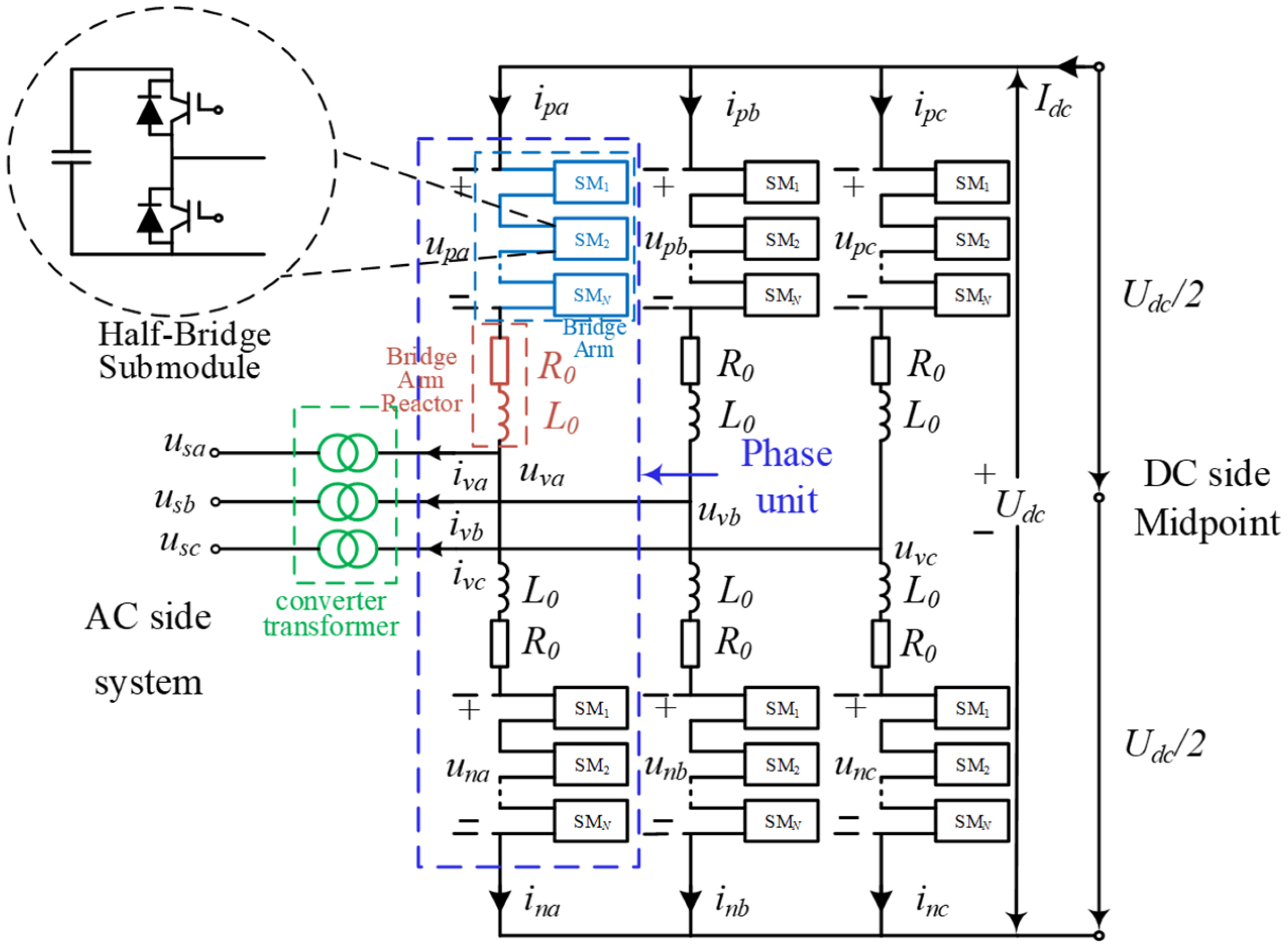
The flexible DC transmission system has a two-terminal MMC–HVDC structure. The topology of a single-side MMC is shown in Figure 1. Taking the system shown in Figure 1 as an example, the mathematical model of MMC is as follows [16,17]:
where , is the differential-mode voltage of the upper and lower arms, is the common-mode voltage of the upper and lower arms, is the circulating current of the j-phase arm, and is the phase current of the j phase.
Figure 1.
Main circuit of MMC in MMC-HVDC converter station.
As can be seen from Formula (1), when the DC voltage and the AC-side voltage remain unchanged, by controlling the differential-mode voltage and the common-mode voltage, the current and circulating current output by the converter can be controlled. This is the basic idea of MMC control.
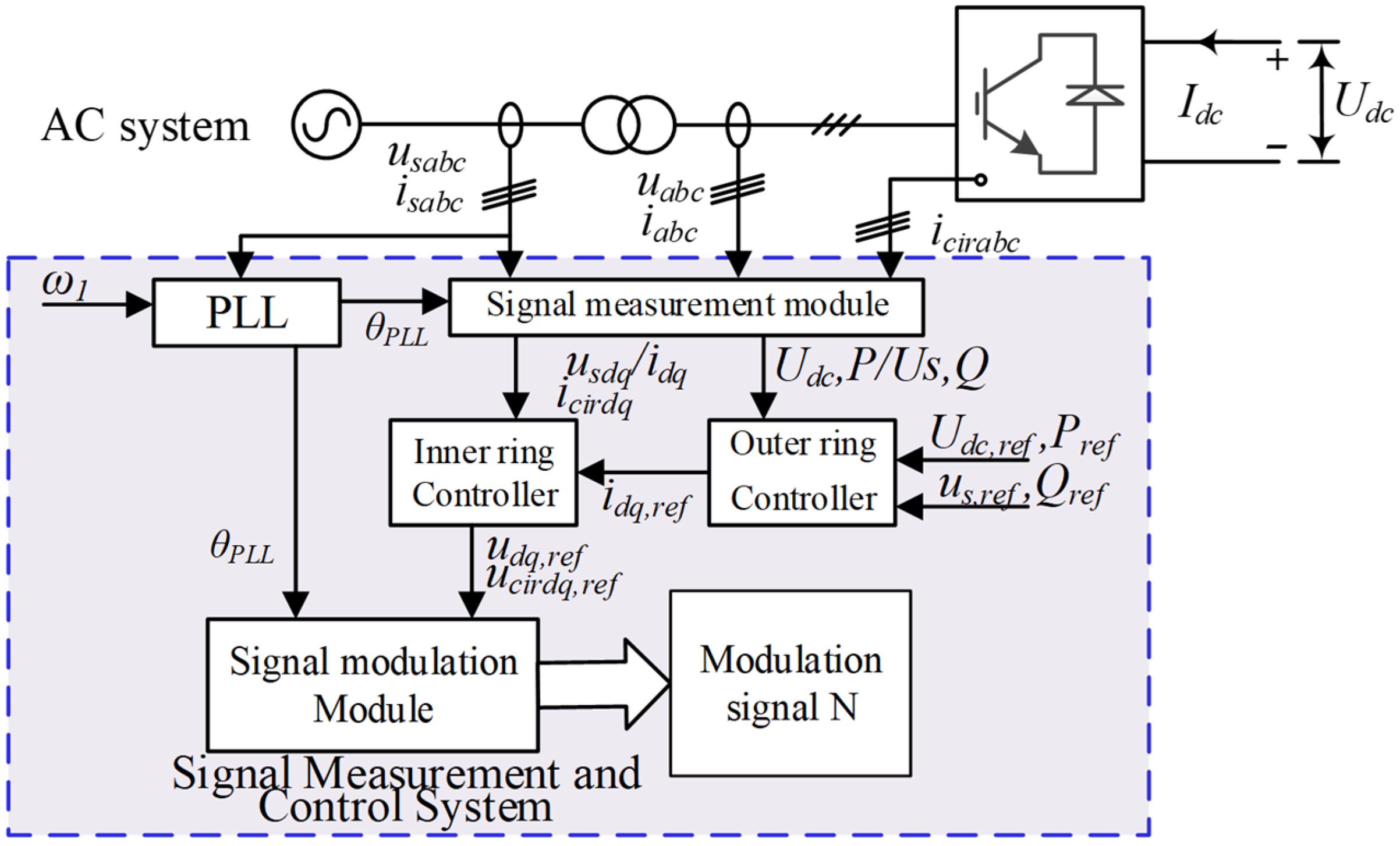
The MMC control system mainly consists of main links such as a phase-locked loop (PLL), an outer-loop controller, an inner-loop controller, and a circulating-current controller (CCSC). Figure 2 shows the block diagram of the MMC control system.
Figure 2.
MMC control diagram.
In Figure 2, , , , are the actual values of the DC voltage, AC bus voltage, active power, and reactive power, respectively; , , , are the reference values of the DC voltage, AC bus voltage, active power, and reactive power, respectively; , , , are the reference values of the d, q-axis current and voltage output by the inner and outer loop controls, respectively; , , , are the d- and q-axis components of the AC current and voltage, respectively; is the fundamental angular velocity of the voltage; , are the d- and q-axis components of the circulating current, respectively; , are the reference values of the d- and q-axis voltage generated by the circulating current control, respectively.
According to the MMC model shown in Figure 1 and Figure 2, considering the influence of link delay and ignoring the internal dynamic characteristics of MMC, the equivalent model [18] of the high-frequency impedance on the AC side of MMC in the case of the outer loop of the active power and the outer loop of the DC voltage is obtained, where the high-frequency impedance on the AC side of MMC in the outer loop of the active power is shown in Equation (2), and the high-frequency impedance on the AC side of MMC in the outer loop of the DC voltage is shown in Equation (3).
where , , and are the transfer functions of the inner- and outer-loop proportional–integral controllers, respectively, and is the transfer function of the DC voltage outer-loop proportional–integral controller; is the system signal processing and output delay link; , are the current and voltage control link delay links, respectively, and is the transfer function of the DC voltage control link delay link; , are the fundamental voltage and current amplitudes, respectively; , where is the open-loop transfer function of the phase-locked loop; is the AC current phase angle; , are the steady-state currents of , , respectively; and is the steady-state current of . and are the equivalent resistance and inductance, respectively, and is the DC resistance.
Thus, the high-frequency oscillation impedance model of the flexible DC transmission system is obtained. Subsequently, based on this method, the flexible DC transmission system will be modeled and analyzed to further study its relevant characteristics that cause high-frequency oscillations.
2.2. High-Frequency Oscillation Mechanism of MMC-HVDC Transmission System
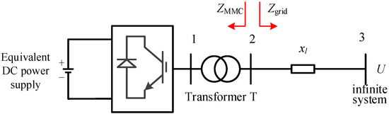
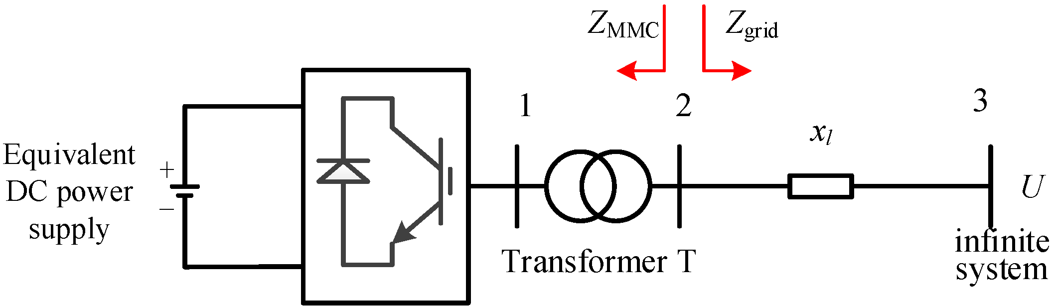
Taking the near-area power grid model of the single-ended flexible DC transmission system shown in Figure 3 as an example, the mechanism of high-frequency oscillations caused by the flexible DC transmission system is analyzed.
Figure 3.
Single-ended MMC-HVDC transmission system DC near-area power grid.
Assume that the grid impedance is and the converter equivalent impedance is . Then, according to the Nyquist stability criterion, if there is an intersection between and and the phase angle difference is greater than 180° (i.e., the phase margin is negative), resonance will occur at the corresponding frequency and the system will be unstable [18]. It can be seen that the high-frequency stability of the MMC-HVDC transmission system is jointly determined by the grid impedance and the MMC impedance. That is, the interaction between the MMC impedance and the grid impedance may cause high-frequency oscillations. Moreover, when the MMC system exhibits a “negative resistance-inductive” characteristic and the AC system exhibits a capacitive characteristic, high-frequency oscillations are likely to occur [18].
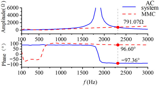
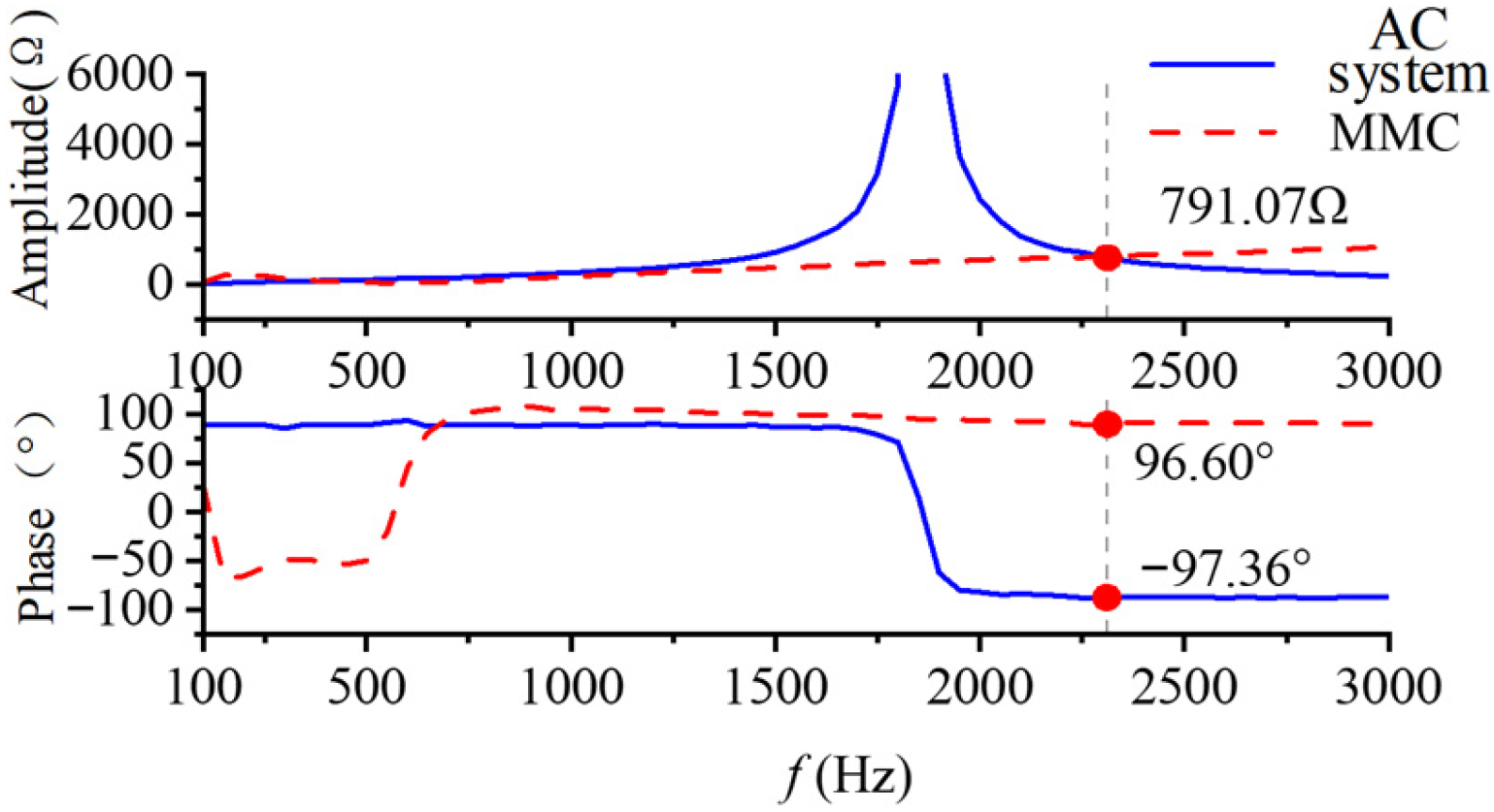
To conduct an intuitive analysis of the high-frequency oscillation mechanism, the equivalent impedance of the AC power grid and the equivalent impedance of the MMC AC side in the typical flexible DC transmission system shown in Figure 3 are obtained using Equation (2). Figure 4 presents the characteristic curves of the equivalent impedance of the AC power grid and the equivalent impedance of the MMC AC side in the single-terminal flexible DC transmission system.
Figure 4.
MMC and equivalent impedance of AC power grid.
It can be found from the analysis of Figure 4 that there is an intersection point between the equivalent impedance of the MMC and the equivalent impedance of the AC power grid at the frequency 2290 HZ, and the phase angle difference at this intersection point is greater than 180°. Therefore, according to the Nyquist criterion, high-frequency oscillation will occur in this single-terminal flexible DC transmission system at 2290 Hz. The oscillation frequency obtained from this analysis (2290 Hz) will serve as a typical frequency point for the quantitative analysis of the propagation characteristics of high-frequency oscillations in transmission lines and power grids in the subsequent chapters.
3. Response Characteristics of High-Frequency Oscillation System
3.1. Response Characteristics of Synchronous Generator to High-Frequency Disturbance
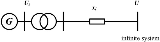
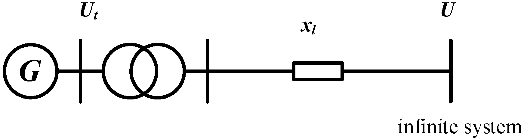
First, the high-frequency oscillation response mechanism of the synchronous generator is analyzed through a single-machine infinite-bus system. The system structure is shown in Figure 5, and the generator adopts a second-order classical model.
Figure 5.
Single-machine infinite-bus system diagram.
In the high-frequency oscillation analysis, it is assumed that the mechanical power of the generator is constant during the disturbance, and the continuous small periodic electromagnetic power disturbance induced in the power grid is .
Then, the linearized rotor motion equation is
where is the rotor angle deviation of the generator, is the fundamental frequency of the system, is the inertia time constant of the generator, is the damping coefficient of the generator, is the synchronous power coefficient of the generator, is the amplitude of the high-frequency disturbance, is the disturbance frequency, is the base frequency of the system, and .
Let , , , and ; then, Equation (4) can be written as
The solution of the second-order constant-coefficient linear non-homogeneous differential equation in Equation (5) is the total response of the system:
Only considering the steady-state oscillation process, and assuming that the steady-state solution of the rotor angle deviation is , we substitute it into Equation (4) to obtain the formula for the amplitude frequency characteristic of the rotor angle oscillation:
In the formula, , is the natural oscillation frequency of the system, and is the damping ratio.
An analysis of Equation (7) shows that, when ensuring the same change in the electromagnetic power of the generator for a specific synchronous generator, except for the disturbance frequency, the other parameters are all constants. Then, the amplitude of the rotor angle oscillation is a single-variable function of the oscillation frequency . When ensuring that the disturbance amplitude remains unchanged, within the frequency range of , the amplitude of the rotor angle oscillation gradually decreases as the disturbance frequency increases. The of the synchronous generator is generally 5~10 s, and, under normal output conditions, is 0.5~1. Then, the natural oscillation frequency is generally around 1 Hz, which is much smaller than the frequency range of high-frequency oscillations. Therefore, within the frequency range of high-frequency oscillations of 100 Hz~3000 Hz, the amplitude of the rotor angle oscillation gradually decreases as the disturbance frequency increases. Thus, the response characteristics of the generator’s high-frequency oscillation are obtained.
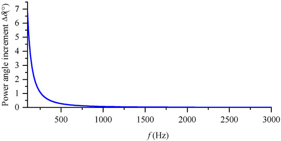
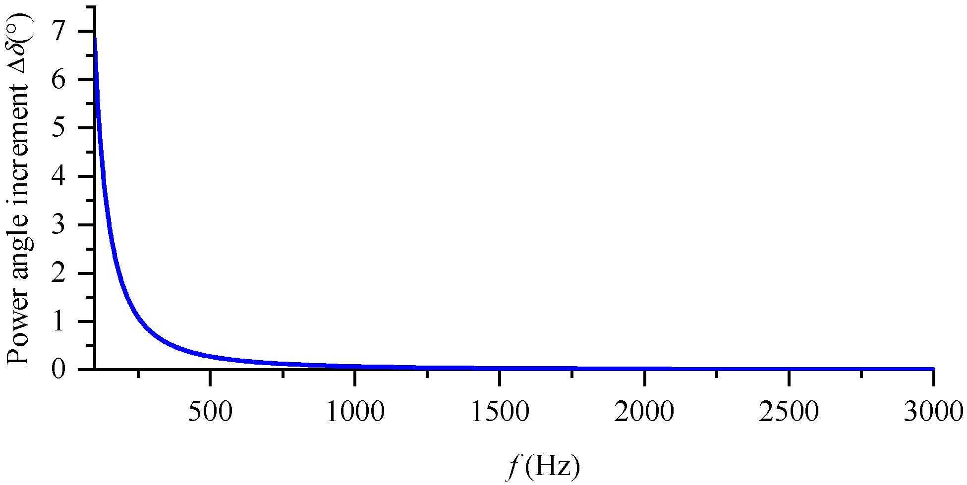
The above conducts theoretical derivation and analytical analysis on the high-frequency oscillation frequency characteristics of the synchronous generator. To further analyze its high-frequency oscillation characteristics, the high-frequency characteristics of a synchronous generator with specific parameters will be analyzed below. Let the inertia time constant be and the power angle during normal operation be 30°; . Without considering the damping effect, according to Equation (7), the curve of the rotor angle oscillation amplitude varying with the disturbance frequency, as shown in Figure 6, is obtained.
Figure 6.
Curve of frequency variation in rotor angle increment amplitude.
An analysis of Figure 6 shows that, within the frequency range of 100 Hz~300 Hz, when ensuring that the disturbance amplitude remains unchanged, the amplitude of the rotor angle oscillation gradually decreases as the disturbance frequency increases. As can be seen from Figure 6, when the disturbance frequency is 100 Hz, the amplitude of the rotor angle oscillation is 6.83°, while, when the disturbance frequency is 100 Hz, the amplitude of the rotor angle oscillation is 0.065°, and the difference in the response amplitude is nearly 100 times. It can be seen that the inertial effect of the synchronous generator rotor will filter out oscillations with higher disturbance frequencies. This characteristic indicates that, during high-frequency oscillations, synchronous generators primarily behave as impedance elements that passively absorb energy rather than as oscillation sources that actively emit high-frequency energy. This provides important theoretical support for the method proposed in this paper for locating oscillation sources based on high-frequency power flow (confirming that high-frequency power should flow from the oscillation source to the generator).
3.2. High-Frequency Oscillation Propagation Characteristics of Transmission Lines
For a long-distance transmission line with distributed parameters, let the length of the line be len and the resistance, inductance, and capacitance per unit length be r, l, and c, respectively. Then, the line can be represented by a length of len, characteristic impedance , and propagation constant .
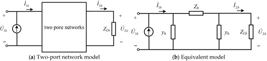
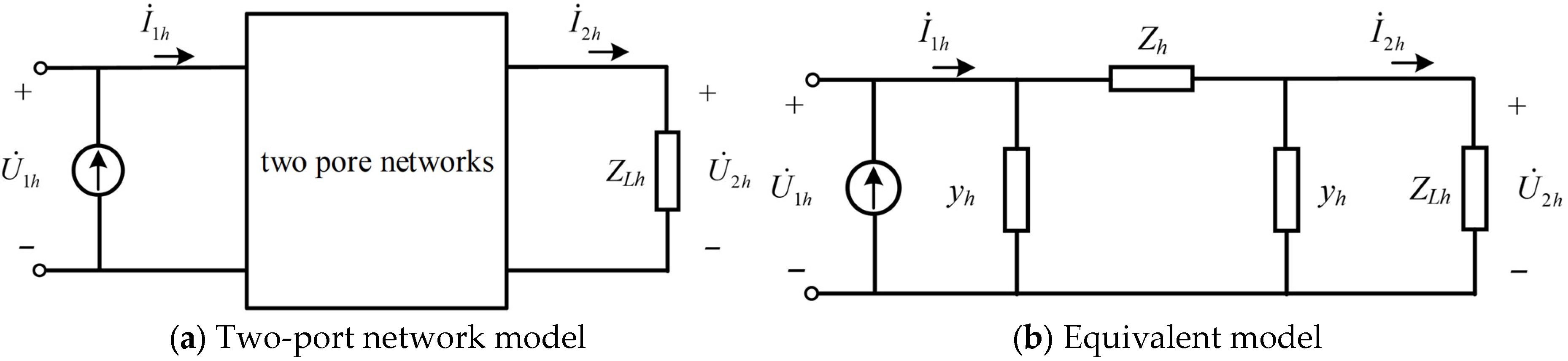
The transmission line is represented by the two-port network shown in Figure 7a:
where , , , and are the high-frequency oscillating voltage and oscillating current at the beginning and end of the line, respectively. The A, B, C, and D parameters are as follows:
Figure 7.
Distributed parameter transmission line model.
Combined with the analysis of Equations (9) and (10), the parameters , , and can represent the frequency characteristics of the transmission line.
Furthermore, the ABCD parameter model of the two-port network is represented by the accurate equivalent model shown in Figure 7b, and the parameters of the equivalent model are
Equation (11) is the equivalent model of the transmission line with distributed parameters. Next, based on the above model, the propagation characteristics of high-frequency oscillations in the transmission line with distributed parameters are analyzed. Let the high-frequency oscillating current injected from the beginning of the line be . After passing through a distance of len, the oscillating current reaches the end of the transmission line. The oscillating current at the end of the line is , and the load impedance at the end of the line is . Then, . From Equations (9) and (10), the propagation coefficient of the high-frequency oscillating current can be obtained as
Similarly, the propagation coefficient of the high-frequency voltage and the propagation coefficient of the high-frequency active power are
The amplitude of represents the amplitude characteristics of the high-frequency currents at the beginning and end, and the phase angle of represents the phase characteristics of the high-frequency currents at the beginning and end. It can be seen from Equation (12) that the factors affecting the high-frequency oscillating current coefficient are the resistance, inductance, capacitance, load impedance per unit length of the line, and line length. Therefore, whether the propagation of the high-frequency oscillating current in the line is an amplification effect or an attenuation effect mainly depends on the above five parameters.
The above has carried out a theoretical derivation of the frequency characteristics of the transmission line. Next, the five influencing factors will be analyzed separately, since the resistance, inductance, and capacitance per unit length of the line are the inherent parameters of the line and do not change with the operation mode of the system. Therefore, the influence of the load impedance and the line length on the high-frequency propagation characteristics of the transmission line is mainly considered. Let the rated voltage of the line be 230 KV, the fundamental frequency be 60 Hz, and the parameters of the transmission line be as follows: resistance r = 0.0529 (omhs/km), inductance l = 0.0014 (H/km), capacitance c = 0.0088 (uF/km), and line length len = 220 (km).
- (1)
- Analysis of the influencing factor of load impedance
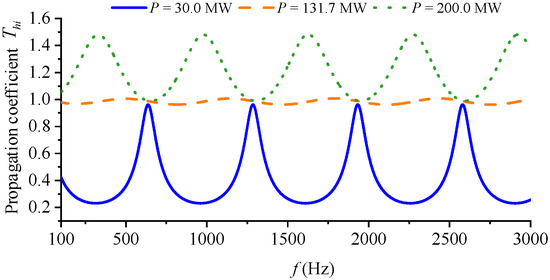
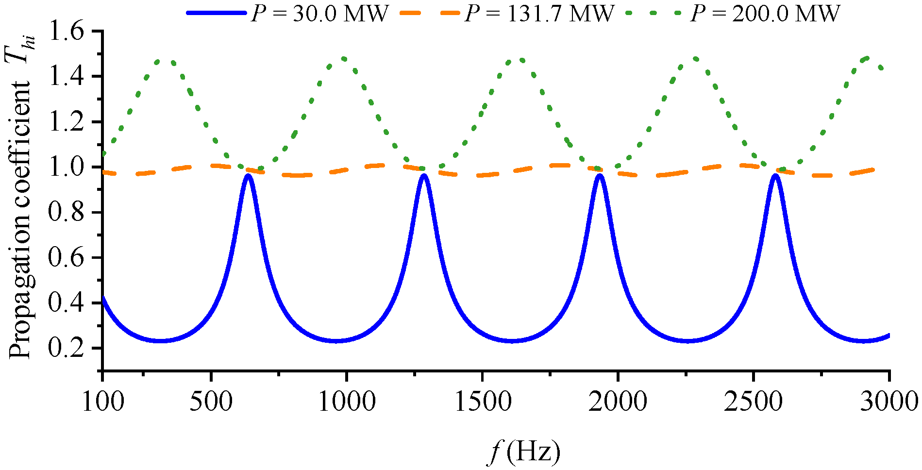
In the analysis process, it is assumed that the load impedance remains unchanged, that is, the frequency characteristics of the load impedance are ignored. Then, ; it can be seen that the load impedance is only related to the transmission power of the transmission line. On this basis, the analysis of the load impedance can be simplified to the analysis of the transmission power of the transmission line. According to the given transmission line parameters and rated voltage above, the natural transmission power of the transmission line is obtained as . Three operating conditions of the transmission line are set, and the reactive power transmitted by the line is . The active power transmitted by the line is set as , , and , respectively, and the influence of the change in the load impedance on the frequency characteristics of the high-frequency oscillation propagation coefficient is analyzed. The high-frequency oscillation propagation characteristics of the transmission line under different transmission powers are obtained using Formula (12), and the characteristic curve is shown in Figure 8.
Figure 8.
High-frequency current propagation coefficient of transmission lines.
It can be found from Figure 8 that the transmission power has a great influence on the high-frequency oscillation frequency characteristics of the transmission line. When the line is lightly loaded, the transmission line will have a large attenuation effect on the high-frequency current in a specific high-frequency band; when the transmission power of the line is the natural transmission power, the magnitudes of the high-frequency oscillation currents at the beginning and end are close; when the line is heavily loaded, the transmission line will amplify the high-frequency current.
- (2)
- Analysis of the influencing factor of line length
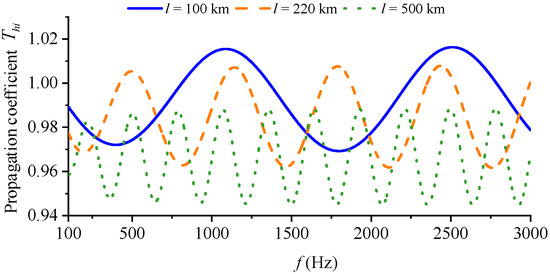
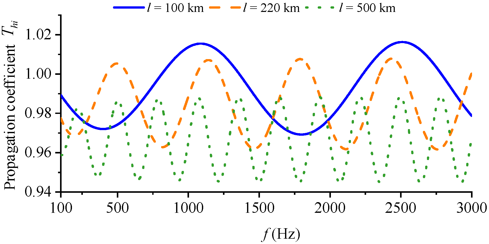
Set the transmission power of the transmission line near the natural transmission power, i.e., , change the length of the transmission line, and set the lengths of the transmission line to , , and , respectively. Analyze the influence of the change in the length of the transmission line on the frequency characteristics of the high-frequency oscillation propagation coefficient. Use Formula (12) to obtain the high-frequency oscillation propagation characteristics of the transmission line under different line lengths. Figure 9 shows the frequency characteristic curves of the high-frequency oscillation propagation of the transmission line under different line lengths.
Figure 9.
Transmission line high-frequency current propagation coefficient.
Through the analysis of Figure 9, the minimum value of the high-frequency current propagation coefficient appears when the line length is 500 km, and the maximum value of the high-frequency current propagation coefficient appears when the line length is 100 km. Moreover, the high-frequency current propagation coefficients in all three cases are near 1, and the difference between the maximum and minimum values is less than 0.06. It can be found that the influence of the line length on the high-frequency oscillation propagation characteristics of the transmission line is relatively small.
- (3)
- Propagation characteristics of high-frequency current, high-frequency voltage, and high-frequency active power
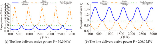
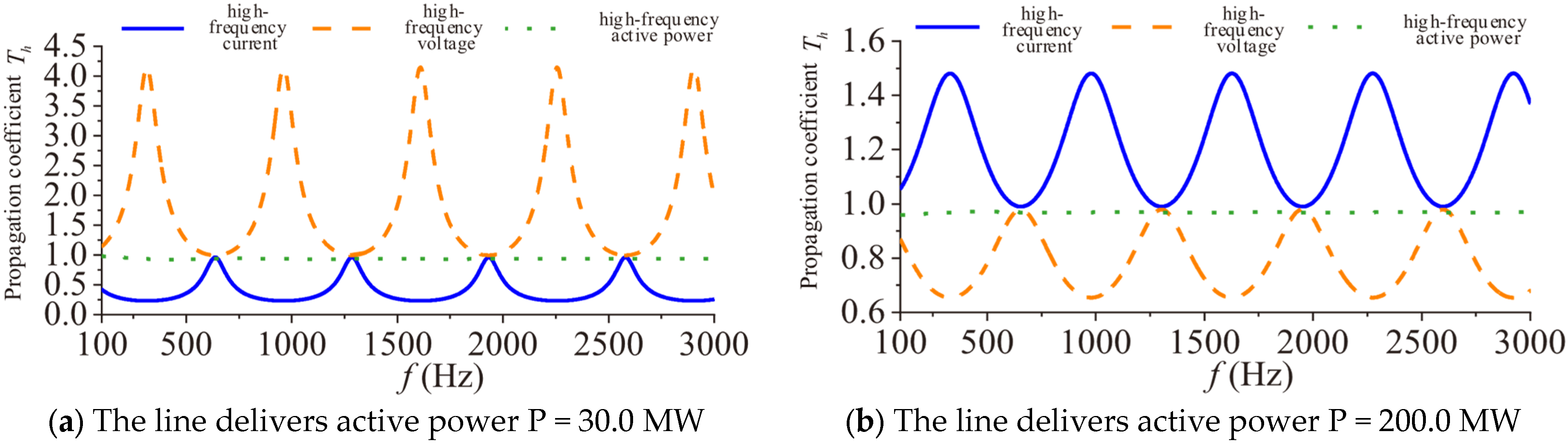
The above analyzes the two main factors affecting the propagation coefficient and finds that the change in the load impedance has a great influence on the propagation coefficient of high-frequency oscillation, while the change in the line length has a relatively small influence on the propagation coefficient of high-frequency oscillation. Next, continue to analyze the propagation characteristics of high-frequency current, high-frequency voltage, and high-frequency active power under different load impedances. Set the load powers to and , respectively, and use Equations (12)–(14) to analyze the propagation characteristics of high-frequency current, high-frequency voltage, and high-frequency active power, respectively. Figure 10 shows the propagation coefficient characteristic curves of the high-frequency current, high-frequency voltage, and high-frequency active power of the transmission line in the high-frequency band from 100 Hz to 3000 Hz.
Figure 10.
Comparison of propagation coefficients of high-frequency oscillation.
It can be found from the analysis of Figure 10a that, when the load power is low, the transmission line will amplify the high-frequency oscillating voltage and attenuate the high-frequency oscillating current; meanwhile, from the analysis of Figure 10b, it can be seen that, when the load power is high, the transmission line will attenuate the high-frequency oscillating voltage and amplify the high-frequency oscillating current. For the high-frequency active power, whether the load power is low or high, there is no obvious attenuation or amplification effect. At the same time, it can be found that the propagation coefficient of the high-frequency active power is not exactly equal to 1 but slightly less than 1; that is, the high-frequency power at the end is slightly less than the high-frequency power at the head end, which is mainly due to the resistance loss of the transmission line. Based on the above analysis, due to the frequency characteristics of the transmission line, it will amplify or attenuate the high-frequency voltage and high-frequency current, but has no obvious attenuation or amplification effect on the high-frequency active power. From a physical perspective, the amplification and attenuation of high-frequency and originate from the standing wave effect caused by distributed inductance and capacitance. High-frequency electromagnetic waves reflect at the load end, creating local maxima and minima for voltage and current amplitudes along the line. According to the law of energy conservation, the active energy injected at the sending end must flow to the receiving end, regardless of how the local and amplitudes fluctuate. The phase angle difference automatically adjusts to maintain constant active power transfer. Therefore, active power is inherently much less sensitive to transmission line spatial resonances than voltage and current amplitudes.
When studying the propagation path, the high-frequency current and high-frequency voltage cannot separately characterize the propagation path of high-frequency oscillation in the system, but the high-frequency oscillating instantaneous power can be used to characterize the propagation path of high-frequency oscillation. However, it should be noted that, for extreme high-frequency oscillations, the skin effect will dramatically increase the equivalent series resistance and the active power will suffer severe attenuation, which may limit the effective tracking range of this method.
4. High-Frequency Oscillating Instantaneous Power
In the Section 3, the high-frequency oscillation propagation characteristics of the transmission line are analyzed, and the results show that the high-frequency oscillating instantaneous power can be used to characterize the propagation path of high-frequency oscillation. Next, the instantaneous power characteristics of high-frequency oscillation are analyzed to obtain the expression form of the grid instantaneous power under high-frequency oscillation conditions.
4.1. High-Frequency Oscillating Instantaneous Power Characteristics
To clearly define the high-frequency instantaneous active power, subsequent mathematical derivations are established under the following ideal assumptions: (1) the grid operates under balanced three-phase conditions; (2) one single target oscillation frequency is analyzed at a time; and (3) other background harmonics are neglected.
When high-frequency oscillation occurs in the system, the three-phase fundamental frequency voltage and high-frequency voltage at the PCC point of the system can be expressed as
Then, the instantaneous voltage at the PCC node of the system can be expressed as
Similarly, the instantaneous current of the branch can be expressed as
where are the amplitudes of the power frequency voltage and current; are the amplitudes of the high-frequency component voltage and current; are the initial phase angles of the power frequency voltage and current; and are the initial phase angles of the high-frequency component voltage and current.
Then, the three-phase instantaneous power considering high-frequency oscillation is
Note that, under the balanced three-phase assumption, the sum-frequency components and double-frequency components are mathematically canceled out during the three-phase summation. The detailed expansion and derivation steps are provided in Appendix B. It can be seen from Equation (19) that the three-phase instantaneous active power consists of four terms. The first term is the instantaneous active power generated by the power frequency voltage and current; the second and third terms are the power fluctuation amounts with a frequency of generated by the interaction between the power frequency quantity and the components of high-frequency oscillation; the fourth term is the active power generated by the components of high-frequency oscillation. The last three terms related to the high-frequency voltage and high-frequency current components are called the high-frequency oscillating instantaneous active power :
The high-frequency oscillating instantaneous active power consists of two parts: the DC component and the AC component. The first and second terms of Equation (20) represent the AC fluctuation power, which oscillates at the difference frequency . The DC component of the third term is called the high-frequency active power.
4.2. Analysis Method for the Propagation Path of High-Frequency Oscillations
Based on the propagation characteristics of high-frequency oscillations in transmission lines obtained in Section 3 and the expression form of high-frequency oscillating instantaneous power in Section 4.1, a relatively clear understanding of the propagation mechanism of high-frequency oscillations in the power grid has been achieved. The previous analysis results show that the high-frequency voltage and high-frequency current will be amplified or attenuated during the propagation in transmission lines, which will affect the judgment of the distribution of high-frequency oscillations in the power grid. Therefore, the high-frequency current and high-frequency voltage cannot individually characterize the propagation path of high-frequency oscillations in the system, while the high-frequency active power has no obvious attenuation or amplification effect, and the high-frequency active power can characterize the propagation path of high-frequency oscillations.
The high-frequency active power calculation formula is
where are the amplitude and phase of the high-frequency voltage, and are the amplitude and phase of the high-frequency current. It should be noted that, although the fundamental active power and the high-frequency active power are both DC components in mathematical form, they are physically decoupled.
Therefore, when studying the propagation path, the detailed step-by-step execution procedure method based on the high-frequency power distribution of the branch can be adopted:
- (1)
- Obtain the broadband measurement data of the system branches. Apply Prony analysis to accurately identify oscillation frequency and separate the specific high-frequency voltage phasor and current phasor from the full waveform, thereby filtering out the fundamental wave and other frequency interferences.
- (2)
- Calculate the high-frequency active power for each branch using Equation (21) to determine the power distribution and its flow direction. For network branches, the positive direction is defined as the power flow from the head node to the end node. For load branches, the positive direction is defined as the flow into the load.
- (3)
- Locate the fundamental source of the high-frequency oscillation by identifying the node with the maximum injected high-frequency power.
- (4)
- Predefine a significance threshold (e.g., ). A branch is considered a significant propagation path only if its absolute high-frequency active power is greater than or equal to , where is the total high-frequency power injected by the oscillation source.
- (5)
- Finally, map the identified significant branches onto the actual network topology using directed arrows to indicate the power flow direction, thereby visualizing the precise propagation path and influence range of the high-frequency oscillation.
5. Case Study
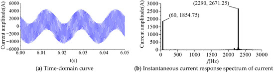
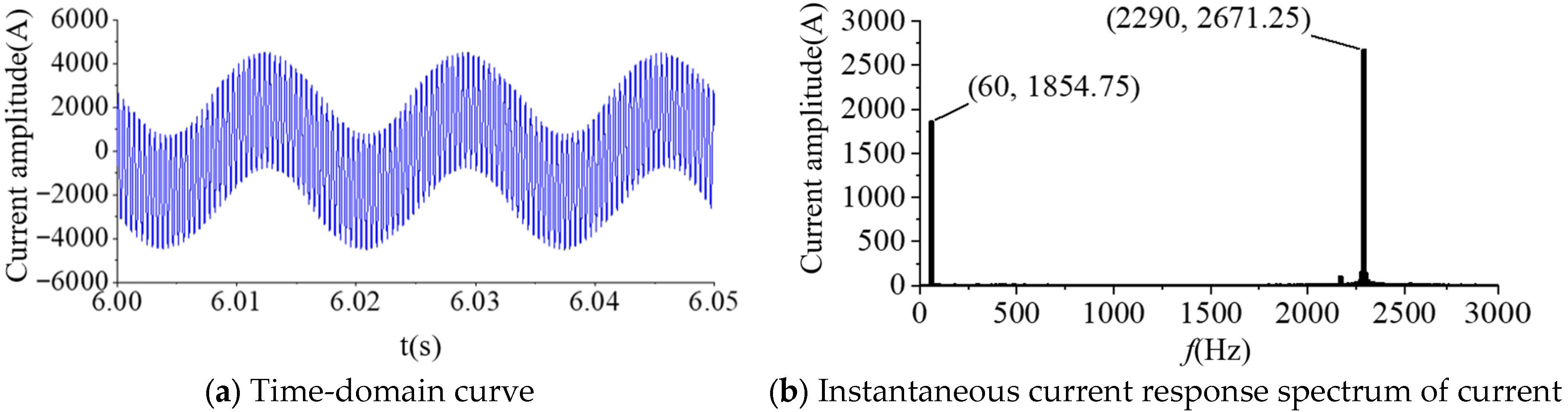
In order to obtain the high-frequency oscillation scene of the flexible HVDC transmission system, the following is based on Simulink to establish the near-area power grid model of the single-ended flexible HVDC transmission system shown in Figure 3. The DC side of the converter station is rated DC voltage, the DC side is connected to the equivalent DC power supply, the converter transmission power is 500 MW, and the converter transformer is connected to the infinite system through a 25 km distributed parameter transmission line. When the inner-loop current control parameter , the system will be excited by high-frequency oscillation at 2290 Hz and finally reach the stable state of high-frequency oscillation. The time-domain curve and amplitude spectrum of the converter-side current are shown in Figure 11.
Figure 11.
Inverter-side current oscillation mode.
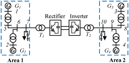
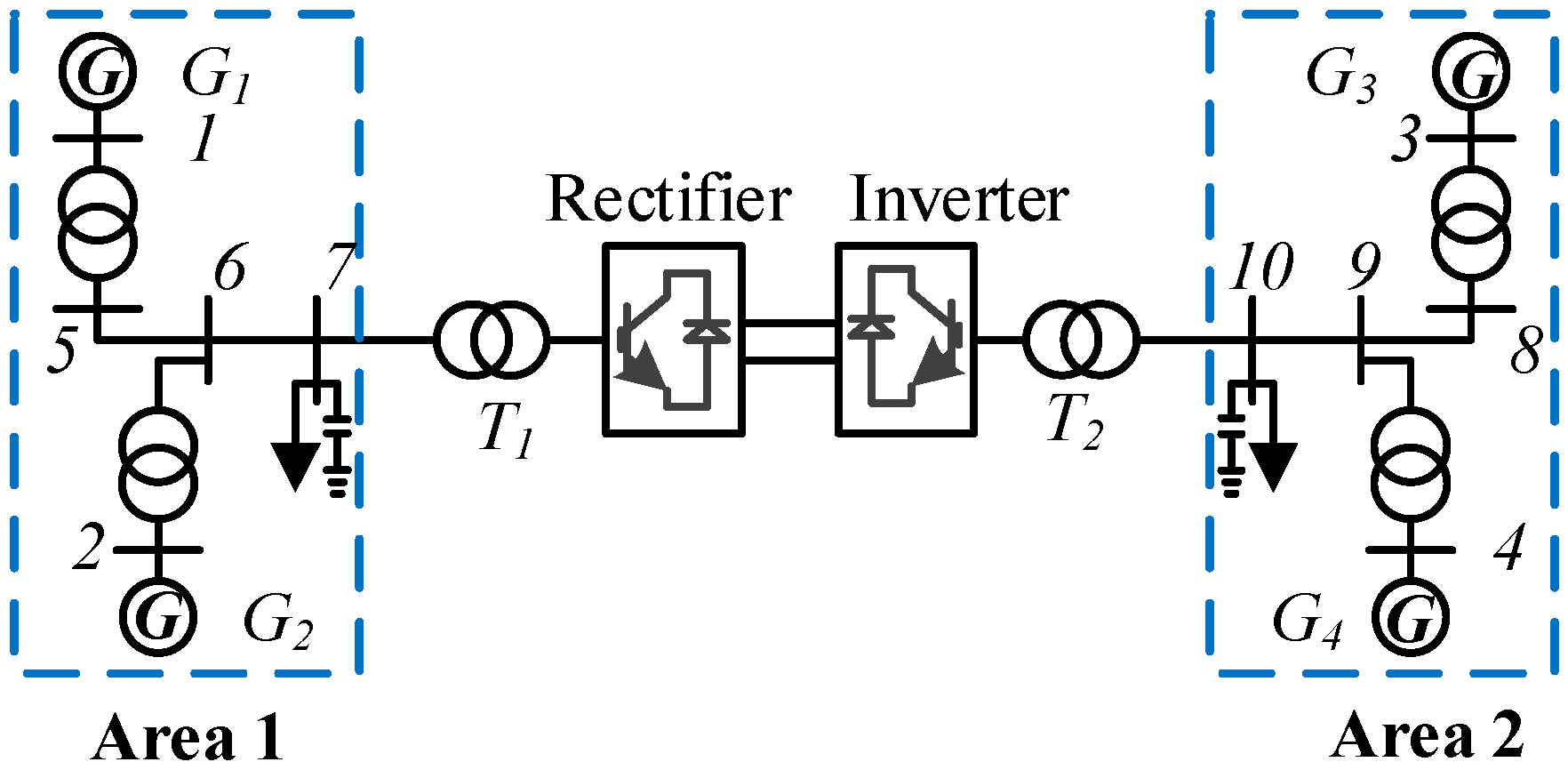
In order to further simulate the high-frequency oscillation caused by the actual flexible HVDC transmission system, a time-domain simulation model of the four-machine two-area MMC interconnected system is established in Simulink. The system structure is shown in Figure 12. The simulation model adopts the control mode commonly used in the active interconnection system at both ends. The rectifier side adopts constant DC voltage control and constant reactive power control, and the inverter side adopts constant active power and constant reactive power control.
Figure 12.
Four-machine two-area MMC-HVDC interconnection system.
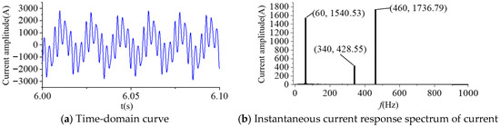
By changing the current inner-loop control parameter , the converter reaches a stable operating state after power adjustment. When t = 5 s, a 0.02 p.u. transmission power disturbance is added, and the system is excited at 340 Hz and 460 Hz. The high-frequency oscillation finally reaches a stable state of high-frequency oscillation. The waveform and spectrum of the A-phase current on the AC side of the converter are shown in Figure 13.
Figure 13.
Waveform of A-phase current of rectifier under high-frequency oscillation condition.
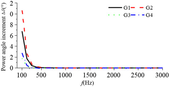
In Section 3.1, the high-frequency response characteristics of the synchronous generator are analyzed based on the single-machine system. In order to verify the universality of the above conclusions of the high-frequency oscillation response characteristics of the generator, the correctness of the analysis of the high-frequency oscillation response characteristics of the synchronous generator is verified in the four-machine two-area system. When the flexible DC system oscillates at a high frequency, the flexible DC system exhibits negative damping characteristics at a high frequency, so the flexible DC system can be equivalent to an AC oscillating current source. Since it is difficult to obtain the actual high-frequency disturbance data at each frequency under 100 Hz~3000 Hz, the response characteristics of high-frequency oscillation are studied by injecting high-frequency current at node 7. Figure 14 gives the power angle incremental response characteristics of four generators in a four-machine two-area system under high-frequency oscillation disturbances from 100 Hz to 3000 Hz.
Figure 14.
Four-machine two-area high-frequency oscillation response of generator.
From the analysis of Figure 14, it can be seen that the power angle oscillation amplitude of each generator decreases with the oscillation frequency of the system under the high-frequency oscillation disturbance of 100 Hz to 3000 Hz, which verifies the correctness of the high-frequency oscillation response characteristics of the synchronous generator. In addition, the order of the response amplitude of the four generators is ; this is consistent with the electrical distance between node 7 and each generator.
The following will use the two typical high-frequency oscillation modes of 2290 Hz and 460 Hz obtained by the previous simulation to analyze the propagation path of high-frequency oscillation. For the convenience of analysis, the propagation path of high-frequency oscillation is studied by injecting high-frequency current into the node.
5.1. Discussion on Practical Implementation and Sensitivity
5.1.1. PMU Bandwidth Limits and Time Synchronization Errors
Since our research targets high-frequency oscillations up to 3000 Hz, conventional PMUs (typically reporting at 50/100 frames per second) are insufficient due to bandwidth limits. Therefore, the proposed method relies on wide-frequency measurement systems. According to the Nyquist theorem, capturing a 3000 Hz signal requires a sampling rate of at least 6 kHz. In modern substations, wide-frequency measurement systems generally support sampling rates of 10 kHz or even higher (e.g., 20 kHz) [19], which provides sufficient bandwidth and resolution to extract high-frequency phasors without aliasing.
The calculation of high-frequency active power strictly requires synchronized voltage and current phasors. Modern substations utilize GPS or IRIG-B timing, with synchronization errors typically within . For an extreme high-frequency oscillation of 3000 Hz (period ), a timing error translates to a phase angle error of approximately . This marginal phase shift has a negligible impact on the calculation of active power magnitude and its directional flow, confirming the robustness of the method under standard hardware synchronization limits.
5.1.2. Measurement Noise and Window Length
The Prony method is used in our paper to extract specific oscillation frequencies. While Prony is sensitive to background noise, this sensitivity can be effectively mitigated by applying a bandpass filter before the extraction process. Regarding the window length, there is a fundamental trade-off: a longer window better filters out noise and increases frequency resolution but decreases the dynamic tracking speed. In practice, a window length containing two to five cycles of the lowest dominant oscillation frequency provides an optimal balance between accuracy under noise and dynamic responsiveness.
5.1.3. Multi-Tone Oscillations and Non-Stationary (Frequency Drift) Conditions
The proposed method performs excellently under multi-tone conditions. Unlike standard FFT, which suffers from spectral leakage, the Prony method can effectively distinguish multiple closely spaced frequency components. Once separated, Equation (21) is applied individually to each specific frequency component to calculate its respective high-frequency power propagation path. If the sources share the exact same frequency (e.g., ), the method will only display the net high-frequency power flow resulting from vector superposition. It cannot easily decouple the individual contribution capacity of each source without additional active perturbation techniques.
If the oscillation frequency drifts over time, the method remains valid by implementing a sliding-window algorithm (e.g., sliding-window Prony). By continuously updating the data window, the algorithm can track the transient variation in the oscillation frequency and dynamically compute the corresponding high-frequency power flow.
5.1.4. Performance Under Extreme Grid Conditions
While the proposed high-frequency instantaneous power is derived under idealized assumptions, its performance can be affected by complex non-ideal grid conditions. Specifically, under unbalanced faults, the emergence of negative-sequence components breaks the symmetry, introducing ripples into the fundamental power and causing cross-coupling with high-frequency components. In such cases, symmetrical component decomposition must be applied beforehand to strictly extract the positive-sequence quantities. Furthermore, extreme conditions like converter control saturation introduce severe non-linearities. This distorts the pure sinusoidal waveform, generating multiple harmonic sidebands () and causing the oscillation energy to leak across different frequency bands, which breaks the single-frequency assumption. Lastly, the presence of background interharmonics adjacent to the target oscillation frequency can induce a “beating effect” (low-frequency amplitude modulation). Consequently, the calculated high-frequency active power () will degrade from a stable DC value into a fluctuating low-frequency signal, making steady path identification challenging.
5.2. Analysis of the Propagation Path of High-Frequency Oscillations in a Four-Machine Two-Area System
(1) Scenario 1: The system undergoes high-frequency oscillations of 460 Hz
A high-frequency disturbance source is set at node 7, the amplitude of the high-frequency oscillation current is 1000 A, and the frequency is 460 Hz. According to Equation (21), the high-frequency oscillation power injected by the oscillation source node is calculated to be 6,916,364.57 W. The high-frequency powers of all network branches and load branches are presented in Table 1 and Table 2, respectively.
Table 1.
Four-machine two-area high-frequency power of network branch.
Table 2.
Four-machine two-area high-frequency power of load branch.
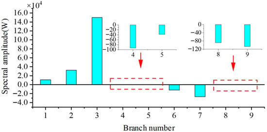
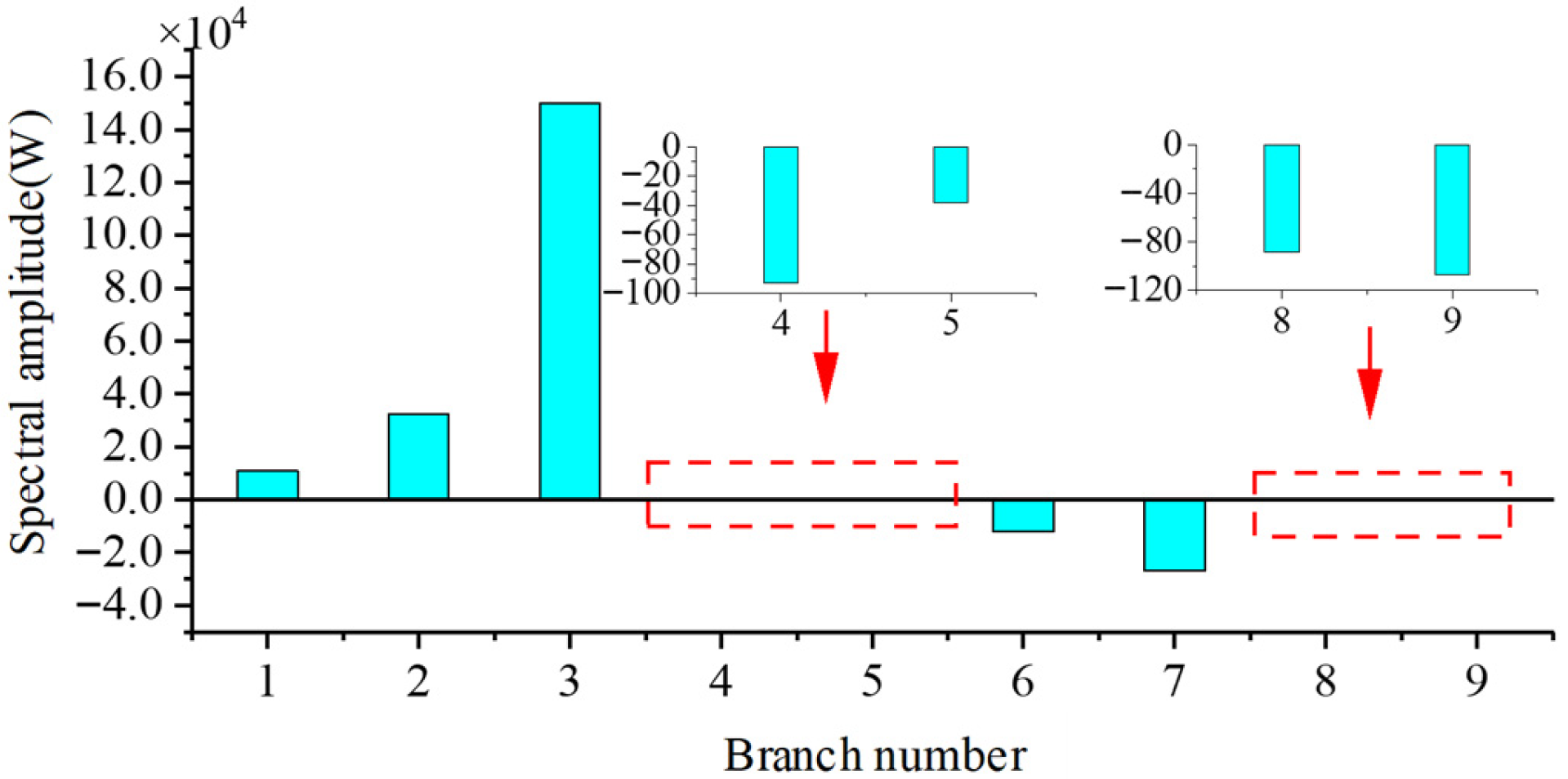
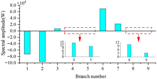
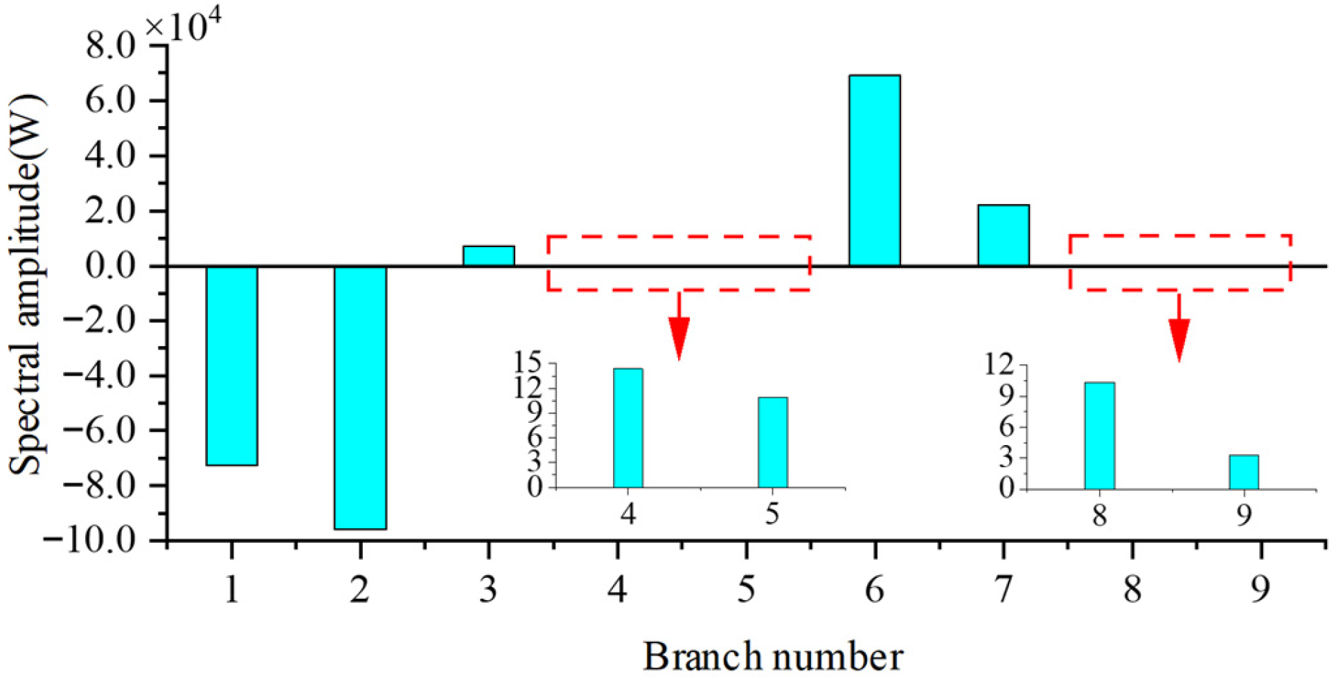
The high-frequency power of each network branch is shown in Figure 15. The positive direction of the network branch is from the head node to the end node, and the positive direction of the load branch is the current flowing into the load.
Figure 15.
Four-machine two-area 460 Hz branch high-frequency power distribution.
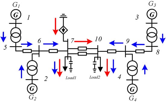
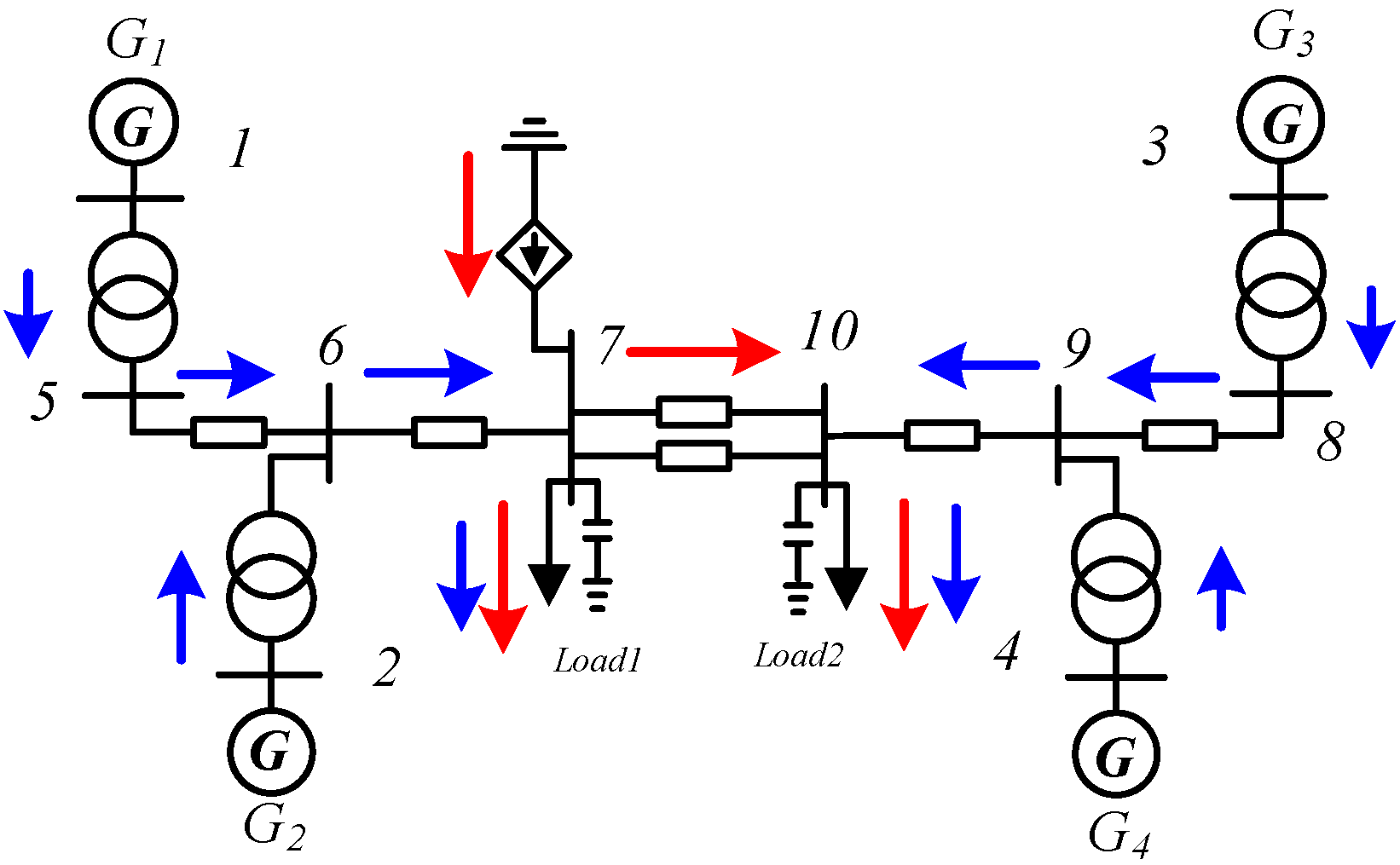
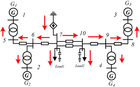
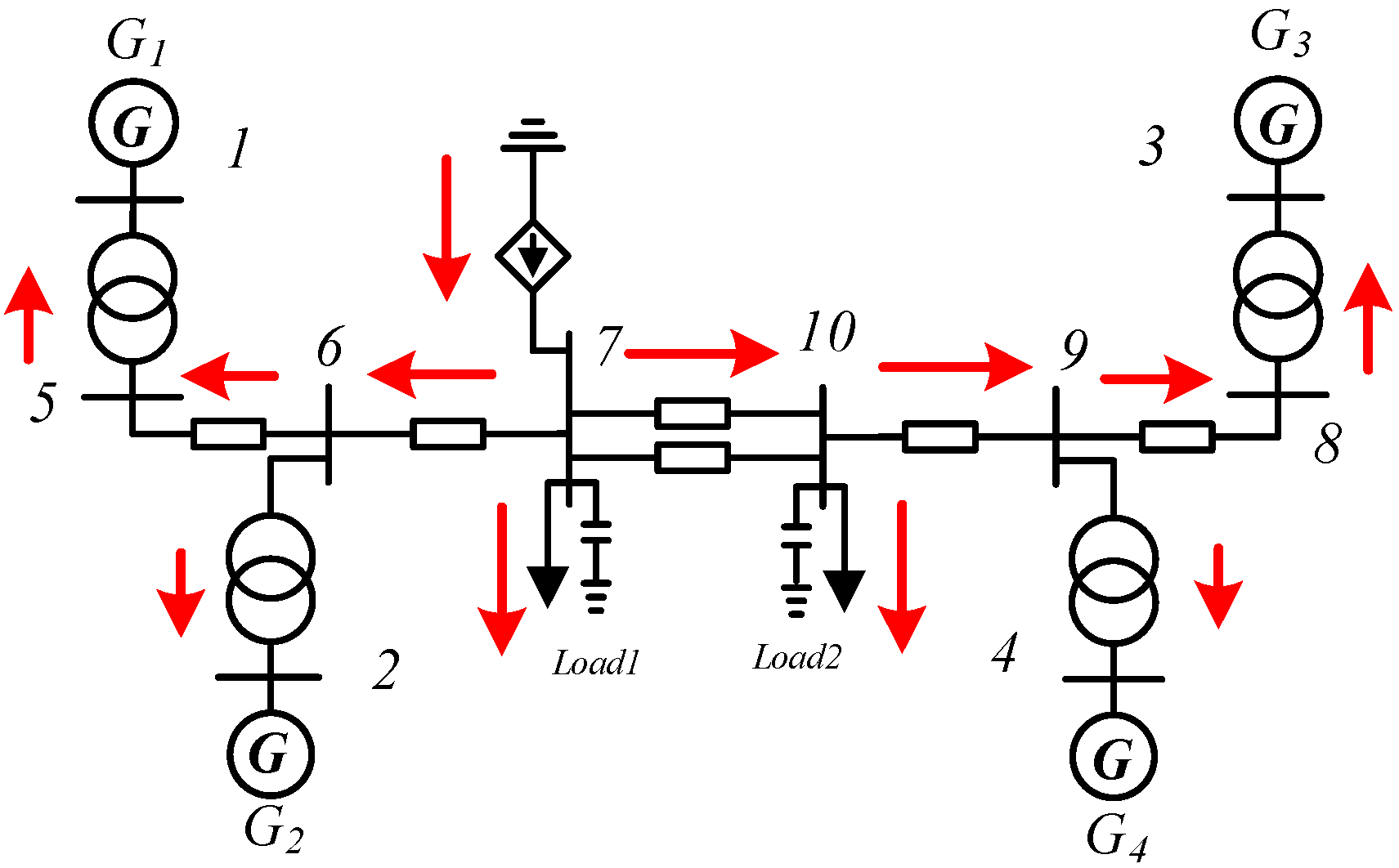
To clearly show the distribution of high-frequency oscillation power in the network, Figure 15 presents the oscillation power distribution of the four-machine two-area system, and the propagation path of high-frequency oscillations in the system obtained according to the branch power distribution is shown in Figure 16.
Figure 16.
Four-machine two-area 460 Hz high-frequency oscillation propagation path display.
Analysis by combining Figure 15 and Figure 16 shows that, when high-frequency oscillations with a disturbance frequency of 460 Hz occur at node 7 in the network, the sources of high-frequency power propagating in the system are divided into two parts. One part is the high-frequency oscillation power injected by the oscillation source node, represented by the red arrow in Figure 16, which is the main source of high-frequency oscillation power in the system (accounting for 99.6%); the other part is the high-frequency oscillation power provided by each generator to the system, represented by the blue arrow in Figure 16. The order of the magnitudes of the high-frequency oscillation power amplitudes of each generator is . It can be seen that this order of magnitudes of the high-frequency power amplitudes is the same as the order of magnitudes of the generator response amplitudes in the four-machine two-area system, . It can be seen that, except for a part of the high-frequency power consumed when flowing through long-distance transmission lines, the remaining high-frequency power will ultimately flow into the load.
Based on the analysis results of the high-frequency oscillation responses of each generator in the four-machine two-area system in Section 3 within the full frequency range of (100 Hz~3000 Hz), and combined with the analysis of the propagation path of the 460 HZ high-frequency oscillation in this section, it can be seen that, when the disturbance frequency is in the mid-frequency range of 100 Hz~1000 Hz and the response of the synchronous generator cannot be ignored, the dynamic characteristics of the synchronous generator need to be considered. Due to the existence of the oscillation source, the generator rotor undergoes forced motion at the oscillation frequency, resulting in an unbalanced power for the rotor of each synchronous generator, causing a mechanical power response, and each synchronous generator provides high-frequency oscillation power to the system. However, since the high-frequency oscillation power injected by the oscillation source node (accounting for 99.6%) is much larger than the high-frequency oscillation power provided by each generator to the system (accounting for 0.4%), the high-frequency oscillation power provided by the dynamic characteristics of the synchronous generator does not affect the judgment of the position of the oscillation source.
(2) Scenario 2: High-frequency oscillations of 2290 Hz occur in the system
Considering oscillation Scenario 2, change the frequency of the high-frequency oscillation and set the amplitude of the high-frequency oscillation current of the oscillation source at node 7 to 1000 A and the frequency to 2290 Hz. Calculate the high-frequency oscillation power injected by the oscillation source node according to Equation (21) as 416,800.38 W; the high-frequency oscillation powers of the network branches are shown in Figure 17. The propagation path of high-frequency oscillation in the system obtained according to the branch power distribution is shown in Figure 18.
Figure 17.
Four-machine two-area 2290 Hz branch high-frequency power distribution.
Figure 18.
Four-Machine two-area 2290 Hz high-frequency oscillation propagation path display.
It can be analyzed from Figure 17 and Figure 18 that, when a high-frequency oscillation with a disturbance frequency of 2290 HZ occurs at node 7 in the network, the high-frequency oscillation power injected by the oscillation source node is the only source of high-frequency oscillation power in the system, which is represented by a red arrow in Figure 18. At the same time, it can be found that the high-frequency power flowing to Area 1 is greater than that flowing to Area 2. Except for a part of the high-frequency power being lost when flowing through long-distance transmission lines, the remaining high-frequency power will ultimately flow to load and generator nodes.
Based on the analysis results of the high-frequency oscillation responses of each generator in the four-machine two-area system within the full frequency band of (100 Hz~3000 Hz), and combined with the propagation path of 2290 Hz high-frequency oscillation in this section, it can be determined that, when the disturbance frequency is in the high-frequency band of 1000 Hz~3000 Hz, ignoring the dynamic response characteristics of synchronous generators, the generators are regarded as constant impedance models for analysis. Therefore, the oscillation source location can be determined by analyzing the high-frequency oscillation power distribution.
5.3. Analysis of High-Frequency Oscillation Propagation Path in New England 10-Machine 39-Node System
(1) Scenario 1: A high-frequency oscillation of 460 Hz occurred in the system
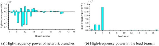
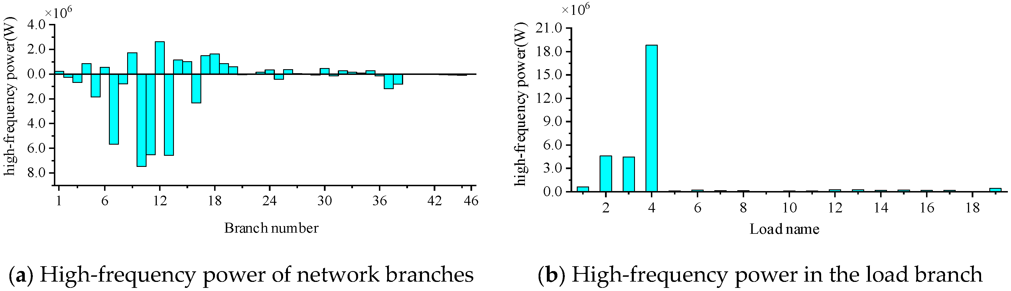
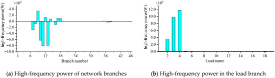
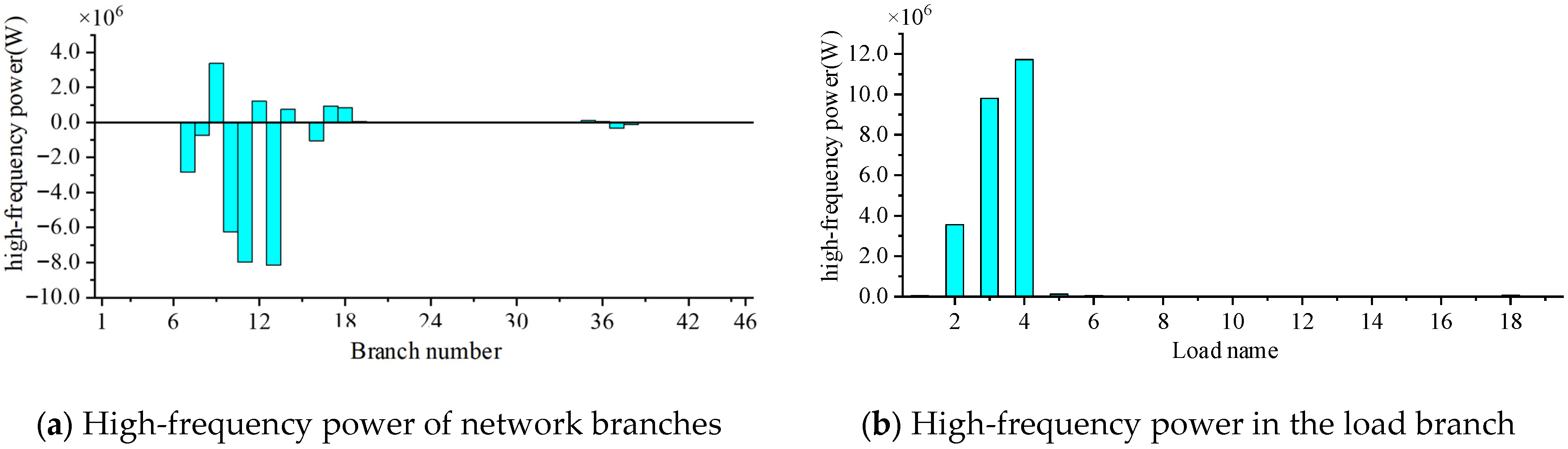
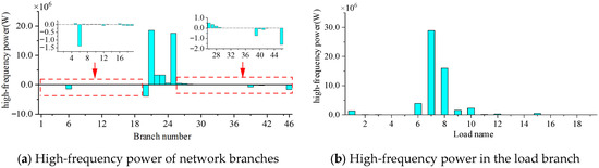
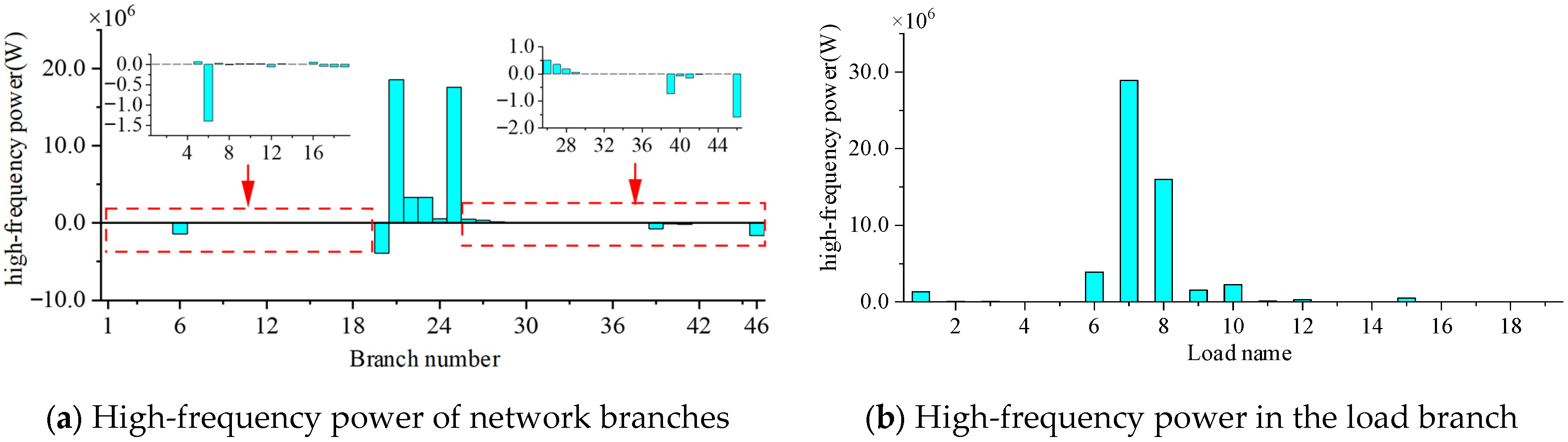
First, consider Oscillation Scenario 1. Set the amplitude of the high-frequency disturbance current at the oscillation source node of node 8 to be 500 A and the frequency to be 460 HZ. According to Equation (21), the high-frequency oscillation power injected by the oscillation source node is calculated to be 34,078,907.45 W. In the steady state of the oscillation, the high-frequency oscillation power of each network branch and load branch during the high-frequency disturbance at node 8 is shown in Figure 19. The corresponding nodes of branch numbers and loads for the 10-machine 39-bus system are shown in Table A1 in Appendix A.
Figure 19.
High-frequency power distribution when a 460 Hz disturbance is applied at node 8.
When a 460 HZ high-frequency disturbance is applied at node 8, it can be analyzed from Figure 19a that there is significant high-frequency power propagation near node 8. Among them, the high-frequency power passing through branch 10 is the largest, followed bybBranches 13, 11, and 7. At the same time, it can be found from the analysis of Figure 19b that the high-frequency power flowing into Load4 is the largest, followed by Load2, Load3, and Load1. Therefore, when there is a 460 HZ high-frequency disturbance at node 8, Load4, Load2, Load3, and Load1 are greatly affected by the oscillation. It can be seen that the high-frequency power is injected at node 8. After a part flows into Load4 at node 8, the paths with a relatively large distribution of the other part of the high-frequency power are as follows: most of it flows into Load3 at node 6 after passing through node 8–node 7–node 6, most of it flows into Load2 at node 4 after passing through node 8–node 5–node 4, and most of it flows into Load1 at node 39 after passing through node 8–node 9–node 39.
To rigorously validate the accuracy of the proposed method, the identified propagation paths are cross-verified with the network topology and the high-frequency electrical distances. In this simulation scenario, the exact disturbance injected at node 8 serves as the “ground truth”. At the high-frequency band, the line reactance () dominates the transmission impedance. The high-frequency power passing through branch 10 (from node 8 to node 5) is the largest among all connected branches. This outcome aligns with the topological reality: branch 10 possesses a lower equivalent high-frequency impedance (shorter electrical distance) compared to the alternative routes via node 9 or node 7. Similarly, the step-by-step attenuation of high-frequency power as it propagates deeper into the network (e.g., towards node 39 and Load1) exactly mirrors the cumulative increase in high-frequency path impedance. This correlation confirms that the proposed branch power distribution method is not merely generating numerical distributions but is accurately reflecting the physical laws of high-frequency energy propagation across the grid topology.
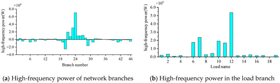
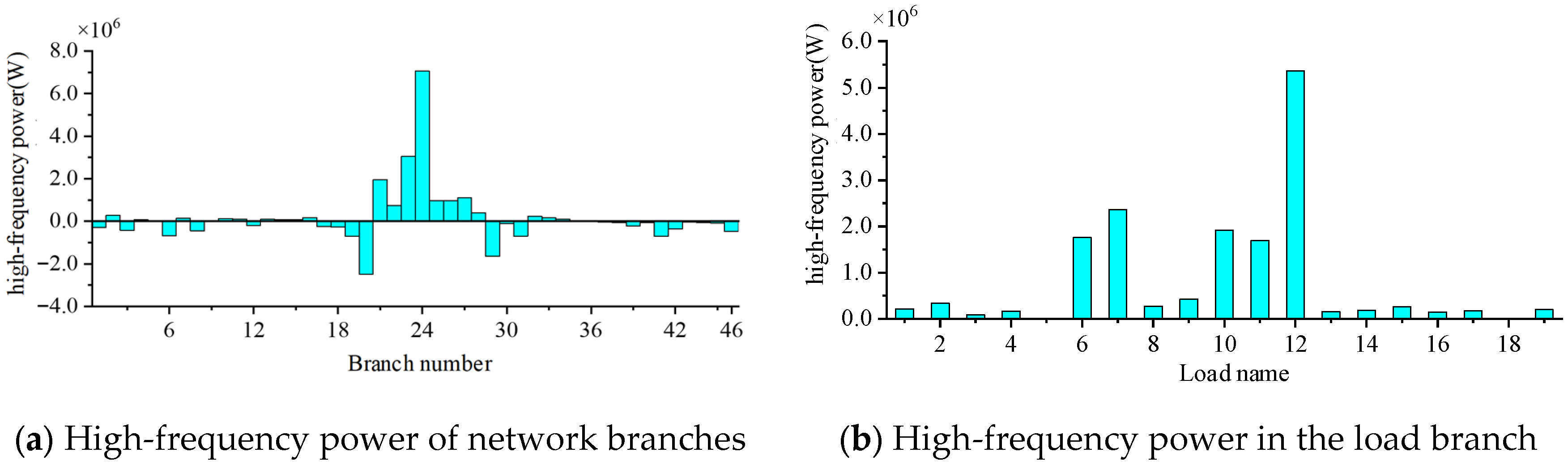
Set the amplitude of the high-frequency disturbance current of the oscillation source at node 16 to 500 A and the frequency to 460 HZ. Figure 20 shows the high-frequency power distribution diagrams of each branch in the system. It can be seen from Figure 20 that, when a 460 Hz high-frequency disturbance is applied at node 16, it can be found that there is significant high-frequency power propagation in branches 20, 21, …, 29, among which the high-frequency power of branch 24 is the largest; the high-frequency power at Loads 6, 7, 10, 11, and 12 is relatively large, and the high-frequency power at Load 12 is the largest. That is, the high-frequency oscillation power is injected at node 16 and propagates from node 16 to each branch of the system, and the loads near the oscillation source node are greatly affected by the oscillation. Figure 21 shows the oscillation propagation path of the entire network under this oscillation scenario.
Figure 20.
High-frequency power distribution when a 460 Hz disturbance is applied at node 16.
Figure 21.
Display of 460 Hz high-frequency oscillation propagation path in the New England 10-machine 39-node system.
(2) Scenario 2: A high-frequency oscillation of 2290 Hz occurred in the system
Set the amplitude of the high-frequency disturbance current of the oscillation source at node 8 to 500 A and the frequency to 2290 HZ. The high-frequency power of the 2290 HZ oscillation shown in Figure 22 is calculated according to Equation (21).
Figure 22.
High-frequency power distribution when a 2290 Hz disturbance is applied at node 8.
Set the amplitude of the high-frequency disturbance current of the oscillation source at node 16 to 500 A and the frequency to 2290 HZ. The analysis process is the same as above, and the high-frequency power distribution shown in Figure 23 is obtained.
Figure 23.
High-frequency power distribution when a 2290 Hz disturbance is applied at node 16.
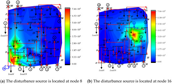
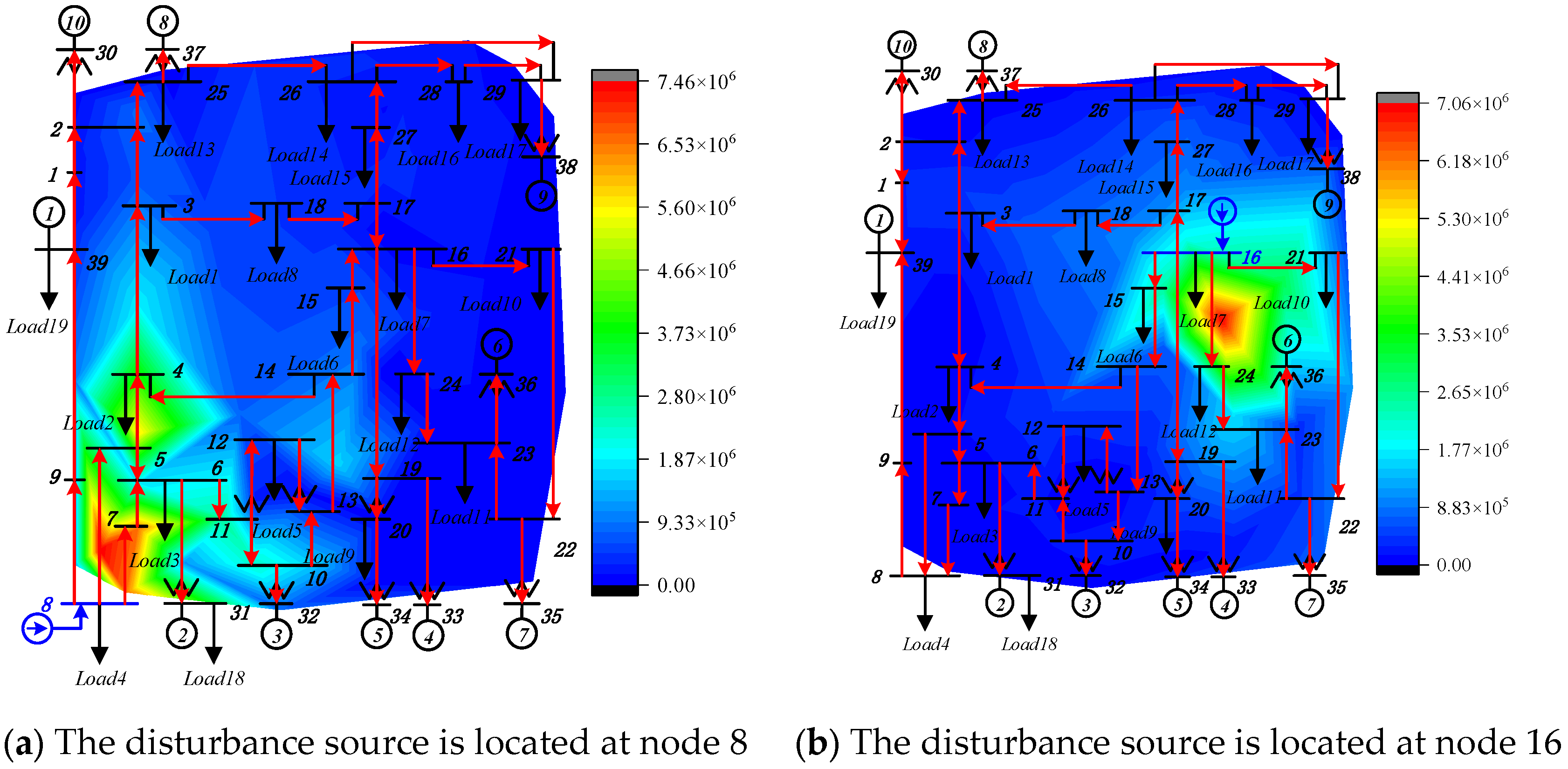
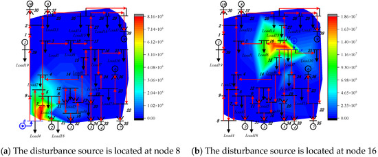
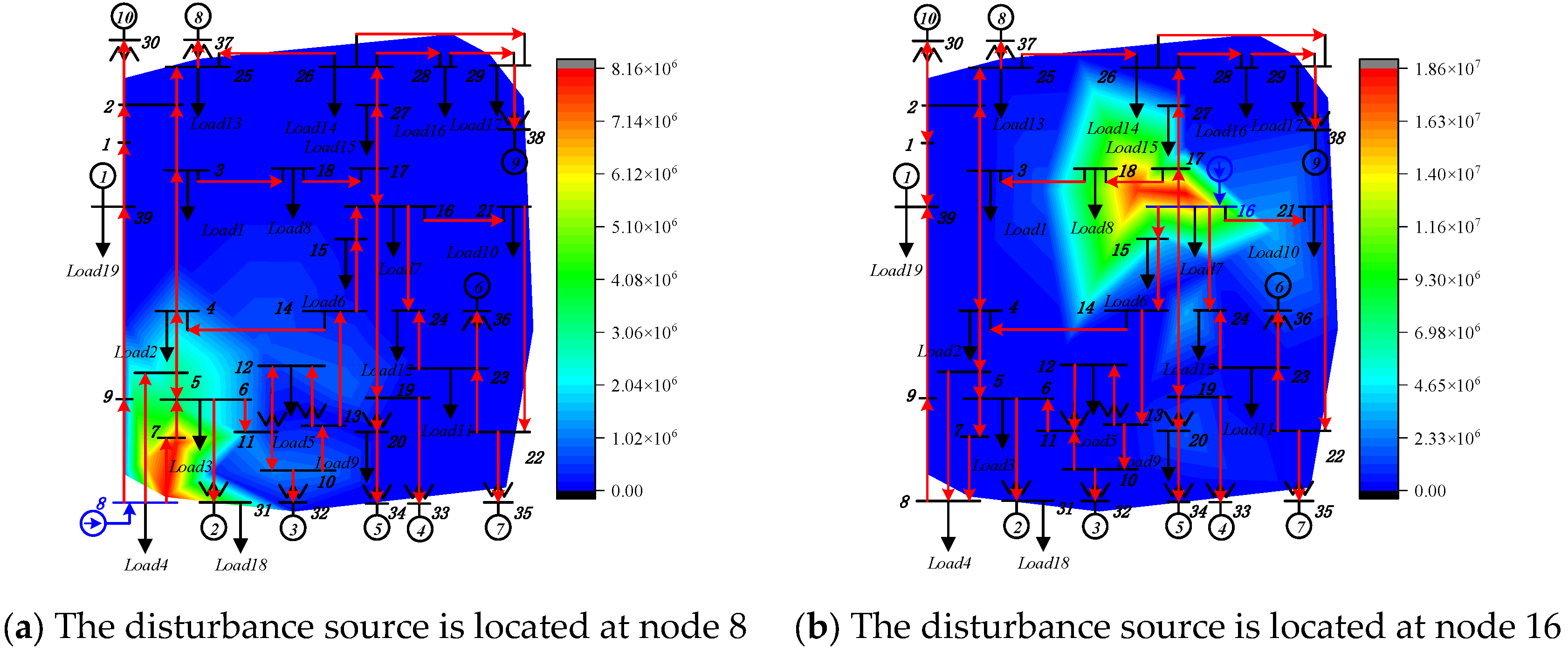
As can be seen from Figure 23a, the high-frequency power of branch 21 is the largest, and the high-frequency power of branch 25 is the second largest. That is, the power of the branch propagating from node 16 to node 17 is the largest, and then the main high-frequency oscillation propagates from node 17 to node 18. The oscillation propagation path of the entire network is shown in Figure 24. It can be seen from Figure 24a that, at the same node, oscillating currents with the same amplitude but different frequencies are injected. Through comparative analysis, it is found that the oscillation of 460 HZ spreads over a relatively wide range in the power grid, while the oscillation of 2290 HZ spreads over a smaller range in the power grid. Only in the branches near the oscillation source is there a large amount of high-frequency power propagation, and the high-frequency power in other branches is very small.
Figure 24.
Display of 2290 Hz high-frequency oscillation propagation path in the New England 10-machine 39-node system.
As can be seen from Figure 21a,b, when high-frequency oscillation occurs at node 8, the high-frequency power at node 8 is the largest, and the farther away from the oscillation source, the smaller the high-frequency power. Similarly, it can also be seen from Figure 24a,b that, when high-frequency oscillation occurs at node 16, the high-frequency power at node 16 is the largest, and the farther away from the oscillation source, the smaller the high-frequency power. It can be seen that the propagation path of high-frequency power can provide a basis for locating high-frequency oscillation sources.
According to the analysis of Figure 21 and Figure 24, when the system is at the same node and the disturbance amplitudes are the same, and when high-frequency oscillations of different frequencies occur, the propagation paths of the entire network are similar, but their main influence ranges may be different. In Figure 21b, the main influence range of the high-frequency oscillation of 460 HZ is near node 24, that is, the main influence range is in the lower left area of the disturbance source; meanwhile, in Figure 24b, the main influence range of the 2290 Hz high-frequency oscillation is near nodes 17 and 18, that is, the main influence range is in the upper right area of the disturbance source.
Compared with traditional oscillation localization methods such as Dissipating Energy Flow (DEF), modal energy flow, and impedance-based participation metrics, the proposed branch high-frequency power method not only identifies the source but also accurately maps the physical propagation path without being misled by line amplification/attenuation effects. A detailed comparison of these methodologies, including their required measurements, applicable scenarios, and pros/cons, is provided in Table A2 in Appendix A.
6. Conclusions
This paper focuses on the research of the propagation path problem of high-frequency oscillations caused by flexible DC transmission systems and studies the analysis method of high-frequency oscillation propagation paths based on broadband measurement data. The following conclusions are obtained:
- (1)
- The frequency response characteristics of the synchronous generator with high-frequency oscillation in the finite frequency band of 100 Hz~3000 Hz are analyzed from the mechanism, revealing that, within the frequency range of high-frequency oscillation of 100 Hz~3000 Hz, when the disturbance amplitude is constant, the response amplitude of the generator gradually decreases as the disturbance frequency increases. This result indicates that, under specific conditions, the high-frequency dynamic characteristics of the synchronous generator can be ignored, and it can be equivalent to an impedance model, effectively simplifying the high-frequency oscillation analysis process and providing a theoretical basis for the analysis of the high-frequency oscillation propagation path.
- (2)
- The high-frequency oscillation propagation characteristics of transmission lines are studied based on the distributed parameter line model. The influences of parameters such as load impedance and line length on the high-frequency oscillation propagation characteristics of transmission lines are analyzed in detail, and the propagation characteristics of the high-frequency oscillation current, voltage and high-frequency active power of transmission lines are analyzed.
- (3)
- The performance characteristics of the instantaneous power under high-frequency oscillation conditions are obtained. The proposed method for analyzing the propagation path of high-frequency oscillation based on the high-frequency power distribution of branches can accurately reflect the propagation path of high-frequency oscillation and the oscillation influence range in the actual system, and can provide a basis for locating the high-frequency oscillation source.
However, due to the complexity of the oscillation problem, there are deficiencies in the research on the high-frequency oscillation response characteristics of new energy power stations. To completely solve this problem, further in-depth research is still needed. Future research will focus on the following directions: (1) investigating the high-frequency dynamic response characteristics and coupling mechanisms of multiple interacting renewable energy stations (e.g., multi-infeed VSC-HVDC and wind farms); and (2) developing active damping and precise high-frequency suppression strategies guided by the identified physical propagation paths.
Author Contributions
Conceptualization, Y.L. and Y.H.; methodology, K.L.; software, Z.X.; validation, S.S., Y.Y. and Y.L.; formal analysis, Y.H.; investigation, K.L.; resources, Z.X.; data curation, S.S.; writing—original draft preparation, Y.L.; writing—review and editing, Y.Y.; visualization, Y.H.; supervision, Y.Y.; project administration, Z.X.; funding acquisition, Y.Y. All authors have read and agreed to the published version of the manuscript.
Funding
This research was funded by State Grid Shandong Electric Power Company Science and Technology Project grant number 52062624002L.
Data Availability Statement
The original contributions presented in this study are included in the article. Further inquiries can be directed to the corresponding author.
Conflicts of Interest
Authors Yudun Li, Yanqi Hou, and Zheng Xu were employed by State Grid Shandong Electric Power Co., Ltd. The remaining authors declare that the research was conducted in the absence of any commercial or financial relationships that could be construed as a potential conflict of interest. The authors declare that this study received funding from State Grid Shandong Electric Power Co., Ltd. The funder was involved in the study design, collection, analysis, interpretation of data, the writing of this article or the decision to submit it for publication.
Appendix A
Table A1.
The corresponding nodes of branch numbers and loads for the 10-machine 39-bus system.
Table A2.
Comparison of oscillation localization and propagation analysis methods.
Appendix B
Assume that both the fundamental () and the high-frequency () variables are balanced positive-sequence components. The instantaneous phase-A voltage and current can be expressed as the superposition of their fundamental and high-frequency components:
The instantaneous power for phase A is the product of its voltage and current, . Expanding this product and applying the trigonometric identity yields four sets of terms:
For a balanced three-phase system, the variables in phase B and phase C are shifted by and , respectively. The total three-phase instantaneous power is the sum of the three phases:
During this summation, a phase cancelation occurs:
Take the difference-frequency component of the second term () as an example. The initial phase of phase A is , the initial phase of phase B is , the initial phase of phase C is . These terms constructively add up to three times their single-phase magnitude.
For the sum-frequency terms and the double-frequency terms (,), the phase shifts accumulate. For instance, the sum-frequency phase shifts for phases A, B, and C become , , and . According to the identity , these terms perfectly cancel out to zero.
Consequently, all sum-frequency and double-frequency components are mathematically eliminated in the balanced three-phase summation. The final three-phase instantaneous power strictly consists of the following four terms:
References
- Ma, N.N.; Xie, X.R.; He, J.B.; Wang, H. Review of Wide-band Oscillation in Renewable and Power Electronics Highly Integrated Power Systems. Proc. CSEE 2020, 40, 4720–4732. [Google Scholar]
- Li, M.J.; Yu, Z.; Xu, T.; He, J.; Wang, C.; Xie, X.; Liu, C. Study on Complex Oscillation Problems Caused by Grid Connection Systems of New Energy Sources and Countermeasures. Power Syst. Technol. 2017, 41, 1035–1042. [Google Scholar]
- Irwin, G.D.; Jindal, A.K.; Isaacs, A.L. Sub-synchronous control interactions between type 3 wind turbines and series compensated AC transmission systems. In Proceedings of the 2011 IEEE Power and Energy Society General Meeting, Detroit, MI, USA, 24–28 July 2011. [Google Scholar]
- Guo, C.Y.; Peng, Y.; Xu, L.Q.; Yang, S.; Hu, Y. Analysis on High-frequency Oscillation Mechanism for MMC-HVDC System Considering Influence of Time Delay. Autom. Electr. Power Syst. 2020, 44, 119–126. [Google Scholar]
- Li, Y.F.; He, Z.Y.; Pang, H.; Yang, Y.; Ji, K.; Huang, W. High Frequency Stability Analysis and Suppression Strategy of MMC-HVDC Systems (Part I): Stability Analysis. Proc. CSEE 2021, 41, 5842–5856. [Google Scholar] [CrossRef]
- Lyu, J.; Zhang, X.; Cai, X.; Molinas, M. Harmonic state-space based small-signal impedance modeling of a modular multi-level converter with consideration of internal harmonic dynamics. IEEE Trans. Power Electron. 2019, 34, 2134–2148. [Google Scholar] [CrossRef] [Scilit]
- Xu, Z.G.; Li, B.B.; Han, L.J.; Hu, J.; Wang, S.; Zhang, S.; Xu, D.G. A complete HSS-based impedance model of MMC considering grid impedance coupling. IEEE Trans. Power Electron. 2020, 35, 12929–12948. [Google Scholar] [CrossRef] [Scilit]
- Feng, J.J.; Zou, C.Y.; Yang, S.F.; Zhao, X.; Fu, C.; Li, Y.; Xu, S.K. Accurate Impedance Modeling and Characteristic Analysis of VSC-HVDC System for Mid- and High-frequency Resonance Problems. Proc. CSEE 2020, 40, 4805–4820. [Google Scholar]
- Wang, X.; Liu, H.; Deng, X.Y. Mechanism Analysis and Risk Assessment of Broadband Resonance in Doubly-fed Induction Generator-based Wind Farms Integration Through Flexible HVDC. J. Glob. Energy Interconnect. 2020, 3, 238–247. [Google Scholar]
- Nian, H.; Zhu, M.W.; Xu, Y.Y. Modeling and Analysis of Frequency Coupling Characteristic for MMC Station Based on Harmonic Transfer Matrices. Autom. Electr. Power Syst. 2020, 44, 75–83. [Google Scholar]
- Li, G.H.; Wang, W.S.; Guo, J.B.; Chen, X.; Liu, C.; He, G.Q. Broadband Oscillation Mechanism and Analysis for Wind Farm Integration Through MMC-HVDC System. Proc. CSEE 2019, 39, 5281–5297+5575. [Google Scholar] [CrossRef]
- Li, Y.; Zou, C.Y.; Rao, H.; Xu, S.; Hong, C.; Huang, L.; Li, W. Resonance of VSC-HVDC with Extreme AC Grid. Proc. CSEE 2018, 38, 19–23. [Google Scholar]
- Huang, F.N.; Wei, C.; Zhou, J.; Liu, H.; Zhu, J.; Lin, L. MMC System High Frequency Resonance Based on Harmonic State Space Model. Power Syst. Technol. 2021, 45, 1967–1976. [Google Scholar]
- Dai, F.; Wang, G.; Zeng, D.H.; Hong, C.; Wu, W. Medium-& High-frequency Impedance Modeling and Resonance Mechanism Analysis of MMC-HVDC Transmission System. Power Syst. Technol. 2022, 46, 2356–2372. [Google Scholar]
- Li, Y.; An, T.; Zhang, D.; Pei, X.; Ji, K.; Tang, G. Analysis and Suppression Control of High Frequency Resonance for MMC-HVDC System. IEEE Trans. Power Deliv. 2021, 36, 3867–3881. [Google Scholar] [CrossRef] [Scilit]
- Tang, G.F. Voltage Source Converter Based High Voltage Direct Current Transmission Technology; China Electric Power Press: Beijing, China, 2010. [Google Scholar]
- Zhao, C.Y. Modeling and Simulation Technology of VSC-HVDC; China Electric Power Press: Beijing, China, 2014. [Google Scholar]
- Peng, Y.; Guo, C.Y.; Du, D.Y. Research on Medium and High Frequency Oscillation Suppression Approach Based on Impedance Tuning in Flexible HVDC System. Proc. CSEE 2022, 42, 8053–8063. [Google Scholar]
- Fan, C.; Yao, J.G.; Chang, N.C.; Su, D.; Wu, Y.; Dou, R. Discussion on Wide-frequency Measurement Technology for Power Electronized Power Grid. Autom. Electr. Power Syst. 2019, 43, 1–8+57. [Google Scholar]

Disclaimer/Publisher’s Note: The statements, opinions and data contained in all publications are solely those of the individual author(s) and contributor(s) and not of MDPI and/or the editor(s). MDPI and/or the editor(s) disclaim responsibility for any injury to people or property resulting from any ideas, methods, instructions or products referred to in the content. |
© 2026 by the authors. Licensee MDPI, Basel, Switzerland. This article is an open access article distributed under the terms and conditions of the Creative Commons Attribution (CC BY) license.