Conservation-Consistent Modeling of Time-Varying Transfer Delays with Applications in Energy Systems

Abstract

Time delays are intrinsic to energy systems, arising from transport phenomena, communication latency, and control dynamics; however, their accurate modeling remains challenging, particularly under variable operating conditions. The most common delays are constant over time and are easy to model and simulate. However, simulation tools of time-varying delay systems rely on signal-delay representations that fail to enforce conservation laws, leading to unphysical results in applications involving mass or energy transport. This study develops a physically consistent mathematical framework for time-varying transfer delays that explicitly couples kinematic evolution with conservation principles through a dynamic gain term. A systematic classification is introduced, distinguishing between signal delays (information transfer) and transfer delays (physical transport), further categorized by the source of variability in time delay into Types R (variable extraction), W (variable supply), and M (variable medium). The proposed formulation was implemented in Simulink through newly developed functional blocks supporting all delay variants and validated against representative heat transport scenarios. Comparative analysis demonstrates that standard signal-delay models violate energy conservation by generating spurious energy, whereas the proposed transfer-delay formulation preserves physical consistency under variable-flow conditions. The framework provides a rigorous foundation for accurate modeling of district heating networks, renewable energy integration with power-to-gas systems, thermal storage, and smart grid communications, supporting the development of reliable control strategies essential for the ongoing energy transition.

1. Introduction

1.1. Background and Motivation

Time delays are intrinsic features of numerous physical, biological, and engineering systems. They arise due to finite transmission, sensing, computation or actuation speeds; they fundamentally influence dynamic responses and control performance. Even small delays may degrade performance, induce oscillations, or destabilize an otherwise stable process [1,2]. Consequently, the analysis, modeling, and simulation of delayed systems remain a cornerstone in many scientific fields [3,4].

In modern energy systems, time delays play an increasingly critical role because of growing grid complexity, the integration of renewable energy sources (RES), and the widespread deployment of distributed energy resources (DER). The European Union’s Fit for 55 package and REPowerEU strategy require unprecedented levels of renewable penetration [5]. This transformation introduces challenges such as variable generation from solar and wind sources, response delays in energy storage, and latency in smart grid communication networks [6,7]. Accurate delay modeling is essential for grid stability, efficiency optimization and reliable operation of microgrids and virtual power plants [8,9]. The diversity of delay phenomena across different energy domains necessitates a unified mathematical framework capable of representing both information transmission and physical transport processes. Such a formulation is developed in Section 2.

Delays are prevalent across diverse scientific and engineering domains, including biomedicine [10,11,12,13,14,15] and process engineering [16,17,18]. However, this study specifically focuses on their critical implications for energy-related systems, where both physical and information delays strongly affect control and performance.

1.2. Mathematical Formulation of Delayed Systems

Classically, deterministic dynamical systems are described by ordinary differential equations (ODEs), in which the future trajectory depends solely on the current state and some inputs affecting the system. When delays are present, the system’s evolution also depends on past values. A general framework for such systems is provided by delay differential equations (DDEs):

$$\dot{x}\left(t\right)=f(x\left(t\right),x(t-\tau ),u\left(t\right)),$$

(1)

where $x\left(t\right)\in {\mathbb{R}}^n$ represents the system state vector, $u\left(t\right)\in {\mathbb{R}}^m$ the input vector, and f is a n-dimensional function describing the system dynamics. A special case of such systems is a case where time delay $\tau$ is a function of time; therefore, Equation (1) is being transformed into

$$\dot{x}\left(t\right)=f(x\left(t\right),x(t-\tau \left(t\right)),u\left(t\right)),$$

(2)

where $\tau \left(t\right)$ denotes a time-varying delay [19,20]. This functional dependence extends modeling capability and allows for more realistic representations of dynamic processes [21,22,23].

In the context of the transport delay examples developed in this study, the state and input are often scalar, implying $n=1$ and $m=1$, where $x\left(t\right)$ and $u\left(t\right)$ represent quantities such as mass flow rate [kg/s] or thermal power [W]. A physically important distinction exists between intensive quantities—such as temperature or concentration, which represent local thermodynamic states and are independent of system size—and extensive quantities, such as thermal power or mass flow rate, which scale with the amount of transported substance. As demonstrated in Section 5, this distinction has direct consequences for delay modeling: intensive quantities obey signal-delay representations, while extensive quantities require conservation-consistent transfer-delay formulations.

Delays arise in various forms across energy systems:

• Thermal systems: for example, heat-exchangers and thermal storage units display transport delays as energy propagates through fluid media [24,25,26,27].
• Electrical grids: communication-induced delays affect phasor measurement units (PMUs) and wide-area monitoring systems [28]; demand response programs exhibit lags between control signals and consumer reactions [29].
• Energy storage: batteries show electrochemical response delays during charge/ discharge cycles [30], and electrolyzers experience multiscale transport delays in hydrogen production [31,32].
• Renewables: photovoltaic systems experience measurement and actuation delays in maximum power point tracking (MPPT) algorithms [33,34], while wind turbines suffer from pitch control delays affecting power regulation [35].

From a numerical standpoint, simulating delayed systems poses additional challenges. Standard discretization schemes often fail to capture the infinite-dimensional nature of delay dynamics, which has motivated the development of dedicated solvers [19]. In software such as MATLAB/Simulink (version 2024b) delay elements are typically modeled via the Transport Delay block, limited to constant delays. Extensions to time-varying cases may lead to inaccuracies or numerical instabilities. To avoid confusion with Simulink-specific terminology, this study employs the more general concept of a transfer delay, encompassing both constant and time-varying cases.

1.3. Challenges and Research Gap

A variety of techniques have been proposed to approximate delays. Classical Padé-type expansions approximate constant delays in the frequency domain and are often used in control design [20]. Other approaches rely on spectral methods or discretization-based schemes, each involving trade-offs between accuracy and computational cost [19]. More advanced frameworks use switched-system theory or Lyapunov–Krasovskii functionals to derive stability conditions for hybrid systems with time-varying delays [36].

Despite these advances, the reliable simulation of time-varying transfer delays remains an open challenge—especially in industrial environments. In energy applications, inaccurate delay modeling can lead to

• Overestimation of renewable integration capacity [37];
• Suboptimal energy storage dispatch [38];
• Grid instability in microgrids with high DER penetration [8];
• Inefficient thermal management in district heating networks [25];
• Accelerated degradation of power electronics and batteries [30,39].

To address this gap, the present study introduces a simulation-based framework for transfer delays that enhances accuracy and physical consistency compared with standard modeling tools. Existing simulation environments—including Simulink’s Variable Transport Delay block—implement time-varying delays as pure signal shifts $y\left(t\right)=u(t-\tau (t\left)\right)$, which correctly adjust timing but systematically violate conservation laws for extensive quantities under variable-flow conditions, as demonstrated in Section 2. The novelty of the proposed framework lies in three contributions: (1) deriving a conservation-consistent formulation that couples kinematic delay evolution with a dynamic gain term $k\left(t\right)$, ensuring energy and mass balance; (2) establishing a systematic classification (Types R, W, M) based on which velocity component introduces time variability, enabling correct model selection for diverse applications; and (3) implementing these formulations as Simulink blocks that extend industrial simulation capabilities. The proposed approach enables unified and conservation-compliant modeling of thermal transport, power-to-gas conversion, phase-change storage, and distributed energy systems subject to communication-induced delays.

The remainder of this paper is structured as follows. Section 2 introduces the mathematical formulation of the proposed transfer delay, including illustrative examples and derivations. Section 3 presents a classification of variable delays. Section 4 discusses implementation aspects within the Simulink environment. Section 5 provides case studies related to heat transport in pipeline system. Section 6 concludes the paper and outlines directions for future research.

2. Motivation and Mathematical Formulation

This section presents representative examples that reveal inconsistencies in commonly employed models of time-varying delays and subsequently develops a physically consistent formulation of transfer delay. We will focus on a single time-varying delay element isolated from the overall system being modeled. The notation for this element used throughout is as follows: $u\left(t\right)$ denotes the input flow (such as mass flow [kg/s] or thermal power [W]), $y\left(t\right)$ denotes the output flow (also expressed in [kg/s] or [W]) and $\tau \left(t\right)$ is variable in time delay [s].

2.1. Motivation: Examples Revealing Model Inconsistencies

2.1.1. Crushing Process: Dimensional and Signal Inconsistency

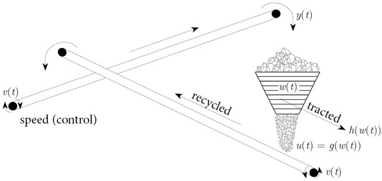
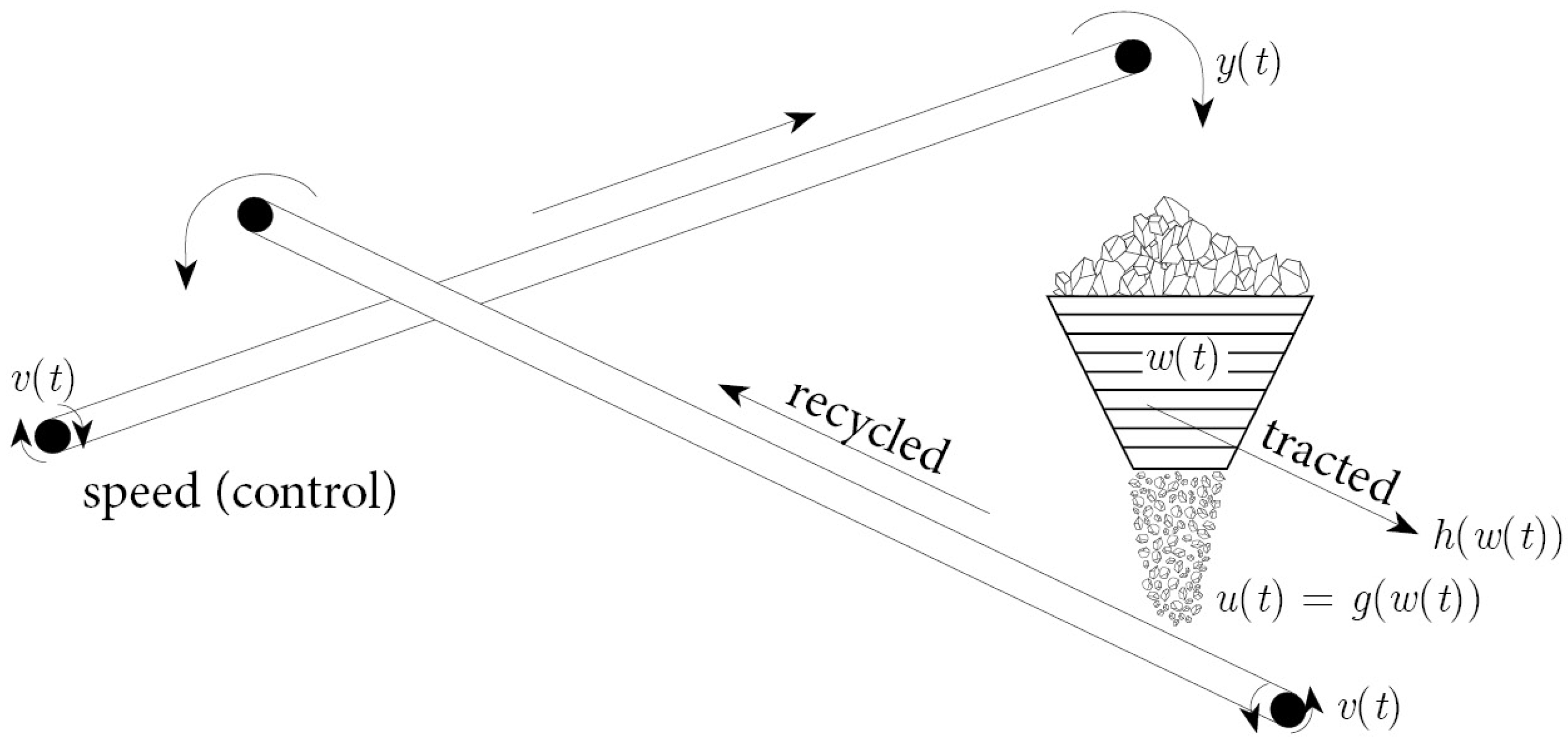
Richard [20] studied a conveyor-belt crushing process, in which material is transported and recycled into a mill, as illustrated in Figure 1. $w\left(t\right)$ is the mill mass [kg], $g(·)$ denotes the recycled flow function [kg/s], $v\left(t\right)$ the variable belt speed [m/s] and l the conveyor length [m]. This process has frequently served as a benchmark for time-varying delay modeling.

Figure 1. Crushing process with a conveyor belt (schematic illustration) used as a motivating example for time-varying delay analysis.

According to [20] input $u\left(t\right)$ and output $y\left(t\right)$ mass flows for the conveyor are expressed as $u\left(t\right)=g\left(w\right(t\left)\right)$ and $y\left(t\right)=g\left(w\right(t-lv\left(t\right))$, which gives the input–output description of the isolated conveyor:

$$\left\{\begin{array}{c}y\left(t\right)=u(t-\tau (t\left)\right),\hfill \\ \tau \left(t\right)=l·v\left(t\right).\hfill \end{array}\right.$$

(3)

However, as originally implied in [20], the delay $\tau \left(t\right)=l·v\left(t\right)$ is dimensionally inconsistent, with units of $[{\mathrm{m}}^2/\mathrm{s}]$. Therefore, a consistent formulation for $\tau \left(t\right)$ is

$$\tau \left(t\right)={\displaystyle \frac{l}{v\left(t\right)}},$$

(4)

which is properly expressed in $\left[{\displaystyle \frac{m}{m/s}}=s\right]$.

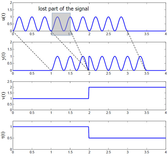
To verify this claim, a numerical simulation was conducted using Simulink with the corrected model (4). The input signal $u\left(t\right)$ was defined as a sinusoidal wave with unit amplitude and a period of 1 s, representing a time-varying mass flow rate. The conveyor length was fixed at $L=1$ m, and the transport velocity $v\left(t\right)$ was initially set to 1 m/s, then abruptly increased to 2 m/s at $t=2$ s, modeling a sudden change in conveyor belt speed. As shown in Figure 2, this velocity change causes the delay $\tau \left(t\right)$ to drop from 1 s to 0.5 s. The critical observation is that the output signal $y\left(t\right)$ exhibits a complete loss of a portion of the input waveform. Specifically, the shaded rectangular region in the top panel of Figure 2 highlights approximately half a period of the input signal that is completely lost in the output shown in the second panel. This missing fragment indicates that even the dimensionally corrected signal-shift model (4) fails to accurately represent physical transport processes under variable-velocity conditions.

Figure 2. Simulation of the dimensionally corrected but incomplete signal-shift model (4). Partial signal loss reveals violation of conservation principles.

2.1.2. Kinematic Analysis and Limitations of Simulink Transport Delay

Simulink provides two related blocks for modeling variable delays: the Variable Time Delay and Variable Transport Delay [40]. The first implements the basic input–output shift:

$$y\left(t\right)=u(t-t_d\left(t\right)),$$

(5)

where $t_d\left(t\right)$ is a prescribed delay [s]. The second aims to represent transport along a moving medium:

$$y\left(t\right)=u(t-{\tau }_d(L,v_m\left(t\right))),$$

(6)

where ${\tau }_d$ denotes the delay computed from the medium-length L and its velocity $v_m\left(t\right)$.

Zhang and Yeddanapudi [40] stated that many physical systems can be modeled with Variable Transport Delay blocks, such as conveyor belt systems and incompressible flow through a pipe (the outlet temperature modelled as a variable transport delay of inlet temperature). To verify whether Simulink’s Variable Transport Delay block can actually be used to model a conveyor belt, a second numerical experiment was performed. The simulation setup was identical to that described in Section 2.1.1. The Simulink Variable Transport Delay block was used to model the conveyor belt transport; see Figure 3. Indeed, now there is no problem with the lost part of the input signal, as in the previous example.

Figure 3. Simulation with standard Variable Transport Delay. The model satisfies the signal shift but violates the mass balance, demonstrating the necessity of the dynamic gain term $k\left(t\right)$.

However, the results presented in Figure 3 reveal violations of mass conservation. The output signal $y\left(t\right)$ exhibits signal distortion and amplitude reduction during and after the velocity transition, particularly visible in the interval $t\in [2,3.5]$ s where irregular oscillations appear. Quantitative analysis confirms a mass imbalance: the total input mass ($m_{in}=1.5$ kg) exceeds the total output mass ($m_{out}=1.25$ kg), indicating that approximately 17% of the transported mass is lost. This unphysical behavior demonstrates that the standard Variable Transport Delay block in the Matlab environment, despite its intended purpose for modeling physical transport, does not enforce conservation laws under variable-flow conditions.

The root cause of this deficiency is a category mismatch: the Variable Transport Delay block implements a signal-delay formulation appropriate for intensive quantities, such as temperature, but not for extensive quantities, such as thermal power or mass flow rate, which require amplitude scaling to satisfy conservation laws. This distinction motivates the framework developed in Section 2.

2.2. Signal Delay vs. Transfer Delay: Physical Distinction

Having exposed the limitations of existing formulations, this subsection establishes the physical distinction between a signal delay and a transfer delay.

In the case of a signal delay the quantity being delayed is purely informational, and input and output signals follow the equation:

$$y\left(t\right)=u(t-\tau (t\left)\right),$$

(7)

and do not necessarily obey the principles of conservation of mass or energy.

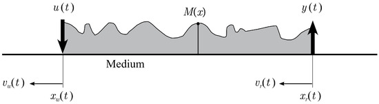
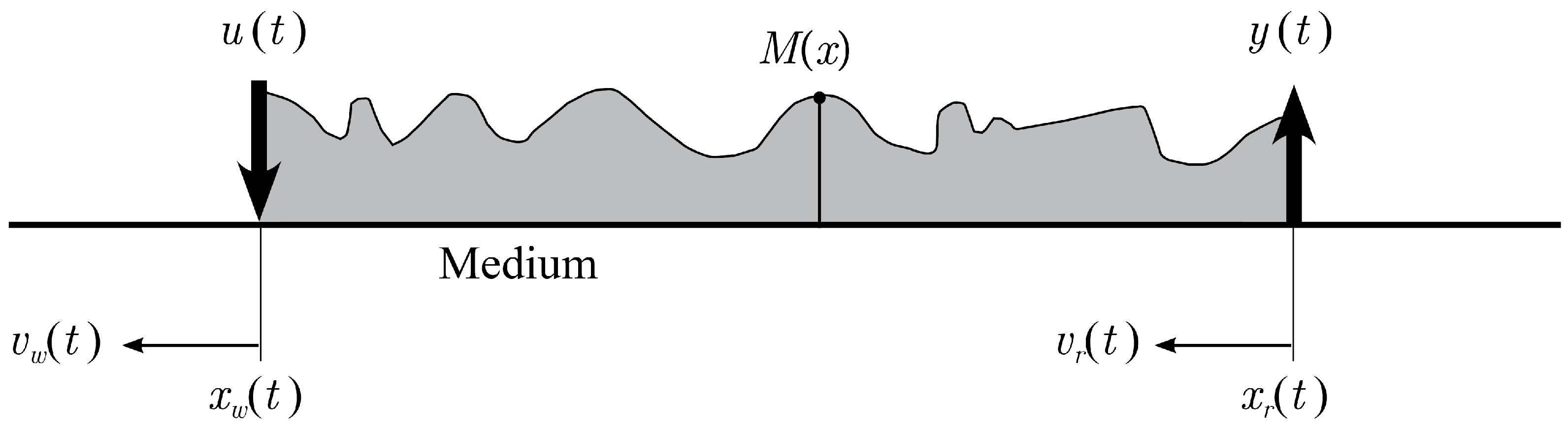
We now intend to develop a physically consistent model of the transfer delay. To do so, let us consider the kinematic framework illustrated in Figure 4, which depicts moving write and read heads relative to a transport medium with speeds $v_w\left(t\right)$ and $v_r\left(t\right)$, respectively. It is important to note that the model assumes that the reference frame is related to a medium whose velocity (in this frame) is zero. The positions of the write and read heads are denoted by $x_w\left(t\right)$ and $x_r\left(t\right)$ [m], respectively.

Figure 4. Kinematic representation of the transport delay model with moving write and read heads. The write head (input point) and read head (output point) move along the transport medium with speeds $v_w\left(t\right)$ and $v_r\left(t\right)$, respectively.

The terminology of write and read heads—borrowed from information storage systems and adopted in delay modeling [40]—provides a convenient abstraction for the physical input and output interfaces of the transport process.

The input signal of the delay model is $u\left(t\right)$ and the output (delayed) signal is $y\left(t\right)$. We assume that both quantities are scalar and dimensionally consistent (expressed in the same units).

The input signal is stored along the medium as a distributed function $M\left(x\right)$, where x takes values from the interval of length $L\left(t\right)$, which is the distance from the input head to the output head at time t:

$$L\left(t\right)=x_w\left(t\right)-x_r\left(t\right).$$

(8)

Since for transfer delay the power equals energy density times velocity, the boundary conditions are different for signal and transfer delays:

• Signal delay:

  $$M\left(x_w\left(t\right)\right)=u\left(t\right),M\left(x_r\left(t\right)\right)=y\left(t\right),$$

  (9)
• Transfer delay:

  $$M\left(x_w\left(t\right)\right)={\displaystyle \frac{u\left(t\right)}{v_w\left(t\right)}},M\left(x_r\left(t\right)\right)={\displaystyle \frac{y\left(t\right)}{v_r\left(t\right)}}.$$

  (10)

This ensures that for energy transfer its distribution along the medium $M\left(x\right)$ is expressed in J/m when input and output signals $u\left(t\right)$ and $y\left(t\right)$ are expressed in $\mathrm{W}=\mathrm{J}/\mathrm{s}$ and for mass transfer its distribution along the medium $M\left(x\right)$ is expressed in kg/m when input and output signals $u\left(t\right)$ and $y\left(t\right)$ are expressed in kg/s.

The positions of these heads evolve as:

$$x_w\left(t\right)={\int }_0^t{v}_w\left(\eta \right)d\eta +x_w\left(0\right),x_r\left(t\right)={\int }_0^t{v}_r\left(\eta \right)d\eta +x_r\left(0\right),$$

(11)

where $\eta$ is the integration variable [s], and $x_w\left(0\right)$ and $x_r\left(0\right)$ are the initial positions of the write and read heads [m], respectively. The transport distance $L\left(t\right)$ is measured in [m]. The delay $\tau \left(t\right)$ satisfies the kinematic condition:

$$x_r\left(t\right)=x_w(t-\tau \left(t\right)).$$

(12)

According to (11), Equation (12) becomes:

$${\int }_0^t{v}_r\left(\eta \right)d\eta +x_r\left(0\right)={\int }_0^{t-\tau \left(t\right)}{v}_w\left(\eta \right)d\eta +x_w\left(0\right).$$

(13)

Differentiating both sides with respect to time and applying the chain rule yields:

$$v_r\left(t\right)=v_w(t-\tau \left(t\right))\left(1-{\displaystyle \frac{d\tau \left(t\right)}{dt}}\right),$$

(14)

which after rearrangement gives the ODE describing changes in $\tau \left(t\right)$ caused by velocities $v_w\left(t\right)$ and $v_r\left(t\right)$:

$${\displaystyle \frac{d\tau \left(t\right)}{dt}}=1-{\displaystyle \frac{v_r\left(t\right)}{v_w(t-\tau \left(t\right))}}.$$

(15)

In variable-flow systems, neglecting the dependence of delay on velocity:

$$\tau \left(t\right)={\displaystyle \frac{L}{v\left(t\right)}},$$

(16)

violates energy conservation, leading to potential inaccuracies in thermal load prediction, erroneous storage sizing, or suboptimal control.

Combining the kinematic condition (12) with the boundary relations (10), and defining the dimensionless dynamic gain $k\left(t\right)={\displaystyle \frac{v_r\left(t\right)}{v_w(t-\tau \left(t\right))}}$, yields the coupled Transfer-Delay formulation:

$$\left\{\begin{array}{c}y\left(t\right)=k\left(t\right)u(t-\tau (t\left)\right)\hfill \\ {\displaystyle \frac{d\tau \left(t\right)}{dt}}=1-k\left(t\right)\hfill \\ k\left(t\right)={\displaystyle \frac{v_r\left(t\right)}{v_w(t-\tau \left(t\right))}}\hfill \end{array}\right.,$$

(17)

which ensures both kinematic and conservation consistency.

We assume positive velocities $v_w\left(t\right)>0$ and $v_r\left(t\right)>0$. This assumption implies $k\left(t\right)>0$, which leads to the bound:

$$-\infty <{\displaystyle \frac{d\tau \left(t\right)}{dt}}<1.$$

(18)

Note that $d\tau \left(t\right)/dt$ has no finite lower bound, as the ratio $v_r\left(t\right)/v_w(t-\tau \left(t\right))$ can grow arbitrarily large when extraction velocity significantly exceeds supply velocity.

The well-posedness (existence and uniqueness of solutions) of the system (15) is ensured by standard DDE theory [19] when $v_r\left(t\right)$ and $v_w\left(t\right)$ are continuous, bounded, and Lipschitz continuous—conditions inherently satisfied in physical systems with regulated actuators. The bound (18) guarantees causality and numerical stability, enabling reliable integration using standard DDE solvers.

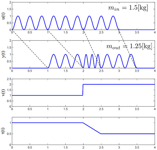
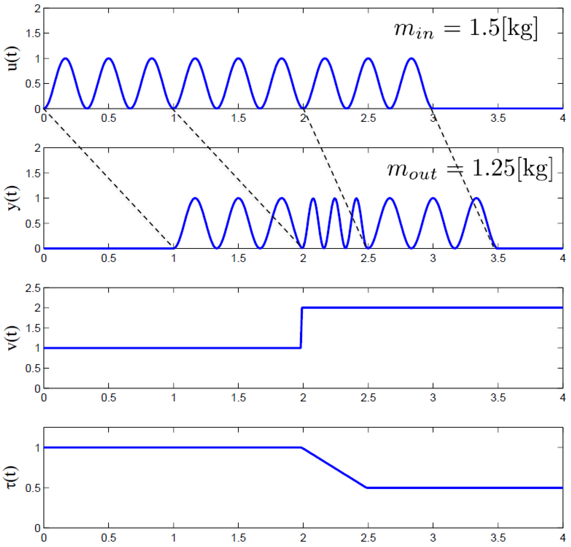
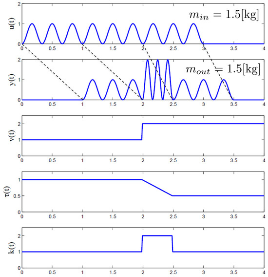
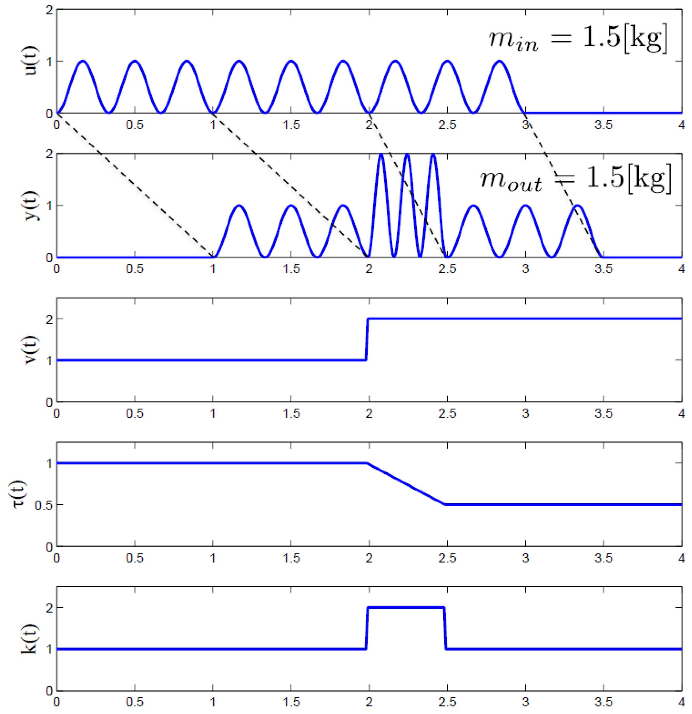
To validate this formulation, a third simulation was performed using the same setup as in Section 2.1.1 and Section 2.1.2. The proposed transfer-delay model (17) was implemented with explicit computation of the dynamic gain $k\left(t\right)$. The results are shown in Figure 5. Unlike the previous models, the output signal $y\left(t\right)$ exhibits neither amplitude loss nor spurious amplification. The dynamic gain $k\left(t\right)$, plotted in the bottom panel of Figure 5, adjusts continuously during the velocity transition to compensate for the redistribution of energy density along the transport medium. Quantitative integration confirms perfect mass conservation: the total input mass ($m_{in}=1.5$ kg) exactly equals the total output mass ($m_{out}=1.5$ kg), validating the physical consistency of the proposed formulation.

Figure 5. Simulation results for the proposed transfer-delay model (17). The absence of signal loss confirms conservation under variable flow conditions.

The resulting formulation provides a minimal physically consistent delay model suitable for dynamic energy systems with variable transport velocity.

2.3. Physical Interpretation of the Dynamic Gain $k\left(t\right)$

Because the dynamic coefficient $k\left(t\right)$ is important in distinguishing the Signal Delay from Transfer Delay models, it is worth giving it a physical interpretation to better understand its essence. Looking at its form:

$$k\left(t\right)={\displaystyle \frac{v_r\left(t\right)}{v_w(t-\tau \left(t\right))}},$$

(19)

we can see that it is the ratio of the speed at which the output signal is currently being read from the medium (at time t) to the speed at which the same signal was previously deposited in the medium (i.e., at time $t-\tau \left(t\right)$). This coefficient is dimensionless.

If we look at Figure 5 with the gain $k\left(t\right)$ graph, we can see that in the time interval from 2 [s] to 2.5 [s], it reaches a higher value of 2 because the current reading speed is 2 [m/s], but the same signal was previously recorded at a lower speed of 1 [m/s].

2.4. Assumptions and Limitations

The proposed transfer-delay framework is developed under several key assumptions that define its scope of applicability. The model assumes unidirectional transport with positive velocities $v_r\left(t\right)>0$ and $v_w\left(t\right)>0$, representing transport in a single direction without backflow. This is appropriate for systems with controlled pumps, valves, or natural flow direction, such as district heating supply lines and pipeline transport systems. The formulation further assumes incompressible flow with constant fluid density $\rho$ and specific heat c, which is valid for liquid transport (water, oils) over moderate temperature and pressure ranges covering most thermal energy systems. Transport is treated as a one-dimensional process along the pipeline length L with uniform cross-sectional properties, neglecting radial gradients, turbulence effects, and three-dimensional flow patterns. Additionally, input and output velocities $v_r\left(t\right)$ and $v_w\left(t\right)$ are assumed continuous and bounded, ensuring well-posedness of the delay differential Equation (15). This condition is satisfied in physical systems with actuator dynamics characterized by finite bandwidth and slew-rate limits.

The framework focuses on transport delay and conservation principles while neglecting distributed losses such as heat transfer to the environment, friction, or chemical reactions along the transport path. Such effects can be superimposed as additional terms if needed but are not included in the core formulation. The model does not currently support compressible flows where gas transport involves significant density variations, such as in high-pressure hydrogen pipelines; extension to such systems would require incorporating wave propagation and pressure-volume work. Similarly, bidirectional flows or recirculating systems, such as thermal storage with reversible charging and discharging through the same path, would require modifications to handle velocity sign changes and their implications for delay dynamics. Systems where radial temperature gradients, mixing, or dispersion significantly affect transport dynamics may require partial differential equation (PDE) models rather than the lumped delay approach presented here.

While the framework is validated against representative simulation scenarios in Section 5, experimental validation with industrial-scale systems remains a direction for future work. These assumptions and limitations define the boundaries within which the proposed framework provides physically consistent results and guide appropriate application to practical systems. Its broader implications and classification are discussed in Section 3.

3. Classification of Variable Delays

Building upon the preceding mathematical formulation, this section introduces a systematic classification of variable delays according to their type and kind. The proposed taxonomy distinguishes between informational and physical transport processes and identifies which transport element introduces time variability. This structured approach addresses a major limitation of prior studies, in which delay representations were often applied uniformly without accounting for their physical origin or conservation laws.

The type refers to the nature of the transported quantity. A signal delay represents the transmission of information, where the amplitude is preserved and conservation laws are not relevant. It is mathematically expressed as $y\left(t\right)=u(t-\tau (t\left)\right)$, typical for communication or sensor networks. In contrast, a transfer delay refers to the physical transport of mass or energy, where the amplitude depends on the time-varying gain $k\left(t\right)$ and conservation principles must hold, as described by (15). Such delays are characteristic of industrial processes involving energy or material transport, such as pipelines, conveyor systems, and thermal networks.

The kind of delay specifies which velocity component introduces the delay time variability:

1.

Type R—variable read-head velocity $v_r\left(t\right)$, representing changes in the place where the delayed signal is read (e.g., the place where the material is collected from the conveyor belt);

2.

Type W—variable write-head velocity $v_w\left(t\right)$, representing changes in the place where the input signal is transmitted to the delay element (e.g., the place where the material is deposited on the conveyor belt);

3.

Type M—variable speed of the medium relative to both stationary heads, corresponding to the situation when the positions of both heads change simultaneously in the same way relative to the stationary medium at speed $v\left(t\right)=v_w\left(t\right)=v_r\left(t\right)$ (e.g., the speed of a conveyor belt or the speed of a pump in a pipeline).

Table 1 summarizes the corresponding expressions for the gain $k\left(t\right)$ and delay evolution $\dot{\tau }\left(t\right)$ derived from the general transfer delay model (15) and the delay dynamics (8). This overview shows how variability in specific transport elements—write-head, read-head, or medium—affects overall delay behavior and system dynamics. The modular structure of this formulation facilitates its adaptation to a wide range of energy and industrial applications.

Table 1. Mathematical models for different kinds of variable delays.

Type of Delay	Variable(s) Controlling the Time Delay		Signal Delay	Transfer Delay
	Constant	Variable	$\mathit{y}\left(\mathit{t}\right)=\mathit{u}(\mathit{t}-\mathit{\tau }(\mathit{t}\left)\right)$	$\mathit{y}\left(\mathit{t}\right)=\mathit{k}\left(\mathit{t}\right)·\mathit{u}(\mathit{t}-\mathit{\tau }(\mathit{t}\left)\right)$
	Speed(s)	Speed(s)	${\displaystyle \frac{\mathit{d}\mathit{\tau }\left(\mathit{t}\right)}{\mathit{dt}}}=\mathit{1}-\mathit{k}\left(\mathit{t}\right)$	${\displaystyle \frac{\mathit{d}\mathit{\tau }\left(\mathit{t}\right)}{\mathit{dt}}}=\mathit{1}-\mathit{k}\left(\mathit{t}\right)$
General	–	$v_w\left(t\right)$ and $v_r\left(t\right)$	$k\left(t\right)={\displaystyle \frac{v_r\left(t\right)}{v_w(t-\tau \left(t\right))}}$
Type R	$v_w=\mathrm{const}$	$v_r\left(t\right)$	$k\left(t\right)={\displaystyle \frac{v_r\left(t\right)}{v_w}}$
Type W	$v_r=\mathrm{const}$	$v_w\left(t\right)$	$k\left(t\right)={\displaystyle \frac{v_r}{v_w(t-\tau \left(t\right))}}$
Type M	–	$v_w\left(t\right)=v_r\left(t\right)=v\left(t\right)$	$k\left(t\right)={\displaystyle \frac{v\left(t\right)}{v(t-\tau (t\left)\right)}}$

Representative Applications

The proposed classification enables consistent identification of delay mechanisms in both energy systems and other engineering domains. In district heating networks, one can use Transfer Delay of Type R, where the variable read-head velocity $v_r\left(t\right)$ determines the effective delay [24,25,41]. Conversely, in renewable power generation one can use Transfer Delay of Type W [31,32]. In the field of thermal energy storage using phase-change materials exemplifies usually a Type M delay [26]. Finally, signal delays occur in communication-based control, such as PMU-based monitoring in smart grids, where time-varying latency affects only data reception [28,42].

Beyond energy systems, the same taxonomy applies to chemical and biological processes: variable feed or extraction in reactors (Types W and R) [43], variable conveyor speeds in mechanical systems (Type M), or physiological transport mechanisms such as blood flow or gas exchange [17,44,45], combustion dynamics in engines [46], and circulating fluidized bed boilers [47]. This generality demonstrates the broad applicability of the framework across physical and cyber–physical domains.

Correct identification of delay type and kind is essential for constructing accurate and physically consistent simulation models. Inappropriate simplifications—such as representing a transfer delay as a signal delay—can lead to significant errors in performance prediction, particularly in energy networks with variable supply and demand. The proposed classification therefore provides both a theoretical foundation and a practical guideline for developing simulation models that preserve conservation principles and causal consistency.

4. Implementation in Simulink Environment

Implementing the proposed delay models in the Simulink environment required developing new functional blocks, since the standard library does not support all types of time-varying delays. Simulink natively provides two blocks capable of simulating variable delays: the Variable Time Delay block, which corresponds to the R-type Signal Delay, and the Variable Transport Delay block, which corresponds to the M-type Signal Delay. As demonstrated in Section 2, the Variable Transport Delay cannot be directly applied in mass and energy transport simulations. This limitation highlights the need to extend the Simulink library with blocks capable of representing both Signal Delay and Transfer Delay, in all three variants (Table 2).

Table 2. Delay blocks available in Simulink and those newly developed, classified by type and kind.

Variable(s) Controlling the Time Delay	Type of Delay
	Signal Delay	Transfer Delay
$v_w\left(t\right)=v_r\left(t\right)=v\left(t\right)$	Signal Delay M (Simulink: Variable Transport Delay)	Transfer Delay M (Newly developed)
$v_r\left(t\right)$ ($v_w=\mathrm{const}$)	Signal Delay R (Simulink: Variable Time Delay)	Transfer Delay R (Newly developed)
$v_w\left(t\right)$ ($v_r=\mathrm{const}$)	Signal Delay W (Newly developed)	Transfer Delay W (Newly developed)

4.1. General Delay Blocks

Two general-purpose blocks, named Signal Delay and Transfer Delay, were implemented based on the mathematical models presented in Table 1. Their inputs are the delayed signal $u\left(t\right)$ and the instantaneous values of the read and write speeds, $v_r\left(t\right)$ and $v_w\left(t\right)$. The output is computed according to the following equations:

$$y\left(t\right)=u(t-\tau \left(t\right)),{\displaystyle \frac{d\tau \left(t\right)}{dt}}=1-{\displaystyle \frac{v_r\left(t\right)}{v_w(t-\tau \left(t\right))}},$$

(20)

for the Signal Delay block, and

$$y\left(t\right)={\displaystyle \frac{v_r\left(t\right)}{v_w(t-\tau \left(t\right))}}u(t-\tau \left(t\right)),{\displaystyle \frac{d\tau \left(t\right)}{dt}}=1-{\displaystyle \frac{v_r\left(t\right)}{v_w(t-\tau \left(t\right))}},$$

(21)

for the Transfer Delay block.

These formulations ensure consistency with the general case introduced in the mathematical framework.

4.2. Delay Blocks with Time Parameter

On the basis of the general-purpose blocks, parameterized delay blocks were developed. In these blocks, the user specifies a nominal delay ${\tau }_i\left(t\right)$, which is internally transformed into the equivalent read and write head velocities according to the selected variant (R, W, or M). These velocities are then used as inputs to the corresponding Signal Delay or Transfer Delay block.

The functional equations implemented in the blocks are consistent with the definitions introduced in Section 3, i.e.,

$$y\left(t\right)=u(t-\tau (t\left)\right)(\mathrm{Signal}\mathrm{Delay}),$$

(22)

$$y\left(t\right)={\displaystyle \frac{v_r\left(t\right)}{v_w(t-\tau \left(t\right))}}u(t-\tau \left(t\right))(\mathrm{Transfer}\mathrm{Delay}).$$

(23)

Depending on the choice of variant (R, W, or M), the internal delay $\tau \left(t\right)$ is determined using the relationships derived previously. This modular construction enables the simulation of all six types of delays defined in the classification.

To improve robustness, additional protection mechanisms were implemented. Negative values of ${\tau }_i\left(t\right)$ are automatically saturated to zero, and a warning is issued to the user through an integrated validation block.

The developed transfer-delay blocks were subsequently embedded in the heat transport in pipeline systems (case study Section 5) to validate the proposed formulation under realistic operating scenarios.

5. Case Study: Heat Transport in Pipeline System

This section demonstrates the practical application of the proposed transfer-delay formulation to a representative energy system and reveals the consequences of using physically inconsistent delay models. The selected example concerns heat transport in a pipeline with variable pump control, which is fundamental to modern energy engineering and industrial process control.

5.1. Physical Context and System Description

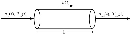
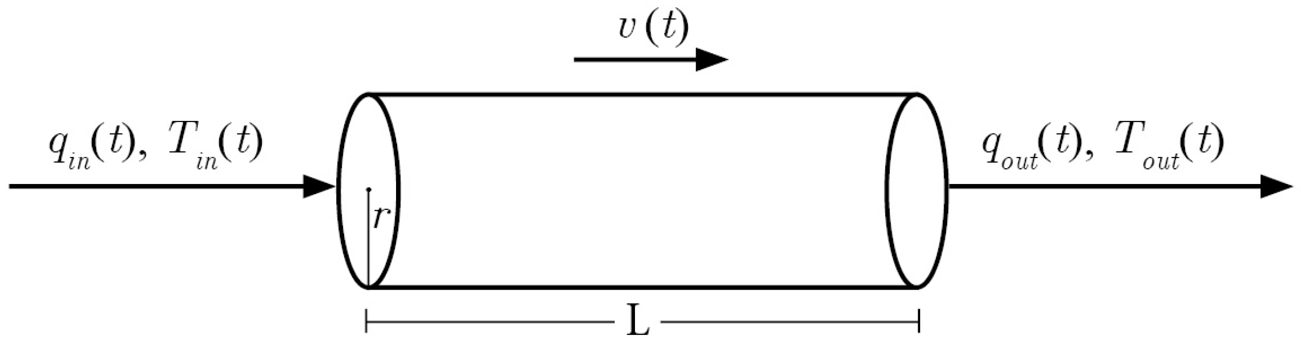
Consider a district heating pipeline of fixed length L, connecting a heat source to a consumer (Figure 6). The system operates under variable-flow control, where the pump speed—and consequently the fluid velocity $v\left(t\right)$—is dynamically adjusted to match thermal demand or optimize energy efficiency. Such modulation of flow is common in district heating networks [27], industrial heat recovery systems, and thermal management loops in power plants.

Figure 6. Schematic representation of the heating pipeline under analysis.

The system is characterized by:

• Input thermal energy flow $q_{in}\left(t\right)$ [J/s = W] entering the pipeline;
• Input temperature $T_{in}\left(t\right)$ [°C];
• Output thermal energy flow $q_{out}\left(t\right)$ [J/s = W] delivered to the consumer;
• Output temperature $T_{out}\left(t\right)$ [°C];
• Medium velocity $v\left(t\right)$ [m/s], controlled by pump speed;
• Pipeline length L 3600 [m] (constant);
• Pipeline radius r = 0.1 [m];
• Specific heat of water $c=4.184\mathrm{kJ}$/[kg°C].

Assuming constant fluid density and specific heat, the principle of energy conservation becomes equivalent to that of mass conservation. The thermal energy flow $q\left(t\right)$ is proportional to the mass flow rate $\dot{m}\left(t\right)$, which depends on $v\left(t\right)$ and the pipe cross-sectional area.

5.2. Application of Transfer Delay Framework

Both the inlet and outlet positions are fixed, while the medium velocity $v\left(t\right)$ is varied via pump control. This represents a Type M (Medium-variable) Transfer Delay, where $v_w\left(t\right)=v_r\left(t\right)=v_m\left(t\right)=v\left(t\right)$. The variable velocity directly affects both transport delay and energy density distribution along the pipeline.

The governing equations, specialized for Type M, are

$$\left\{\begin{array}{c}{q}_{out}\left(t\right)=k\left(t\right)·q_{in}(t-\tau \left(t\right)),\hfill \\ {\displaystyle \frac{d\tau \left(t\right)}{dt}}=1-k\left(t\right),\hfill \\ k\left(t\right)={\displaystyle \frac{v\left(t\right)}{v(t-\tau (t\left)\right)}},\hfill \end{array}\right.$$

(24)

where the dimensionless gain $k\left(t\right)$ ensures energy conservation under variable-flow conditions by compensating for redistribution of the linear energy density $\left[\mathrm{J}/\mathrm{m}\right]$ when $v\left(t\right)$ changes. The delay $\tau \left(t\right)$ represents the propagation time of thermal perturbations: as $v\left(t\right)$ increases, $\tau \left(t\right)$ decreases and vice versa.

To facilitate comparison, the formulation was implemented in Simulink using a custom block that updates both $\tau \left(t\right)$ and $k\left(t\right)$ at each integration step, ensuring dynamic consistency between delay and gain evolution.

5.3. Comparative Simulation Setup

To highlight the implications of the formulation, three previously defined models were compared under identical conditions:

• Model 1—a pure signal-based Variable Time Delay;
• Model 2—Simulink’s Variable Transport Delay block (no dynamic scaling);
• Model 3—the proposed Transfer Delay (Type M) including dynamic gain $k\left(t\right)$.

The distinction between Models 2 and 3 is subtle but important: Model 2 uses Simulink’s dedicated transport delay block, which internally manages the delay buffer and attempts to represent material transport, whereas Model 3 treats the delay as a generic time shift without any physical interpretation. Both, however, fail to enforce conservation laws.

A thermal power pulse $q_{in}\left(t\right)$ was introduced at the inlet, while $v\left(t\right)$ was varied to emulate realistic pump control. The comparison focuses on total input and output energies to verify conservation. The comparison focuses on both qualitative signal behavior and quantitative energy balance, allowing verification of the conservation principle under dynamic velocity conditions.

5.4. Simulation Results

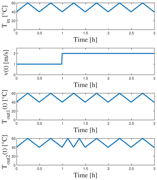
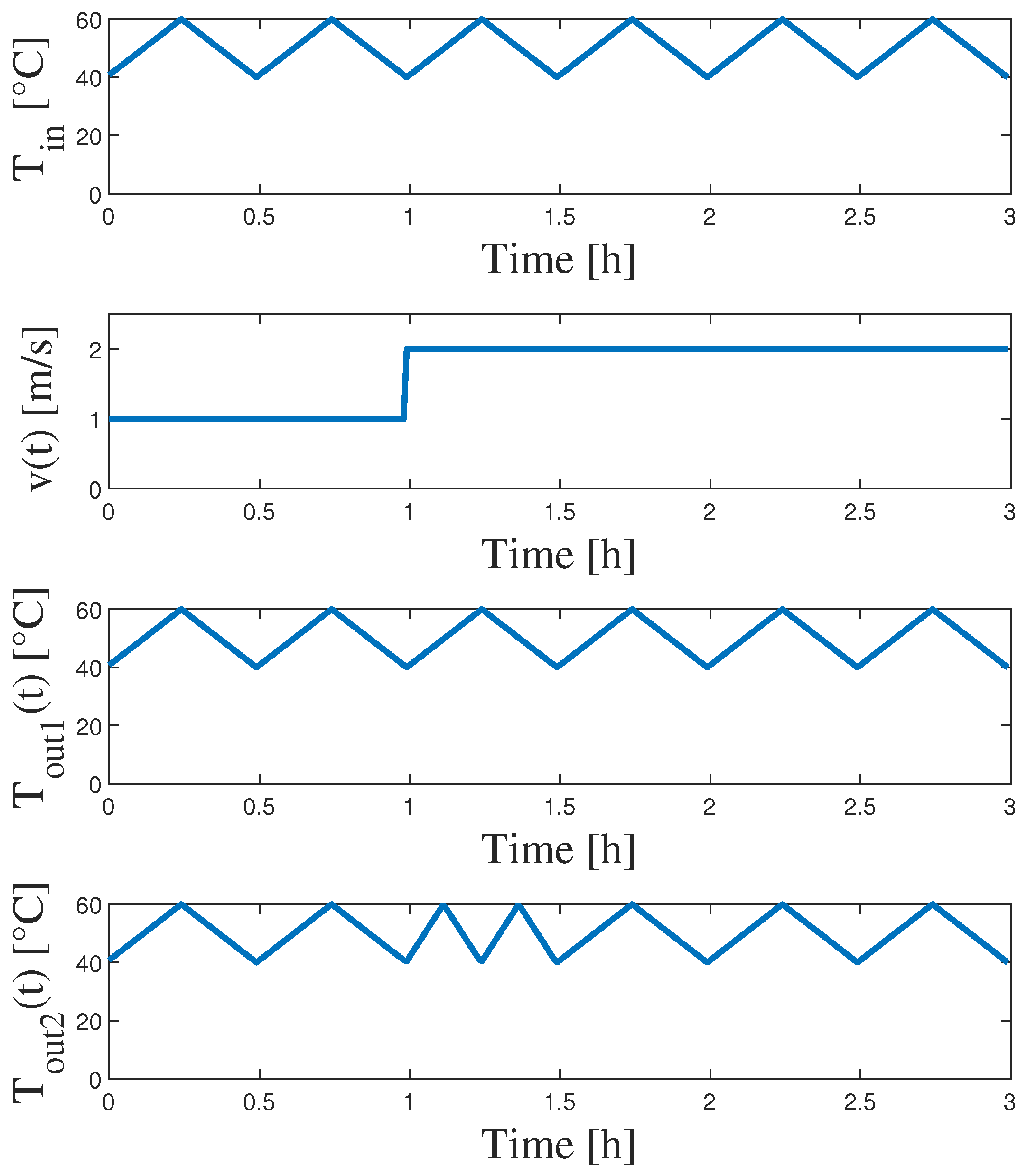
The simulation aims to validate the physical consistency of the proposed transfer-delay formulation and to quantify deviations introduced by conventional delay implementations. Figure 7 presents a comprehensive comparison of different delay models under variable-flow conditions for input and output temperatures of the pipeline.

Figure 7. Input temperature course in a given system (top) and results of the output temperature courses for different analyzed models (Model 1— $T_{out1}$, Model 2—$T_{out2}$) of delay time change caused by increased water speed $v\left(t\right)$ in the analyzed pipeline system.

5.4.1. Temperature Simulation

Figure 7 shows the simulation results for the temperature evolution through the pipeline. The top panel displays the input temperature $T_{in}\left(t\right)$ as a triangular wave oscillating between 40 °C and 60 °C with a period of approximately 0.5 h, representing the diurnal changes in the heat source temperature caused, for example, by relay (bang-bang) control of the source temperature. The second panel shows the medium velocity $v\left(t\right)$, which undergoes a step change from 1 m/s to 2 m/s at $t=1$ h, simulating an increase in pump speed to accommodate higher thermal demand.

The two subsequent panels reveal the output temperature responses for different modeling approaches:

• Model 1 ($T_{out1}\left(t\right)$, fourth panel) uses a pure signal-based Variable Time Delay. This model also shows qualitatively correct temporal shifting of the temperature profile, with similar compression of oscillations following the velocity increase. The output closely matches Model 1, demonstrating that for temperature propagation, the signal-delay approach yields acceptable results.
• Model 2 ($T_{out2}\left(t\right)$, third panel) employs Simulink’s Variable Transport Delay block. The output faithfully reproduces the triangular input waveform with correct temporal shifting. After the velocity step at $t=1$ h, the delay $\tau \left(t\right)=L/v\left(t\right)$ decreases from 1 h to 0.5 h, causing the output oscillations to compress temporally while maintaining their amplitude. The temperature profile remains undistorted, with peak and trough values matching the input.

This behavior is physically consistent with the nature of temperature as an intensive (non-extensive) quantity. Temperature represents a local thermodynamic state and does not obey additive conservation laws like mass or energy. Its propagation through the pipeline is governed purely by advection (bulk fluid motion) without requiring redistribution or scaling. Mathematically, temperature transport follows

$$T_{out}\left(t\right)=T_{in}(t-\tau \left(t\right)),$$

(25)

which is precisely the signal-delay formulation. Consequently, both Model 1 and Model 2—conventional Simulink delay blocks without dynamic gain—are suitable for accurately simulating temperature evolution under variable flow conditions. The delay time $\tau \left(t\right)$ adjustment caused by the velocity step is correctly captured by both models, as evidenced by the synchronized compression of output waveforms after $t=1$ h.

This result underscores an important distinction: while standard delay implementations are adequate for intensive quantities like temperature or concentration, they fundamentally fail for extensive quantities (mass, energy, momentum) that require conservation-consistent modeling with the dynamic gain $k\left(t\right)$, as demonstrated in the subsequent thermal power analysis.

5.4.2. Thermal Energy Flow Simulation

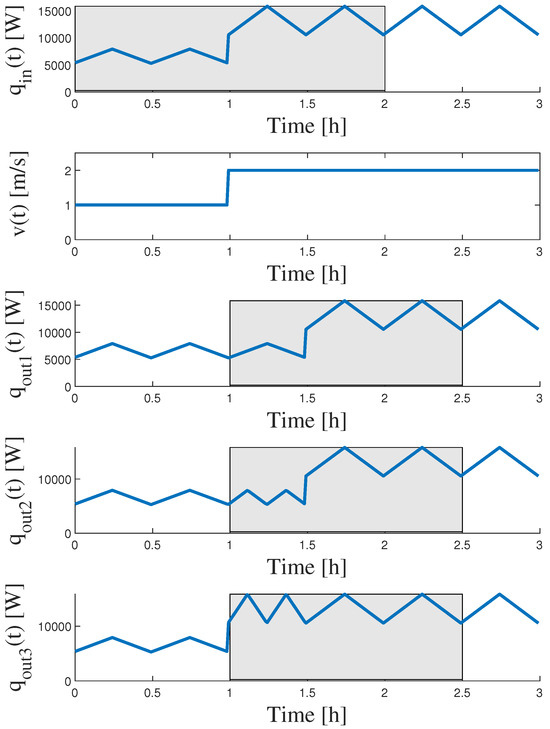
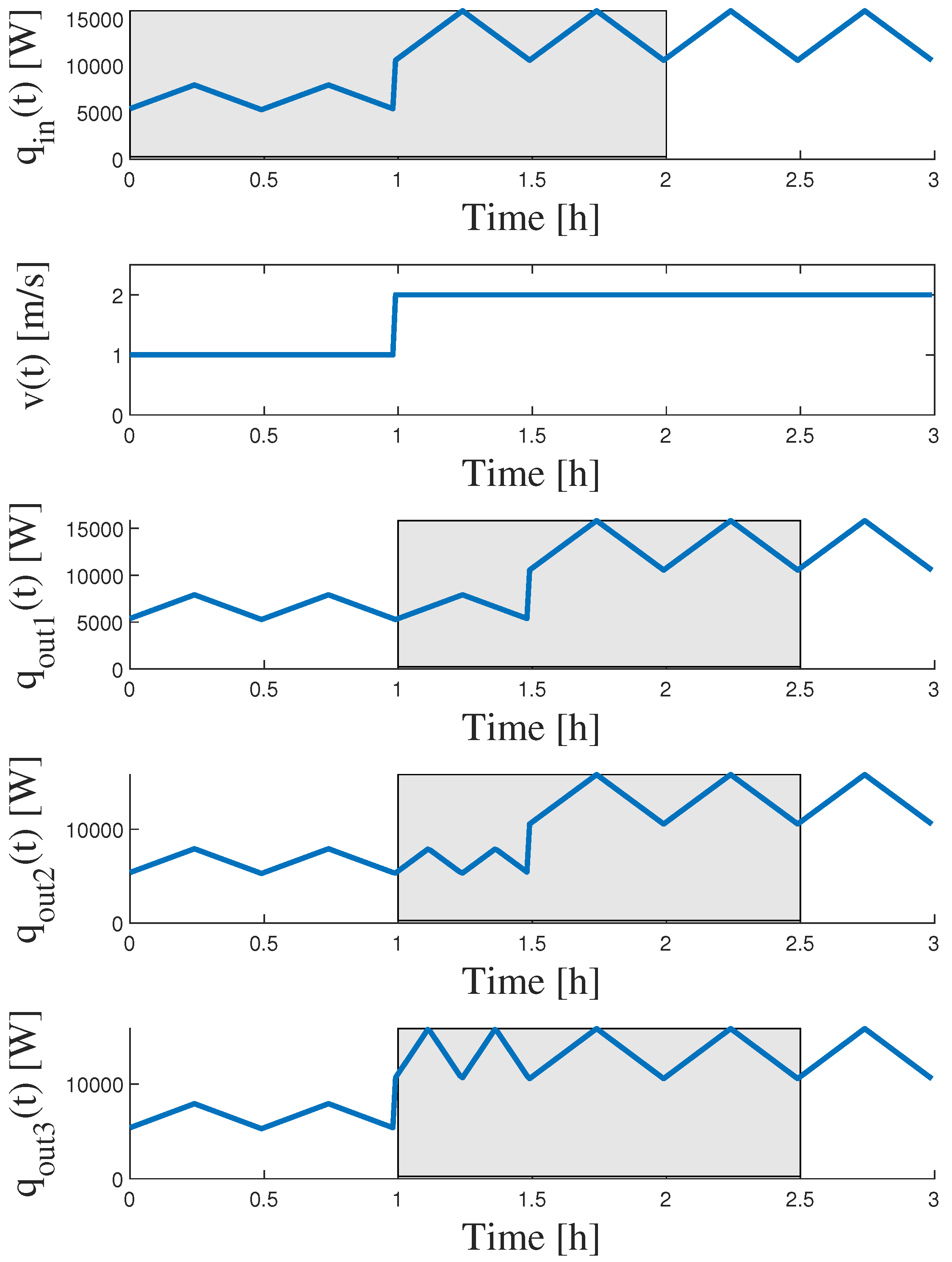
Figure 8 shows the simulation results for the thermal energy flow under the same simulation conditions as in a previous subsection. The upper panel displays the input thermal power $q_{in}\left(t\right)$ as an oscillating wave with variable amplitude (ranging from approximately 5000 W to 15,000 W), corresponding to temperature changes presented in a previous subsection. The second panel displays the medium velocity $v\left(t\right)$, which undergoes a step change from 1 m/s to 2 m/s at $t=1$ h.

Figure 8. Simulation results comparing Model 1 ($q_{out1}$), Model 2 ($q_{out2}$), Model 3 ($q_{out3}$). Gray boxes represent the analyzed time intervals for comparison of the total thermal energy transferred through the pipeline system (see Table 3).

To facilitate quantitative comparison, the time interval $t\in [1,2.5]$ h (indicated by gray shading in Figure 8) is selected for detailed energy balance analysis. This window follows directly from the system’s kinematic properties: with an initial transport delay of $\tau =L/v=3600/1=1$ h, decreasing to $\tau =L/v=3600/2=0.5$ h after the velocity step, the input interval $t\in [0,2]$ h maps precisely to the output interval $t\in [1,2.5]$ h. The selected window therefore corresponds to the complete transported signal at the output, ensuring a physically meaningful and fair energy balance comparison across all three models.

The subsequent three panels (Figure 8) reveal striking differences in model behavior for the thermal energy flow $q\left(t\right)$, which is an extensive quantity and must conserve energy:

• Model 1 ($q_{out1}\left(t\right)$, third panel), the Simulink Signal Delay block, and Model 2 ($q_{out2}\left(t\right)$, fourth panel), the Simulink Variable Transport Delay block, both show significant amplitude reduction and phase-shifted oscillations immediately following the velocity transition at $t=1$ h. While the waveform shape is qualitatively preserved, the output amplitude is systematically lower than the input, indicating progressive energy loss. These conventional models enforce kinematic delay evolution but omit the conservation-mandating dynamic gain term $k\left(t\right)$, resulting in non-physical energy dissipation, as confirmed by the quantitative analysis.
• Model 3 ($q_{out3}\left(t\right)$, fifth panel), which is the proposed Transfer Delay (Type M) including the dynamic gain $k\left(t\right)$, faithfully preserves energy conservation through correct amplitude scaling. Notably, after the velocity step at $t=1$ h, the output amplitude in the gray-shaded region exceeds the input amplitude due to the compensating action of the dynamic gain $k\left(t\right)=v\left(t\right)/v(t-\tau (t\left)\right)$. When velocity doubles, the linear energy density [J/m] along the pipe is compressed, and this compression is correctly reflected in the output power through the gain factor $k\left(t\right)\approx 2$, ensuring that total energy is conserved despite the kinematic compression of the thermal wave.

A visual comparison within the gray-shaded analysis interval clearly indicates that only Model 3 preserves the essential characteristics and magnitude necessary for correct energy balance under dynamic flow conditions.

5.4.3. Quantitative Analysis of Energy Conservation

Table 3 summarizes the total energy balance results for the thermal energy flow $q\left(t\right)$, confirming the quantitative differences between the models based on integration over the analysis interval $t\in [1,2.5]$ h.

Table 3. Comparison of total output thermal energy for different models over the analysis interval $t\in [1,2.5]$ h (gray-shaded region in Figure 8). Total input energy ${\int }_1^{2.5}{q}_{in}\left(t\right)dt=100$ J is constant across all simulations.

Model	Total Input Energy [J]	Total Output Energy [J]
1	100	74.8
2	100	74.8
3	100	99.8

The results confirm that only Model 3, the proposed transfer-delay model including the dynamic gain $k\left(t\right)$, achieves near-perfect conservation of energy, with output energy (99.8 J) almost exactly matching the input energy (100 J). The small 0.2 J discrepancy (0.2%) is attributable to numerical integration errors and finite simulation timestep, confirming the physical consistency of the proposed formulation for extensive quantities.

In contrast, both Model 1 (Simulink Signal Delay) and Model 2 (Simulink Variable Transport Delay) exhibit a significant energy loss of 25.2 J (100 J input vs. 74.8 J output), representing an energy dissipation of approximately 25% over the analysis interval. This unphysical dissipation demonstrates that standard delay implementations, regardless of whether they are transport-based or pure signal shifts, violate conservation laws when applied to variable-velocity transport systems for thermal energy flow $q\left(t\right)$.

5.4.4. Overall Conclusion

The observed energy imbalance in Models 1 and 2 has significant practical implications for district heating network design and operation. In real systems, a 25% underestimation of delivered thermal energy would lead to severe consequences: undersizing of heat exchangers, incorrect prediction of consumer comfort levels, and erroneous assessment of system capacity during peak demand periods. In renewable energy integration studies involving thermal storage with variable charging/discharging rates, conservation violations of this magnitude would fundamentally compromise the reliability of techno-economic analyses and control strategy development.

These results underscore the necessity of employing physically consistent delay models that explicitly couple kinematic evolution with conservation principles through the dynamic gain term $k\left(t\right)$ when simulating extensive quantities (such as thermal energy flow $q\left(t\right)$, mass flow rate, or momentum) under variable-flow conditions. Conversely, for non-extensive (intensive) quantities such as temperature $T\left(t\right)$ or concentration the Simulink Variable Transport Delay (Model 2) provides sufficiently accurate results, as demonstrated in Section 5.4.1.

The case study validates that only the proposed transfer-delay model (Model 3) preserves energy consistency under dynamically varying flow, confirming its suitability and necessity for realistic thermal power system simulations in district heating networks, industrial heat recovery systems, and other energy transport applications involving variable flow control.

6. Conclusions

Computer simulation is a fundamental tool in the analysis of dynamical systems with delays. However, it has been demonstrated that relying solely on standard simulation blocks without accounting for underlying physical principles can lead to unphysical results and severe inaccuracies. This challenge is particularly critical in energy systems, where inaccurate delay modeling violates conservation laws, potentially compromising economic efficiency and grid stability.

6.1. Key Contributions and Physical Significance

A rigorous framework for modeling time-varying delays in physical transport systems has been provided, directly addressing the limitations of conventional signal-shift models:

• Physically consistent formulation: A unified mathematical framework (Equation (15)) for transfer delays was developed, explicitly coupling kinematic evolution with conservation laws. The introduction of the time-varying gain $k\left(t\right)$ ensures both dimensional consistency and the preservation of energy and mass balance, a capability fundamentally absent in standard Signal Delay models.
• Systematic classification framework: A dual classification scheme was introduced, distinguishing between Signal Delays (information transfer) and Transfer Delays (physical transport), further categorized by the source of variability (Types R, W, and M). This taxonomy provides a practical guideline for consistent model selection across diverse domains, including district heating, power-to-gas, and thermal storage.
• Implementation and validation: New functional blocks for the Simulink environment were developed, supporting all six delay variants, thereby extending the capability of industrial simulation tools. Validation through a heat transport case study confirmed that while standard models fail in conservation, the proposed transfer-delay formulation maintains physical consistency under variable operating conditions.

Correct identification and modeling are crucial for accurate thermal load prediction, optimal sizing of energy storage, and reliable control system design in complex energy systems.

6.2. Limitations of the Current Framework

The proposed mathematical framework, while broadly applicable, operates within specific boundaries that define its scope.

The formulation assumes incompressible flow with constant fluid properties—density $\rho$ and specific heat c. This assumption is well justified for liquid transport in thermal energy systems operating over moderate temperature and pressure ranges, such as district heating networks. However, it precludes direct application to gas transport systems, such as high-pressure hydrogen pipelines or natural gas networks, where density variations are significant and wave propagation effects cannot be neglected. Extending the framework to compressible flows would require incorporating pressure–volume work and acoustic dynamics, fundamentally changing the structure of the delay evolution Equation (15).

The model is developed for unidirectional transport with strictly positive velocities ($v_w(t-\tau \left(t\right))>0$), as expressed by constraint (18). This condition is physically motivated and automatically satisfied in systems with regulated actuators, such as pumps and valves with finite slew rates. However, it excludes bidirectional or recirculating systems—for example, thermal storage units where the same pipeline is used alternately for charging and discharging—which would require modifications to handle velocity sign changes and their implications for delay dynamics and conservation.

The framework treats transport as a one-dimensional process along the pipeline length L, with uniform cross-sectional properties. This is appropriate when radial gradients are negligible and flow is well-mixed, as in most forced-convection liquid systems. However, in systems where radial temperature gradients, dispersion, or multidimensional flow patterns play a significant role—such as large-diameter pipes, stratified storage tanks, or heat exchangers with complex geometry—the lumped delay approach may not capture the relevant dynamics, and distributed parameter (PDE-based) models would be more appropriate.

The formulation also focuses specifically on transport delay and conservation, and does not account for distributed losses along the transport path, such as heat transfer to the environment through pipe walls, viscous friction, or chemical reactions. In district heating networks, for instance, thermal losses along long pipelines can be significant and affect both the amplitude and shape of the delivered thermal power signal. While such effects can in principle be superimposed as additional terms on top of the delay model, their systematic integration with the conservation-consistent delay formulation is not addressed in this work.

Finally, the framework has been validated through simulation case studies representing realistic operating scenarios (Section 5). However, experimental validation with industrial-scale energy systems—district heating networks, power-to-gas installations, or thermal storage facilities—remains an important step to quantify modeling accuracy under real-world conditions. Field measurements introduce additional complexity through sensor noise, unmodeled disturbances, parameter uncertainty, and spatially distributed effects that are absent in simulation.

Quantifying the impact of these factors on the performance of the proposed transfer-delay formulation relative to conventional models is an important direction for future validation work. These limitations do not diminish the framework’s utility for the broad class of applications discussed in Section 3, but they define the boundaries within which the model provides physically consistent results.

6.3. Limitations and Directions for Future Research

The proposed mathematical framework for time-varying delays has broad applicability beyond energy systems. Similar conservation-consistent formulations are needed in biomedical engineering, where delay differential equations model physiological regulatory mechanisms [10,11], predict the impact of ionizing radiation on living organisms [12], simulate functional components of biological systems [13], describe drug delivery and pharmacokinetic dynamics [14], and analyze infectious disease progression and cancer growth [15]. In these applications, transport delays fundamentally affect therapeutic outcomes and predictive accuracy. The framework also extends to chemical process control [46], hydraulic networks [47], and cardiovascular dynamics [44], where conservation principles are equally critical. Mathematical modeling with delay differential equations enables both analysis and prediction of complex biological system behavior [45], making the generality of the classification scheme (Types R, W, M) valuable for technology transfer across these domains.

The current formulation assumes incompressible flow and requires strictly positive transport velocities ($v_w(t-\tau \left(t\right))>0$), as expressed by constraint (18). Future research directions are focused on extending the framework to compressible flow regimes and incorporating it into advanced control design methodologies:

• Development of stability criteria and robust controller design specifically tailored to systems governed by transfer delays.
• Integration into Model Predictive Control strategies for renewable energy systems to proactively compensate for variable delays.
• Experimental validation on industrial-scale thermal systems to quantify performance improvements.
• Generalization to multiphase and compressible flows and application to large-scale distributed energy networks.

The methodology presented in this work provides a rigorous foundation and practical tools for accurate and physically sound delay modeling, which is essential for meeting the challenges of the evolving energy transition.

References

- Niculescu, S.-I. Delay Effects on Stability: A Robust Control Approach; Springer: Berlin/Heidelberg, Germany, 2001. [Google Scholar] [CrossRef] [Scilit]
- Sipahi, R.; Niculescu, S.-I.; Abdallah, C.T.; Michiels, W.; Gu, K. Stability and Stabilization of Systems with Time Delay. IEEE Control Syst. Mag. 2011, 31, 38–65. [Google Scholar] [CrossRef] [Scilit]
- Fujarewicz, K.; Łakomiec, K. Parameter estimation of systems with delays via structural sensitivity analysis. Discret. Contin. Dyn.-Syst. 2014, 19, 2521–2533. [Google Scholar] [CrossRef] [Scilit]
- Fujarewicz, K. Estimation of initial functions for systems with delays from discrete measurements. Math. Biosci. Eng. 2017, 14, 165–178. [Google Scholar] [CrossRef] [Scilit]
- European Commission. Fit for 55: Delivering the EU’s 2030 Climate Target on the Way to Climate Neutrality; European Commission: Brussels, Belgium, 2021; Available online: https://ec.europa.eu/info/strategy/priorities-2019-2024/european-green-deal/delivering-european-green-deal_en (accessed on 15 October 2025).
- Zhang, Y.; Pen, H.; Zhang, X. Stability Control of Grid-Connected Converter Considering Phase-Locked Loop Frequency Coupling Effect. Energies 2024, 17, 3438. [Google Scholar] [CrossRef] [Scilit]
- Ding, L.; Han, Q.-L.; Ge, X.; Zhang, X.-M. An Overview of Recent Advances in Event-Triggered Consensus of Multiagent Systems. IEEE Trans. Cybern. 2018, 48, 1110–1123. [Google Scholar] [CrossRef] [Scilit]
- Cagnano, A.; De Tuglie, E.; Mancarella, P. Microgrids: Overview and guidelines for practical implementations and operation. Appl. Energy 2020, 258, 114039. [Google Scholar] [CrossRef] [Scilit]
- Nosratabadi, S.M.; Hooshmand, R.-A.; Gholipour, E. A comprehensive review on microgrid and virtual power plant concepts employed for distributed energy resources scheduling in power systems. Renew. Sustain. Energy Rev. 2017, 67, 341–363. [Google Scholar] [CrossRef] [Scilit]
- Mackey, M.C.; Glass, L. Oscillation and chaos in physiological control systems. Science 1977, 197, 287–289. [Google Scholar] [CrossRef] [Scilit]
- Bélair, J.; Glass, L.; an der Heiden, U.; Milton, J. Dynamical disease: Identification, temporal aspects and treatment strategies of human illness. Chaos 1995, 5, 1–7. [Google Scholar] [CrossRef] [Scilit] [PubMed]
- Fenwick, J.D. Delay differential equations and the dose-time dependence of early radiotherapy reactions. Med. Phys. 2006, 33, 3526. [Google Scholar] [CrossRef] [Scilit] [PubMed]
- Mahaffy, J.M.; Bélair, J.; Mackey, M.C. Hematopoietic Model with Moving Boundary Condition and State Dependent Delay: Applications in Erythropoiesis. J. Theor. Biol. 1998, 190, 135–146. [Google Scholar] [CrossRef] [Scilit]
- Nelson, P.W.; Perelson, A.S. Mathematical analysis of delay differential equation models of HIV-1 infection. Math. Biosci. 2002, 179, 73–94. [Google Scholar] [CrossRef] [Scilit] [PubMed]
- Foryś, U.; Poleszczuk, J. A delay-differential equation model of HIV related cancer–immune system dynamics. Math. Biosci. Eng. 2011, 8, 627–641. [Google Scholar] [CrossRef] [Scilit]
- Ottesen, J.T.; Olufsen, M.S.; Larsen, J.K. Applied Mathematical Models in Human Physiology; SIAM: Philadelphia, PA, USA, 2004. [Google Scholar] [CrossRef] [Scilit]
- Li, Y.; Zhu, Y.; Guo, Y. Stability and Hopf bifurcation analysis in a model of respiratory system with time delay. Math. Biosci. 2019, 316, 108242. [Google Scholar] [CrossRef] [Scilit]
- Bátkai, A.; Piazzera, S. Semigroups for Delay Equations; A K Peters: Wellesley, MA, USA, 2005. [Google Scholar] [CrossRef] [Scilit]
- Bellen, A.; Zennaro, M. Numerical Methods for Delay Differential Equations; Oxford University Press: Oxford, UK, 2003. [Google Scholar] [CrossRef] [Scilit]
- Richard, J.-P. Time-delay systems: An overview of some recent advances and open problems. Automatica 2003, 39, 1667–1694. [Google Scholar] [CrossRef] [Scilit]
- Kolmanovskii, V.; Nosov, V. Stability of Functional Differential Equations; Academic Press: London, UK, 1986; ISBN 9780080963143. [Google Scholar]
- Górecki, H.; Fuksa, S.; Grabowski, P.; Korytowski, A. Analysis and Synthesis of Time Delay Systems; Wiley: Chichester, UK, 1989. [Google Scholar]
- Malek-Zavarei, M.; Jamshidi, M. Time Delay Systems: Analysis, Optimization and Applications; North-Holland: Amsterdam, The Netherlands, 1987. [Google Scholar]
- Verda, V.; Colella, F. Primary energy savings through thermal storage in district heating networks. Energy 2011, 36, 4278–4286. [Google Scholar] [CrossRef] [Scilit]
- Dalla Rosa, A.; Christensen, J.E. Low-energy district heating in energy-efficient building areas. Energy 2011, 36, 6890–6899. [Google Scholar] [CrossRef] [Scilit]
- Liu, M.; Tay, N.H.S.; Bell, S.; Belusko, M.; Jacob, R.; Will, G.; Saman, W.; Bruno, F. Review on concentrating solar power plants and new developments in high temperature thermal energy storage technologies. Renew. Sustain. Energy Rev. 2016, 53, 1411–1432. [Google Scholar] [CrossRef] [Scilit]
- Li, H.; Svendsen, S. Energy and exergy analysis of low temperature district heating network. Energy 2012, 45, 237–246. [Google Scholar] [CrossRef] [Scilit]
- Phadke, A.G.; Thorp, J.S.; Karimi, K.J. State estimation with phasor measurements. IEEE Trans. Power Syst. 1986, 1, 233–241. [Google Scholar] [CrossRef] [Scilit]
- Palensky, P.; Dietrich, D. Demand Side Management: Demand Response, Intelligent Energy Systems, and Smart Loads. IEEE Trans. Ind. Inform. 2011, 7, 381–388. [Google Scholar] [CrossRef] [Scilit]
- Perez, H.E.; Hu, X.; Dey, S.; Moura, S.J. Optimal Charging of Li-Ion Batteries with Coupled Electro-Thermal-Aging Dynamics. IEEE Trans. Veh. Technol. 2017, 66, 7761–7770. [Google Scholar] [CrossRef] [Scilit]
- Ulleberg, Ø. Modeling of advanced alkaline electrolyzers: A system simulation approach. Int. J. Hydrogen Energy 2003, 28, 21–33. [Google Scholar] [CrossRef] [Scilit]
- Sánchez, M.; Amores, E.; Rodríguez, L.; Clemente-Jul, C. Semi-empirical model and experimental validation for the performance evaluation of a 15 kW alkaline water electrolyzer. Int. J. Hydrogen Energy 2018, 43, 20332–20345. [Google Scholar] [CrossRef] [Scilit]
- Esram, T.; Chapman, P.L. Comparison of Photovoltaic Array Maximum Power Point Tracking Techniques. IEEE Trans. Energy Convers. 2007, 22, 439–449. [Google Scholar] [CrossRef] [Scilit]
- Kalogirou, S.A. Solar Energy Engineering: Processes and Systems; Academic Press: Burlington, MA, USA, 2009. [Google Scholar] [CrossRef] [Scilit]
- Bianchi, F.D.; De Battista, H.; Mantz, R.J. Wind Turbine Control Systems: Principles, Modelling and Gain Scheduling Design; Springer: London, UK, 2007. [Google Scholar] [CrossRef] [Scilit]
- Lima, T.A.; Fioravanti, A.R. Stability analysis of switched systems with time-varying delay. Automatica 2022, 146, 110599. [Google Scholar] [CrossRef] [Scilit]
- Martínez Ceseña, E.A.; Loukarakis, E.; Good, N.; Mancarella, P. Integrated Electricity–Heat–Gas Systems: Techno–Economic Modeling, Optimization, and Application to Multienergy Districts. Proc. IEEE 2020, 108, 1392–1410. [Google Scholar] [CrossRef] [Scilit]
- Korpaas, M.; Holen, A.T.; Hildrum, R. Operation and sizing of energy storage for wind power plants in a market system. Int. J. Electr. Power Energy Syst. 2003, 25, 599–606. [Google Scholar] [CrossRef] [Scilit]
- Wang, J.; Liu, P.; Hicks-Garner, J.; Sherman, E.; Soukiazian, S.; Verbrugge, M.; Tataria, H.; Musser, J.; Finamore, P. Cycle-life model for graphite-LiFePO4 cells. J. Power Sources 2011, 196, 3942–3948. [Google Scholar] [CrossRef] [Scilit]
- Zhang, X.; Yeddanapudi, M. Modeling and simulation of time-varying delays. In TMS/DEVS ’12: Proceedings of the 2012 Symposium on Theory of Modeling and Simulation-DEVS Integrative M&S Symposium, Orlando, Florida; Society for Computer Simulation International: San Diego, CA, USA, 2012; pp. 1–8. Available online: https://api.semanticscholar.org/CorpusID:27028921 (accessed on 15 October 2025).
- Romanchenko, D.; Kensby, J.; Odenberger, M.; Johnsson, F. Thermal energy storage in district heating: Centralised storage vs. storage in thermal inertia of buildings. Energy Convers. Manag. 2018, 162, 26–38. [Google Scholar] [CrossRef] [Scilit]
- Zhang, X.-M.; Han, Q.-L.; Yu, X. Survey on Recent Advances in Networked Control Systems. IEEE Trans. Ind. Inform. 2016, 12, 1740–1752. [Google Scholar] [CrossRef] [Scilit]
- Koren, Y.; Shpitalni, M. Design of reconfigurable manufacturing systems. J. Manuf. Syst. 2010, 29, 130–141. [Google Scholar] [CrossRef] [Scilit]
- Olufsen, M.S.; Peskin, C.S.; Kim, W.Y.; Pedersen, E.M.; Nadim, A.; Larsen, J. Numerical simulation and experimental validation of blood flow in arteries with structured-tree outflow conditions. Ann. Biomed. Eng. 2000, 28, 1281–1299. [Google Scholar] [CrossRef] [Scilit]
- Keener, J.; Sneyd, J. Mathematical Physiology: I: Cellular Physiology, 2nd ed.; Springer: New York, NY, USA, 2009. [Google Scholar] [CrossRef] [Scilit]
- Heywood, J.B. Internal Combustion Engine Fundamentals, 2nd ed.; McGraw-Hill Education: New York, NY, USA, 2018. [Google Scholar]
- Basu, P. Circulating Fluidized Bed Boilers: Design, Operation and Maintenance; Springer: Cham, Switzerland, 2015. [Google Scholar] [CrossRef] [Scilit]
Disclaimer/Publisher’s Note: The statements, opinions and data contained in all publications are solely those of the individual author(s) and contributor(s) and not of MDPI and/or the editor(s). MDPI and/or the editor(s) disclaim responsibility for any injury to people or property resulting from any ideas, methods, instructions or products referred to in the content. |
© 2026 by the authors. Licensee MDPI, Basel, Switzerland. This article is an open access article distributed under the terms and conditions of the Creative Commons Attribution (CC BY) license.