A Cost Optimization Model Utilizing Real-Time Aggregated EV Flexibility to Address Forecast Uncertainty in Demand Response Markets

Abstract

This paper presents a novel optimization algorithm for electric vehicle (EV) aggregators aiming to maximize net revenue in demand response markets. Aggregated EV charging stations are modeled as a battery with time-varying capacity, enabling participation in these markets. Due to uncertainties in EV plug-in duration and energy demand, it is challenging for aggregators to fulfill bid capacities in real-time (RT). To address this, EV users specify minimum acceptable service levels, allowing aggregators to optimize both charging timing and energy demand in RT. The model is composed of two layers: (1) a Day-Ahead (DA) optimizer that determines optimal EV scheduling and DA demand response market bidding, and (2) a two-stage RT optimizer that fine-tunes the charging schedule using real-time flexibility to mitigate forecast errors. The RT optimizer leverages Model Predictive Control (MPC) in a two-stage structure to address the problem’s non-convexity, which arises from two coupled unknowns: the charging time and the charging energy demand. In the first stage, it determines a cost-optimal charging schedule that ensures full service levels. In the second stage, it optimizes the charging energy demand within a feasible range, bounded above by the first-stage trajectory and below by user-defined minimum service levels, to maximize demand response market revenue. A realistic baseline and a penalty term are integrated into the demand response market revenue term of the cost function to more accurately reflect real-world conditions. Simulation results demonstrate that the proposed method yields a net economic profit at least five times higher than that of immediate (or ‘dumb’) charging. During one month of simulations, the aggregator achieves revenue equivalent to $0.21 per kWh of demand reduction under forecast uncertainty, totaling $3441.

1. Introduction

Electric Vehicles (EVs) have gained significant popularity in recent years, driven by increasing concerns about environmental sustainability and the push for electrification of transportation. The widespread adoption of EVs will lead to a substantial increase in electricity demand, especially from EV charging stations [1,2,3,4,5]. The surge in EV charging load places considerable stress on the power grid, making it crucial for utilities and grid operators to find effective ways to manage this increasing demand [6,7,8,9].

The management of EV charging load to provide grid services largely depends on the aggregate flexibility of EVs regarding both charging timing and energy demand [10,11,12,13,14,15,16]. We consider the scenario of an aggregator who manages workplace EV charging and maximizes revenue through demand response market participation.

While many studies have focused on the flexibility related to the charging timing, most of them assume that every charging session will charge the EVs to full capacity [10,11,12,13,14]. However, there is limited research exploring the possibility of reducing the charging energy demand, which is defined as “service level” in this study. As EV charging services evolve, they are expected to become more versatile and interactive with the users [17,18,19]. Financial benefits such as profit-sharing during demand response events can incentivize EV users to offer a minimum acceptable service levels instead of charging their EVs to full capacity [17,18,19,20]. This work investigates a scenario where users provide their minimum acceptable service level, and the EV aggregator optimizes both charging timing and energy demand while considering the aggregated flexibility.

Although optimizing both charging timing and energy demand flexibility holds promise, it presents significant challenges for EV aggregators, primarily due to the problem’s inherent non-convexity. This non-convexity arises from the coupling between discrete charging timing decisions and continuous energy demand. While the plug-in availability window of each EV is assumed to be known, the actual charging start and end times within that window remain decision variables. Determining whether charging occurs in a given time interval (i.e., implicit on/off timing decisions) while simultaneously optimizing the continuous charging power levels introduces combinatorial structure, rendering the problem non-convex. Simultaneously optimizing these variables, especially across a fleet of EVs, is therefore computationally intensive and requires efficient solution techniques. Simultaneously optimizing these variables, even more so across a fleet of EVs, is a computationally intensive task that requires efficient solution techniques [21,22,23,24,25]. In this study, we propose a two-stage real-time (RT) optimizer with an economic Model Predictive Control (MPC) scheme that utilizes convex optimization techniques to address these challenges and efficiently manage the aggregated flexibility of EVs. In the first stage, the charging timing for each EV is optimized assuming a full service level. This resulting schedule is then used as an upper trajectory in the second stage, where the lower trajectory is derived based on the minimum service level inputs by the users. The final charging schedule is bounded by these upper and lower trajectories and is optimized to maximize demand response market revenues.

EV aggregators participate in the Day-Ahead (DA) demand response market. While there is a growing body of literature on EVs participating in demand response markets [6,16,20,26,27,28,29,30], to the best of our knowledge, no studies have incorporated a realistic baseline in the cost optimization. A baseline, which represents the average load from the non-event hours of the previous days, is commonly required in calculating demand response market revenue [31]. A baseline allows the market operator to assess the customer load reduction on a given day by comparing it to loads on days in the recent past. While participating in demand response markets can lead to immediate load reductions and increased daily revenue, reducing the baseline may result in smaller revenue in the long term. To address this, our two-stage optimization scheme includes a penalty term representing the deviation of the final plan and the upper trajectory during non-event hours, which is added to the cost function, resulting in service level reduction happening only during market hours.

Lastly, in DA demand response markets, EV aggregators face significant challenges in fulfilling the bid capacity in RT due to the time-varying power and energy capacities of aggregated EVs. To address this issue, inspired by the work of [16], we propose a two-layer model that includes: (1) a DA optimizer that generates optimal EV scheduling and market bidding decisions based on the baseline load, and (2) a two-stage RT optimizer, as described in earlier sections. This dual-layer structure not only eliminates the need to forecast market prices, reducing the uncertainty due to forecast errors, it also allows the RT optimizer to mitigate the mismatch between the DA and RT bid capacities by adjusting the service levels in real-time. The RT flexibility of EVs is leveraged to compensate for forecast errors, ensuring that the forecasted capacity and actual load align more closely.

The contributions of this work are as follows:

• Integrated Flexibility in Cost-Optimal EV Scheduling: This work jointly optimizes charging timing flexibility and energy demand flexibility in a unified framework. Furthermore, the service-level reduction is embedded directly into the RT optimization algorithm. This enables the model to dynamically exploit energy demand flexibility in response to real-time market revenues and forecast uncertainties.
• Realistic Evaluation of Aggregated EVs in Demand Response Markets: This study incorporates a realistic market revenue algorithm by continuously updating the baseline based on actual implemented load, limiting time-coupled demand reductions to market event hours, thereby preserving baseline levels and preventing revenue losses in subsequent days. To account for the forecast errors in DA demand response capacity, a multi-regression approach is applied at the time of EV arrival to update RT demand response capacity resulting in improved monthly revenue.

The rest of the paper is organized as follows. Section 2.2, Section 2.3, Section 2.4 and Section 2.5 present the structure of the proposed optimization model, including the DA and the RT optimizers, as well as the constraints and algorithms. Section 2.6, Section 2.7, Section 2.8 and Section 2.9 present the simulated case study, including the forecast scenarios, simulated charging cases, and the baseline initiation. Simulation results are discussed in Section 3. Finally, Section 4 concludes the paper.

2. Methodology

2.1. Preliminaries

To maintain consistency throughout this article, the following notational conventions are adopted: lowercase letters denote parameters (scalars); bold lowercase letters represent one-dimensional variables (vectors); uppercase letters indicate two-dimensional variables (matrices); and calligraphic letters are used for functions.

2.2. Optimization Model Scheme

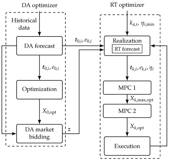
The proposed control framework is structured as a two-layer hierarchical optimization model, comprising a DA optimizer and a RT optimizer, as illustrated in Figure 1. This structure is aligned with the bidding mechanisms and operational requirements of San Diego Gas & Electric’s (SDG&E) Demand Response Auction Mechanism (DRAM), which operates within the Day-Ahead wholesale demand response market.

Figure 1. The control block diagram of the two-layer optimization model is comprised of: (1) a day ahead optimizer, which outputs the optimal EV schedule and demand response bidding price and capacity, and (2) a two-stage real-time optimizer, which optimizes the EV charging timing and energy demand (service level).

To contextualize the timeline, we define the day of the demand response event as Day-0, and the preceding day as Day-1. The DA optimizer is executed on Day-1, while the RT optimizer operates during real-time on Day-0.

The DA optimizer is responsible for generating DA cost-optimal schedules and market decisions for EV charging using forecasted EV plug-in durations and energy demands. The DA information variable for each EV i is represented as ${\mathit{t}}_{0,i}$ which is a binary vector indicating the DA forecasted plug-in status over time; $e_{0,i}$ which is the DA forecasted energy demand; and $N_0$ which is the total number of EVs forecasted to arrive. The outcome of this optimization, $X_{0,\mathrm{opt}}$, informs the bidding strategy submitted to the DA demand response market. The design complies with SDG&E requirements, including submission deadlines by 1000 h PST on Day-1. A full formulation of this optimizer and the corresponding bidding strategy is provided in Section 2.3.

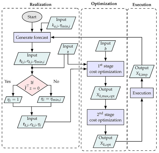
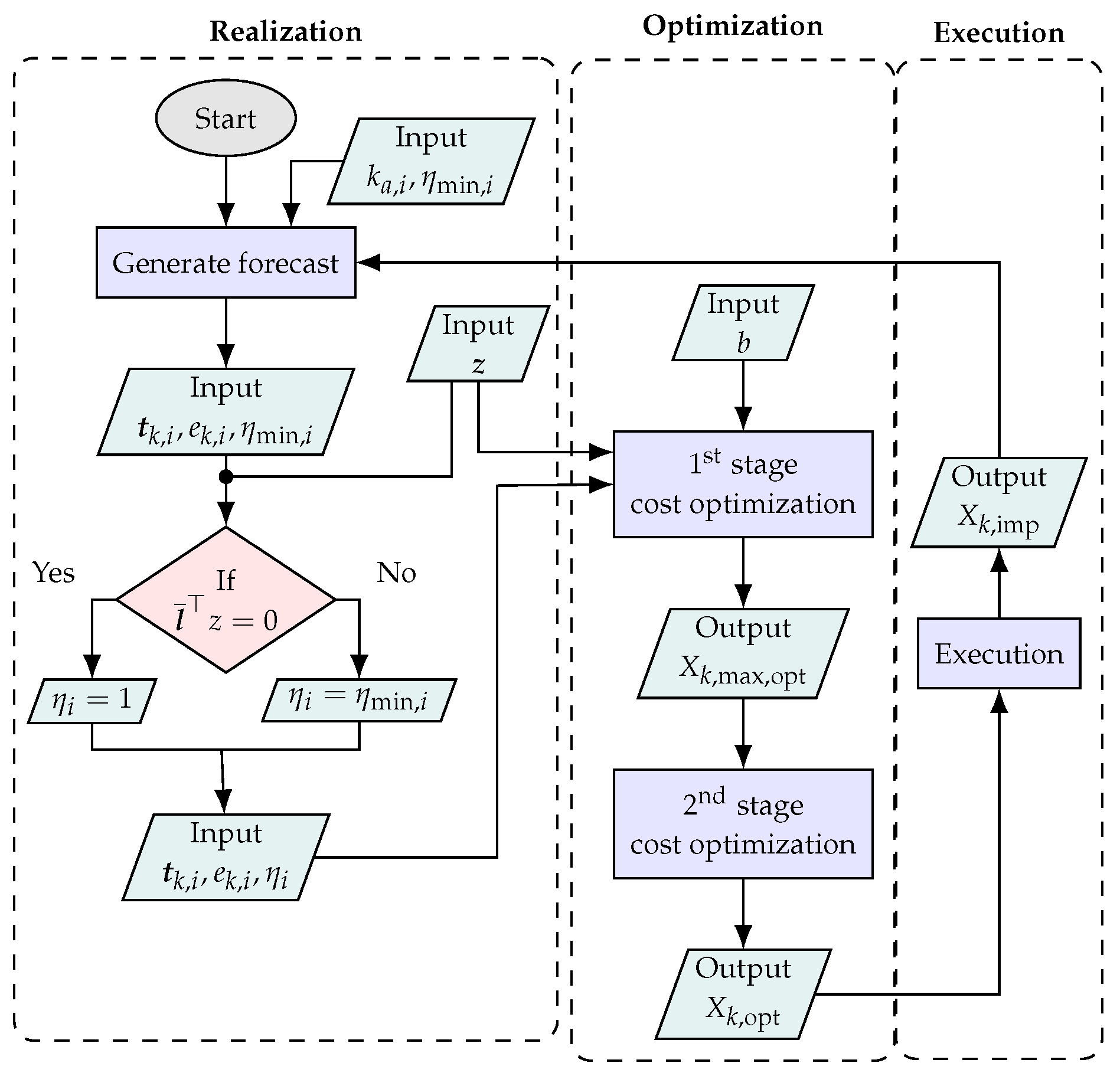
The RT optimizer functions in three sequential phases. (i) The first is the Realization phase in which the forecasted EV plug-in durations and energy demands are updated based on real-time information from newly arrived EVs. ($ii$) These updated parameters are used in the second Optimization phase, which itself proceeds in two stages. The first stage generates a schedule assuming full service level, resulting in an upper-bound solution $X_{k,\max ,\mathrm{opt}}$ at each discrete time interval k. In the second stage, the optimizer re-evaluates the schedule within a constrained range, bounded below by the user-defined minimum service levels ${\eta }_{i,\min }$ and above by $X_{k,\max ,\mathrm{opt}}$. ($iii$) This refined schedule is passed on to the third Execution phase, where only the first time step for each arrived EV is implemented. After each time step, energy demand values are updated and used as feedback into the Realization phase at the next time step. Details of this process are elaborated in Section 2.4.

2.3. DA Optimizer

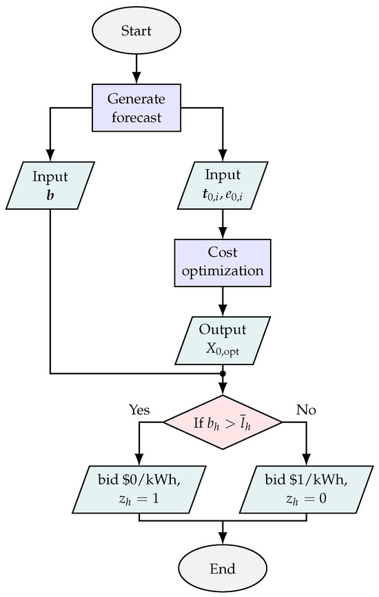
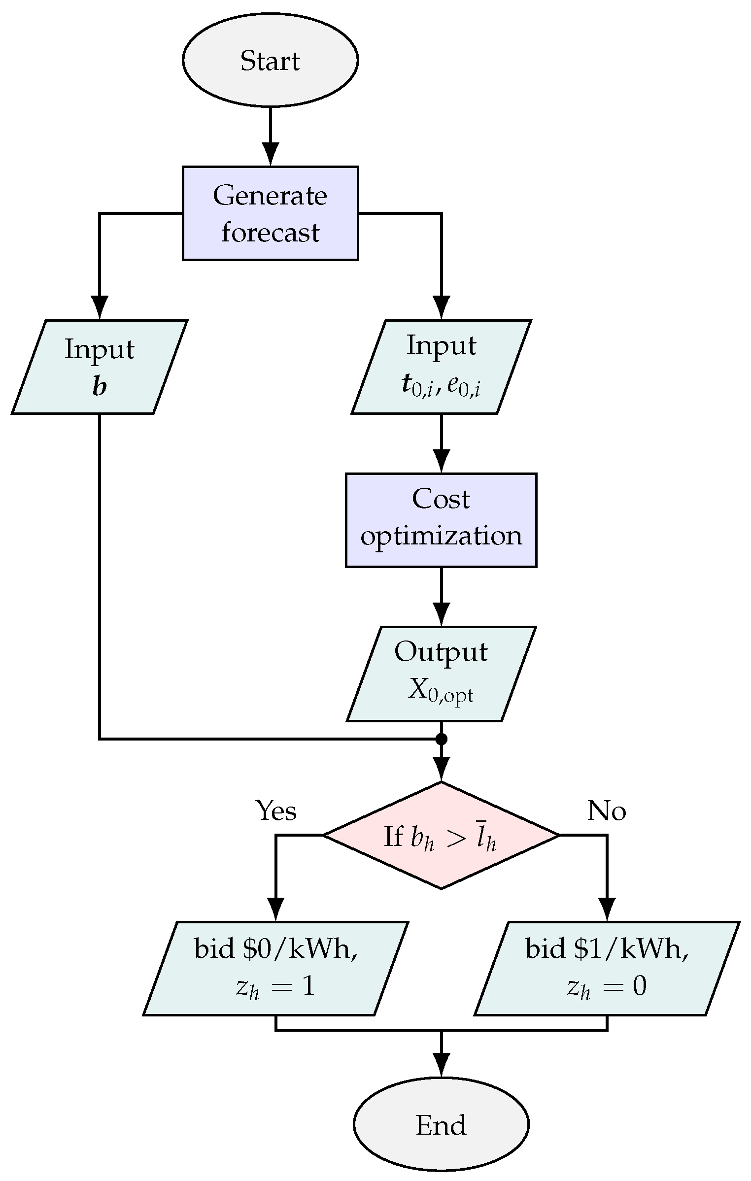
The DA optimization process begins with the forecasting of EV plug-in durations and energy demands and culminates in the determination of demand response bid prices and capacities for each hour of Day 0. The algorithm flow is depicted in Figure 2.

Figure 2. Flowchart of the DA optimizer algorithm. In the Forecasting phase, EV plug-in durations and energy demands are predicted. These forecasts are then input to the Optimization phase, which produces the cost-optimal EV charging schedule for the event day. In the final Market bidding phase, this optimized schedule is evaluated against the forecasted baseline to determine the bid price and the demand response capacity for each hour.

2.3.1. DA Forecast

Two types of forecasts are employed in the DA optimizer: perfect forecast and persistence forecast (see Section 2.6). The perfect forecast retrospectively uses actual Day-0 EV data, simulating ideal conditions. The persistence forecast relies on historical EV data from the most recent similar day: a most recent weekend or holiday if Day-1 is a weekend or holiday, or a most recent weekday otherwise.

The DA forecasts provide estimates for three key inputs: the total number of EVs expected to arrive that day, $N_0$; the EV availability matrix, $E_0$; and the energy demands of each EV, $e_{0,i}$. The EV availability matrix, shown in Table 1, is a $K\times N_0$ matrix constructed from the forecasted EV plug-in durations, that is, the $K\times 1$ binary vectors ${\mathit{t}}_{0,i}$ for each EV $i=1,\dots ,N_0$, and their respective maximum charging rates, $e_{\max ,i}$. $K=96$ is the total number of 15 minute time steps ($\Delta t$) within 24 h. The subscript 0 is added to distinguish these quantities from RT optimization variables in the next section. As illustrated in Figure 1, each column of $E_0$ represents a forecasted EV (ordered by arrival time), and each row corresponds to a discrete time interval. The EV availability matrix thus captures when each EV is expected to be available for charging as well as the maximum allowable charging rate, and serves as a structural input to the subsequent optimization process.

Table 1. Example of the EV availability matrix $E_0$ generated from day-ahead forecasts. Each column represents a forecasted EV, indexed by arrival time, and each row corresponds to a discrete time interval (here: 15 min). The non-zero regions indicate the forecasted plug-in durations during which charging is possible, constrained by the maximum charging rates (in kWh). This matrix forms a structural constraint to the scheduling optimization process.

Time Step	EV 1	EV 2	⋯	EV N
1	1.7	0	⋯	0
2	1.7	1.7	⋯	0
⋮	⋮	⋮	⋮	⋮
k	0	0	⋯	1.7

In our previous work, $N_0$ was assumed to be known with perfect foresight. In this paper, $N_0$ is estimated through the DA forecasting model. During RT operation, if the actual number of EVs at time step k exceeds the forecast ($N_0$ is under-forecasted), additional columns are appended to the real-time EV availability matrix $E_k$ to incorporate the newly arrived EVs and accommodate the charging demands. Similarly, $N_k$ is used to keep track of the updated number of EVs at every timestep. Conversely, if $N_0$ is over-forecasted, the number of columns remains unchanged, and any excess forecasted energy demand is simply not dispatched by the end of the day.

2.3.2. Optimization

The DA optimizer solves a convex cost minimization problem that includes the following components: non-coincident demand charge, ${\mathcal{C}}_{\mathrm{NCD}}(X_{0,\mathrm{opt}},h_{0,\mathrm{NCD}})$, peak-demand charge, ${\mathcal{C}}_{\mathrm{PD}}(X_{0,\mathrm{opt}},h_{0,\mathrm{PD}})$, time-of-use (TOU) energy charge, ${\mathcal{C}}_{\mathrm{TOU}}\left(X_{0,\mathrm{opt}}\right)$, and the EV service revenue, ${\mathcal{C}}_{\mathrm{EV}}\left(X_{0,\mathrm{opt}}\right)$:

$$\begin{array}{cc}\hfill \underset{X_{0,\mathrm{opt}}}{min}& {\mathcal{C}}_{\mathrm{NCD}}(X_{0,\mathrm{opt}},h_{0,\mathrm{NCD}})+{\mathcal{C}}_{\mathrm{PD}}(X_{0,\mathrm{opt}},h_{0,\mathrm{PD}})+\hfill \\ \hfill & {\mathcal{C}}_{\mathrm{TOU}}\left(X_{0,\mathrm{opt}}\right)-{\mathcal{C}}_{\mathrm{EV}}\left(X_{0,\mathrm{opt}}\right),\hfill \end{array}$$

(1)

$$\begin{array}{cc}\hfill \mathrm{s}.\mathrm{t}.& {\mathbb{1}}_K^{\top }{X}_{0,\mathrm{opt}}=(1/\Delta t){\mathit{e}}_0,\hfill \end{array}$$

(2)

$$\begin{array}{cc}\hfill & 0<X_{0,\mathrm{opt}}<(1/\Delta t)E_0\hfill \end{array}$$

(3)

where ${\mathbb{1}}_K$ is a $K\times 1$ dimensional vector of all 1, $X_{0,\mathrm{opt}}$ is the optimal charging schedule of dimension $K\times N_0$, ${\mathit{e}}_0=(e_{0,1},e_{0,2},\dots ,e_{0,N_0})$ is the energy demand vector of all $N_0$ forecasted EVs.

Historical peak demand values, $h_{0,\mathrm{NCD}}$ (non-coincident demand threshold) and $h_{0,\mathrm{PD}}$ (peak demand threshold), are incorporated into the model to account for monthly billing constraints, following [16]. At the first time step of the month, the optimizer minimizes the peak demand over 24 hours. In subsequent time steps, the optimizer tracks the existing non-coincident demand and peak demand of the month, as the thresholds $h_{0,\mathrm{NCD}}$ and $h_{0,\mathrm{PD}}$, and only attempts to reduce the demands if it exceeds the existing thresholds. The specific equations for computing demand charges, TOU costs, and EV service revenue are provided in [16].

Notably, the DA objective function excludes market revenues. This design choice is intentional: the DA optimizer is primarily used to inform market bid decisions, which are binary based on whether the forecasted load is above or below the baseline for a given hour. Including market prices would introduce noise and volatility due to their fluctuating nature. By excluding them, the DA optimizer focuses solely on the underlying load behavior, free from oscillations caused by market price differences. This also reduces forecast uncertainty and avoids reliance on speculative market price predictions.

2.3.3. DA Demand Response Market Bidding

A conservative bidding strategy, as proposed by [16], is employed in the DA demand response market bidding phase. We first define ${\mathit{l}}_{0,\mathrm{opt}}=X_{0,\mathrm{opt}}{\mathbb{1}}_{N_0}$ as the vector of total optimized EV load at 15 minute time steps, then the average hourly EV load for hour h is obtained as, ${\overline{l}}_h=(1/4){\sum }_{i=4(h-1)+1}^{4h}{l}_{0,\mathrm{opt}}\left(i\right)$ collected in the vector $\overline{\mathit{l}}$. For each hour of Day 0, if the average hourly optimized EV load is lower than the hourly baseline, $\mathit{b}={(b_1,\dots ,b_{24})}^{\top }$, that is, $b_h>{\overline{l}}_h$, then market participation is considered advantageous, and a bidding price of $0/kWh is submitted. Otherwise, a bidding price of $1/kWh is used. These prices assume that there is no opportunity cost for the market participation. So even a small positive market price is beneficial to the aggregator. This is because the forecasted load is already below the baseline, so the aggregator does not need to take any scheduling action nor communicate with the EV drivers to achieve the market revenue. In practice, there is an opportunity cost and the aggregator would factor that into the minimum bid price.

Since market clearing prices are typically below $1/kWh, submitting a $1/kWh bid effectively excludes the hour from market participation, while a $0/kWh bid typically results in a market award. Thus, the bid prices directly determine the binary vector $\mathit{z}={(z_1,\dots ,z_{24})}^{\top }$, where $z_h=1$ indicates participation in the demand response market during hour h, and $z_h=0$ indicates non-participation. Alongside the bidding price, a demand response capacity is also determined for each participating hour. This capacity is defined as the difference between the baseline and the DA-optimized EV load ($b_h-{\overline{l}}_h$), and it represents the expected demand response contribution. Although the full capacity is bid with the intention of being delivered in real time, actual revenue is settled at the end of the day based on the demonstrated load reduction, after accounting for forecast uncertainties. The detailed settlement process is described in Section 2.5.

2.4. RT Optimizer

The algorithm flowchart of the RT optimizer comprises three sequential and iterative phases: (i) the realization, ($ii$) the two-stage optimization, and ($iii$) the execution stage, which are repeated at every 15-minute time step throughout the event day, as illustrated in Figure 3. An MPC framework with a shrinking time horizon is implemented. To enable discrete-time optimization, the event day is divided into $K=96$ time steps, each of 15 minutes in duration. Here, $k=1,\dots ,K$ is used to represent the time step indices. Furthermore, all RT variables have subscript k to distinguish from DA variables with subscript 0.

Figure 3. RT optimizer flowchart. At each time step, newly arrived EV data updates the forecasts in the Realization phase. The updated inputs are used in the two-stage Optimization phase to generate feasible charging schedules. In the Execution phase, only the first time step of the schedule is implemented, and the results are fed back to update the next iteration.

At the initial iteration $k=1$ (00:00), the optimization horizon spans the entire day. As time advances, the horizon shrinks progressively. By the final iteration $k=96$ at 23:45, only a single time step remains. As overnight charging is rare, midnight serves as a convenient temporal boundary for the MPC. Correspondingly, the dimensions of all time-dependent variables, such as the EV availability matrix, $E_k$, and the EV dispatch schedule $X_{k,\mathrm{opt}}$, are updated at each iteration to reflect the reduced horizon [16].

A critical addition compared to [16] is the consideration of a service level reduction in the RT optimizer that allows the EV aggregator to explore flexibility of the EV charging energy demand to maximize demand response market revenue. To ensure the service level reduction is only applied when it leads to extra market revenue, for EVs for which the plug-in duration does not overlap with the market event hours, the service level is set to be 100%. We assume perfect foresight of the user-input service level.

2.4.1. Realization

In the Realization phase, the RT optimizer initializes EV plug-in durations (${\mathit{t}}_{k,i}$), energy demands ($e_{k,i}$), and minimum service levels (${\eta }_{\min ,i}$) at the start of the event day $k=1$ (or 00:00) using forecasts from the DA stage as,

$${\mathit{t}}_{1,i}={\mathit{t}}_{0,i},e_{1,i}=e_{0,i}.$$

As EVs arrive, these forecasts are continuously refined using real-time data from newly connected vehicles, $k_{a,i}$, and ${\eta }_{\min ,i}$, where $k_{a,i}$ is the actual arrival time. Additionally, as energy is dispatched to arrived EVs, the optimizer incorporates feedback from the execution phase to further update the inputs. These updates improve the system’s awareness of evolving charging needs and operational constraints. Unlike the static DA forecasts based on historical patterns, the RT forecasts are dynamic, leveraging real-time arrival times, user identifiers, battery specifications, and minimum service levels for more accurate estimation of plug-in durations and energy requirements.

Three types of forecasting methods are considered within the RT optimizer: perfect forecast, persistence forecast, and linear regression (LR) forecast (see Section 2.6). The perfect forecast and the persistence forecast are discussed in Section 2.3.1. For the LR forecast, a rule-based method is used for known users based on the past sessions’ features and the current arrival time, and a weighted linear regression approach is used for unknown users based on the weekday, the maximum charging power, and the arrival time of the current session.

To prepare inputs for the upcoming optimization phase, the EV availability matrix, $E_k$, inherited from the DA optimizer is progressively updated. As each EV arrives, its corresponding column in the matrix is replaced with updated availability information, preserving the original chronological order of arrival. The DA energy demand forecast for each EV is replaced by the RT forecasted energy demand, $e_{k,i}$, upon EV arrival, and is updated iteratively based on the dispatched energy from the execution phase of the previous time step, $X_{k-1,\mathrm{imp}}$.

2.4.2. Optimization

In the two-stage optimization phase, the system optimizes both the timing and magnitude of EV charging. In the first stage, the optimizer assumes full service levels for all EVs and computes an upper-bound solution that reflects maximum service delivery under current system constraints. In the second stage, the optimization is re-executed with additional constraints that enforce user-defined minimum service levels. This refinement yields a feasible and cost-effective charging schedule that balances user satisfaction with the potential market revenue gained by reducing service levels.

In the first stage of this optimization, the objective function closely mirrors that of the DA optimizer but includes an additional term to capture market revenue as,

$$\begin{array}{cc}\hfill \underset{X_{k,\max ,\mathrm{opt}}}{min}& {\mathcal{C}}_{\mathrm{NCD}}(X_{k,\max ,\mathrm{opt}},h_{k,\mathrm{NCD}})+{\mathcal{C}}_{\mathrm{PD}}(X_{k,\max ,\mathrm{opt}},h_{k,\mathrm{PD}})+\hfill \\ \hfill & {\mathcal{C}}_{\mathrm{TOU}}\left(X_{k,\max ,\mathrm{opt}}\right)-{\mathcal{C}}_{\mathrm{EV}}\left(X_{k,\max ,\mathrm{opt}}\right)-\hfill \\ \hfill & {\mathcal{C}}_{\mathrm{DR}}(X_{k,\max ,\mathrm{opt}},\mathit{b},\mathit{z}),\hfill \end{array}$$

(4)

$$\begin{array}{cc}\hfill \mathrm{s}.\mathrm{t}.& {\mathbb{1}}_{(K-k)}^{\top }{X}_{k,\max ,\mathrm{opt}}=(1/\Delta t){\mathit{e}}_k,\hfill \end{array}$$

(5)

$$\begin{array}{cc}\hfill & 0<X_{k,\max ,\mathrm{opt}}<(1/\Delta t)E_k.\hfill \end{array}$$

(6)

Specifically, the demand response market revenue, denoted as ${\mathcal{C}}_{\mathrm{DR}}(X_{k,\max ,\mathrm{opt}},\mathit{b},\mathit{z})$, is calculated based on the difference between the baseline load profile $\mathit{b}$ and the optimized EV load, along with the designated event hours $\mathit{z}$. Equation (5) ensures full service level fulfillment, that is, ${\eta }_i=1$.

This stage yields a schedule trajectory ${\mathit{l}}_{\max ,\mathrm{opt}}=X_{k,\max ,\mathrm{opt}}{\mathbb{1}}_{N_k}$, which reflects the revenue potential under maximum service level conditions. This trajectory serves as a reference trajectory, and the service level as an upper bound of energy demands in the second optimization stage.

In the second stage, flexibility in EV charging energy demand is introduced by relaxing the strict energy delivery requirement. The model allows flexibility by applying inequality constraints that ensure the total delivered energy lies between the user-defined minimum service level ${\eta }_{\min ,i}$ and 100% of the original energy demand. This approach enables the system to strategically reduce energy delivery within acceptable bounds to pursue potential gains from market participation, while still respecting user-defined service guarantees.

$$\begin{array}{cc}\hfill \underset{X_{k,\mathrm{opt}}}{min}& {\mathcal{C}}_{\mathrm{NCD}}(X_{k,\mathrm{opt}},h_{k,\mathrm{NCD}})+{\mathcal{C}}_{\mathrm{PD}}(X_{k,\mathrm{opt}},h_{k,\mathrm{PD}})+\hfill \\ \hfill & {\mathcal{C}}_{\mathrm{TOU}}\left(X_{k,\mathrm{opt}}\right)-{\mathcal{C}}_{\mathrm{EV}}\left(X_{k,\mathrm{opt}}\right)-\hfill \\ \hfill & {\mathcal{C}}_{\mathrm{DR}}(X_{k,\mathrm{opt}},\mathit{b},\mathit{z})+{\mathcal{C}}_{\mathrm{track}}(X_{k,\mathrm{opt}},{\mathit{l}}_{\max ,\mathrm{opt}},\mathit{z}),\hfill \end{array}$$

(7)

$$\begin{array}{cc}\hfill \mathrm{s}.\mathrm{t}.& (1/\Delta t){\mathcal{E}}_{\min }(e_{k,i},X_{k-1,\mathrm{imp}},{\eta }_i)<=X_{k,\mathrm{opt}}{\mathbb{1}}_{N_k}\hfill \\ \hfill & <=(1/\Delta t){\mathcal{E}}_{\max }(e_{k,i},X_{k-1,\mathrm{imp}}),\hfill \end{array}$$

(8)

$$\begin{array}{cc}\hfill & 0<X_{k,\mathrm{opt}}<(1/\Delta t)E_k,\hfill \end{array}$$

(9)

where ${\eta }_i={\eta }_{\min ,i}$ if the layover period of EV i overlaps with market participation hours $z_h=1$. By exploiting this flexibility, the EV aggregator can maximize revenue and reconcile mismatches between DA bidding commitments and real-time availability, which often arises due to forecast uncertainty. The actual service level for each EV is determined by the optimization outcome at each step and can be evaluated retrospectively at the end of the day. ${\mathcal{E}}_{\max }(e_{k,i},X_{k-1,\mathrm{imp}})$ and ${\mathcal{E}}_{\min }(e_{k,i},X_{k-1,\mathrm{imp}},{\eta }_i)$ are the upper and lower bounds of the energy demand corresponding to the $100\%$ and ${\eta }_i$ service level.

In real-world demand response markets, the revenue is not only a function of the current day’s EV load but also influenced by historical consumption patterns that are manifested in the baseline. A lower EV load on a given day reduces the baseline for subsequent days, potentially diminishing future market revenues. To mitigate this effect, the proposed model restricts service level reductions to demand response event hours only. However, since energy dispatch is time-coupled and service reductions cannot be predetermined, direct enforcement is not feasible. Instead, a trajectory tracking quadratic penalty term, ${\mathcal{C}}_{\mathrm{track}}(X_{k,\mathrm{opt}},{\mathit{l}}_{\max ,\mathrm{opt}},\mathit{z})$, is added to the objective function. This term penalizes deviations from the full-service trajectory $\mathit{l}$ during non-event hours, effectively discouraging reductions outside of event windows. As a result, service level reductions are concentrated during market events, preserving baseline integrity across days.

2.4.3. Execution

In the Execution phase, only the first time step of the optimized dispatch schedule is implemented. To track the actual energy dispatched to each EV in real time, an implemented matrix $X_{k,\mathrm{imp}}$ of dimension $k\times N_k$ is constructed, as illustrated in Table 2. The implemented matrix has no columns at the start of the day and expands as more EVs arrive. As time k advances, the implemented matrix grows. Similarly, the EV availability matrix $E_k$ with dimension $(K-k)\times N_k$ shrinks accordingly. The number of columns in the EV availability matrix may increase if the number of arriving EVs, $N_k$, was under-forecasted as explained earlier.

Table 2. An example of the output matrices $X_{k,\mathrm{opt}}$ and $X_{k,\max ,\mathrm{opt}}$ (top), and the implemented matrix $X_{k,\mathrm{imp}}$ (bottom) at time k during real-time execution, assuming only $N_k\le N_K$ EVs arrived at k, where $N_K$ is actual number of arrived EVs.

Time step	EV 1	EV 2	⋯	EV $N_k$	…	EV $N_K$
k	1.7	1.7	⋯	0	⋯	0
$k+1$	1.7	1.7	⋯	0	⋯	0
⋮	⋮	⋮	⋮	⋮	⋮	⋮
K	0	0	⋯	1.7	⋯	1.7
Time step	EV 1	EV 2	⋯	EV $N_k$
1	1.7	0	⋯	0
2	1.7	1.7	⋯	0
⋮	⋮	⋮	⋮	⋮
k	1.7	1.7	⋯	0

After implementing the scheduled dispatch, the updated implemented matrix is then fed back into the Realization phase, enabling the RT optimizer to adapt iteratively to the system’s evolving state throughout the day.

2.4.4. Algorithm

Algorithm 1 shows the proposed Two-stage RT optimizer.

Algorithm 1 Proposed Two-stage RT Optimizer

1: Initialize $E_0$ and $e_{0,i}$.   2: Define the arrival time $k_{a,i}$ for EV i   3: for $k\in \{1,\dots ,K\}$ do    Realization phase   4:    for EV i with $k_{a,i}=k-1$ do   5:        Obtain $e_{\max ,i}$   6:        Forecast ${\mathit{t}}_{k,i}$ and $e_{k,i}$   7:    end for   8:    Update $E_k$ based on ${\mathit{t}}_{k,i}$ and $e_{\max ,i}$ for all EVs with $k_{a,i}=k-1$   9:    Update $e_{k,i}$ with actual energy demand for all EVs with $k_{a,i}=k-1$ 10:    Update $e_{k,i}$ based on $X_{k-1,\mathrm{opt}}$ for all EVs with $k_{a,i}<k-1$    Two-stage optimization phase 11:    Solve the optimization problem to get the output $X_{k,\mathrm{opt}}$, per Equations (4)–(6) 12:    Generate upper and lower bounds ${\mathcal{E}}_{\max }(e_{k,i},X_{k,\mathrm{opt}})$, ${\mathcal{E}}_{\min }(e_{k,i},X_{k,\mathrm{opt},{\eta }_i})$ 13:    Re-solve the optimization problem to get the final output $X_{k,\mathrm{opt}}$, per Equations (7)–(9)    Execution phase 14:    Implement the first time step of $X_{k,\mathrm{opt}}$ 15: end for

2.5. Market Settlement

In the DA demand response market, participants earn revenue through two streams: capacity revenue and energy revenue. Capacity revenue, which is proportional to the bid demand reduction capacity, is not included in the optimization algorithm or revenue analysis in this study; further details are provided in [31]. Energy revenue, on the other hand, is based on the actual demonstrated demand reduction, $X_{k,\mathrm{imp}}$, and is composed of two components: the DA settlement ($s_{\mathrm{DA}}$) and the RT settlement ($s_{\mathrm{RT}}$).

The DA settlement compensates the ability to deliver the committed demand reduction under forecast uncertainty. It is calculated as the product of the DA Locational Marginal Price (LMP) and the realized demand reduction, bounded between zero and the bid capacity. The RT settlement adjusts for any deviation from the committed capacity. It rewards or penalizes the over- or under-performance of demand reduction at the RT LMP. However, the penalty is capped such that it does not exceed the originally bid demand reduction capacity. In other words, the worst case scenario is zero revenue from demand response market participation. Details are discussed in [16].

2.6. Case Study

2.6.1. EV Charging Site

The proposed optimization model was evaluated using 2022 EV charging data collected from PowerFlex V1G EV chargers deployed on the UC San Diego campus. The charging infrastructure includes five Tesla chargers, each rated at a maximum power capacity of 10.3 kW, and 46 AeroVironment/Webasto DX chargers, each with a maximum power capacity of 6.7 kW.

These chargers are distributed across two charging plazas: the Gilman Parking Structure, a typical workplace charging site, and the Athena Parking Garage, which serves nearby medical facilities. The latter exhibits a more diverse charging pattern due to the presence of medical staff working 12-h shifts and short-stay visitors with brief charging needs.

In total, 502,023 charging sessions were recorded at these two sites over the course of 2022, including 780 sessions in December, providing a comprehensive dataset for validating the model’s performance under real-world conditions.

2.6.2. Computational Setup

The simulation was implemented in Python 3.10, utilizing the CVXPY optimization library to solve the dispatch problem. All experiments were conducted on a machine equipped with an Intel Core i7-4790 CPU @ 3.60 GHz and 32.0 GB of RAM. Under this configuration, simulating one month of EV charging dispatch required approximately 14 min for all forecast scenarios, demonstrating the model’s computational efficiency for large-scale, real-world datasets.

2.7. Forecast Scenarios

The two forecast methods used in the DA optimizer are paired with the three forecast methods in the RT optimizer to form three forecast scenarios evaluated in this study:

2.7.1. Perfect Forecast (PFCT) Scenario

In this scenario, both the DA and RT optimizers are assumed to have perfect foresight of EV plug-in durations and energy demands on Day 0. This serves as an ideal benchmark for evaluating forecast-based scenarios.

2.7.2. Persistence Forecast (PSIS) Scenario

Here, both DA and RT optimizers rely on data from the most recent same day type prior to Day 0. If Day 0 is a Wednesday, for instance, the RT optimizer uses data from Tuesday, while the DA optimizer, run on Tuesday without access to Tuesday’s EV data, uses data from Monday. For a Monday Day 0, the most recent available similar day is the previous Friday. EV plug-in duration and energy demand are assumed to be known upon EV arrival.

2.7.3. Persistence + Linear Regression Forecast (PSIS-LR) Scenario

This scenario builds upon the PSIS setup but reflects a more realistic setting where EV departure time and energy demand are not known upon arrival and are instead forecasted using a LR model. The LR method is discussed in Section 2.4.1.

2.8. Simulated Charging Cases

To evaluate the performance of the proposed model, several benchmark scenarios are simulated:

2.8.1. $\mathrm{V}0{\mathrm{G}}_{100\%}$—Dumb Charging Case

In this scenario, all EVs are charged immediately upon arrival at their maximum charging rate, without any control or scheduling. This results in an unmanaged EV load profile and serves as a reference for comparison with the managed charging strategies described below.

2.8.2. $\mathrm{V}1{\mathrm{G}}_{\mathrm{real},100\%}$—Real PowerFlex Controlled Charging

This scenario reflects the actual EV load profile observed on the day, using the PowerFlex control algorithm. The algorithm applies a set of predefined charging rate limits throughout the day to prevent significant demand peaks while still ensuring full EV service levels.

2.8.3. $\mathrm{V}1{\mathrm{G}}_{\mathrm{opt},\mathrm{imp},100\%}$—Optimized Charging with Full Service Level

To assess the economic benefits of leveraging EV flexibility for demand response market participation, a base case is defined. It uses the same DA optimization as the proposed method (see Equations (1)–(3)) but limits the RT optimization to its first stage only (see Equations (4)–(6)). In this case, EV charging schedules are optimized while maintaining 100% service levels, i.e., without any reduction in EV energy demand.

2.8.4. ${\mathrm{V}1\mathrm{G}}_{\mathrm{opt},\mathrm{imp},\eta }$—Proposed Method with RT Energy Demand Flexibility

This scenario implements the full proposed method, allowing EV service levels to be adjusted in real time to increase market revenue. The actual level of service, denoted by $\eta$, is not predetermined and is calculated retrospectively as the ratio of actual dispatched energy to the total energy demand.

For the user-defined minimum service level ${\eta }_{\min ,i}$, it is assumed that users specify their minimum acceptable service level upon arrival. Since this information is not directly available in the dataset, we model it using a synthetic distribution: 10% of users have ${\eta }_{\min ,i}=100\%$, 60% have ${\eta }_{\min ,i}=80\%$, and the remaining 30% are evenly split among ${\eta }_{\min ,i}=60\%$, $40\%$, and $20\%$. The service-level distribution was chosen ad-hoc as we were not aware of any data that supports an empirical distribution. The impact of the service-level distribution is that cars with a smaller minimal service level would have more flexibility which would result in a larger revenue potential.

2.9. Baseline Initiation

The baselines for the two optimal cases, $\mathrm{V}1{\mathrm{G}}_{\mathrm{opt},\mathrm{imp},100\%}$ and ${\mathrm{V}1\mathrm{G}}_{\mathrm{opt},\mathrm{imp},\eta }$, are denoted as ${\mathrm{baseline}}_{100\%}$ and ${\mathrm{baseline}}_{\eta }$, respectively. To construct these baselines, the DA optimizer simulates the optimal EV load profile for the year 2022, up to 30 November. The demand response market participation is assumed to begin on 1 December 2022. Consequently, the implemented load profiles for both $\mathrm{V}1{\mathrm{G}}_{\mathrm{opt},\mathrm{imp},100\%}$ and ${\mathrm{V}1\mathrm{G}}_{\mathrm{opt},\mathrm{imp},\eta }$ are identical before this date, leading to identical initial baselines.

From 2 December onward, ${\mathrm{V}1\mathrm{G}}_{\mathrm{opt},\mathrm{imp},\eta }$ reflects reduced service levels due to demand response market participation, resulting in a lower implemented load. Without intervention, this would cause ${\mathrm{baseline}}_{\eta }$ to shift downward, thereby decreasing potential future market revenues. To mitigate this, we introduce a penalty term in the objective function (Equation (7)), which minimizes deviation from ${\mathrm{baseline}}_{100\%}$ during non-event hours. This encourages demand reduction to occur primarily during event hours, preserving the baseline trajectory while enabling revenue generation through demand response participation, as detailed in Section 1 and Section 2.4.2.

The choice to simulate a common implemented load profile for both $\mathrm{V}1{\mathrm{G}}_{\mathrm{opt},\mathrm{imp},100\%}$ and ${\mathrm{V}1\mathrm{G}}_{\mathrm{opt},\mathrm{imp},\eta }$ up to the start of market participation on 1 December 2022, allows for the use of a shared initial baseline. This design enables a controlled analysis of how demand response participation affects baseline dynamics and revenue, by isolating the impact of reduced service levels post-December 1.

While an alternative approach would involve independently simulating and establishing separate baselines for each scenario over several months, such a method introduces confounding effects due to baseline drift and other cumulative changes, making it harder to attribute differences in performance solely to demand response participation. Our strategy is motivated by practical considerations around baseline availability in real-world implementations. Many baseline methodologies, including those used by utilities and ISOs, rely on the availability of recent non-event days to calculate reference loads. However, for aggregators or customers with high market participation rates, identifying a sufficient number of recent non-event days can be challenging. Some utilities address this by extending the historical window or relaxing requirements, but specific rules vary. In our study, we assume no strict limitation on the recency of baseline days, making the simulation results scalable over longer periods. This assumption supports the feasibility of preserving the baseline trajectory through a penalty mechanism that discourages load reduction outside of event hours, as introduced in Equation (7) and discussed in Section 1 and Section 2.4.2.

3. Results and Discussion

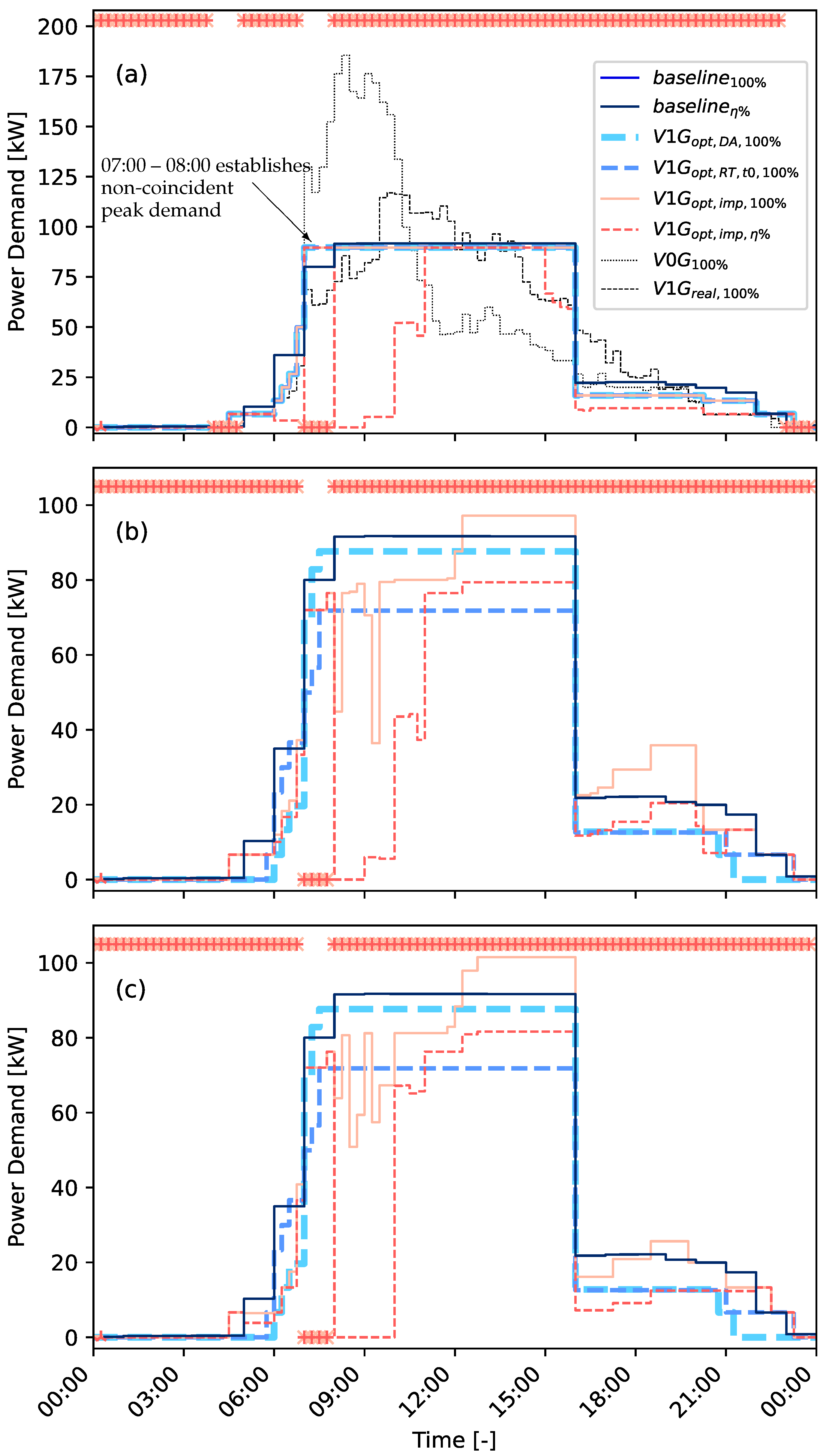
3.1. Daily Optimized Profile with PFCT Forecast (Figure 4a)

Figure 4a presents the simulation results for 1 December 2022, including: (1) the optimal EV load profile from the DA optimizer; (2) the corresponding bidding price and event hour identification; and (3) the optimal RT EV load profile, generated using perfect foresight.

Figure 4. Optimized EV charging profiles and market event hour indicators on 1 December 2022, under (a) PFCT forecast, (b) PSIS forecast, and (c) PSIS-LR forecast: comparison of DA ($\mathrm{V}1{\mathrm{G}}_{\mathrm{opt},\mathrm{DA},100\%}$, thick dashed light blue) and RT ($\mathrm{V}1{\mathrm{G}}_{\mathrm{opt},\mathrm{RT},100\%}$, thin dashed dark blue) optimization results with full and partial service levels ($\mathrm{V}1{\mathrm{G}}_{\mathrm{opt},\mathrm{imp},100\%}$ and ${\mathrm{V}1\mathrm{G}}_{\mathrm{opt},\mathrm{imp},\eta }$, solid and dashed red lines), and unmanaged charging ($\mathrm{V}0{\mathrm{G}}_{100\%}$). The baselines for full and partial service levels are shown as dark blue solid (baseline_100%) and black solid (baseline_η) lines.

Figure 4. Optimized EV charging profiles and market event hour indicators on 1 December 2022, under (a) PFCT forecast, (b) PSIS forecast, and (c) PSIS-LR forecast: comparison of DA ($\mathrm{V}1{\mathrm{G}}_{\mathrm{opt},\mathrm{DA},100\%}$, thick dashed light blue) and RT ($\mathrm{V}1{\mathrm{G}}_{\mathrm{opt},\mathrm{RT},100\%}$, thin dashed dark blue) optimization results with full and partial service levels ($\mathrm{V}1{\mathrm{G}}_{\mathrm{opt},\mathrm{imp},100\%}$ and ${\mathrm{V}1\mathrm{G}}_{\mathrm{opt},\mathrm{imp},\eta }$, solid and dashed red lines), and unmanaged charging ($\mathrm{V}0{\mathrm{G}}_{100\%}$). The baselines for full and partial service levels are shown as dark blue solid (baseline_100%) and black solid (baseline_η) lines.

3.1.1. Results from the DA Optimizer

$\mathrm{V}1{\mathrm{G}}_{\mathrm{opt},\mathrm{DA},100\%}$ represents the cost-optimal EV scheduling result from the DA optimizer. This profile serves as the DA forecasted EV load and is used to determine market bidding decisions by comparing it against the baselines, ${\mathrm{baseline}}_{100\%}$ and ${\mathrm{baseline}}_{\eta }$. As noted in Section 2.9, these two baselines are identical on December 1.

3.1.2. Bidding Price and Event Hour Identification

As described in Section 2.3.3, a bidding price of $0/kWh is submitted during hours when the baseline exceeds the DA forecasted load—these are designated as event hours (marked at the top of the graph). In contrast, when the DA forecasted load is higher than the baseline, the corresponding hour is labeled a non-event hour (marked at the bottom). On 1 December, the baselines exceed the forecasted load ($\mathrm{V}1{\mathrm{G}}_{\mathrm{opt},\mathrm{imp},100\%}$) for all hours except 04:00–05:00, 07:00–08:00, and 23:00–24:00, which are identified as non-event hours.

3.1.3. Results from the RT Optimizer

The optimal charging case with full service level, $\mathrm{V}1{\mathrm{G}}_{\mathrm{opt},\mathrm{imp},100\%}$ (orange line), incorporates market revenue into its objective function. As shown in Figure 4a, the resulting profile closely overlaps with the DA forecasted profile, $\mathrm{V}1{\mathrm{G}}_{\mathrm{opt},\mathrm{DA},100\%}$, throughout the entire day, despite the inclusion of the market revenue term. This similarity arises because demand charges are the dominant component of the total cost. Although the optimizer could, in theory, adjust the load to capture market price signals, doing so would result in a net cost increase: the potential gain from market revenue is significantly outweighed by the rise in demand charges. In particular, during the plateau hours from 07:00 to 16:00, the price incentives offered by the market are not sufficient to justify dispatching a higher load than the DA optimal schedule.

$\mathrm{V}1{\mathrm{G}}_{\mathrm{opt},\mathrm{RT},\mathrm{t}0,100\%}$ represents the optimal EV load profile computed at time step $k=1$ by the RT optimizer. As described in Section 2.4.2, the RT optimizer uses an MPC framework, where each time step produces an output dispatch matrix. Under perfect forecast conditions, the dispatch matrix from the first time step ($\mathrm{V}1{\mathrm{G}}_{\mathrm{opt},\mathrm{RT},\mathrm{t}0,100\%}$) should match the final implemented dispatch matrix for the entire day ($\mathrm{V}1{\mathrm{G}}_{\mathrm{opt},\mathrm{imp},100\%}$). This alignment is confirmed in Figure 4a.

The reduced service level case, ${\mathrm{V}1\mathrm{G}}_{\mathrm{opt},\mathrm{imp},\eta }$ (dashed red line), follows the same load trajectory as $\mathrm{V}1{\mathrm{G}}_{\mathrm{opt},\mathrm{imp},100\%}$ during non-event hours, as intended by the baseline preservation strategy. During event hours, significant load reduction is observed in time slots with higher DA LMPs, while time slots with lower DA LMPs exhibit load values similar to, but not exceeding, those in the $\mathrm{V}1{\mathrm{G}}_{\mathrm{opt},\mathrm{imp},100\%}$ case. Notably, during the non-event hour from 07:00 to 08:00, the load for ${\mathrm{V}1\mathrm{G}}_{\mathrm{opt},\mathrm{imp},\eta }$ is set equal to that of $\mathrm{V}1{\mathrm{G}}_{\mathrm{opt},\mathrm{imp},100\%}$. This hour establishes the day’s non-coincident peak demand, initially 0 kW (highlighted in Figure 4a) at the start of the month, as detailed in Section 2.3.2. This threshold limits the upper bound for oscillatory load dispatch during the remainder of the day and helps to control demand charges.

Lastly, $\mathrm{V}0{\mathrm{G}}_{100\%}$ and $\mathrm{V}1{\mathrm{G}}_{\mathrm{real},100\%}$ are included in Figure 4 for comparison against the cost-optimal cases. As expected, the unmanaged EV charging profile, $\mathrm{V}0{\mathrm{G}}_{100\%}$ (dotted gray line), exhibits a pronounced peak in the morning hours when vehicles begin charging upon arrival—consistent with a typical weekday pattern. In contrast, $\mathrm{V}1{\mathrm{G}}_{\mathrm{real},100\%}$ (dotted black line), which uses preset dispatch thresholds, effectively mitigates this peak by deferring charging events to later in the day. All four cases are evaluated in terms of daily cost performance in Section 3.4.

3.2. Daily Optimized Profile with PSIS Forecast (Figure 4b)

On 1 December, when using the PSIS forecast without perfect foresight, the RT optimizer underestimates EV load, resulting in a lower projected load (dark blue dashes) in the morning hours. As more EVs arrive later in the day and provide actual energy demand information, the optimizer responds by increasing the dispatch accordingly, resulting in a higher overall load later in the day (red line). This leads to a higher non-coincident peak demand compared to the perfect foresight case.

As discussed in Section 2.7.2, the DA forecast is always generated using data from the most recent day similar to Day-1, and the RT forecast is based on data from the most recent day similar to Day-0. Because December 1 falls on a Thursday, the corresponding similar days used for forecasting in this case are Tuesday (for DA) and Wednesday (for RT). As a result, the DA forecasted total energy demand differs from the RT forecasted total energy demand. This difference is reflected in the area under the load profiles for the $\mathrm{V}1{\mathrm{G}}_{\mathrm{opt},\mathrm{DA},100\%}$ and $\mathrm{V}1{\mathrm{G}}_{\mathrm{opt},\mathrm{RT},\mathrm{t}0,100\%}$ scenarios shown in Figure 4b. In contrast, the total energy demand remains consistent across the unmanaged case ($\mathrm{V}0{\mathrm{G}}_{100\%}$), the threshold-based control case ($\mathrm{V}1{\mathrm{G}}_{\mathrm{real},100\%}$), and the cost-optimal case ($\mathrm{V}1{\mathrm{G}}_{\mathrm{opt},\mathrm{imp},100\%}$).

3.3. Daily Optimized Profile with PSIS-LR Forecast (Figure 4c)

The results obtained using the PSIS-LR forecast are close to those from the PSIS forecast, indicating that the linear regression model produces a reliable forecast for the EV load.

3.4. Daily Cost Analysis

The daily cost outcomes for 1 December 2022, are summarized in Table 3. All three forecast scenarios, PFCT, PSIS, and PSIS-LR, are evaluated under both full-service and reduced-service levels, yielding six scenarios: $\mathrm{V}1{\mathrm{G}}_{100\%,\mathrm{PFCT}}$, ${\mathrm{V}1\mathrm{G}}_{\eta ,\mathrm{PFCT}}$, $\mathrm{V}1{\mathrm{G}}_{100\%,\mathrm{PSIS}}$, ${\mathrm{V}1\mathrm{G}}_{\eta ,\mathrm{PSIS}}$, $\mathrm{V}1{\mathrm{G}}_{100\%,\mathrm{PSIS}\text{-}\mathrm{LR}}$, and ${\mathrm{V}1\mathrm{G}}_{\eta ,\mathrm{PSIS}\text{-}\mathrm{LR}}$. These correspond to the $\mathrm{V}1{\mathrm{G}}_{\mathrm{opt},\mathrm{imp}}$ profiles presented in Figure 4a–c, under their respective forecast and service-level conditions.

Table 3. Daily cost analysis with different forecasts on 1 December 2022.

Cases	Energy Demand [kWh]	TOU [$]	EV Service Revenue [$]	DA Settlement [$]	RT Settlement [$]	Net Revenue (EV + DA + RT − TOU) [$]	Net Revenue Rate [$/kWh]
$\mathrm{V}1{\mathrm{G}}_{100\%,\mathrm{PFCT}}$	944	102	142	12	$\phantom{1}$1	$\phantom{1}$52	-
${\mathrm{V}1\mathrm{G}}_{\eta ,\mathrm{PFCT}}$	640	69	$\phantom{1}$96	12	65	103	0.17
$\mathrm{V}1{\mathrm{G}}_{100\%,\mathrm{PSIS}}$	944	103	142	$\phantom{1}$7	−1	$\phantom{1}$44	-
${\mathrm{V}1\mathrm{G}}_{\eta ,\mathrm{PSIS}}$	640	$\phantom{1}$70	$\phantom{1}$96	14	51	$\phantom{1}$91	0.15
$\mathrm{V}1{\mathrm{G}}_{100\%,\mathrm{PSIS}\text{-}\mathrm{LR}}$	927	101	139	$\phantom{1}$8	$\phantom{1}$1	$\phantom{1}$47	-
${\mathrm{V}1\mathrm{G}}_{\eta ,\mathrm{PSIS}\text{-}\mathrm{LR}}$	641	$\phantom{1}$69	$\phantom{1}$96	18	52	$\phantom{1}$97	0.18

3.4.1. Energy Demand (ED)

Both $\mathrm{V}1{\mathrm{G}}_{100\%,\mathrm{PFCT}}$ and $\mathrm{V}1{\mathrm{G}}_{100\%,\mathrm{PSIS}}$ exhibit the same total energy demand, as both scenarios assume accurate knowledge of each EV’s departure time and energy requirement at the moment of arrival. In contrast, $\mathrm{V}1{\mathrm{G}}_{100\%,\mathrm{PSIS}\text{-}\mathrm{LR}}$ relies on LR-based predictions for these parameters. Due to forecast errors, some charging sessions have underforecasted energy demand targets, leading to insufficient demand charge dispatch, or overestimated plug-in durations, causing early EV departures before meeting the energy requirement. Both factors contribute to a slight reduction in total energy delivered. The final service level per EV, defined as the ratio of delivered energy to actual energy demand, varies between the user-defined minimum (${\eta }_{\min ,i}$) and 1. In the reduced-service cases (${\mathrm{V}1\mathrm{G}}_{\eta ,\mathrm{PFCT}}$, ${\mathrm{V}1\mathrm{G}}_{\eta ,\mathrm{PSIS}}$, and ${\mathrm{V}1\mathrm{G}}_{\eta ,\mathrm{PSIS}\text{-}\mathrm{LR}}$), energy demand is substantially lower. This results from strategically optimizing RT EV flexibility, specifically by reducing the service level during event hours to increase market revenues.

3.4.2. Time-of-Use (TOU) Cost

The TOU cost for $\mathrm{V}1{\mathrm{G}}_{100\%,\mathrm{PSIS}}$ exceeds that of $\mathrm{V}1{\mathrm{G}}_{100\%,\mathrm{PFCT}}$ due to a forecast-induced underestimation of morning demand. This causes the optimizer to defer a significant portion of the load to later hours, particularly into the 16:00–21:00 window when TOU rates are highest. The delayed charging, therefore, incurs greater TOU expenses relative to the perfectly forecasted schedule.

3.4.3. EV Service Revenue

The EV service revenue is directly proportional to the energy delivered, based on a fixed user charge of $0.15/kWh. As a result, scenarios with higher energy delivery (i.e., full-service cases) yield higher revenue, while reduced-service cases correspondingly generate less.

3.4.4. Market Settlement

Under perfect foresight (PFCT), both the full-service and reduced-service cases secure identical DA settlements of $12, as the DA capacity bid is fully demonstrated in real time. The reduced-service case yields higher RT settlement due to overperformance in demand reduction, earning $65 compared to just $1 for the full-service case.

Under the PSIS forecast, the full-service case is negatively impacted by forecast inaccuracies that lead to under-delivery of the DA capacity bid. As shown in Figure 4b, the DA bid capacity, defined as the difference between the baseline and $\mathrm{V}1{\mathrm{G}}_{\mathrm{opt},\mathrm{DA},100\%}$, is not fully demonstrated in RT after 12:00 h, as the actual dispatch ($\mathrm{V}1{\mathrm{G}}_{\mathrm{opt},\mathrm{imp},100\%}$) significantly exceeds the DA forecast. This results in a reduced DA settlement and incurs RT penalties for underperformance, leading to a negative RT settlement of $-1. In contrast, the reduced-service case mitigates this financial loss by lowering load during event hours. This allows for full demonstration of the DA bid during most event-hours, raising the DA settlement to $14, and further yields an RT payment of $51 due to overperformance.

A similar trend is observed in the PSIS-LR case. While the LR model introduces moderate forecast error, the reduced-service strategy again compensates by enhancing both DA and RT settlements. This demonstrates that flexible service level can serve as effective hedges against forecast uncertainty.

3.4.5. Net Revenue

Across all three forecast scenarios, the reduced-service cases yield approximately double the net revenue compared to their full-service counterparts. Here, net revenue is defined as the sum of EV service revenue and market settlements, minus the TOU cost. To quantify the economic efficiency of service reduction, the net revenue rate, i.e., the net revenue gain per unit of service level reduction, is calculated as $0.17/kWh for the PFCT scenario, $0.15/kWh for the PSIS scenario, and $0.18/kWh for the PSIS-LR scenario. Notably, the PSIS-LR scenario outperforms the PFCT scenario in terms of net revenue rate, despite lacking perfect foresight. Although the total dispatched energy demand for the PSIS-LR full-service case is slightly lower (927 kWh) compared to the PFCT scenario (944 kWh) due to forecast errors, the reduced-service case under PSIS-LR matches the energy demand of the PFCT scenario. This smaller energy demand difference, combined with a similar net revenue, leads to a higher net revenue rate. In other words, when using net revenue rate as a performance index, the proposed two-stage RT optimization framework, leveraging RT EV flexibility to mitigate financial losses from forecast uncertainty, proves highly effective under non-ideal forecasting conditions.

3.5. Monthly Cost Analysis

The monthly cost analysis for December 2022 is summarized in Table 4. As discussed in Section 2.3.2 and detailed in our previous work [16], non-coincident demand (NCD) charge and peak demand (PD) charge constitute the dominant portion of the monthly electricity bill. As expected, the unmanaged charging case ($\mathrm{V}0\mathrm{G}$) incurs significantly higher NCD and PD charges due to its uncoordinated load profile.

Table 4. Monthly cost analysis with different forecasts in December 2022.

Cases	Energy Demand [kWh]	NCD [$]	PD [$]	TOU [$]	EV Service Revenue [$]	DA Settlement [$]	RT Settlement [$]	Net Revenue (EV + DA + RT − TOU) [$]	Net Revenue Rate [$/kWh]	Total Cost (NCD + PD + TOU − EV − DA − RT) [$]
$\mathrm{V}0{\mathrm{G}}_{100\%}$	15,744	4912	962	1698	2362	-	-	664	-	5210
$\mathrm{V}1{\mathrm{G}}_{\mathrm{real},100\%}$	15,744	8701	1962	1707	2362	-	-	654	-	10,008
$\mathrm{V}1{\mathrm{G}}_{100\%,\mathrm{PFECT}}$	15,744	2726	463	1699	2362	2051	425	3139	-	50
${\mathrm{V}1\mathrm{G}}_{\eta ,\mathrm{PFECT}}$	11,991	2726	463	1288	1799	2175	1231	3916	0.21	−727
$\mathrm{V}1{\mathrm{G}}_{100\%,\mathrm{PSIS}}$	15,744	3204	1637	1714	2362	1292	654	2594	-	2247
${\mathrm{V}1\mathrm{G}}_{\eta ,\mathrm{PSIS}}$	11,958	3204	881	1292	1794	1505	1283	3289	0.18	796
$\mathrm{V}1{\mathrm{G}}_{100\%,\mathrm{PSIS}\text{-}\mathrm{LR}}$	14,783	3085	1592	1603	2217	1335	797	2722	-	1955
${\mathrm{V}1\mathrm{G}}_{\eta ,\mathrm{PSIS}\text{-}\mathrm{LR}}$	11,300	3049	1064	1217	1659	1546	1442	3441	0.21	672

Trends observed in the daily cost analysis, namely in energy demand, TOU cost, and EV service revenue, are consistently reflected at the monthly level. Regarding market settlements, both non-perfect forecast scenarios (PSIS and PSIS-LR) result in substantially lower DA settlements than PFCT. This reduction can be attributed to: (1) lower DA bid capacities and/or (2) incomplete RT demonstration of the bid capacities, as discussed in Section 2.5, both consequences of forecast uncertainty.

Interestingly, both non-perfect forecast scenarios achieve higher RT settlements than the PFCT scenario, for both full-service and reduced-service cases. This is primarily because the DA optimizer, operating under forecast uncertainty, tends to underbid capacity. In real time, when the actual load is lower than forecasted, the system overperforms relative to the DA bid. These overperformances are rewarded based on RT LMPs, which, on average, tend to be more favorable than DA LMPs, leading to higher RT revenues.

Impressively, the accumulated monthly net revenue rate reaches $0.18/kWh for the PSIS forecast scenario and $0.21/kWh for the PSIS-LR scenario, closely matching the $0.21/kWh achieved under the PFCT scenario. This demonstrates that the proposed optimization framework effectively mitigates forecast uncertainty by leveraging RT EV flexibility, specifically by strategically reducing service levels. In other words, even without perfect foresight, the model delivers strong economic performance by dynamically adapting EV dispatch to maximize market participation revenue.

3.6. Discussion and Limitations

The model is developed under the assumption that accurate user-specific information is available upon EV arrival. Specifically, each EV is assumed to provide its required charging energy demand, minimum acceptable service level, and expected departure time. These inputs are treated as deterministic and known in real time. Under this assumption, the model can precisely quantify the available charging flexibility and optimally schedule charging decisions while respecting user-defined constraints. Knowledge of both the energy requirement and departure deadline enables the aggregator to reliably assess load-shifting potential and allocate charging in a revenue-maximizing manner.

This assumption, however, reflects an idealized operational environment. In practice, user-declared departure times, energy requirements, and minimum service levels may be uncertain or subject to behavioral variability. Such deviations could reduce the effective flexibility accessible to the aggregator and consequently affect realized revenues. Therefore, the reported results should be interpreted as representing conditions in which accurate and reliable real-time user information is available.

From an economic perspective, the model is structured around the trade-off between EV service-level reduction and revenue from energy market participation. Aggregator profitability is largely determined by the price spread between the EV charging tariff and the corresponding DA and RT LMPs. When LMPs approach or exceed the charging price, the framework allows the aggregator to strategically reduce service levels within acceptable bounds to capture arbitrage opportunities and maintain positive net revenue. As a result, the economic performance of the model is inherently sensitive to market price dynamics.

An additional limitation arises from the conservative design of the bidding strategy. When forecasted energy demand exceeds the baseline, the model restricts market participation, even in scenarios where a controlled reduction in service level could generate additional demand response revenue. This design prioritizes meeting baseline service commitments under high-demand conditions, thereby enhancing operational reliability and safeguarding user satisfaction. However, it may also lead to forgone revenue opportunities during extreme price events.

Accordingly, the findings of this study should be interpreted in light of these structural assumptions and design choices. Future research could incorporate stochastic or robust optimization to account for uncertainty in user-provided parameters, as well as more flexible participation rules under high-demand conditions that allow bounded and economically justified service-level reductions. Such extensions would enhance practical applicability while preserving service reliability.

4. Conclusions and Future Work

This paper proposed a two-layer optimization framework for EV aggregator operations in demand response markets, integrating a DA energy procurement strategy with a RT MPC scheme for intra-day operations. The hierarchical approach enables the aggregator to effectively submit DA bid prices and capacities while adapting to RT uncertainties such as fluctuating EV plug-in durations and energy demands. The DA optimizer determines forecasted optimal charging schedules and market bids based on a conservative strategy, whereas the RT MPC module maximizes revenue by delivering cost-optimal charging services and managing the baseline under dynamic conditions.

The framework was evaluated through daily and monthly simulations for December 2022, under three forecast scenarios: perfect foresight (PFCT), a statistical forecast (PSIS), and a linear regression-based forecast (PSIS-LR). Each scenario was tested under both full-service and reduced-service level settings. Results indicate that while PFCT provides the highest accuracy, the PSIS-LR model achieves comparable performance in terms of economic efficiency. Notably, the accumulated monthly net revenue reaches $0.21/kWh under both PFCT and PSIS-LR, and $0.18/kWh under PSIS, demonstrating that the proposed framework effectively mitigates forecast uncertainty by leveraging RT EV flexibility through strategic service-level adjustments. Reduced-service strategies consistently enhance net revenues across all scenarios by enabling targeted load curtailment during high-market price periods without compromising baseline compliance. This flexibility mitigates penalties due to forecast errors and increases RT market gains.

Monthly analysis confirms that demand charges are the dominant cost component and that forecast uncertainty reduces DA revenues but increases RT revenues, owing to conservative bidding and subsequent overperformance. The proposed RT optimization framework, featuring dynamic service-level adjustments, maintains strong economic performance even under imperfect forecasts.

Future work will extend the framework in several directions: (1) integrating ancillary service market participation to unlock additional revenue streams; (2) scaling up to manage a larger fleet of EV chargers; and (3) incorporating clustering techniques and disaggregation strategies to efficiently handle large-scale EV populations and enhance responsiveness. (4) Distributed optimization approaches will be investigated to enable coordination among multiple aggregators or charging stations in a decentralized manner, ensuring system-wide efficiency and preserving data privacy.

References

- Kapustin, N.O.; Grushevenko, D.A. Integration of electric vehicles in smart grid: A review on vehicle to grid technologies and optimization techniques. Renew. Sustain. Energy Rev. 2020, 137, 111103. [Google Scholar]
- Muratori, M.; Alexander, M.; Arent, D.; Bazilian, M.; Cazzola, P.; Dede, E.M.; Farrell, J.; Gearhart, C.; Greene, D.; Jenn, A.; et al. The rise of electric vehicles—2020 status and future expectations. Prog. Energy 2021, 3, 022002. [Google Scholar] [CrossRef] [Scilit]
- Tan, K.M.; Ramachandaramurthy, V.K.; Yong, J.Y. Future global electricity demand load curves. Energy 2022, 258, 124741. [Google Scholar] [CrossRef] [Scilit]
- Li, Y.; Jenn, A. Impact of electric vehicle charging demand on power distribution grid congestion. Proc. Natl. Acad. Sci. USA 2024, 121, e2317599121. [Google Scholar] [CrossRef] [Scilit]
- Wu, J.; Li, L.; Zhang, J.; Xiao, B. Flexibility estimation of electric vehicles and its impact on the future power grid. Int. J. Electr. Power Energy Syst. 2025, 164, 110435. [Google Scholar] [CrossRef] [Scilit]
- Silva, B.N.; Khan, M.; Han, K. Futuristic sustainable energy management in smart environments: A review of peak load shaving and demand response strategies, challenges, and opportunities. Sustainability 2020, 12, 5561. [Google Scholar] [CrossRef] [Scilit]
- Shuvo, S.S.; Yilmaz, Y. Demand-side and utility-side management techniques for increasing ev charging load. IEEE Trans. Smart Grid 2023, 14, 3889–3898. [Google Scholar] [CrossRef] [Scilit]
- Mastoi, M.S.; Zhuang, S.; Munir, H.M.; Haris, M.; Hassan, M.; Usman, M.; Bukhari, S.S.H.; Ro, J.-S. An in-depth analysis of electric vehicle charging station infrastructure, policy implications, and future trends. Energy Rep. 2022, 8, 11504–11529. [Google Scholar] [CrossRef] [Scilit]
- Nutkani, I.; Toole, H.; Fernando, N.; Andrew, L.P.C. Impact of EV charging on electrical distribution network and mitigating solutions–A review. IET Smart Grid 2024, 7, 485–502. [Google Scholar] [CrossRef] [Scilit]
- Develder, C.; Sadeghianpourhamami, N.; Strobbe, M.; Refa, N. Quantifying flexibility in EV charging as DR potential: Analysis of two real-world data sets. In Proceedings of the 2016 IEEE International Conference on Smart Grid Communications (SmartGridComm), Sydney, Australia, 6–9 November 2016; IEEE: Piscataway, NJ, USA, 2016; pp. 600–605. [Google Scholar]
- Maurici, M.C.; Frigola, J.M. Electric vehicle user profiles for aggregated flexibility planning. In Proceedings of the 2021 IEEE PES Innovative Smart Grid Technologies Europe (ISGT Europe), Espoo, Finland, 18–21 October 2021; IEEE: Piscataway, NJ, USA, 2021; pp. 1–5. [Google Scholar]
- Sørensen, Å.L.; Lindberg, K.B.; Sartori, I.; Andresen, I. Analysis of residential EV energy flexibility potential based on real-world charging reports and smart meter data. Energy Build. 2021, 241, 110923. [Google Scholar] [CrossRef] [Scilit]
- Wang, L.; Kwon, J.; Schulz, N.; Zhou, Z. Evaluation of aggregated EV flexibility with TSO-DSO coordination. IEEE Trans. Sustain. Energy 2022, 13, 2304–2315. [Google Scholar] [CrossRef] [Scilit]
- Wang, C.; Ji, J.; Yang, H. Day-ahead schedule optimization of household appliances for demand flexibility: Case study on PV/T powered buildings. Energy 2024, 289, 130042. [Google Scholar] [CrossRef] [Scilit]
- Harighi, T.; Borghetti, A.; Napolitano, F.; Tossani, F. Flexibility modeling for parking lots with multiple EV charging stations. Electr. Power Syst. Res. 2024, 234, 110732. [Google Scholar] [CrossRef] [Scilit]
- Chen, Y.-A.; Zeng, W.; Khurram, A.; Kleissl, J. Cost-Optimal Aggregated Electric Vehicle Flexibility for Demand Response Market Participation by Workplace Electric Vehicle Charging Aggregators. Energies 2024, 17, 1745. [Google Scholar] [CrossRef] [Scilit]
- Hemavathi, S.; Shinisha, A. A study on trends and developments in electric vehicle charging technologies. J. Energy Storage 2022, 52, 105013. [Google Scholar] [CrossRef] [Scilit]
- Rimal, B.P.; Kong, C.; Poudel, B.; Wang, Y.; Shahi, P. Smart electric vehicle charging in the era of internet of vehicles, emerging trends, and open issues. Energies 2022, 15, 1908. [Google Scholar] [CrossRef] [Scilit]
- Salehpour, M.J.; Hossain, M.J. Leveraging machine learning for efficient EV integration as mobile battery energy storage systems: Exploring strategic frameworks and incentives. J. Energy Storage 2024, 92, 112151. [Google Scholar] [CrossRef] [Scilit]
- Hu, R.; Zhou, K.; Yin, H. Reinforcement learning model for incentive-based integrated demand response considering demand-side coupling. Energy 2024, 308, 132997. [Google Scholar] [CrossRef] [Scilit]
- Bessa, R.J.; Matos, M.A. Optimization models for EV aggregator participation in a manual reserve market. IEEE Trans. Power Syst. 2013, 28, 3085–3095. [Google Scholar] [CrossRef] [Scilit]
- Nazari-Heris, M.; Abapour, M.; Mohammadi-Ivatloo, B. An updated review and outlook on electric vehicle aggregators in electric energy networks. Sustainability 2022, 14, 15747. [Google Scholar] [CrossRef] [Scilit]
- Yan, D.; Ma, C.; Chen, Y. Distributed coordination of charging stations considering aggregate EV power flexibility. IEEE Trans. Sustain. Energy 2022, 14, 356–370. [Google Scholar] [CrossRef] [Scilit]
- Ma, S. Optimal scheduling of electric vehicle aggregators for frequency regulation and cost efficiency in renewable-powered grids. Comput. Electr. Eng. 2024, 118, 109317. [Google Scholar] [CrossRef] [Scilit]
- Wang, X.; Wang, S.; Du, L.; Chen, Y. Online hierarchical aggregate power flexibility characterization of EV charging stations with disaggregation feasibility guarantee. IEEE Trans. Transp. Electrif. 2025, 11, 13274. [Google Scholar] [CrossRef] [Scilit]
- Sharma, S.; Jain, P. Integrated TOU price-based demand response and dynamic grid-to-vehicle charge scheduling of electric vehicle aggregator to support grid stability. Int. Trans. Electr. Energy Syst. 2020, 30, e12160. [Google Scholar] [CrossRef] [Scilit]
- Harsh, P.; Das, D. Optimal coordination strategy of demand response and electric vehicle aggregators for the energy management of reconfigured grid-connected microgrid. Renew. Sustain. Energy Rev. 2022, 160, 112251. [Google Scholar] [CrossRef] [Scilit]
- Hu, J.; Cao, J.; Rutkowski, L.; Xue, C.; Yu, J. Hierarchical interactive demand response power profile tracking optimization and control of multiple EV aggregators. Electr. Power Syst. Res. 2022, 208, 107894. [Google Scholar] [CrossRef] [Scilit]
- Rana, M.J.; Zaman, F.; Ray, T.; Sarker, R. EV hosting capacity enhancement in a community microgrid through dynamic price optimization-based demand response. IEEE Trans. Cybern. 2022, 53, 7431–7442. [Google Scholar] [CrossRef] [Scilit]
- Cho, Y.; Kim, D.; Kim, J. Data-driven demand response aggregation for public EV charging stations: Overcoming decoupled governance challenges. Appl. Energy 2026, 402, 126986. [Google Scholar] [CrossRef] [Scilit]
- Chen, Y.A.; Greenough, R.; Ferry, M.; Johnson, K.; Kleissl, J. Value stacking of a behind-the-meter utility-scale battery for demand response markets and demand charge management: Real-world operation on the UC San Diego campus. In Proceedings of the 2021 IEEE Power & Energy Society General Meeting (PESGM), Washington, DC, USA, 25–29 July 2021; IEEE: Piscataway, NJ, USA, 2021; pp. 1–6. [Google Scholar]
Disclaimer/Publisher’s Note: The statements, opinions and data contained in all publications are solely those of the individual author(s) and contributor(s) and not of MDPI and/or the editor(s). MDPI and/or the editor(s) disclaim responsibility for any injury to people or property resulting from any ideas, methods, instructions or products referred to in the content. |
© 2026 by the authors. Licensee MDPI, Basel, Switzerland. This article is an open access article distributed under the terms and conditions of the Creative Commons Attribution (CC BY) license.