Power System Day-Ahead and Intra-Day Optimal Scheduling Considering Flexible Coordination of Steel Production and Energy Storage

Abstract

In order to cope with the challenge of large-scale integration of renewable energy to the balance of power supply and demand, and give full play to the potential of flexible regulation of iron and steel enterprises, a source load coordination optimization scheduling model considering the flexible coordination of iron and steel production and energy storage is proposed. Firstly, the multi-unit coupling adjustable capacity model of electric arc furnace (EAF), air separation unit (ASU), rolling mill and captive power plant is established, and the regulation characteristics and coupling relationship between different production units are clarified. Secondly, a day-ahead and intra-day two-stage scheduling framework is proposed. In the intra-day stage, the energy storage system is introduced to mitigate the fluctuation in wind power, and the mixed integer linear programming method is adopted to minimize the total operating cost of the system. Finally, an example is given to verify the effectiveness of the model. Case studies demonstrate that the proposed approach effectively reduces load variability and enhances operational stability. After the introduction of energy storage, the power standard deviation of EAFs and ASUs decreases by 29.6% and 28%, respectively, and the operational continuity of the rolling process is improved. Although the initial wind curtailment level in the test system is relatively low, the proposed strategy further mitigates peak curtailment and improves renewable accommodation capability. In addition, moderate operational cost savings are achieved.

1. Introduction

Against the background of intensified global climate change and increasingly prominent energy security constraints, it has gradually become a common consensus of the international community to promote the transformation of the energy system to a low-carbon, clean and efficient direction. Around this goal, China has clearly put forward the goal of “achieving carbon peak by 2030 and carbon neutrality by 2060” and has strongly supported the acceleration of the construction of a new power system with new energy as the main body. In recent years, the installed capacity of renewable energy such as wind power and photovoltaic power has continued to grow [1]. However, the new energy output has the characteristics of randomness, volatility and uncertainty. Under the condition of high proportion of new energy connected to the grid, the power system is under unprecedented pressure in terms of peak shaving capacity, climbing constraints and power balance [2,3]. Once the flexible resource allocation in the system is insufficient, or there is no effective coordination scheduling mechanism, the new energy output is often difficult to timely and fully absorb, and the phenomenon of wind and light abandonment is still inevitable, which not only increases the operation cost of the system, but also affects the safe and stable operation of the system. Therefore, under the premise of ensuring the safe and stable operation of the power system, it has become one of the core problems to be solved urgently in the research of power system operation and dispatching by mining multiple types of flexible resources and improving the capacity of new energy consumption.

Against the above background, demand-side resources are gradually being regarded as an important supplementary means to improve system flexibility. Among them, high energy-consuming industrial users are particularly concerned about the regulation potential due to their large load scale and long operation duration. As a typical high energy-consuming industry, the energy consumption structure and power consumption behavior of the iron and steel industry have a significant impact on the operation of the power system in the process of energy transformation. In recent years, with the gradual promotion of EAF steelmaking and other electrification processes, the overall power consumption scale of iron and steel enterprises has continued to expand. From another point of view, this kind of production process also gradually shows a certain space for load regulation, providing a realistic basis for its participation in system regulation and new energy consumption [3]. More importantly, large-scale iron and steel enterprises generally build their own power plants, forming a highly coupled operation structure between the power generation side and the production load within the enterprise, making it physically equipped with the basic conditions for participating in power system dispatching as a “source load” integrated unit [4]. If the iron and steel enterprises can be guided to participate in the system operation regulation through internal resource coordination without destroying the production continuity and process safety, it will help to alleviate the problem of insufficient system flexibility and promote the coordinated low-carbon transformation of industry and power system.

In recent years, around the complex problems faced by power system operation under the condition of high proportion of renewable energy grid connection, the academic community has carried out systematic research on multi-time-scale scheduling modeling and uncertainty treatment. The literature [5,6] usually describes and deals with the uncertainty of new energy output by constructing day-ahead and intra-day or even multi-stage scheduling models and combining stochastic optimization, robust optimization or rolling correction methods. Existing research results show that multi-time-scale collaborative scheduling has significant effect in reducing the overall operation cost of the system and alleviating the problem of new energy curtailment. However, such studies still focus on conventional generating units or centralized energy storage in the selection of regulation resources, and pay less attention to the demand side resources, especially the flexible regulation potential contained in industrial load, and its role has not been fully explored and reflected.

At the same time, the research on demand response and industrial load participation in power system regulation is also in-depth. The relevant literature [7,8] generally abstracts industrial load as transferable load, interruptible load or continuous adjustable load, and systematically analyzes its role in peak shaving and valley filling, new energy consumption and auxiliary service provision. In general, industrial load shows great application potential in enhancing the flexibility of system operation. However, from the perspective of modeling methods, the existing researches mostly rely on the upper and lower limits of power constraints or relatively simplified time transfer description, and the description of the inherent physical mechanism and process feasibility of industrial production process is relatively insufficient. This simplification not only weakens the expression ability of the model for the actual operation characteristics of complex industrial systems to a certain extent but also limits the applicability of the research conclusions at the engineering level.

For the specific application of steel industry, some researchers have begun to focus on the load characteristics and regulation potential of EAF. The relevant literature [9,10] analyzes the power variation law of EAF in different smelting stages from the perspective of process and attempts to incorporate it into the system scheduling or demand response framework as a flexible load. This kind of research provides a useful reference for fine modeling of steel load. However, it should be pointed out that there is still a considerable number of existing works that simplify the EAF power as a continuous adjustable variable, or restrict the power fluctuation only by introducing a penalty term into the objective function, which do not take into account the key engineering constraints such as relying on the transformer tap position adjustment, prohibition of override operation and limited adjustment times in the actual operation of the EAF. There is still a certain gap in the engineering enforceability of the scheduling results, which is difficult to fully reflect the operation requirements in the real production environment.

In addition, with the continuous progress of energy storage technology, its role in improving the capacity of new energy consumption is receiving more and more attention. Relevant research [11,12] shows that the rational allocation of an energy storage system can effectively stabilize the fluctuation in new energy output, reduce the demand for system reserve, and improve the overall operation economy to a certain extent. However, according to the existing literature, the configuration and application of energy storage are still mainly concentrated on the system side or power supply side, and the collaborative regulation of energy storage within industrial enterprises is relatively insufficient. Especially in industrial scenarios such as iron and steel enterprises with complex processes and high requirements for production continuity, if the production load is directly relied on to undertake frequent power regulation tasks, it may have potential adverse effects on equipment life and process safety. In this context, energy storage is used as a buffer resource to isolate the contradiction between the system regulation demand and the stability of the production process, and its application potential needs further systematic research and in-depth demonstration [13,14,15].

However, most existing studies represent industrial loads as aggregated interruptible or shiftable demand blocks, without explicitly modeling the intrinsic production process constraints of high-energy-consuming industries. In particular, the discrete regulation characteristics of electric arc furnaces, the transferable operation windows of air separation units, and the continuity requirements of rolling processes are rarely embedded directly into system-level optimization models. Moreover, energy storage is typically treated as an independent flexibility resource, with limited coordination under strict industrial production constraints. These limitations restrict the realistic characterization of industrial flexibility in renewable-oriented dispatch.

To address the above limitations, this paper develops a coordinated day-ahead and intra-day optimization framework that explicitly integrates detailed steel production process models with industrial-side energy storage. The discrete multi-stage regulation of electric arc furnaces, the operational transferability of air separation units, and the interruption constraints of rolling lines are directly embedded into the dispatch formulation. Furthermore, energy storage is deployed on the industrial side and tightly coordinated with production continuity requirements, forming a unified production–storage–grid interaction mechanism. In the day-ahead stage, the generation plan, wind power utilization level and equivalent exchange power between iron and steel enterprises and the power grid are jointly optimized based on the prediction information to form an economic optimal benchmark operation scheme. In the intra-day stage, rolling correction is carried out on the basis of forecast update. Different from the direct requirement that the production load frequently respond to the power deviation of the system, this paper introduces the electrochemical energy storage system in the iron and steel enterprise side, and takes advantage of its fast charging and discharging characteristics to give priority to the task of daily power balance, so as to effectively stabilize the wind wave and reduce the fluctuation in power consumption of enterprises without destroying the established production plan.

At the internal modeling level of iron and steel enterprises, this paper constructs a more detailed production flexibility model from the perspective of engineering enforceability. For the load of EAF, the discrete power regulation mode based on the tap position of transformer is adopted, and the conditions such as no override regulation, upper limit of regulation times, smelting duration constraint and minimum power demand are further introduced to reflect its real operation characteristics. The ASU is described as a flexible power consumption unit with load transfer characteristics, considering the capacity constraints of the gas tank and the inventory changes in adjacent periods. For the rolling line, combined with its operation characteristics of allowing for early shutdown in the production process, the corresponding interruptible load model is established. Based on the above modeling, the self-provided power plant and various production loads are unified coupled through the power balance relationship, so that the iron and steel enterprises can participate in the system scheduling in the form of overall energy units. The analysis results of the example further show that the proposed method can effectively reduce the air rejection level, improve the system operation economy, and significantly suppress the power fluctuation in industrial load on the premise of ensuring the feasibility and safety of the steel production process.

2. Analysis and Modeling of Operating Characteristics of Steel Enterprise Production Loads

2.1. Structural Features and Flexibility Potential of Production Loads in Steel Enterprises

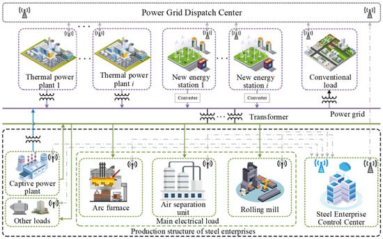
As a typical high energy industrial user, the production load structure of iron and steel enterprises is shown in Figure 1. From the perspective of system, conventional thermal power units and new energy power sources jointly undertake the basic power supply task and maintain the power balance of the system, which together constitute the main body of power supply. From the perspective of users, iron and steel enterprises are equivalent to a comprehensive energy unit, which is composed of self-owned power plants and main production loads, and participate in system scheduling through a unified interface [16]. Different types of production loads show great differences in operation characteristics and regulation time scales. One type of load is constrained by process continuity and safety requirements, with strong operation rigidity and relatively limited regulation space. The other type of load has a certain regulation flexibility under the premise of meeting the production process constraints and can be excavated as a potential resource of system flexibility to participate in the collaborative optimal dispatch of power system. In order to support the modeling of production load in iron and steel enterprises and the coupling analysis of self-provided power plants, the composition structure and adjustable characteristics of power load in iron and steel enterprises should be described in a unified way.

Figure 1. Schematic diagram of the steel production load structure.

From the perspective of production process, the power load of iron and steel enterprises mainly includes smelting main process load, production auxiliary load and post-treatment processing load. Among them, the power level of smelting equipment such as EAF changes periodically with the furnace operation, which is the main source of electricity for enterprises. Auxiliary loads such as the ASU are usually coupled with the medium storage link and have a certain cross-time regulation ability under the conditions of safe operation. Processing loads such as steel rolling lines can be started and stopped when the production plan and inventory permit, showing interruptible characteristics [17,18]. Comparatively speaking, the auxiliary facilities in the plant and some continuous process loads have high requirements for production safety and continuity, and the adjustment space is limited [19].

In this study, the total power load of iron and steel enterprises is divided into basic load and adjustable load. Among them, the base load is the rigid energy load in the dispatching process, which has the characteristic of being non-adjustable. The adjustable load is mainly composed of the EAF, ASU and steel rolling line [20], which is a nuclear psychoactive resource for steel enterprises to participate in system peak shaving and new energy consumption. On this basis, by analyzing the characteristics of different loads in terms of regulation mode and process constraints, the adjustable load is subdivided into continuous adjustable load, transferable load and interruptible load, laying the foundation for subsequent differential modeling [21].

2.2. Flexibility Analysis and Modeling of Typical Steel Production Processes

2.2.1. Operational Characteristics and Flexibility Modeling of EAF

As the primary equipment in the steelmaking process, EAFs account for approximately 40% of the total energy consumption of steel enterprises and therefore represent a typical energy-intensive load. The production process of EAFs exhibits pronounced flexibility characteristics [22,23]

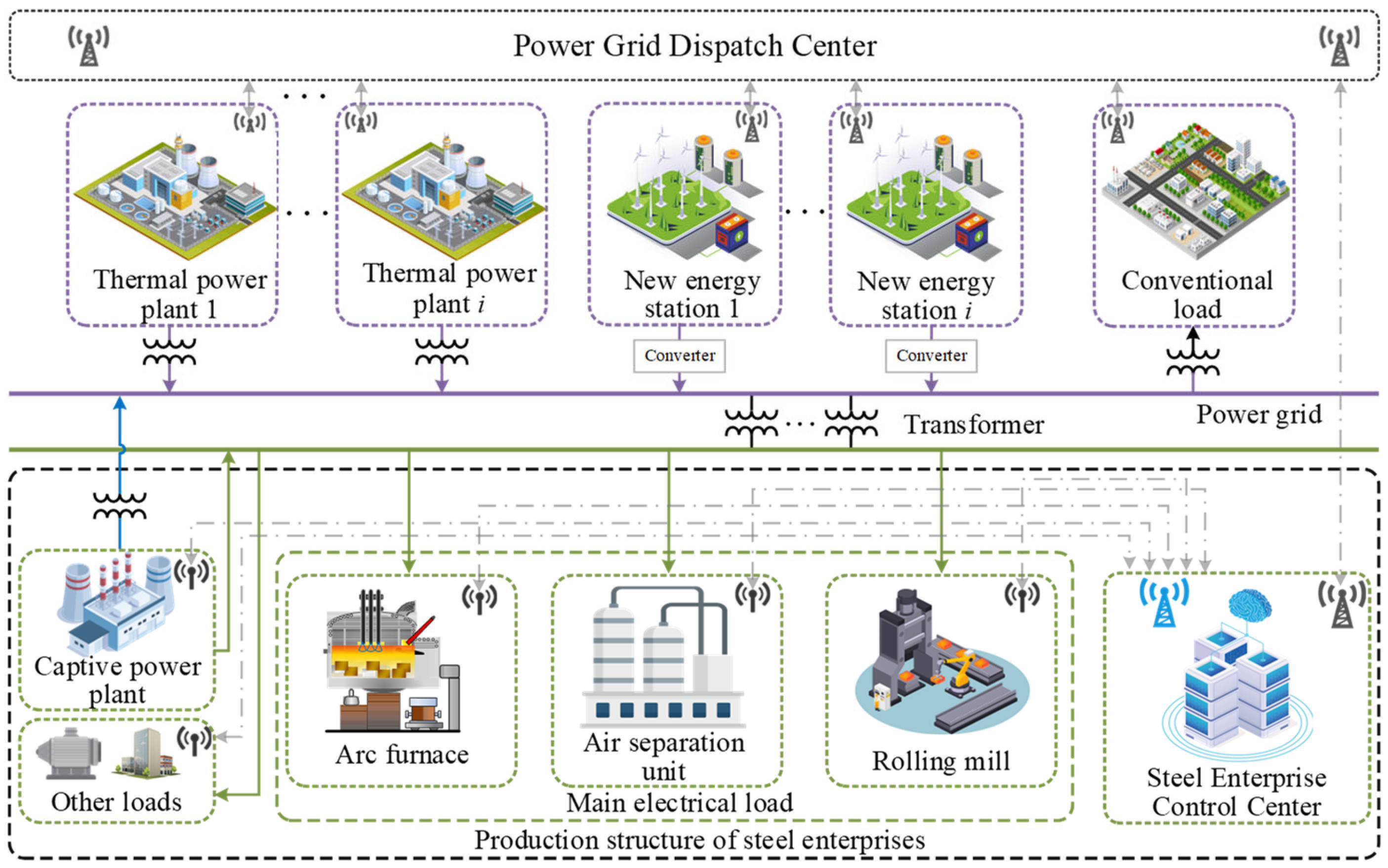
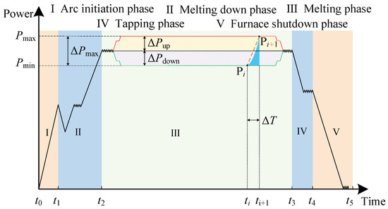
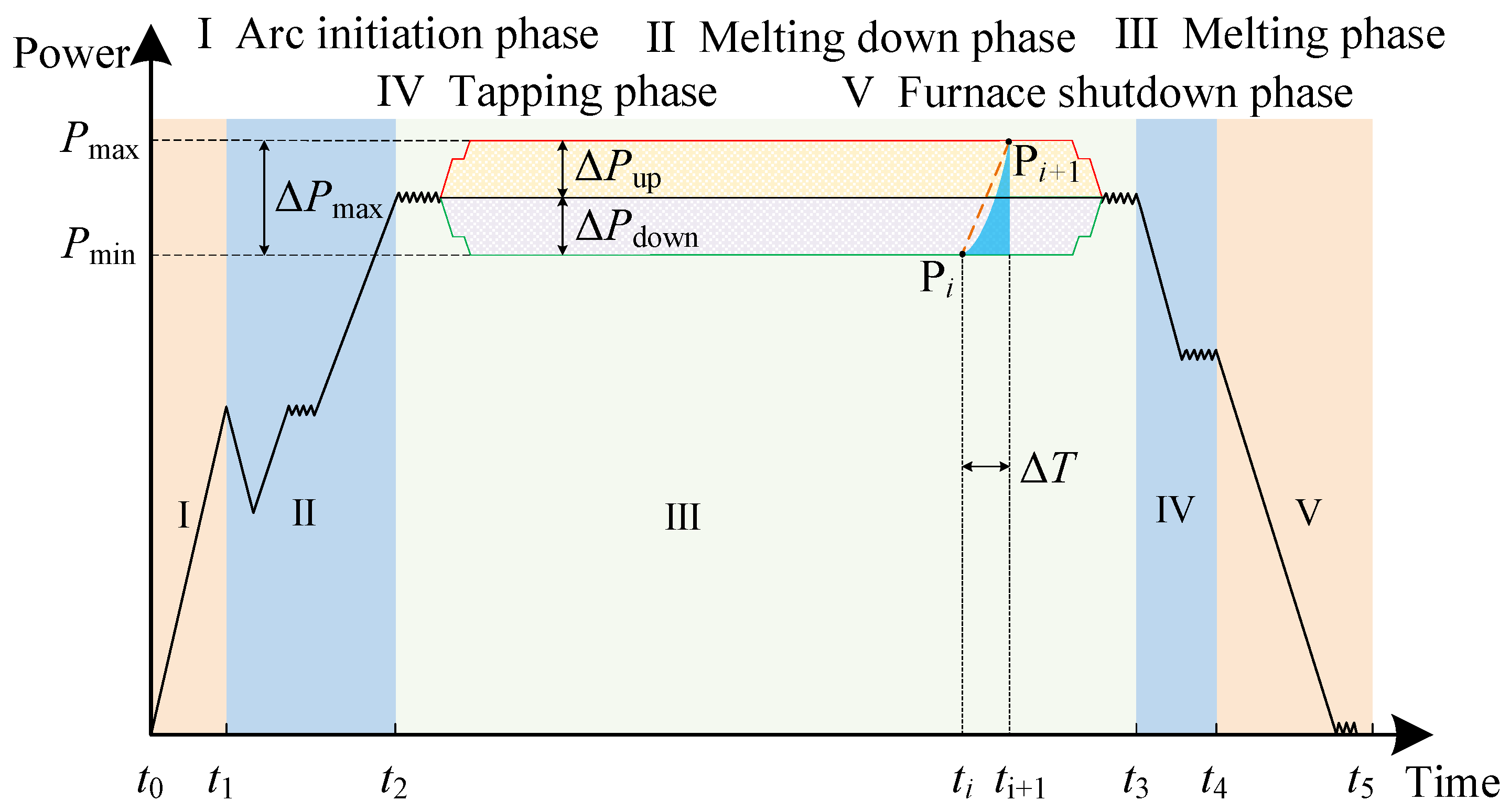
Figure 2 illustrates the schematic power variation over an EAF smelting cycle. The entire smelting cycle consists of five stages: arc ignition, bore-in, melting, furnace shutdown, and tapping. Among these stages, the melting period accounts for approximately 70% of the total smelting cycle. Accordingly, when optimizing the enterprise production schedule, power regulation of the EAF is mainly performed during the arc ignition and melting stages [24,25]. With respect to the EAF power regulation mechanism, this paper adopts transformer tap-changing as the means of power adjustment, which is more consistent with practical EAF operating conditions.

Figure 2. Typical power profile of an EAF during a smelting cycle.

Therefore, the power constraints of the EAF can be expressed as

$$\left\{\begin{array}{l}{P}_{i,t}^{\mathrm{E}}=x_{i,t}\left[(1+c{\beta }_{i,t})P_{i,t}^{\mathrm{E},0}\right]\\ {\beta }_{i,t}\in \left\{-\mathrm{R}\cdots -1,0,1\cdots ,R\right\}\end{array}\right.$$

(1)

where P^E_i,t denotes planned operating power of the ith EAF at time t; x_i,t denotes operation status identification of the ith EAF at time t, where x = 1 indicates the EAF is in operation; and x = 0 indicates EAF shutdown state. c is a constant term that corresponds to the initial rated power percentage; β_i,t designates actual gear of transformer tap of the ith EAF at time t. P^E,0_i,t is the planned power for EAF i at time t; R denotes the highest gear of transformer tap of the ith EAF.

Due to the significant impact of EAF power variations on the power grid, in practical operation the transformer tap position is not allowed to change by skipping intermediate steps. In addition, constraints are imposed on the number of consecutive tap adjustments of the EAF:

$$\left|{\beta }_{i,t}-{\beta }_{i,t-1}\right|\le 1$$

(2)

$$0\le \left[{\displaystyle \sum _{t=2}^T\left(\left|S_1^t-S_1^{t-1}\right|+\left|S_2^t-S_2^{t-1}\right|\right)}\right]/2\le M$$

(3)

where T denotes the total number of time intervals within the dispatch period. S^t₁ and S^t₂ are binary state variables representing the upward and downward power regulation states of the EAF at time interval t, respectively, with S^t₁, S^t₂ ∈{0,1}. S^t₁ = 1 indicates that the EAF is in upward regulation state at time t, while S^t₂ = 1 indicates downward regulation state. S^t₁ + S^t₂ ≤ 1 ensures that the EAF cannot perform upward and downward regulation simultaneously. M denotes the maximum allowable number of regulation actions within the dispatch period.

During the operation of the EAF, to ensure production efficiency and product quality, constraints are imposed on the maximum and minimum smelting durations of each heat. The time constraints for a single smelting heat are given by

$${\displaystyle \sum _{t=\epsilon }^{\epsilon +T_{\max }}{x}_{i,t}}\le T_{\max }\epsilon \in \left[1,T-T_{\max }\right]$$

(4)

$$x_{i,t}-x_{i,t-1}\le x_{i,\tau }\tau \in \left[t,\min \left(T,t+T_{\min }-1\right)\right]$$

(5)

where x_i,t∈{0,1} is the binary state of EAF i at time t (1 = operational, 0 = idle), T is the total number of time periods in the scheduling horizon, and T_max, T_min denote the maximum and minimum duration per heat cycle, respectively. The index τ represents time intervals within the range [t, min(T,t + T_min − 1)], ensuring that once the EAF is started, it must remain in operation for at least T_min consecutive intervals. This constraint ensures that if EAF i is started at time t (x_i,t − x_i,t−1 = 1), it must remain operational for at least T_min consecutive periods to complete the smelting process

To ensure that product output remains unchanged before and after the participation of the steel enterprise in system dispatch, a constraint is imposed on the minimum electrical energy required to meet the production output, as expressed by the following equation:

$${\displaystyle \sum _{t=1}^T\left(P_{i,\mathrm{on}}^{\mathrm{E}}+\Delta P_{i,t}^{\mathrm{E}}\right)}\Delta t\ge Q_{\mathrm{pre}}$$

(6)

where ΔP^E_i,t denotes the adjustable power of EAF i during time interval t; Δt denotes the duration of a dispatch period; Q_pre denotes the minimum electricity required for production output within a dispatch period.

2.2.2. Operational Characteristics and Flexibility Modeling of ASU

As an important auxiliary facility in the steelmaking process, the ASU mainly supplies gases such as oxygen and nitrogen required for production. Its electricity consumption accounts for approximately 15% of the total electricity consumption of a steel enterprise. Each type of gas is equipped with a corresponding gas holder, and under the premise of ensuring safe gas storage, the ASU exhibits shiftable flexibility characteristics. The corresponding constraints are formulated as follows [26,27]:

The gas output of the ASU is proportional to its electricity consumption:

$$P_{j,t}^{\mathrm{gas}}=p_j{V}_{j,t}$$

(7)

where P^gas_j,t denotes the power consumed for producing gas j during time interval t; p_j denotes the specific power consumption per unit volume of gas j; V_j,t denotes the volume of gas j produced in time interval t.

To account for gas storage safety and the production capacity of the ASU, the constraints on the variation of gas volume in the gas holder are formulated as follows:

$$V_{j,\min }\le V_{j,t}\le V_{j,\max }$$

(8)

$$\left|V_{j,t}-V_{j,t-1}\right|\le \Delta V$$

(9)

where V_j,max, V_j,min denote the upper and lower capacity limits of the gas holder storing gas j; V_j,t denotes the volume of gas j at time interval t; ΔV denotes the maximum allowable volume change between adjacent time intervals.

2.2.3. Operational Characteristics Analysis and Modeling of Rolling Mill Loads

Rolling is an essential stage in steel production, including different processes such as hot rolling and cold rolling. Hot rolling shapes heated steel billets through rolling mills, while cold rolling further processes steel products at ambient temperature [28,29]. From a technical perspective, when sufficient steel inventory is available, rolling production lines can be shut down with advance notice. Therefore, rolling mill loads can be regarded as interruptible loads for dispatch purposes.

The corresponding modeling based on its interruptible characteristics is formulated as follows:

$$P_t^{\mathrm{roll}}=d_t{P}_t^{\mathrm{roll},0}$$

(10)

$${\displaystyle \sum _{t=1}^T{d}_t\ge (T-T^{\mathrm{shut}})}$$

(11)

where P_t^roll denotes the actual power of the rolling load in period t; d_t denotes the start and stop variable of the rolling load in period t; d_t = 1 indicates that the rolling load is in operation; d_t = 0 means that the rolling load is at a stop state; P_t^roll,0 denotes the scheduled power of the rolling load at time t; T^shut denotes the number of interruption periods for the rolling load within the dispatch period t.

2.3. A Capacity Regulation Model Integrating the Energy Supply System and the Production Process

The energy supply system of a steel enterprise mainly consists of on-site power generation and electricity purchased from the grid. To investigate the flexible regulation capability of captive power generation resources, it is necessary to equivalently aggregate the generation side and the consumption side into an equivalent load, which responds to the external system as an integrated entity [30,31].

2.3.1. Output Constraints of the Captive Power Plan

Assume that the captive power plant of a steel enterprise consists of N generating units. A generation schedule is to be determined over T equal-length time periods. The corresponding power output constraints are formulated as follows:

Upper and Lower Output Limits of Captive Generating Units:

$$P_{n,\min }^{\mathrm{g}}\le P_{n,t}^{\mathrm{g}}\le P_{n,\max }^{\mathrm{g}}$$

(12)

where P^g_n,min, P^g_n,max denote the minimum and maximum output limits of the n-th captive generating unit respectively; P^g_n,t denotes the actual output of the n-th captive generating unit during time interval t.

Ramping Constraints of Captive Generating Units:

$$\left|P_{n,t}^{\mathrm{g}}-P_{n,t-1}^{\mathrm{g}}\right|\le \Delta P_{n,\mathrm{up}}^{\mathrm{g}}$$

(13)

where ΔP^g_n,t denotes the ramping rate of the n-th captive generating unit at time interval t.

Energy–Power Integral Constraint of Captive Generating Units:

$$Q_{n,t}^{\mathrm{g}}={\displaystyle {\int }_{\left(t-1\right)\Delta \mathrm{t}}^{t\Delta \mathrm{t}}{P}_{n,t}^{\mathrm{g}}}\mathrm{d}t$$

(14)

where Q^g_n,t denotes the energy output of the n-th captive generating unit during time interval t.

2.3.2. Coupling Model Between the Power Supply System and the Electricity Consumption System

The above modeling of the energy supply system and adjustable production processes is coupled through power balance constraints.

$${\displaystyle \sum _{n=1}^N{P}_{n,t}^{\mathrm{g}}}+k{P}_t^{\mathrm{net}}={\displaystyle \sum _{i=1}^I{P}_{i,t}^{\mathrm{E}}}+{\displaystyle \sum _{j=1}^J{P}_{j,t}^{\mathrm{gas}}+P_t^{\mathrm{roll}}}+P_t^{\mathrm{base}}$$

(15)

where N denotes the number of generating units in the CPP; P^net_t denotes the net interchange power between the steel enterprise and the grid at time t; k denotes the symbol of power purchase and sale of iron and steel enterprises. k = 1 means power purchase from abroad, k = −1 means power sale from abroad, and P_t^base denotes the basic load of iron and steel enterprises.

2.3.3. Adjustable Capacity Model Under the Coupling of the Power Supply System and Production Processes

The adjustable capacity consists of the adjustable capacity of captive generating units and that of production loads.

$$\begin{array}{ll}{P}_{adj,t}& ={\displaystyle \sum _{n=1}^N\left(P_{n,t}^{\mathrm{g},0}-P_{n,t}^{\mathrm{g}}\right)+}{\displaystyle \sum _{i=1}^I\left(P_{i,t}^{\mathrm{E}}-P_{i,t}^{\mathrm{E},0}\right)}\\ & +{\displaystyle \sum _{j=1}^J\left(P_{j,t}^{\mathrm{gas}}-P_{j,t}^{\mathrm{gas},0}\right)+P_t^{\mathrm{roll}}-}{P}_t^{\mathrm{roll},0}\end{array}$$

(16)

where P_adj,t denotes the adjustable power of the steel enterprise at time t; P^g,0_n,t denotes the pre-adjustment scheduled output of captive unit n during period t; P^E,0_i,t denotes the pre-adjustment planned power for EAF n at time t; P^gas,0_j,t denotes the pre-shift planned power for ASU j at time t; P^roll,0_t denotes the pre-interruption planned power for rolling load n at time t.

3. Day-Ahead and Intra-Day Scheduling Considering the Flexibility of Steel Enterprises

In order to ensure the economy and security of the new power system with a high proportion of renewable energy connected to the grid, scheduling decisions usually need to be made on multiple time scales. In this paper, the unified modeling and optimization analysis of the power system operation process with the participation of iron and steel enterprises are carried out by constructing a day-ahead and intra-day two-stage scheduling framework. In the day-ahead scheduling stage, based on the day-ahead wind power output prediction and conventional load prediction, the optimal solution of the system thermal power unit output and the equivalent port power of iron and steel enterprises is obtained, and the optimal day-ahead operation plan is obtained. In the intra-day stage, with the continuous update of the forecast information, considering the wind power forecast error, the iron and steel enterprises will be equipped with energy storage. Through the rapid response of energy storage, the day-ahead plan will be corrected in real time, so as to reduce the impact of the wind power forecast error on the system and the operation of the iron and steel enterprises [32].

3.1. Day-Ahead Scheduling Model

The day-ahead dispatching phase takes 24 h as a dispatching cycle, divides the dispatching time into 96 periods, and optimizes the system operation scheme based on the day-ahead wind power output prediction and conventional load prediction. The main objective of this stage is to determine the output plan of thermal power units, the consumption level of wind power and the power purchased and sold by iron and steel enterprises, so as to provide a benchmark scheme for subsequent day dispatching.

3.1.1. Objective Function

The day-ahead scheduling model aims to minimize the total operating cost of the system, taking into account the operating cost of thermal power units, the penalty cost of wind power curtailment, and the electricity consumption cost of the steel enterprise. The objective function can be expressed as

$$\min F_{DA}=C_{\mathrm{f}}+C_{\mathrm{w}}+C_{\mathrm{s}}$$

(17)

Operating Cost of Thermal Power Units:

$$C_{\mathrm{f}}={\displaystyle \sum _{t=1}^T{\displaystyle \sum _{u=1}^U\left[a_u{\left(P_{u,t}^{\mathrm{G}}\right)}^2+b_u{P}_{u,t}^{\mathrm{G}}+c_u\right]}}$$

(18)

where a_n, b_n, and c_n are the fuel (coal consumption) cost coefficients of captive generating unit n.

Wind Power Curtailment Penalty Cost:

$$C_{\mathrm{WC}}={\displaystyle \sum _{t=1}^T{K}_q\left(P_{w,t}^{\mathrm{pre}}-P_{w,t}\right)}$$

(19)

where P_w,t denotes the actual accommodated wind power at time period t.

Operating Cost of the Steel Enterprise:

$$C_{\mathrm{s}}={\displaystyle \sum _{t=1}^T{\displaystyle \sum _{n=1}^N\left[a_n{\left(P_{n,t}^{\mathrm{g}}\right)}^2+b_n{P}_{n,t}^{\mathrm{g}}+c_n\right]}}+B{P}_t^{\mathrm{buy}}-C{P}_t^{\mathrm{sell}}$$

(20)

where P_t^buy and P_t^sell denote the electricity purchasing power and selling power of the steel enterprise at time period t, respectively; B is the electricity purchasing cost coefficient of the steel enterprise; and C is the revenue coefficient associated with electricity sales.

3.1.2. Constraints

System Power Balance Constraint:

$${\displaystyle \sum _{u=1}^U{P}_{u,t}^{\mathrm{G}}}+P_{w,t}=k{P}_t^{\mathrm{net}}+P_t^{\mathrm{L}}$$

(21)

where P_t^L denotes the forecasted conventional load power at time period t.

Day-Ahead Wind Power Output Constraints:

$$0\le P_{w,t}\le P_{w,t}^{\mathrm{pre}}$$

(22)

where P_w,t denotes the actual day-ahead wind power output and P^pre_w,t denotes the forecasted day-ahead wind power output at time period t.

Upper and Lower Output Limits of Thermal Power Units:

$$P_{\min }^{\mathrm{G}}\le P_{u,t}^{\mathrm{G}}\le P_{\max }^{\mathrm{G}}$$

(23)

where P^G_min and P^G_max denote the lower and upper output limits of the thermal power units, respectively.

Ramping Constraints of Thermal Power Units:

$$\left|P_{u,t}^{\mathrm{G}}-P_{u,t-1}^{\mathrm{G}}\right|\le \Delta P_{u,\mathrm{up}}^{\mathrm{G}}$$

(24)

where ΔP^G_up denotes the maximum ramp-up rate of a thermal power unit between adjacent time periods.

Transmission Line Capacity Constraints:

$$\left|P_t^{\mathrm{T}}\right|\le P_{\max }^{\mathrm{T}}$$

(25)

where P_t^T denotes the active power transmitted by the transmission line at time period t, and P^T_max represents the maximum allowable transmission power of the line.

3.2. Intra-Day Scheduling Model

Unlike day-ahead scheduling, which focuses on the overall economy of the system, day-ahead scheduling mainly focuses on the ability of the system to cope with the prediction error and the stability of operation in a short time scale. Considering that the production load of iron and steel enterprises is affected by process constraints, and it is difficult to adjust frequently within the intra-day scale, this paper introduces the iron and steel enterprise side energy storage system in the intra-day scheduling stage, and uses its rapid response characteristics to undertake the main task of power balance adjustment, so as to stabilize the power fluctuation in load operation and reduce the impact on the power grid [33].

3.2.1. Objective Function

In the day scheduling stage, based on the day-ahead scheduling results and further considering the impact of wind power prediction error, the total operating cost of the system is minimized by coordinating and adjusting the output of thermal power units, the production plan of iron and steel enterprises and the charging and discharging power of energy storage system. The objective function can be expressed as

$$\min F_{\mathrm{ID}}={\displaystyle \sum _t^T\left(\begin{array}{l}{C}_t^{\mathrm{TH}}+C_t^{\mathrm{WC}}+C_t^{\mathrm{EAF}}+C_{\mathrm{t}}^{\mathrm{OXY}}\\ \begin{array}{l}\hfill \end{array} +C_t^{\mathrm{ROLL}}+C_t^{\mathrm{ZB}}+C_t^{\mathrm{ESS}}\end{array}\right)}$$

(26)

Intra-Day Operating Cost of Thermal Power Units:

$$C_t^{\mathrm{TH}}={\displaystyle \sum _{t=1}^T{\displaystyle \sum _{u=1}^U\left[a_u{\left(P_{u,t}^{\mathrm{G}}\right)}^2+b_u{P}_{u,t}^{\mathrm{G}}+c_u\right]}}$$

(27)

where U denotes the total number of thermal power units in the system; a_u, b_u, and c_u are the fuel (coal consumption) cost coefficients of thermal power unit u; and P^G_u,t represents the actual output power of thermal power unit u at time period t.

Intra-Day Wind Power Curtailment Penalty Cost:

$${\displaystyle \sum _t^T{C}_t^{\mathrm{WC}}}={\displaystyle \sum _{t=1}^T{K}_q\left(P_{w,t}^{\mathrm{pre},\mathrm{id}}-P_{w,t}^{\mathrm{id}}\right)}$$

(28)

where K_q denotes the wind power curtailment penalty coefficient; P^pre,id_w,t represents the intra-day forecasted wind power at time period t; and P^id_w,t denotes the actual accommodated wind power in the intra-day stage at time period t.

Operating Cost of the Captive Power Plant:

$${\displaystyle \sum _t^T{C}_t^{\mathrm{ZB}}}={\displaystyle \sum _{t=1}^T{\displaystyle \sum _{n=1}^N\left[a_n{\left(P_{n,t}^{\mathrm{g}}\right)}^2+b_n{P}_{n,t}^{\mathrm{g}}+c_n\right]}}$$

(29)

where a_n, b_n, and c_n are the fuel (coal consumption) cost coefficients of captive generating unit n.

Maintenance Cost of Electrochemical Energy Storage:

$${\displaystyle \sum _t^T{C}_t^{\mathrm{ESS}}}={\displaystyle \sum _{t=1}^T{K}_{\mathrm{es}}(P_t^{\mathrm{ch}}+P_t^{\mathrm{dis}})}$$

(30)

where K_es denotes the unit charging and discharging cost of the electrochemical energy storage per unit time. It should be noted that this paper adopts an approximate model in which the energy storage degradation cost is linear with the energy throughput, so as to maintain the linear structure of the dispatch model. More sophisticated nonlinear lifetime modeling will be further investigated in future work; P_t^ch and P_t^dis denote the charging power and discharging power of the electrochemical energy storage at time period t, respectively.

Power Regulation Cost of EAFs:

$${\displaystyle \sum _t^T{C}_t^{\mathrm{EAF}}}={\displaystyle \sum _t^T\left(s_1{P}_{\mathrm{up},t}^{\mathrm{EAF}}+s_2{P}_{\mathrm{down},t}^{\mathrm{EAF}}\right)}$$

(31)

where s₁ and s₂ denote the cost coefficients for upward and downward power regulation of the EAF, respectively, and P^EAF_up,t and P^EAF_down,t represent the amounts of upward and downward power adjustments of the EAF at time period t, respectively.

Regulation Cost of ASUs:

$${\displaystyle \sum _t^T{C}_t^{\mathrm{OXY}}}={\displaystyle \sum _t^{T}s\Delta P_t^{\mathrm{OXY}}}$$

(32)

where s denotes the regulation cost coefficient of the ASU, and ΔP_t^OXY represents the power adjustment of the ASU at time period t.

Interruption Cost of Rolling Mill Loads:

$${\displaystyle \sum _t^T{C}_t^{\mathrm{ROLL}}}={\displaystyle \sum _t^T{\mathrm{c}}_1{x}_t}$$

(33)

where x_t denotes the start-up/shut-down binary variable of the rolling mill at time period t, and c₁ represents the cost associated with a single start-up or shut-down of the rolling mill.

3.2.2. Constraints

System Power Balance Constraint

$${\displaystyle \sum _{u=1}^U{P}_{u,t}^{\mathrm{G}}}+P_{w,t}^{\mathrm{pre},\mathrm{id}}=P_t^{\mathrm{net}}+P_t^{\mathrm{ch}}-P_t^{\mathrm{dis}}+P_t^{\mathrm{L}}$$

(34)

Charging and Discharging Constraints of Electrochemical Energy Storage:

$$\left\{\begin{array}{l}\begin{array}{cc}& \end{array} 0\le P_t^{\mathrm{ch}}\le P_{\mathrm{ch}}^{\max } u_t^{\mathrm{ch}}\\ \begin{array}{cc}& \end{array} 0\le P_t^{\mathrm{dis}}\le P_{\mathrm{dis}}^{\max }{u}_t^{\mathrm{dis}}\\ u_t^{\mathrm{ch}}+u_t^{\mathrm{dis}}\le 1,u_t^{\mathrm{ch}},u_t^{\mathrm{dis}}\in \{0,1\}\end{array}\right.$$

(35)

where P^max_ch and P^max_dis denote the upper limit of the charging and discharging power of the battery; u_t^ch and u_t^dis denote the charging and discharging states of the energy storage system at time period t, respectively.

State-of-Charge (SOC) Constraints of Electrochemical Energy Storage:

$$\left\{\begin{array}{c}{E}_1=E_0+\Delta t\left({\eta }_{\mathrm{ch}}{P}_1^{\mathrm{ch}}-{\displaystyle \frac{1}{{\eta }_{\mathrm{dis}}}}{P}_1^{\mathrm{dis}}\right)\\ E_t=E_{t-1}+\Delta t\left({\eta }_{\mathrm{ch}}{P}_t^{\mathrm{ch}}-{\displaystyle \frac{1}{{\eta }_{\mathrm{dis}}}}{P}_t^{\mathrm{dis}}\right)\\ \begin{array}{c}\\ E^{\min }\le E_t\le E^{\max }\end{array}\end{array}\right.$$

(36)

where E_t denotes the energy stored in the energy storage system at time period t; η_ch and η_dis represent the charging and discharging efficiencies of the energy storage system, respectively; and E^min and E^max denote the minimum and maximum energy limits of the energy storage system.

3.3. Solution Method

The proposed day-ahead and intra-day two-stage optimal scheduling model that considers the operational flexibility of steel production loads is essentially a mixed-integer linear programming (MILP) problem [34], whose standard form is given in Equations (37) and (38).

$$\left\{\begin{array}{l}\min F_1(x,y)\\ s.t.\hfill & g_i(x,y)=0\hfill & i=1,2,\cdots ,m\hfill \\ & h_j(x,y)\le 0\hfill & j=1,2,\cdots ,n\hfill \\ & x_{\min }\le x\le x_{\max },\hfill & y\in \left\{0,1\right\}\hfill \end{array}\right.$$

(37)

$$\left\{\begin{array}{l}{x}_{\theta }\in \min F_2(x,z)\\ s.t.\hfill & {\lambda }_i(x,z)=0\hfill & i=1,2,\cdots ,p\hfill \\ & {\beta }_j(x,z)\le 0\hfill & j=1,2,\cdots ,q\hfill \\ & x_{\min }\le x\le x_{\max },\hfill & z\in \left\{0,1\right\}\hfill \end{array}\right.$$

(38)

where F₁(x,y) denotes the objective function of the day-ahead optimization, and F₂(x,z) denotes the objective function of the intra-day optimization. Here, x represents the continuous decision variables, which in this paper include the outputs of thermal power units, wind farm output, EAF regulation plans, ASU dispatch plans, and rolling mill dispatch plans. The vector y denotes the integer variables in the day-ahead optimization, including the electricity purchasing/selling states of the steel enterprise, as well as the operating states of EAFs, ASU, and rolling mills. The vector z represents the integer variables in the intra-day optimization, which correspond to the charging and discharging states of the electrochemical energy storage system

The equality constraints g_i(x,y) = 0 and inequality constraints h_j(x,y) ≤ 0 represent the equality and inequality constraints of the day-ahead optimization, respectively. In this study, the equality constraint in the day-ahead stage is the system power balance constraint, while the inequality constraints include thermal power unit constraints, wind farm power constraints, EAF operating constraints, ASU operating constraints, and rolling mill operating constraints. Similarly, the equality constraints λ_i(x,z) = 0 and inequality constraints β_i(x,y) ≤ 0 denote the equality and inequality constraints of the intra-day optimization, respectively. In this paper, the equality constraint in the intra-day stage is also the system power balance constraint, while the inequality constraints mainly include electrochemical energy storage constraints.

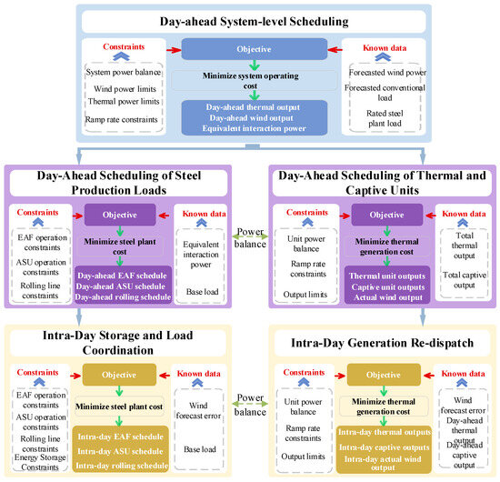
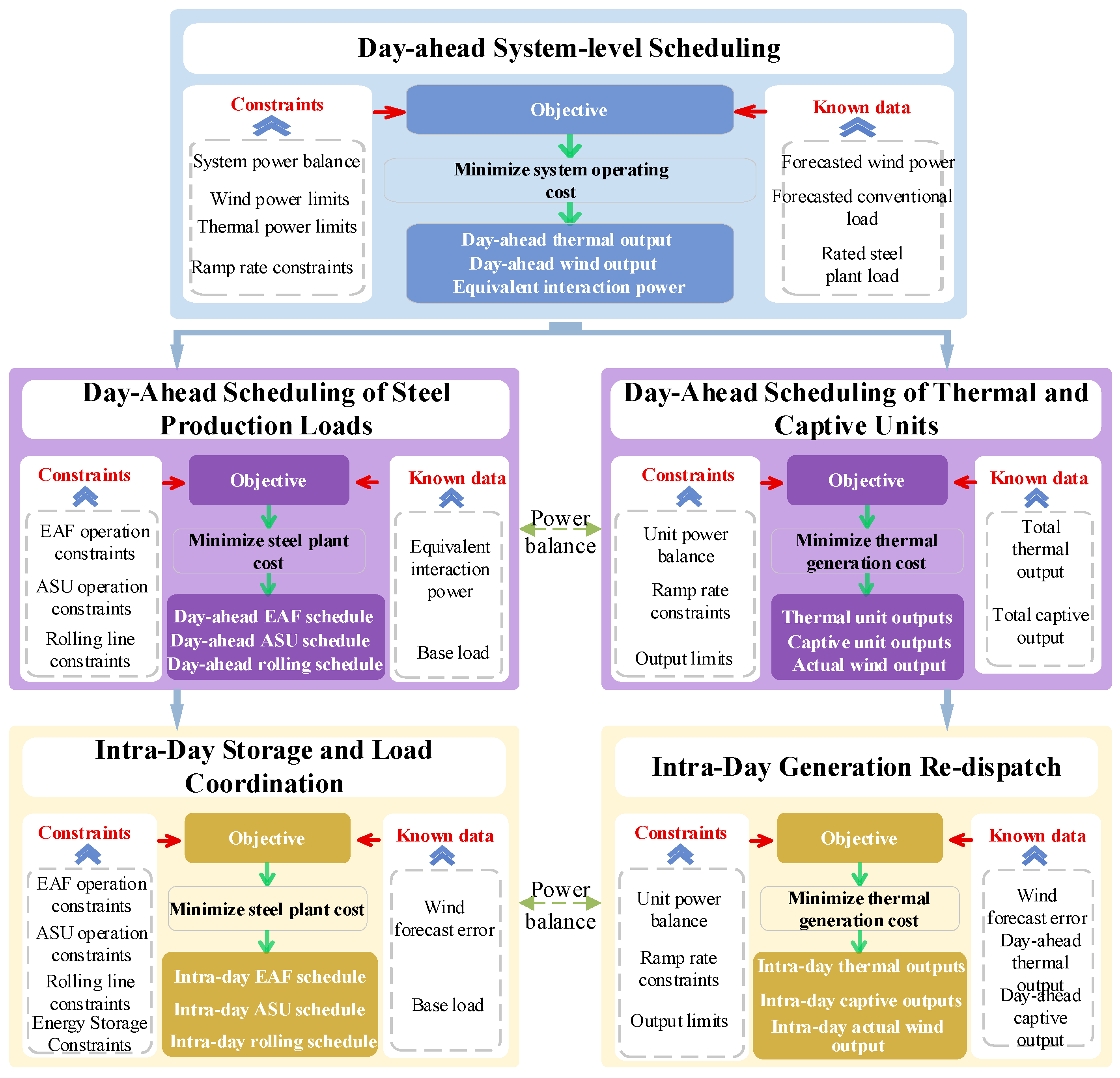
The term x_ϴ represents the results of the day-ahead optimization, including the day-ahead outputs of thermal power units and wind farms, as well as the production plans of various production loads within the steel enterprise. By incorporating the day-ahead scheduling results into the intra-day optimization, a more refined dispatch solution is obtained. Various methods are available for solving mixed-integer linear programming (MILP) problems; in practice, the CPLEX solver is commonly employed. The overall solution procedure is illustrated in Figure 3.

Figure 3. Day-ahead and intra-day coordinated scheduling framework.

4. Case Study

4.1. Case Study Parameter Settings

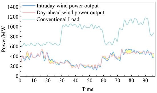
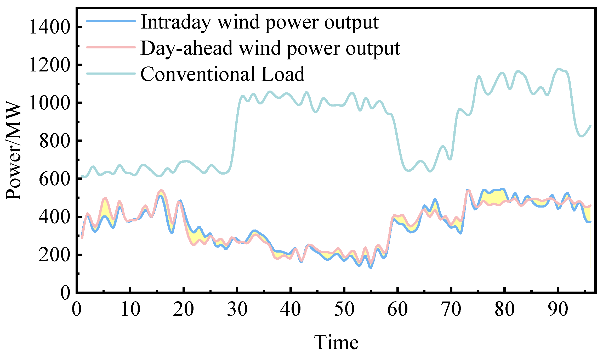
To verify the effectiveness and rationality of the proposed power system dispatch model with the participation of steel industrial loads, a regional test system is considered in this paper. The system consists of one thermal power plant, one large steel enterprise, one wind farm, and conventional loads. The thermal power plant includes five generating units with a total installed capacity of 1600 MW, and the detailed parameters are listed in Table 1. The wind farm has a total installed capacity of 600 MW, and its day-ahead and intra-day power output profiles are shown in Figure 4.

Table 1. Thermal power unit parameters.

Unit	Pmax/MW	Pmin/MW	a(¥/MW2·h)/b(¥/MW·h)/c(¥/h)	Ramp Rate/(MW/min)
1	300	90	0.0047/380/250	9
2	300	90	0.003/400/300	9
3	300	90	0.005/280/500	9
4	350	105	0.003/390/400	10
5	350	105	0.002/420/100	10

Figure 4. Day-ahead and intra-day wind power forecasts and conventional load profiles.

The steel enterprise is equipped with ten EAFs, one ASU, one rolling mill line, and a captive power plant. The parameters of the captive generating units are provided in Table 2. Each EAF has a rated operating power of 50 MW, and the EAF transformer includes nine discrete power regulation tap positions, with each tap corresponding to 5% of the rated power. The ASU consists of oxygen and nitrogen production units and is modeled as a shiftable load under the condition that the total daily gas output remains unchanged, with a maximum shifting capacity of 50 MW per 15 min. The rolling mill line is treated as an interruptible load with an operating power of 15 MW and can be interrupted up to five times per day. In addition, the steel enterprise is equipped with an energy storage system, whose detailed parameters are listed in Table 3.

Table 2. Captive power plant thermal unit parameters.

Unit	Pmax/MW	Pmin/MW	Ramp Rate/(MW/min)
1	100	60	2
2	100	60	2
3	100	60	2
4	200	120	4
5	200	120	4

Table 3. Parameters of the electrochemical energy storage system.

Emax/MW·h	Pch/Pdis/MW	ηch/ηdis	SOC0	SOCmax	SOCmin
100	30	0.95	0.5	0.9	0.2

To validate the proposed scheduling model, two scenarios are designed for comparative analysis to assess its effectiveness.

Scenario 1: The steel enterprise is not equipped with an energy storage system, and the system mainly relies on industrial loads to participate in intra-day power balancing.

Scenario 2: An energy storage system is introduced within the steel enterprise, and the energy storage is prioritized to undertake power regulation tasks in the intra-day stage caused by wind power forecast errors.

4.2. Analysis of Case Study Results

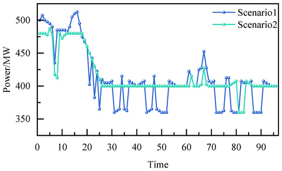
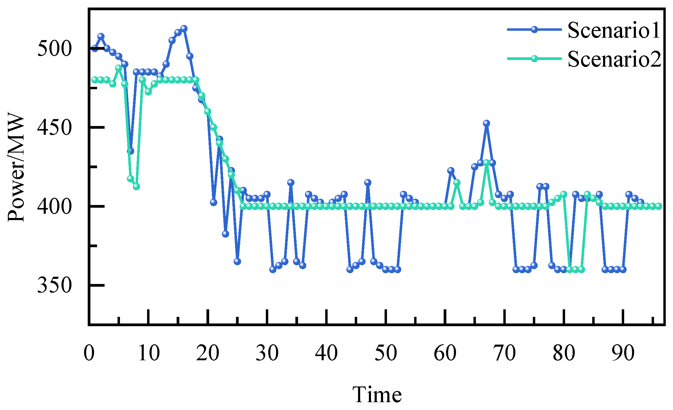
Figure 5 shows the operating power results of the EAF during the intra-day phase under two scheduling scenarios, where scenario 1 is the result of the energy storage device not participating in the scheduling, and scenario 2 is the result of the energy storage device participating in the scheduling. After analyzing the power curve, we found that there was not much difference in the average operating power of the EAF between the two scenarios. The average power of scenario 1 and scenario 2 were 412.29 MW and 416.04 MW, respectively. This indicates that after energy storage participated in scheduling, the overall operating level of the EAF did not change significantly, and the established production plan was effectively maintained. The introduction of energy storage did not achieve system balance by reducing production load.

Figure 5. EAF power profiles under two scenarios.

However, we can see from the graph that there are significant differences in power fluctuations between the two scenarios. In scenario 1, the operating power of the EAF fluctuates greatly, with a maximum operating power of 512.5 MW and a minimum operating power of 360 MW. The difference between the maximum and minimum power reaches 152.5 MW. At the same time, in order to effectively quantify the load fluctuation situation, this study uses the power standard deviation to quantify the fluctuation situation of each load. The power standard deviation corresponding to the EAF in scenario 1 is 45.16 MW, indicating the absence of energy storage configuration. In scenario 2, the maximum operating power of the EAF is 487.5 MW, the minimum operating power is 360 MW, and the difference between the maximum and minimum power is 127.5 MW. The corresponding power standard deviation of the EAF in scenario 2 is 31.80 MW. The above results indicate that in the absence of energy storage, the EAF frequently participates in power regulation during the daily scheduling phase. In contrast, after introducing an energy storage system in scenario 2, the operating power of the EAF significantly tended to flatten out, with power levels mostly concentrated around 400 MW and only adjusted during periods such as 62, 67, 81, 82, and 83. The power standard deviation decreased by 29.6% compared to scenario 1, indicating that the stability of the operating power of the EAF in scenario 2 has been effectively improved. In summary, without changing the overall power consumption scale of the EAF, if the energy storage system can significantly suppress the daily power fluctuations of the EAF and improve the stability of load operation. This is not only beneficial for ensuring the safe and stable operation of EAF equipment, but also to some extent reduces the impact of load fluctuations in steel enterprises on the operation of the power grid.

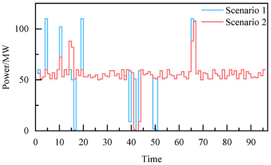
Figure 6 shows the operating power results of the ASU during the intra-day phase under different scenarios. The average power of the ASU remains consistent in both scenarios, at 55.15 MW. This is because, as a transferable load, the premise for the ASU to be transferable is to ensure its operational safety and production stability, that is, the amount transferred in during the entire scheduling cycle is equal to the amount transferred out, and the transfer amount needs to consider the capacity limit of the gas storage tank.

Figure 6. ASU power profiles under two scenarios.

However, there are significant differences in power fluctuations between the two scenarios. In scenario 1, the power fluctuation of the ASU is relatively frequent, with 10 extreme power points appearing, and the difference between the maximum and minimum operating powers reaching 110 MW. The standard deviation of the operating power of the ASU in scenario 1 is 17.31 MW. In contrast, after introducing an energy storage system in scenario 2, the power fluctuation of the ASU is effectively suppressed, with a difference of 107.22 MW between the maximum and minimum operating powers and seven extreme power points appearing, which is lower than in scenario 1. The standard deviation of the operating power is 12.46 MW, a decrease of 28.0% compared to scenario 1. The overall power operation curve is more stable.

Through the above analysis, we found that the energy storage system effectively mitigates load power fluctuations during the intra-day period, allowing for the power regulation behavior of the ASU to be more concentrated within a reasonable and sustainable operating range. Introducing an energy storage system in scenario 2 can significantly reduce the fluctuation in its daily operating power. This not only helps to ensure the safe and stable operation of the ASU, but also further reflects the buffering and protection role of energy storage in the two-stage scheduling framework for industrial production loads.

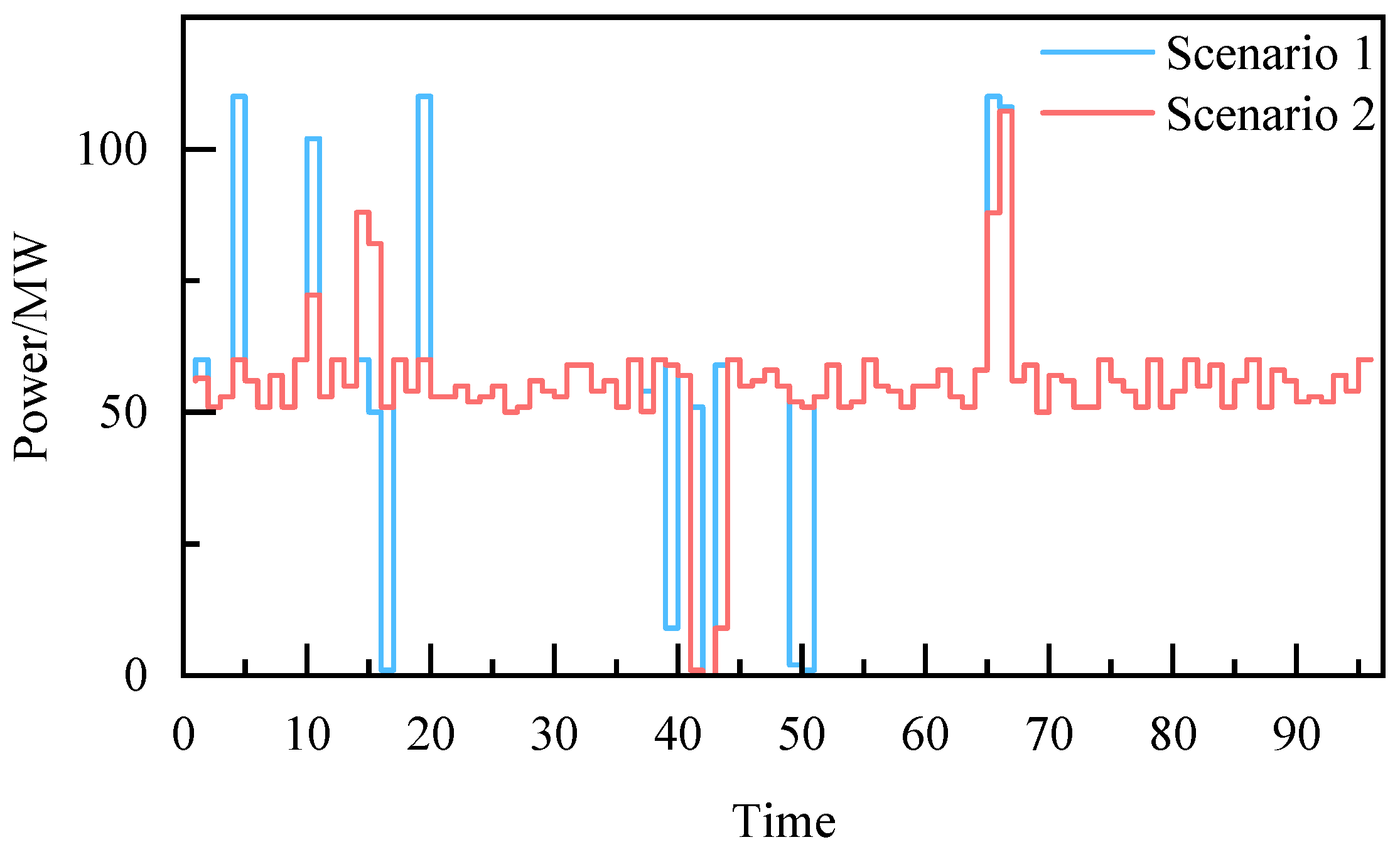
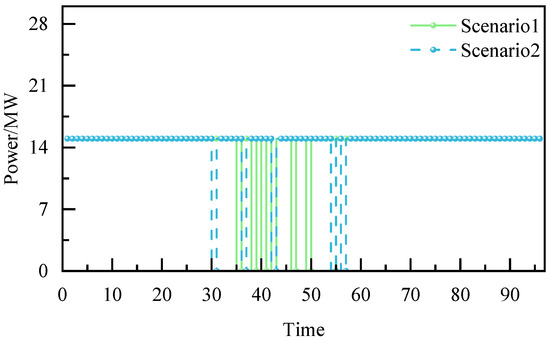
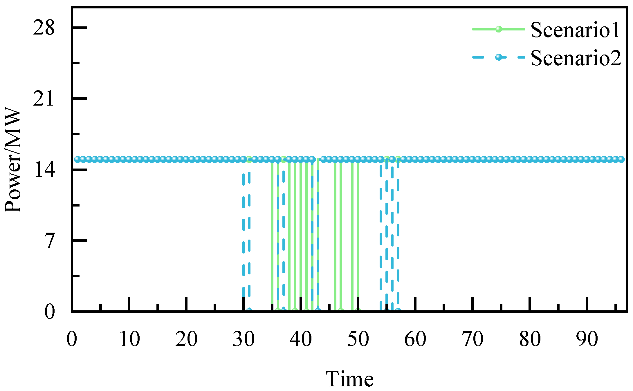
Figure 7 shows the operating power curves of the steel rolling line under different scenarios. From the curves in the figure, it can be seen that the operating power of the steel rolling line has interruptible load characteristics. In scenario 1, the steel rolling line experienced six interruptions during time periods 36, 39, 41, 43, 47, and 50. In scenario 2, after energy storage participates in scheduling, interruptions occur at time periods 31, 37, 43, 55, and 57, respectively. The interruption frequency of the steel rolling line has been reduced from six to five. By comparing the interruption time distribution of the steel rolling line in the two scenarios, we can see that the interruption distribution of the steel rolling line in scenario 1 is more concentrated, while the interruption distribution of the steel rolling line in scenario 2 is more scattered. This is because the energy storage system undertakes the main frequent power regulation task during the intra-day phase, reducing the system’s dependence on interruption regulation of the steel rolling line. When energy storage is not involved in scheduling, the steel rolling line is frequently used for power balance in the system, which affects the stability of production and operation to a certain extent. After energy storage participates in scheduling, the system prioritizes suppressing wind power prediction errors through energy storage charging and discharging levels and only interrupts the steel rolling line in a few cases. Scenario 2 ensures the continuity of steel production as a whole.

Figure 7. Rolling mill power profiles under two scenarios.

Table 4 compares the quantitative analysis results of the operational power stability of EAFs, ASUs, and steel rolling lines in different scenarios. From the table, although the average power consumption of major production units remains nearly unchanged, the proposed framework significantly reduces power fluctuation levels. The standard deviation of EAF and ASU power decreases by approximately 29.6% and 28%, respectively, indicating improved load smoothness and enhanced process stability. Therefore, the primary benefit of the proposed model lies in improving power quality and operational stability rather than merely reducing total energy consumption.

Table 4. Comparison of load operating stability under two scenarios.

Load Type	Metric	Scenario 1	Scenario 2	Change
EAF	Average Power/MW	412.29	416.04	Nearly Unchanged
	Power Fluctuation Range/MW	360–512.5	360–487.5	Range Converges
	Power Standard Deviation/MW	45.16	31.80	Reduced by 29.6%
ASU	Average Power/MW	55.15	55.15	Unchanged
	Power Fluctuation Range/MW	0–110	0–107.22	Range Converges
	Power Standard Deviation/MW	17.31	12.46	Reduced by 28%
Rolling Mill	Average Power/MW	15	15	Unchanged
	Number of Interruptions	6	5	Reduced
	Interruption Time Ratio/%	6.25	5.21	Reduced by 1.04%

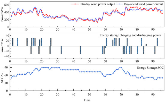
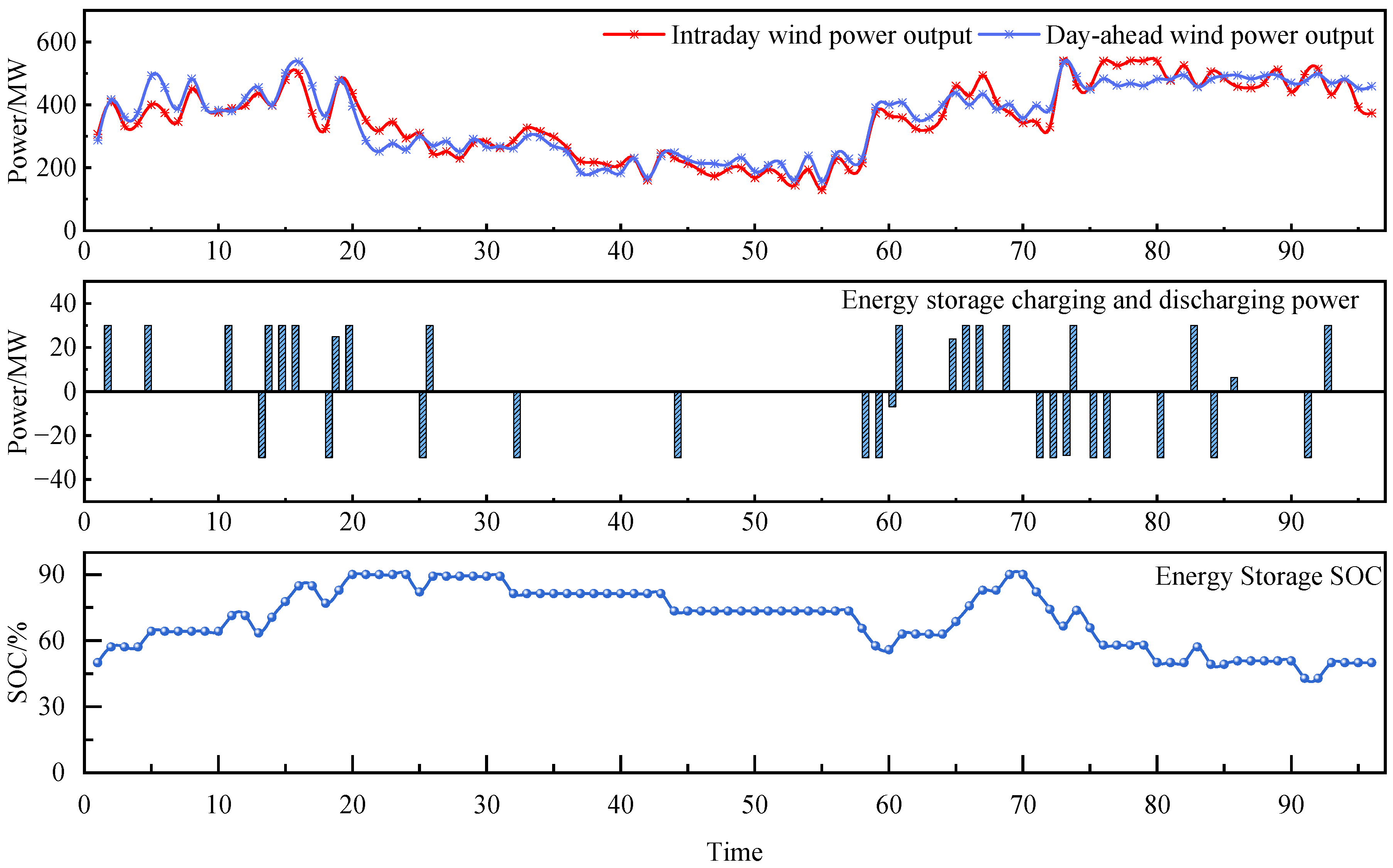
Figure 8 shows the wind power output and energy storage operation status during the previous day. It can be seen from the figure that due to prediction errors, there are significant deviations in wind power output during the day compared to the previous day at multiple time periods. The deviation is between −92.4 MW and +79.2 MW, and the time of significant deviation is mainly distributed between the periods of 2–25 and 59–81. That is to say, significant deviation mainly occurs at night, when the system load is in a low period. Therefore, the adjustment of steel load at this time increases sharply, causing significant pressure on the continuity and stability of steel production. The addition of energy storage devices has effectively alleviated these pressures. From the graph, it can be seen that energy storage charging and discharging are mainly concentrated in the periods of 2–26 and 58–84, while wind power is in a relatively large period corresponding to energy storage charging and discharging. Energy storage bears the majority of the regulation pressure for steel loads. Throughout the entire scheduling cycle, the cumulative charging capacity of energy storage is 505.17 MWh, and the cumulative discharging capacity is approximately 455.91 MWh. The participation of energy storage effectively weakens the direct transmission of wind power prediction bias to the load side and system side, making high-frequency regulation tasks prioritized by the energy storage system.

Figure 8. Day-ahead and intra-day wind power output and energy storage operating states.

In addition, during most of the time, the charging and discharging power of the energy storage system reached the rated power level, indicating that the energy storage system was fully utilized in the scheduling process and responded quickly to large deviations in wind power output. From the process of SOC state change, it can be seen that during periods of relatively high wind power output, the energy storage SOC gradually increases. When wind power output decreases, the SOC decreases accordingly, and its trend of change is consistent with the charging and discharging power. This result indicates that energy storage plays a good role in buffering wind power prediction errors during the intra-day scheduling phase.

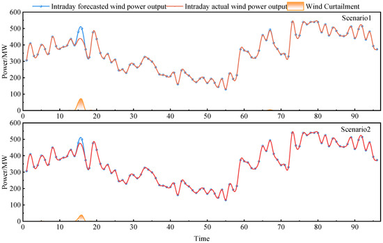
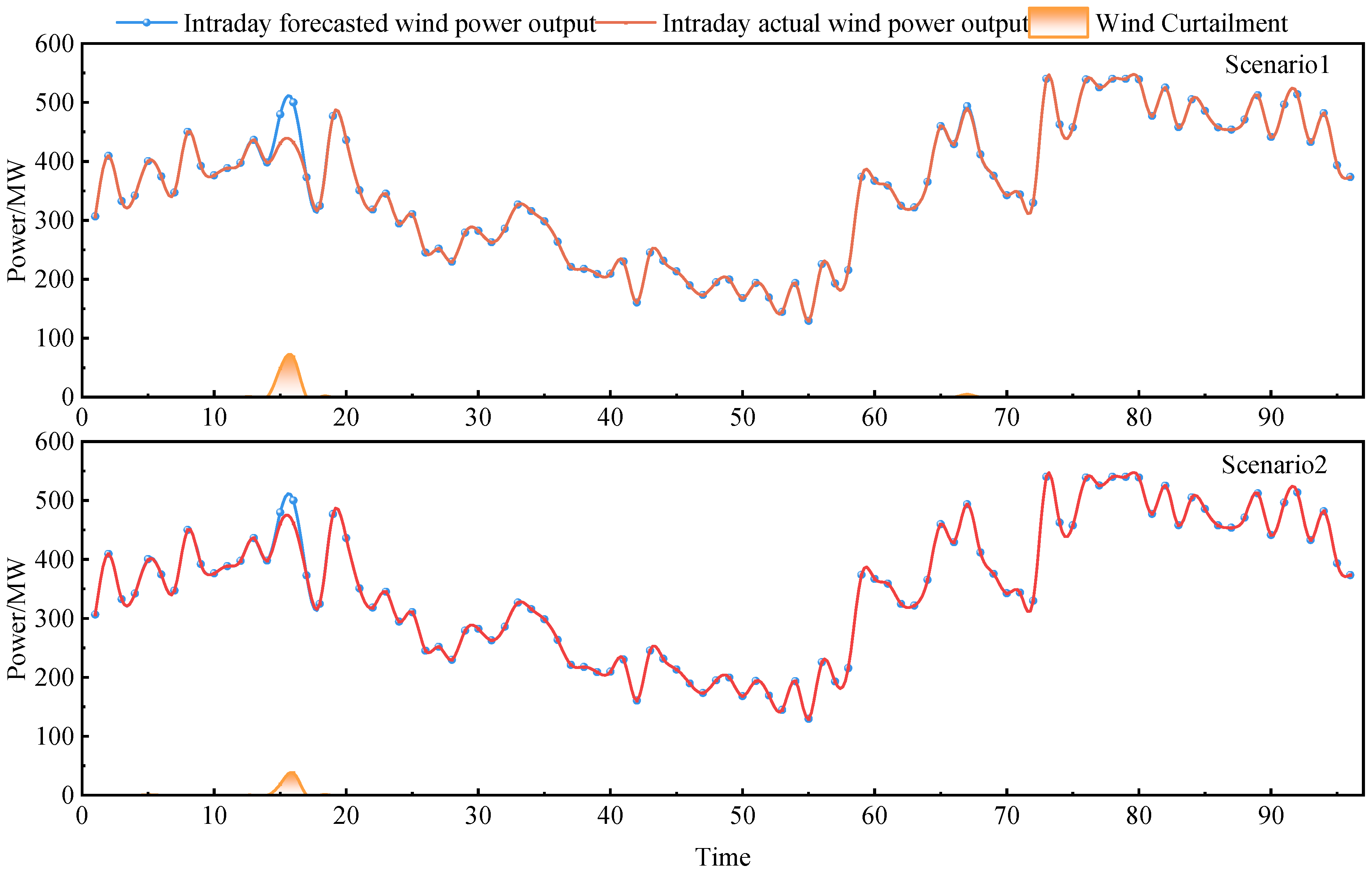
Based on the wind power output curves of the previous and current days in Figure 9, as well as the wind power curtailment results under two scheduling scenarios, it can be seen that the actual wind power output during the day was significantly higher than the previous plan in multiple time periods, with local peaks exceeding 500 MW and a maximum of about 540.17 MW. In the case of limited system regulation capacity, it became the direct source of wind power curtailment. In scenario 1, the phenomenon of wind power curtailment is mainly concentrated in a few periods when the wind power output significantly exceeds the system’s consumption capacity. Wind power curtailment only occurs in three periods, with corresponding curtailment powers of 48.90 MW, 68.10 MW, and 4.72 MW, respectively. The peak value of wind power curtailment reaches 68.10 MW, and the cumulative amount of wind power curtailment during the day is 30.43 MWh. In contrast, in scenario 2, there were significant changes in the scale and distribution characteristics of wind power curtailment, with corresponding curtailment powers of 1.08 MW, 0.14 MW, 18.90 MW, and 38.10 MW, respectively. The overall level of wind power curtailment was significantly reduced. Combining the energy storage charging and discharging curves, it can be found that when the wind power output is slightly higher than the system’s consumption capacity, the energy storage system preferentially enters the charging state to absorb surplus wind power, resulting in a high wind power utilization rate during most periods. Only when wind power remains at a high level and energy storage is constrained by power or SOC limits does the system generate a small amount of wind curtailment, and the wind power utilization curve shows a limited decrease. Therefore, compared to scenario 1, the decrease in wind power utilization rate in scenario 2 is significantly reduced.

Figure 9. Wind power curtailment results under different scenarios.

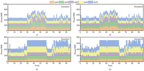
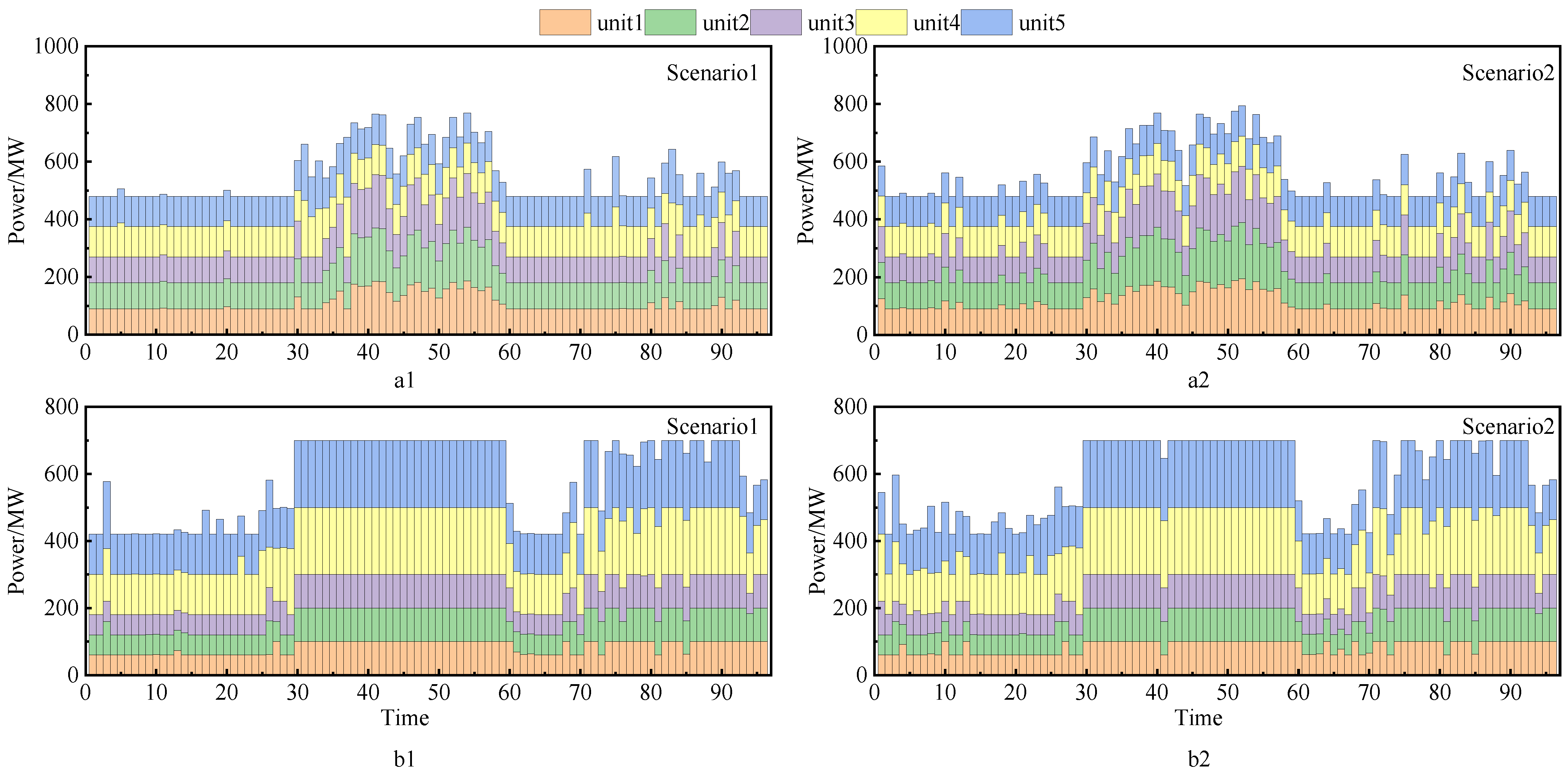
Figure 10 shows the output scheduling results of thermal power units. It can be seen that in scenario 1, the thermal power unit (a1) of the system undertakes frequent power regulation tasks during daily operation, and its output level shows obvious fluctuation characteristics with the change in system net load. Specifically, the average output of the thermal power units in this scenario is 548.88 MW, with a maximum output of 769.33 MW and a minimum output of 480.00 MW, corresponding to a standard deviation of 93.16 MW. In scenario 2, the average output of the thermal power units (a2) in the system is 556.60 MW, which is basically consistent with scenario 1. Among them, the maximum output of thermal power units is 793.69 MW, the minimum output is 480.00 MW, and the standard deviation of output is 97.01 MW. From the above analysis results, it can be seen that the average output of thermal power units in scenario 2 has increased compared to scenario 1, and the average output of thermal power units in scenario 1 is closer to the minimum output of the unit. If the wind power output increases at this time and the space for thermal power unit reduction is limited, it may cause more wind power curtailment, while the space for thermal power unit reduction in scenario 2 is higher than that in scenario 2, indicating that thermal power units with energy storage participation have better ability to cope with wind power fluctuations.

Figure 10. Output results of system thermal power units (a1,a2) and captive power plant units (b1,b2) under different scenarios.

From the output situation of the self-owned power plant units (b1, b2) of the steel enterprise, in scenario 1, the average output of the self-owned power plant units is 583.43 MW, with a maximum output of 700.00 MW and a minimum output of 420.00 MW, corresponding to a standard deviation of 124.12 MW. This indicates that in the absence of energy storage, the self-owned power plant units not only undertake basic power supply tasks but also need to frequently participate in system power regulation, resulting in relatively significant operational fluctuations. In contrast, in scenario 2, after energy storage participated in scheduling, the average output of the self-owned power plant units was 587.56 MW, with a standard deviation of 116.14 MW, a decrease of 6.4% compared to scenario 1. This indicates that energy storage has to some extent alleviated the regulation pressure of self-owned power plant units, eased their output fluctuations, and made their overall operating status more stable.

Table 5 compares the composition of system operating costs under the two scenarios. Scenario 1 represents the baseline dispatch scheme without energy storage participation, while scenario 2 corresponds to the scheme in which energy storage is deployed on the steel enterprise side and participates in coordinated day-ahead/intra-day scheduling. It can be observed that after the introduction of energy storage, the total system operating cost decreases from CNY 12,604,964.24 to CNY 12,562,496.73, representing an overall reduction of approximately 0.34%. It should be noted that the above cost reduction refers to operational cost savings during the scheduling horizon. The capital investment cost of energy storage is not included in the current model, and therefore the results reflect operational value rather than full life-cycle economic feasibility.

Table 5. Cost comparison across different scenarios.

Scenario	Total System Cost (¥)	TPU Cost (¥)	Wind Curtailment Penalty Cost (¥)	Steel Enterprise Electricity Cost (¥)
1	12,604,964.24	5,871,964.82	30,429.82	6,702,569.60
2	12,562,496.73	5,935,634.41	14,556.41	6,612,305.92

From the cost composition perspective, the operating cost of system thermal power units in scenario 2 increases slightly from CNY 5,871,964.82 to CNY 5,935,634.41. This is mainly because, after energy storage and steel enterprise-side loads participate in regulation, thermal power units are required to undertake more frequent power tracking and compensation tasks in certain periods, leading to increased ramping and regulation costs.

In contrast, the wind power curtailment penalty cost in scenario 2 decreases significantly, from CNY 30,429.82 to CNY 14,556.41, with a reduction of more than 50%. This demonstrates that energy storage plays an effective buffering role during periods with large wind power fluctuations and forecast deviations, thereby significantly enhancing the system’s wind power accommodation capability.

It can be seen from Table 6 and Table 7 that the mechanisms by which energy storage capacity and charging/discharging power affect system operation performance are significantly different.

Table 6. Sensitivity analysis of energy storage capacity.

Energy Storage Capacity	Wind Curtailment Rate (%)	EAF Load Volatility (%)
0	0.36	11.01
0.5Emax	0.17	8.47
Emax	0.17	7.68
1.5Emax	0.17	7.47
2Emax	0.17	7.41

Table 7. Sensitivity analysis of energy storage charging and discharging power.

Charging and Discharging Power (MW)	Wind Curtailment Rate (%)	EAF Load Volatility (%)
10	0.29	7.91
20	0.23	7.48
30	0.17	7.68
40	0.11	6.91
50	0.06	7.47

First, from the capacity sensitivity results, when the energy storage capacity increases from 0 to 0.5 E_max, the wind curtailment rate drops significantly from 0.36% to 0.17%. However, when the capacity further increases to E_max and above, the wind curtailment rate remains almost unchanged. This indicates that under the current charging power constraints, wind curtailment in the system is no longer limited by energy capacity but is mainly dominated by the instantaneous charging capability of energy storage. Meanwhile, although the EAF load volatility continues to decrease with the increase in capacity, the reduction range gradually diminishes, showing an obvious characteristic of diminishing marginal returns.

Further analysis from the power sensitivity shows that as the charging/discharging power increases from 10 MW to 50 MW, the wind curtailment rate decreases monotonically from 0.29% to 0.06% without an obvious plateau, which means that the renewable energy accommodation capability of the system is more sensitive to energy storage power. This result corroborates the capacity analysis and further demonstrates that the main bottleneck of the current system lies in power constraints rather than energy capacity. In terms of load smoothing effect, the EAF volatility reaches the lowest value (6.91%) when the power increases to 40 MW, after which the improvement slows down, indicating that there is also a reasonable range for power configuration.

Based on the two types of sensitivity results, it can be concluded that under the case conditions of this paper, energy storage capacity mainly affects the regulation duration capability, while charging/discharging power determines the instantaneous peak-shaving capability. The wind curtailment control of the system is more sensitive to power parameters, whereas load smoothing is jointly affected by both capacity and power with the characteristic of diminishing marginal returns. The benchmark configuration adopted in this paper (E_max, 30 MW) can already achieve significant wind curtailment suppression and fluctuation reduction effects, which is reasonable in balancing engineering practicability and regulation performance. Further increasing the power (e.g., to 40 MW) can achieve better smoothing effects, which belongs to a performance-enhanced configuration and can serve as a reference for subsequent engineering optimization.

5. Conclusions

In this paper, a two-stage day-ahead and intra-day coordination scheduling model considering the flexibility of steel production and industrial side energy storage is established. Through the analysis and verification of this model, the following conclusions can be drawn:

(1)

By taking energy storage as the main rapid response resource in the day stage, this paper effectively reduces the impact of wind power forecasting error on industrial load operation. The results of the case study show that the power fluctuation in steel production load is significantly reduced after energy storage participating in the scheduling: the standard deviation of EAF and ASU power is reduced by 29.6% and 28.0%, respectively, indicating that the operation stability and production continuity of steel production have been improved.

(2)

The coordinated dispatching strategy proposed in this paper effectively improves the wind power consumption of the system. Compared with the case without energy storage, the penalty cost of wind power curtailment in the system is reduced by more than 50%. Although the initial curtailment level is relatively low, the proposed strategy effectively reduces peak curtailment power and mitigates short-term renewable imbalance, demonstrating enhanced system flexibility under constrained operating conditions.

(3)

From the perspective of system operation, although the regulation burden of thermal power units increased slightly in some periods, the total operation cost of the system was reduced by about 0.34%. Although the operational cost reduction appears moderate (0.34%), the primary value of industrial-side storage lies in enhancing renewable accommodation and reducing wind curtailment penalties. A comprehensive techno-economic assessment incorporating capital cost, lifetime, and payback period will be conducted in future work.

In addition, although this article focuses on steel enterprises, the proposed source load storage coordination and scheduling framework has good scalability. This method can be extended to other energy intensive industries, such as aluminum electrolysis, cement clinker production, chlor-alkali industry, etc., by constructing an adjustable characteristic model of industrial production units and coordinating optimization with energy storage systems. In the above-mentioned industries, there are also characteristics such as large load scale, exploitable regulation potential, and close coupling with new energy, which have good application prospects.

However, this article still has certain limitations. Firstly, the model is constructed based on deterministic wind power forecasting data, without considering the impact of electricity price uncertainty or carbon pricing mechanisms on scheduling strategies. Secondly, research on time scales has focused on the pre-day to intra-day scheduling level and has not yet been combined with medium to long-term capacity planning or energy storage scale optimization. Future research can further introduce modeling of price uncertainty, carbon market mechanisms, and multi-time-scale planning operation collaborative models to enhance the applicability and decision support capabilities of the models in practical engineering.

References

- Li, B.; Zhou, Z.; Yi, C.; Hu, J.; Chen, S.; Zhang, H. Dynamics of User Cooperation and Response Under Electricity Price Sensitivity: A Case Study of Accurate Incentive Scheduling. Appl. Energy 2025, 395, 126226. [Google Scholar] [CrossRef] [Scilit]
- Dong, C.G.; Qi, Y.; Dong, W.J.; Lu, X.; Liu, T.L.; Qian, S. Decomposing Driving Factors for Wind Curtailment Under Economic New Normal in China. Appl. Energy 2018, 217, 178–188. [Google Scholar] [CrossRef] [Scilit]
- Yang, D.F.; Xu, Y.; Liu, X.J.; Jiang, C.; Nie, F.J.; Ran, Z.X. Economic-Emission Dispatch Problem in Integrated Electricity and Heat System Considering Multi-Energy Demand Response and Carbon Capture Technologies. Energy 2022, 253, 124153. [Google Scholar] [CrossRef] [Scilit]
- Gan, L.; Yang, T.Y.; Chen, X.Y.; Li, G.Y.; Yu, K. Purchased Power Dispatching Potential Evaluation of Steel Plant with Joint Multienergy System and Production Process Optimization. IEEE Trans. Ind. Appl. 2022, 58, 1581–1591. [Google Scholar] [CrossRef] [Scilit]
- Qiu, H.F.; Gu, W.; Xu, Y.L.; Zhao, B. Multi-Time-Scale Rolling Optimal Dispatch for AC/DC Hybrid Microgrids with Day-Ahead Distributionally Robust Scheduling. IEEE Trans. Sustain. Energy 2019, 10, 1653–1663. [Google Scholar] [CrossRef] [Scilit]
- Liu, X.H.; Xie, S.H.; Tian, J.Q.; Wang, P. Two-Stage Scheduling Strategy for Integrated Energy Systems Considering Renewable Energy Consumption. IEEE Access 2022, 10, 83336–83349. [Google Scholar] [CrossRef] [Scilit]
- Chen, G.Y.; Zhang, X.; Wang, C.H.; Zhang, Y.F.; Hao, S.P. Research on Flexible Control Strategy of Controllable Large Industrial Loads Based on Multi-Source Data Fusion of Internet of Things. IEEE Access 2021, 9, 117358–117377. [Google Scholar] [CrossRef] [Scilit]
- Yang, H.W.; Zhang, S.G.; Zeng, J.S.; Tang, S.C.; Xiong, S.B. Future of sustainable renewable-based energy systems in smart city industry: Interruptible load scheduling perspective. Sol. Energy 2023, 263, 111866. [Google Scholar] [CrossRef] [Scilit]
- Wang, Y.B.; Yang, Z.K.; Zhao, X.D.; Liu, H.D.; Wang, D.Z.; Liu, C. Fine-Grained Modeling and Coordinated Scheduling of Source-Load with Energy-Intensive Electro-Fused Magnesium Loads. IEEE Access 2024, 12, 47702–47712. [Google Scholar] [CrossRef] [Scilit]
- Zhao, X.D.; Wang, Y.B.; Liu, C.; Cai, G.W.; Ge, W.C.; Zhou, J.N.; Wang, D.Z. Low Carbon Scheduling Method of Electric Power System Considering Energy-Intensive Load Regulation of Electrofused Magnesium and Wind Powerfluctuation Stabilization. Appl. Energy 2024, 357, 122573. [Google Scholar] [CrossRef] [Scilit]
- Lee, G.H.; Han, J.; Lee, S. Economic and Operational Benefits of Centralized Energy Storage Systems for Effective Power- Sharing in Multi-Tenant Buildings. IEEE Access 2024, 12, 139290–139301. [Google Scholar] [CrossRef] [Scilit]
- Zhang, J.W.; Zhang, N.; Ge, Y. Energy Storage Placements for Renewable Energy Fluctuations: A Practical Study. IEEE Trans. Power Syst. 2023, 38, 4916–4927. [Google Scholar] [CrossRef] [Scilit]
- Wang, L.; Li, Z.; Hao, Y.; Wu, Y.; Dong, Z.; Miao, F.; Liu, J. Cost Reduction Effectiveness Calculation and Impact Analysis of the Integrated Project of Source Network Load Storage. In Proceedings of the 2024 IEEE PES 16th Asia-Pacific Power and Energy Engineering Conference (APPEEC), Nanjing, China, 25–27 October 2024; pp. 1–5. [Google Scholar]
- Metwaly, M.K.; Teh, J. Probabilistic Peak Demand Matching by Battery Energy Storage Alongside Dynamic Thermal Ratings and Demand Response for Enhanced Network Reliability. IEEE Access 2020, 8, 181547–181559. [Google Scholar] [CrossRef] [Scilit]
- Wu, X.; Zhao, J.; Casablanca, C.J.; Conejo, A.J. Energy Storage: Improving System Reliability, Deferring Network Upgrading, Taking Advantage of Markets, and Beyond. IEEE Electrif. Mag. 2021, 9, 104–111. [Google Scholar] [CrossRef] [Scilit]
- Yang, Y.L.; Wu, X.E.; Zhang, Z.Y.; Jin, R.; Zhang, C.; Li, S.Y.; Yi, P.Y. Integrated Energy System Optimization and Scheduling Method Considering the Source and Load Coordinated Scheduling of Thermal-Storage Electric Boilers and Electric Vehicles. Front. Energy Res. 2023, 11, 1237781. [Google Scholar] [CrossRef] [Scilit]
- Kong, F.L.; Liu, Y.X.; Tong, L.G.; Guo, W.; Qiu, Y.A.; Wang, L. Optimization of Co-Production Air Separation Unit Based on Milp Under Multi-Product Deterministic Demand. Appl. Energy 2022, 325, 119850. [Google Scholar] [CrossRef] [Scilit]
- Zhang, L.; Zheng, Z.; Chai, Y.; Xu, Z.J.; Zhang, K.T.; Liu, Y.; Chen, S.J.; Zhao, L.Q. ASU Model with Multiple Adjustment Types for Oxygen Scheduling Concerning Pipe Pressure Safety in Steel Enterprises. Appl. Energy 2023, 343, 120986. [Google Scholar] [CrossRef] [Scilit]
- Wang, Q.L.; Xu, X.D.; Jia, H.J. Dispatchable Onsite Electricity Generation Evaluation of Steel Plants Considering Load Uncertainty. Energy Rep. 2023, 9, 939–946. [Google Scholar] [CrossRef] [Scilit]
- Camdali, U.; Tunc, M.; Arasil, G. Analysis of an Electric Arc Furnace Used for Casting of Steel: An Exergy Approach. Metallurgist 2020, 64, 483–495. [Google Scholar] [CrossRef] [Scilit]
- Long, J.Y.; Sun, Z.Z.; Pardalos, P.M.; Bai, Y.; Zhang, S.H.; Li, C. A Robust Dynamic Scheduling Approach Based on Release Time Series Forecasting for the Steelmaking-Continuous Casting Production. Appl. Soft Comput. 2020, 92, 106271. [Google Scholar] [CrossRef] [Scilit]
- Liu, S.; Xie, S.; Zhang, Q. Multi-Energy Synergistic Optimization in Steelmaking Process Based on Energy Hub Concept. Int. J. Miner. Metall. Mater. 2021, 28, 1378–1386. [Google Scholar] [CrossRef] [Scilit]
- Cui, J.C.; Meng, G.; Zhang, K.Q.; Zuo, Z.L.; Song, X.Y.; Zhao, Y.H.; Luo, S.Y. Research Progress on Energy-Saving Technologies and Methods for Steel Metallurgy Process Systems-A Review. Energies 2025, 18, 2473. [Google Scholar] [CrossRef] [Scilit]
- Machulec, B.; Bialik, W.; Gil, S. Relation between Active Power of the Submerged Arc Furnace and the Electric Energy Consumption Indicator in the Process of Ferrosilicon Smelting. Arch. Metall. Mater. 2019, 64, 633–638. [Google Scholar] [CrossRef] [Scilit]
- Yang, L.Z.; Hu, H.; Yang, S.; Wang, S.; Chen, F.; Guo, Y.F. Life Cycle Carbon Footprint of Electric Arc Furnace Steelmaking Processes under Different Smelting Modes in China. Sustain. Mater. Technol. 2023, 35, e00564. [Google Scholar] [CrossRef] [Scilit]
- Kender, R.; Rössler, F.; Wunderlich, B.; Pottmann, M.; Thomas, I.; Ecker, A.M.; Rehfeldt, S.; Klein, H. Improving the Load Flexibility of Industrial Air Separation Units Using a Pressure-Driven Digital Twin. AIChE J. 2022, 68, e17692. [Google Scholar] [CrossRef] [Scilit]
- Wang, G.S.; Wu, J.; Yang, Y.; Su, L.J. Robust Optimization for a Steel Production Planning Problem with Uncertain Demand and Product Substitution. Comput. Oper. Res. 2024, 165, 456. [Google Scholar] [CrossRef] [Scilit]
- Qian, D.S.; Ma, C.F.; Wang, F. The Effect of Flow Lines on the Mechanical Properties in Hot-Rolled Bearing Steel. Metals 2021, 11, 456. [Google Scholar] [CrossRef] [Scilit]
- Tang, L.J.; Tang, L.X.; Liu, J.Y.; Cheng, C. Global Method for a Class of Operation Optimization Problem in Steel Rolling Systems. Ind. Eng. Chem. Res. 2019, 58, 5552–5566. [Google Scholar] [CrossRef] [Scilit]
- Hu, Z.B.; He, D.F.; Feng, K.; Liu, P.Z.; Jia, Y.W. Optimal Design Model of the Energy Systems in Iron and Steel Enterprises. Appl. Sci. 2019, 9, 4778. [Google Scholar] [CrossRef] [Scilit]
- Hu, Z.B.; He, D.F.; Zhao, H.B. Multi-Objective Optimization of Energy Distribution in Steel Enterprises Considering Both Exergy Efficiency and Energy Cost. Energy 2023, 263, 125623. [Google Scholar] [CrossRef] [Scilit]
- He, Y.; Li, Z.T.; Zhang, J.; Shi, G.Y.; Cao, W.P. Day-Ahead and Intra-Day Multi-Time Scale Microgrid Scheduling Based on Light Robustness and MPC. Int. J. Electr. Power Energy Syst. 2023, 144, 108546. [Google Scholar] [CrossRef] [Scilit]
- Zeng, S.; Zhang, H.; Wang, F.; Zhang, B.Q.; Ke, Q.W.; Liu, C. Two-Stage Optimization Scheduling of Integrated Energy Systems Considering Demand Side Response. Energies 2024, 17, 5060. [Google Scholar] [CrossRef] [Scilit]
- Qiu, H.F.; Gu, W.; Ning, C.; Lu, X.; Liu, P.X.; Wu, Z. Multistage Mixed-Integer Robust Optimization for Power Grid Scheduling: An Efficient Reformulation Algorithm. IEEE Trans. Sustain. Energy 2023, 14, 254–271. [Google Scholar] [CrossRef] [Scilit]
Disclaimer/Publisher’s Note: The statements, opinions and data contained in all publications are solely those of the individual author(s) and contributor(s) and not of MDPI and/or the editor(s). MDPI and/or the editor(s) disclaim responsibility for any injury to people or property resulting from any ideas, methods, instructions or products referred to in the content. |
© 2026 by the authors. Licensee MDPI, Basel, Switzerland. This article is an open access article distributed under the terms and conditions of the Creative Commons Attribution (CC BY) license.