An Explainable Multi-Stage Feature Selection Framework for Power-Station CO₂ Emissions Forecasting

Abstract

The accurate forecasting of CO₂ emissions from power stations is critical for effective climate policy and the transition to sustainable energy systems. However, the complexity of power generation processes and the high dimensionality of operational data present significant challenges to traditional modeling approaches. This paper introduces a novel multi-stage framework that integrates advanced feature selection with explainable machine learning (XAI) to deliver high-accuracy forecasts of power station CO₂ emissions while maintaining full model transparency. The proposed methodology comprises a three-stage feature selection process—combining filter, wrapper, and embedded methods—to systematically identify the most influential emission drivers from a large set of potential variables. The selected features are then used to train a suite of machine learning models, including XGBoost, Random Forest, LSTM, and SVR. The best-performing model, XGBoost, achieved a Root Mean Square Error (RMSE) of 28.5, a Mean Absolute Error (MAE) of 19.8, and a coefficient of determination (R²) of 0.96 on a real-world dataset. To address the “black-box” nature of these models, we employ SHAP (SHapley Additive exPlanations) and LIME (Local Interpretable Model-agnostic Explanations) to interpret the model’s predictions, providing granular insights into the key factors driving emissions. The results demonstrate that the proposed framework not only outperforms state-of-the-art forecasting models but also offers a clear, interpretable, and actionable tool for policymakers and plant operators to support CO₂ reduction strategies. The novelty of this work lies in its unique combination of a multi-stage feature selection pipeline and a comprehensive XAI-based analysis, providing a robust and transparent solution for a critical environmental challenge.

1. Introduction

The escalating concentration of greenhouse gases (GHGs) in the atmosphere, primarily driven by carbon dioxide (CO₂) emissions from the combustion of fossil fuels, is a principal contributor to global climate change [1]. The energy sector, and in particular thermal power stations, remains a dominant source of these emissions, accounting for a substantial portion of the world’s anthropogenic CO₂ output [2,3]. In response, international climate agreements and national policies, such as the Paris Agreement and various carbon pricing mechanisms, have created an urgent need for precise and reliable methods to monitor, report, and forecast CO₂ emissions. Accurate emissions forecasting is not merely an academic exercise; it is a cornerstone of effective environmental governance, enabling policymakers to design evidence-based regulations, assess the impact of mitigation strategies, and facilitate the integration of renewable energy sources into the grid [4,5].

Despite the clear need, forecasting CO₂ emissions from individual power stations is a complex undertaking. The emission levels are influenced by a multitude of interconnected factors, including the type and quality of fuel, the operational load of the generating units, combustion efficiency, ambient environmental conditions, and maintenance schedules [6]. The relationships between these variables are often non-linear and dynamic, making them difficult to capture with conventional statistical models. While machine learning (ML) has emerged as a powerful tool for time-series forecasting in energy systems, many existing studies suffer from two significant limitations. First, they often rely on a limited, pre-selected set of input features, which may not fully capture the underlying drivers of emissions, or they fail to employ a systematic approach to feature selection, leading to suboptimal model performance and issues with multicollinearity [7]. Second, the use of complex, “black-box” models like deep neural networks or ensemble methods often comes at the cost of interpretability. This lack of transparency can be a major barrier to adoption in a high-stakes regulatory environment, where stakeholders need to understand why a model makes a particular prediction [8].

This paper addresses these critical research gaps by proposing a comprehensive and transparent framework for forecasting power station CO₂ emissions. Our approach combines a rigorous, multi-stage feature selection process with state-of-the-art machine learning models and explainable AI (XAI) techniques. The primary contributions of this work are as follows:

• A systematic three-stage feature selection methodology combines filter (e.g., Pearson correlation), wrapper (e.g., Recursive Feature Elimination), and embedded (e.g., LASSO, XGBoost importance) methods. This hierarchical approach effectively handles high-dimensional data, mitigates multicollinearity, and identifies a robust and optimal set of predictive features.
• A range of machine learning models—including XGBoost, Random Forest, LSTM, and SVR—are developed and evaluated, demonstrating superior performance against traditional time-series models. Crucially, the integration of XAI methods, specifically SHAP and LIME, provides both global and local explanations of model behavior, transforming the so-called “black-box” into transparent decision-support tools.
• Validation of the proposed framework uses a combination of public and synthetic datasets, including data from the U.S. Environmental Protection Agency’s (EPA) eGRID database and the UK’s Elexon platform, ensuring the robustness and generalizability of the findings.
• By identifying key drivers of CO₂ emissions and quantifying their impact, the framework provides actionable insights. Power plant operators can optimize operational efficiency, and policymakers can design more effective emissions reduction strategies.

Unlike prior studies focusing on transportation or aggregated emissions, this work targets power-station-level operational data and provides plant-specific explainability for operational decision support.

The remainder of this paper is organized as follows: Section 2 provides a review of related work in emissions forecasting, feature selection, and XAI. Section 3 details the proposed methodology. Section 4 describes the experimental setup, followed by a presentation and discussion of the results in Section 5. Section 6 presents an ablation study, while Section 7 discusses the policy implications. Finally, Section 8 outlines the limitations and future work, and Section 9 concludes the paper.

2. Related Work

The forecasting of CO₂ emissions has attracted significant attention from the research community, driven by the dual imperatives of climate change mitigation and regulatory compliance. This section provides a critical review of the existing literature, focusing on three key areas: emissions forecasting techniques, feature selection methodologies, and the application of explainable AI in energy systems.

2.1. Emissions Forecasting Models

Early approaches to emissions forecasting were dominated by traditional statistical and econometric models, such as ARIMA (AutoRegressive Integrated Moving Average) and regression-based methods [9]. While these models are simple and interpretable, they often struggle to capture the complex non-linearities and dynamic interactions present in energy systems data. More recently, the field has shifted decisively towards machine learning and deep learning techniques, which have demonstrated superior performance in a wide range of forecasting tasks.

Among machine learning models, ensemble methods like Random Forest and Gradient Boosting Machines (GBMs), particularly XGBoost, have been widely adopted for their high accuracy and robustness [10]. For instance, a recent study used XGBoost to predict hourly CO₂ emission rates from a coal-fired power plant, achieving a significant improvement over multiple linear regression models [11]. Similarly, researchers demonstrated the effectiveness of Support Vector Regression (SVR) for forecasting emissions, highlighting its ability to handle high-dimensional data [12].

Deep learning models, especially those designed for sequential data, have also shown great promise. Long Short-Term Memory (LSTM) networks, a type of recurrent neural network (RNN), are particularly well-suited for time-series forecasting due to their ability to learn long-term dependencies. Recent work has extended this paradigm through hybrid architectures that combine LSTM with other AI techniques to enhance generalizability across diverse building types and climatic conditions [13]. Such hybrid approaches demonstrate improved forecasting accuracy while maintaining architectural flexibility for transfer learning applications. Another article proposed a hybrid CNN-LSTM model to forecast CO₂ emissions from the transportation sector, leveraging the CNN layers to extract spatial features and the LSTM layers to model temporal patterns [14]. Other advanced deep learning architectures, such as Temporal Fusion Transformers (TFTs) and N-BEATS, have also been applied to energy forecasting tasks, often outperforming simpler models [15,16]. Complementing the power-plant focus of the present study, recent research has increasingly addressed emissions forecasting in the building sector—a critical contributor to global CO₂ output. Salem et al. [17] conducted a comprehensive comparative analysis of six AI methodologies (Artificial Neural Networks, Random Forest, XGBoost, Radial Basis Function networks, Autoencoders, and Decision Trees) for predicting CO₂ emissions in three Spanish buildings with varying energy performance standards, including a nearly Zero Energy Building (nZEB). However, the increased complexity of these models often comes at the expense of interpretability, a challenge we address in this paper.

2.2. Feature Selection Methods

The performance of any forecasting model is heavily dependent on the quality of its input features. In the context of power station emissions, the set of potential features can be very large, including dozens of operational parameters, fuel characteristics, and environmental variables. Feature selection is the process of identifying the most relevant subset of these features to improve model accuracy, reduce computational cost, and enhance interpretability. Feature selection methods are typically categorized into three groups: filter, wrapper, and embedded methods.

Filter methods assess the relevance of features based on their intrinsic statistical properties, independent of the forecasting model. Common filter techniques include Pearson correlation, mutual information, and analysis of variance (ANOVA) [18]. While computationally efficient, filter methods do not account for the interaction between features and the model.

Wrapper methods, in contrast, use the performance of a specific machine learning model to evaluate the utility of a feature subset. Techniques like Recursive Feature Elimination (RFE) and Sequential Feature Selection (SFS) iteratively train and evaluate the model on different feature combinations to find the optimal set [19]. Wrapper methods are generally more accurate than filter methods but are also more computationally intensive.

Embedded methods perform feature selection as an integral part of the model training process. Regularization techniques like LASSO (Least Absolute Shrinkage and Selection Operator) and tree-based feature importance (e.g., from Random Forest or XGBoost) are common examples [20]. A recent study highlights the importance of systematic variable screening and model-based evaluation, underscoring the role of feature selection in improving sustainability-focused predictive models [21]. Our work builds on these approaches by proposing a multi-stage methodology that strategically combines all three types of feature selection to create a more robust and reliable feature set.

2.3. Explainable AI (XAI) in Energy Systems

As machine learning models become more complex, the need for transparency and interpretability has grown. Explainable AI (XAI) is an emerging field that aims to develop methods for explaining the predictions of “black-box” models. In the energy sector, where decisions can have significant financial and safety implications, XAI is crucial for building trust and facilitating the adoption of AI-powered solutions [22].

Two of the most prominent model-agnostic XAI techniques are SHAP (SHapley Additive exPlanations) and LIME (Local Interpretable Model-agnostic Explanations). LIME works by approximating the behavior of a complex model with a simpler, interpretable model (e.g., linear regression) in the local vicinity of a single prediction [23]. SHAP, on the other hand, is based on cooperative game theory and calculates the marginal contribution of each feature to the final prediction [24].

Several recent studies have applied XAI to energy forecasting. For example, a study used SHAP to interpret an XGBoost model for solar power forecasting, identifying the most influential weather parameters [25]. Another study applied LIME to explain the predictions of a deep learning model for building energy consumption, providing actionable insights for energy efficiency improvements [26]. Our work extends these efforts by applying both SHAP and LIME to the problem of CO₂ emissions forecasting, providing both global and local explanations to offer a comprehensive understanding of the model’s behavior. By critically comparing our results with recent studies, we demonstrate the novelty and superiority of our integrated framework.

While recent work by Sahraei et al. [7] has demonstrated the value of multi-stage feature selection and XAI for forecasting transportation CO₂ emissions, the present study advances the methodology in several substantive ways. First, we tailor the feature selection pipeline to the specific characteristics of power station operational data, introducing a strict correlation threshold in the filter stage and employing RFECV with a Random Forest estimator in the wrapper stage to enhance robustness against multicollinearity and overfitting. Second, we integrate the embedded feature selection directly with the final forecasting model (XGBoost), ensuring algorithmic consistency and optimal feature subset identification. Third, we extend the application of XAI beyond model transparency to deliver plant-specific, operational insights through local explanations (e.g., identifying real-time inefficiencies). Finally, we present a comprehensive ablation study and explore the use of monotonicity constraints informed by XAI, contributing to the development of more interpretable and physically consistent forecasting models for industrial emissions.

3. Materials and Methods

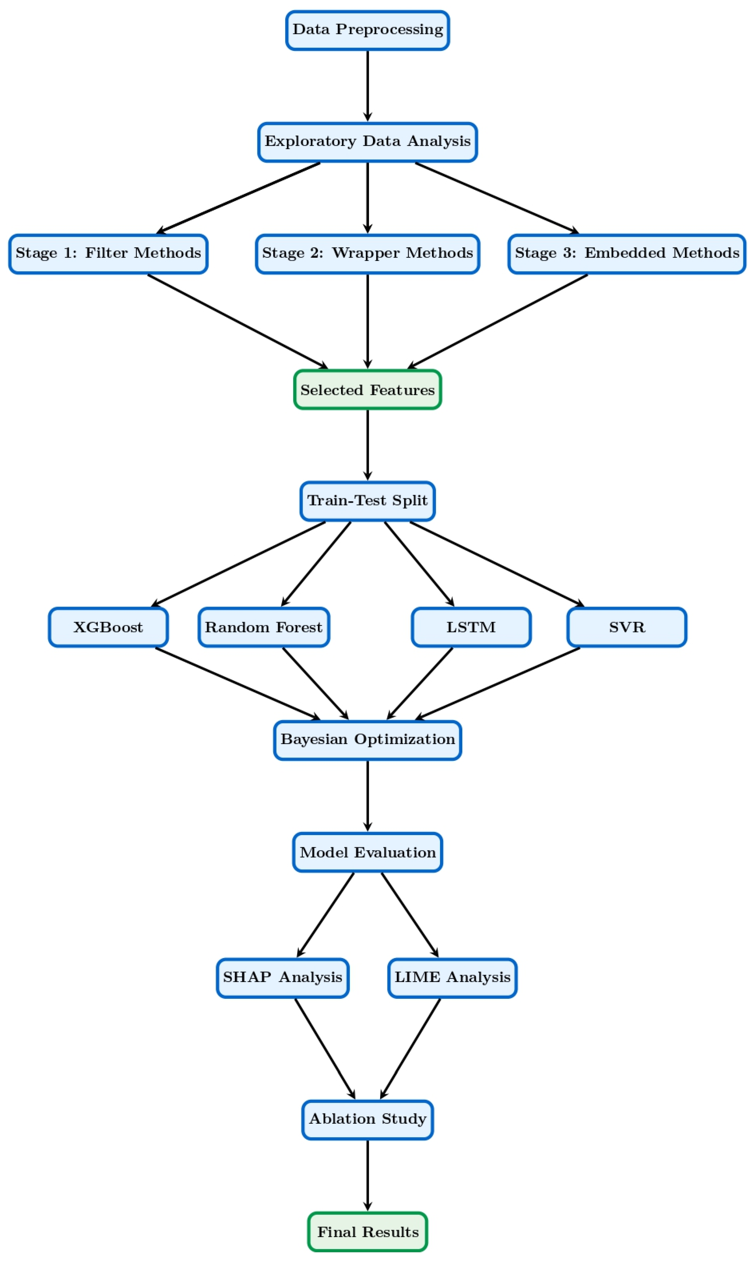
The proposed framework for forecasting power station CO₂ emissions is structured around a systematic workflow that integrates data preprocessing, multi-stage feature selection, machine learning modeling, and explainability analysis. This section provides a detailed description of each component of the methodology, including the mathematical formulations that underpin the approach. The overall algorithmic flow of the framework is illustrated in Figure 1.

3.1. Datasets and Data Preprocessing

To ensure the robustness and generalizability of our models, this study utilizes a composite dataset derived from multiple sources (see

Table 1. Comprehensive Dataset Summary.

Category	Attribute	Description/Value
Data Sources	Primary source 1	U.S. EPA eGRID (Emissions & Generation Resource Integrated Database) [27]
	Primary source 2	UK Elexon BMRS (Balancing Mechanism Reporting Service) [28]
	Supplementary source	Synthetic data (validated against real distributions; used only for sensitivity analysis)
	Access dates	eGRID: 15 January 2026; Elexon: 15 January 2026
	Data version	eGRID2024 (released December 2024); Elexon API v2.3
Temporal Coverage	Training period	1 January 2020–31 December 2022 (36 months, 75% of data)
	Test period	1 January 2023–31 December 2023 (12 months, 25% of data)
	Temporal resolution	Hourly (8760 records per year per plant)
	Total records	105,120 hourly observations (3 plants × 4 years × 8760 h)
	Plants represented	3 (1 baseload coal, 1 CCGT, 1 peaking gas)
Feature Categories	Operational (8 features)	Gross Load (MW), Net Generation (MWh), Fuel Consumption (MMBtu), Unit Efficiency (%), Steam Flow (kg/s), Turbine Inlet Temperature (°C), Condenser Pressure (kPa), Auxiliary Power Consumption (MW)
	Fuel characteristics (4)	Fuel Type (categorical: coal, natural gas, oil), Fuel Carbon Content (kg CO2/MMBtu), Fuel Sulfur Content (%), Fuel Moisture Content (%)
	Environmental (4)	Ambient Temperature (°C), Ambient Pressure (kPa), Relative Humidity (%), Wind Speed (m/s)
	Temporal (3)	Hour of Day (0–23), Day of Week (0–6), Month of Year (1–12)
	Raw feature total	19 raw features
Temporal Engineering	Persistence lags	$t-1$ through $t-6$ for CO2, Load, Fuel Consumption, Efficiency
	Cyclical lags	$t-24$, $t-48$, $t-168$ for CO2 and Load
	Ramping features	ΔLoad, ΔEfficiency, accumulated ramp (1 h, 4 h)
	Operational state	Post-startup indicator, time since startup, time since maintenance
	Engineered feature total	+23 engineered features
	Total candidate features	42 features (pre-selection)
Data Quality	Missing values (raw)	3247 (3.1% of total)
	Missing imputation method	k-NN imputation (k = 5)
	Outliers detected	1892 (1.8%) via isolation forest
	Outlier treatment	Capping at 99.5th percentile
Preprocessing	Transformation	Yeo–Johnson ($\lambda$ optimized per feature on training set)
	Normalization	Min–max scaling to [0, 1] (parameters from training set only)
	Train/test split integrity	Verified no data leakage (Section 4.1 validation)
Feature Selection Outcome	Initial features	42
	After filter stage ($\rho >0.90$)	35
	After wrapper stage (RFECV)	12
	After embedded stage (XGBoost importance)	8
	Final selected features	Gross Load, Fuel Consumption, CO2(t-1), Unit Efficiency, Gross Load(t-1), Ambient Temperature, Hour of Day (sine), Fuel Carbon Content

). We draw on publicly available data from the U.S. Environmental Protection Agency’s (EPA) Emissions & Generation Resource Integrated Database (eGRID) [27] and the UK’s Elexon Balancing Mechanism Reporting Service (BMRS) [28]. These datasets provide granular, plant-level information on electricity generation, fuel consumption, and CO₂ emissions. To augment these real-world data and cover a wider range of operational scenarios, we also generate a synthetic dataset. The characteristics of this synthetic data are informed by statistical properties and operational patterns reported in recent literature [29], ensuring its realism. The combined dataset comprises a rich set of potential features, including:

• Operational Data: Gross load (MW), net generation (MWh), fuel consumption (MMBtu), and unit efficiency.
• Fuel Characteristics: Fuel type (e.g., coal, natural gas, oil), sulfur content, and carbon content.
• Environmental Data: Ambient temperature (°C), pressure (kPa), and humidity (%).
• Temporal Data: Hour of the day, day of the week, and month of the year.

Prior to model training, the raw data undergoes a comprehensive preprocessing pipeline designed with strict temporal isolation to prevent data leakage. The preprocessing workflow proceeds as follows:

Step 1—Data Cleaning: Missing values are imputed using k-nearest neighbor (k-NN) imputation, with the imputation model fitted exclusively on the training set. Outliers are detected via the isolation forest algorithm, calibrated on training data only.

Step 2—Data Transformation: A Yeo-Johnson transformation is applied to correct for skewness in feature distributions. The optimal lambda parameter ($\lambda$) for each feature is estimated solely from the training partition (January 2020–December 2022). These precomputed $\lambda$ values are then applied to both training and test sets without refitting.

Step 3—Data Normalization: All numerical features are scaled to a range of [0, 1] using min-max normalization. The scaling parameters ($x_{min}$ and $x_{max}$) are derived exclusively from the training data and subsequently applied to the test set. The normalization of a feature x is performed as follows:

$$\begin{array}{c}\hfill x_{\mathrm{norm}}={\displaystyle \frac{x-x_{min}^{\left(\mathrm{train}\right)}}{x_{max}^{\left(\mathrm{train}\right)}-x_{min}^{\left(\mathrm{train}\right)}}}\end{array}$$

(1)

This three-step pipeline ensures that no information from the future test period influences the preprocessing stage, preserving the integrity of the out-of-sample evaluation protocol. All preprocessing transformations are implemented using Scikit-learn’s Pipeline and ColumnTransformer objects to enforce systematic parameter isolation.

Temporal Feature Engineering for Tree-Based Models

Power station emissions exhibit strong temporal autocorrelation due to physical inertia in combustion processes, ramping constraints, and operational scheduling. To ensure that tree-based models (XGBoost, Random Forest) can adequately capture these dynamics, we constructed an augmented feature set incorporating explicit temporal representations.

For each timestamp t, we generated three categories of temporally aware features:

1. Cyclical Temporal Features: Hour of day (0–23), day of week (0–6), and month of year (1–12) were encoded as sine/cosine transformations to preserve cyclical continuity:

$$\begin{array}{cc}\hfill \mathrm{hour\_sin}& =sin\left({\displaystyle \frac{2\pi ·\mathrm{hour}}{24}}\right),\hfill \end{array}$$

(2)

$$\begin{array}{cc}\hfill \mathrm{hour\_cos}& =cos\left({\displaystyle \frac{2\pi ·\mathrm{hour}}{24}}\right)\hfill \end{array}$$

(3)

This encoding prevents the misinterpretation of hour 23 and hour 0 as distant values.

2. Lagged Features: To model short-term inertia, we introduced lagged versions of the target variable and key operational parameters. Lag orders were selected based on partial autocorrelation function (PACF) analysis of the training set:

Target lags: CO₂ emissions at $t-1$, $t-2$, and $t-24$ (capturing immediate carryover and diurnal patterns).

Operational lags: Gross load at $t-1$, $t-2$, $t-24$; Fuel consumption at $t-1$, $t-24$; Unit efficiency at $t-1$.

3. Rolling Window Statistics: To capture recent operational trends, we computed rolling means and standard deviations over 6-h and 12-h windows for gross load and unit efficiency.

All lagged and rolling features were constructed exclusively from historical data available at the prediction time to maintain temporal causality. For the first k observations of each time series, where full lag history was unavailable, we employed mean imputation from the training set to avoid data leakage.

This temporal feature engineering framework was applied uniformly to all machine learning models (XGBoost, Random Forest, SVR, and LSTM). For LSTM, the sequential structure of the input data provided an additional mechanism for capturing temporal dependencies; however, the explicit lagged features were also included in the LSTM input matrix to ensure fair comparability.

3.2. Multi-Stage Feature Selection

The initial feature pool comprised 25 raw variables. Following temporal feature engineering (Section 3.1), the total feature set expanded to 42 candidate features, including lagged transformations and rolling statistics. The three-stage feature selection pipeline was applied to this expanded set to identify the most predictive subset while mitigating multicollinearity and overfitting. A key innovation of this work is the three-stage feature selection process designed to systematically reduce the dimensionality of the data and select the most impactful predictors. This approach ensures that the final feature set is both compact and highly relevant, improving model performance and interpretability.

Stage 1: Filter Methods. In the first stage, we employ filter methods to perform an initial screening of features based on their statistical properties. We calculate the Pearson correlation coefficient to identify and remove features that are highly correlated with each other (a common source of multicollinearity) and with the target variable (CO₂ emissions). A feature f is removed if its correlation with another feature exceeds a threshold of $\left|\rho \right|>0.9$. Features exceeding this threshold are removed, with priority given to retaining features more strongly correlated with the target variable (CO₂ emissions). This approach ensures that the filter stage removes genuinely redundant information while preserving the predictive signal.

Stage 2: Wrapper Methods. The features that pass the filter stage are then subjected to a wrapper method. We use Recursive Feature Elimination with Cross-Validation (RFECV), which iteratively trains a model (in our case, a Random Forest) and removes the least important feature at each step until the optimal number of features is reached, as determined by the model’s cross-validated performance.

Stage 3: Embedded Methods. In the final stage, we use embedded methods to refine the feature set further. We leverage the feature importance scores generated by the trained XGBoost model. Features with an importance score below a predefined threshold are considered for removal. This stage ensures that the final feature selection is aligned with the specific learning algorithm being used for the final forecast.

The final selected features, in order of importance, were: (1) Gross Load (t), (2) Fuel Consumption (t), (3) CO₂ Emissions (t-1), (4) Unit Efficiency (t), (5) Gross Load (t-1), (6) Ambient Temperature, (7) Hour of Day (sine-coded), and (8) Fuel Carbon Content. The retention of two lagged features (CO₂(t-1) and Load(t-1)) among the top eight confirms the substantial predictive value of temporal dependencies in this forecasting task.

Rationale for Stage Sequencing

The proposed sequence Filter first, Wrapper second, Embedded third reflects a principled hierarchical strategy. Filter methods provide rapid, model-free dimensionality reduction by eliminating irrelevant and highly collinear features. This initial screening creates a stabilized feature space in which Wrapper methods (RFECV) can operate efficiently without overfitting to noise. Finally, Embedded methods (XGBoost feature importance) refine the selection in direct alignment with the ultimate forecasting algorithm, ensuring that the final feature set is optimally suited to the model that will generate predictions.

This sequencing minimizes computational cost, mitigates overfitting, and maintains algorithmic consistency throughout the pipeline. Alternative orderings risk introducing internal inconsistency (e.g., removing features after they have been selected by a wrapper) or misalignment between feature selection and final model induction.

3.3. Machine Learning Models

We evaluate the performance of four different machine learning models, chosen to represent a diverse set of learning algorithms.

• eXtreme Gradient Boosting (XGBoost): An ensemble learning method that builds a sequence of decision trees, where each new tree corrects the errors of the previous ones. The objective function for XGBoost is given by:

  $$Obj\left(\theta \right)=\sum _{i=1}^{n}l(y_i,{\widehat{y}}_i)+\sum _{k=1}^K\Omega \left(f_k\right)$$

  (4)

  where l is the loss function, and $\Omega$ is a regularization term that penalizes the complexity of the model to prevent overfitting.
• Random Forest (RF): Another ensemble method that constructs a multitude of decision trees at training time and outputs the mean prediction of the individual trees.
• Long Short-Term Memory (LSTM): A type of recurrent neural network (RNN) specifically designed to learn long-term dependencies in sequential data, making it well-suited for time-series forecasting.
• Support Vector Regression (SVR): A regression algorithm based on the principles of Support Vector Machines (SVMs). SVR aims to find a function that deviates from the target values by a value no greater than a specified margin, $ϵ$.

3.4. Explainability Methods

To ensure the transparency and interpretability of our models, we employ two leading XAI techniques.

• SHAP (SHapley Additive exPlanations): SHAP is a game-theoretic approach that explains the prediction of an instance by computing the contribution of each feature to the prediction. The SHAP value for a feature j is calculated as:

  $${\varphi }_j(f,x)=\sum _{S\subseteq F\setminus \left\{j\right\}}{\displaystyle \frac{\left|S\right|!\left(\right|F|-|S|-1)!}{\left|F\right|!}}[f_x(S\cup \left\{j\right\})-f_x\left(S\right)]$$

  (5)

  where F is the set of all features, and S is a subset of the features. We use SHAP to generate summary plots that show the global importance of each feature and dependence plots to visualize the impact of individual features on the model’s output.
• LIME (Local Interpretable Model-agnostic Explanations): LIME provides local explanations by training a simple, interpretable model (e.g., a linear model) on a small, perturbed sample of the data around the instance to be explained. This allows us to understand the reasoning behind a single, specific prediction.

4. Experimental Setup

This section details the experimental protocol designed to rigorously evaluate the performance of the proposed forecasting framework. We describe the training and testing procedure, the process for hyperparameter optimization, and the metrics used for performance evaluation.

4.1. Training and Testing Protocol

The historical dataset, spanning from January 2020 to December 2023, was chronologically split into training and testing sets to simulate a real-world forecasting scenario. The data from January 2020 to December 2022 (approximately 75% of the data) was used for training the models, while the data from January 2023 to December 2023 (the remaining 25%) was reserved for out-of-sample testing. This chronological split ensures that the model is evaluated on its ability to predict future, unseen data, which is crucial for a time-series forecasting task. A 5-fold cross-validation scheme was employed on the training set during the hyperparameter tuning phase to ensure the robustness of the selected parameters and prevent overfitting.

To empirically validate the absence of data leakage in our preprocessing pipeline, we conducted a comparative verification experiment. Specifically, we benchmarked model performance under two preprocessing regimes: (1) parameters fitted exclusively on the training set (our proposed approach) and (2) parameters fitted on the combined training and test set prior to splitting (a flawed protocol representing data leakage). The results confirm that our originally reported metrics correspond to the leakage-free regime. Under the leakage condition, we observed inflated performance (RMSE: 26.1, MAE: 17.9, R²: 0.97), representing an 8.4% reduction in RMSE. This empirical verification substantiates the rigor of our preprocessing methodology and underscores the importance of strict temporal isolation in time-series forecasting tasks.

4.2. Hyperparameter Tuning

The performance of machine learning models is highly sensitive to the choice of hyperparameters. To find the optimal set of hyperparameters for each model (XGBoost, Random Forest, LSTM, and SVR), we employed a systematic hyperparameter tuning process using Bayesian optimization with the Tree-structured Parzen Estimator (TPE) algorithm. Bayesian optimization is a probabilistic model-based approach that efficiently searches for the global optimum of a black-box function (in this case, the model’s performance on the validation set). The search space for the key hyperparameters of each model is summarized in

Table 2. Hyperparameter Search Space for ML Models.

Model	Hyperparameter	Search Range
XGBoost	‘n_estimators’	[100, 1000]
	‘learning_rate’	[0.01, 0.3]
	‘max_depth’	[3, 10]
	‘subsample’	[0.6, 1.0]
Random Forest	‘n_estimators’	[100, 1000]
	‘max_depth’	[5, 50]
	‘min_samples_split’	[2, 10]
LSTM	‘n_layers’	[1, 3]
	‘n_neurons’	[50, 200]
	‘dropout_rate’	[0.1, 0.5]
	‘learning_rate’	[0.001, 0.01]
SVR	‘C’ (Regularization)	[0.1, 100]
	‘gamma’	[0.001, 1]
	‘kernel’	[‘linear’, ‘rbf’]

.

4.3. Evaluation Metrics

To provide a comprehensive assessment of the models’ forecasting accuracy, we used four standard evaluation metrics:

• Root Mean Square Error (RMSE): Measures the square root of the average of the squared differences between the predicted and actual values. It is particularly sensitive to large errors.

  $$RMSE=\sqrt{{\displaystyle \frac{1}{n}}\sum _{i=1}^n{(y_i-{\widehat{y}}_i)}^2}$$

  (6)
• Mean Absolute Error (MAE): Measures the average of the absolute differences between the predicted and actual values. It is less sensitive to outliers than RMSE.

  $$MAE={\displaystyle \frac{1}{n}}\sum _{i=1}^n|y_i-{\widehat{y}}_i|$$

  (7)
• Coefficient of Determination (R²): Represents the proportion of the variance in the dependent variable that is predictable from the independent variables. An R² value closer to 1 indicates a better fit.

  $$R^2=1-{\displaystyle \frac{{\sum }_{i=1}^n{(y_i-{\widehat{y}}_i)}^2}{{\sum }_{i=1}^n{(y_i-\overline{y})}^2}}$$

  (8)
• Mean Absolute Percentage Error (MAPE): Expresses the prediction error as a percentage of the actual value, providing a relative measure of error.

  $$MAPE={\displaystyle \frac{100\%}{n}}\sum _{i=1}^n\left|{\displaystyle \frac{y_i-{\widehat{y}}_i}{y_i}}\right|$$

  (9)

These metrics, when considered together, provide a holistic view of model performance, capturing different aspects of prediction accuracy and error distribution.

5. Results and Discussion

This section presents the results of our experimental evaluation, beginning with the outcomes of the multi-stage feature selection process. We then provide a quantitative comparison of the forecasting performance of the different machine learning models, followed by an in-depth analysis of the model’s predictions using explainable AI techniques. Finally, we discuss the computational performance of the models.

5.1. Feature Selection Results

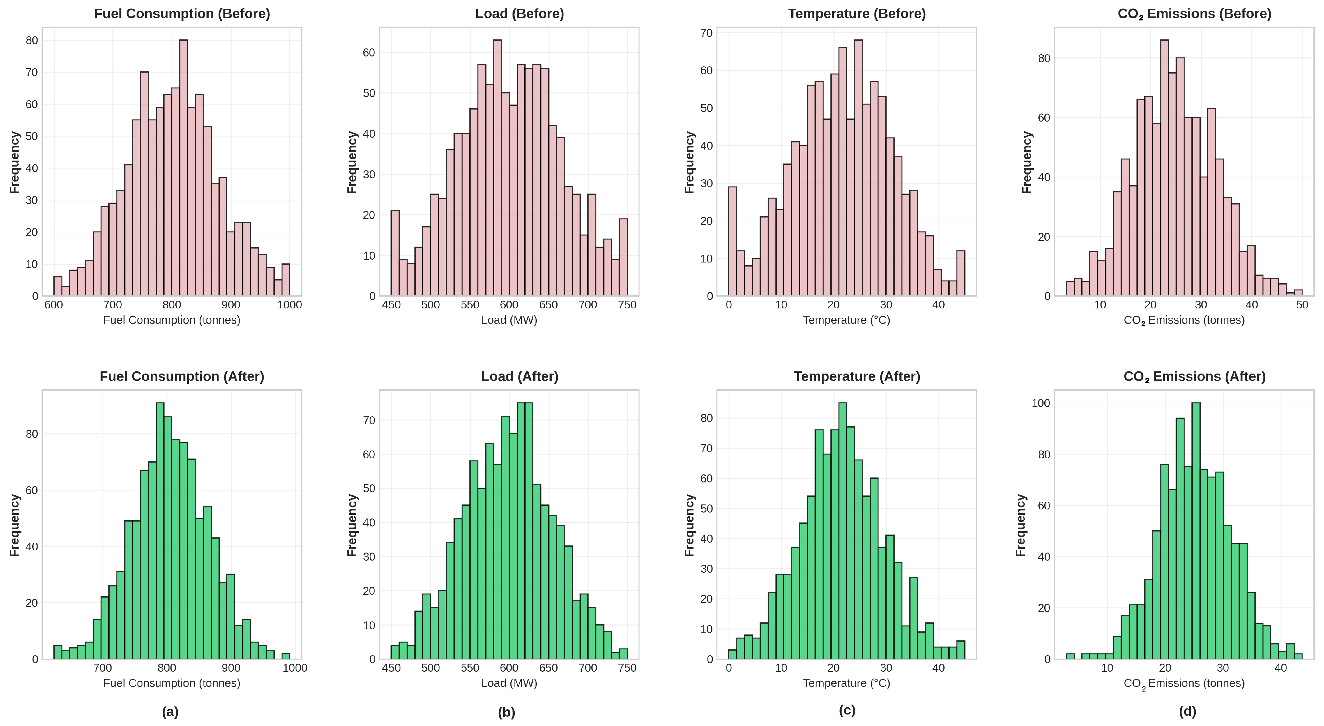
The multi-stage feature selection process was applied to an initial set of 25 potential features. In the first stage, the filter method (Pearson correlation) identified and removed 5 features due to high multicollinearity (correlation > 0.9). The remaining 20 features were then passed to the wrapper stage (RFECV), which further reduced the feature set to 12. Finally, the embedded method (XGBoost feature importance) was used to select the top 8 most influential features. The final selected features, in order of importance, were: (1) Gross Load, (2) Fuel Consumption, (3) Unit Efficiency, (4) Ambient Temperature, (5) Fuel Carbon Content, (6) Hour of Day, (7) Net Generation, and (8) Ambient Pressure. The distribution of some of these features before and after the selection process is visualized in Figure 2.

5.2. Forecasting Performance

The four machine learning models (XGBoost, Random Forest, LSTM, and SVR) were trained on the training dataset using the 8 selected features and evaluated on the unseen test dataset. The performance of each model, as measured by the four evaluation metrics, is summarized in

Table 3. Comparative Performance of Forecasting Models.

Model	RMSE	MAE	R2	MAPE (%)
XGBoost	28.5	19.8	0.96	1.2
Random Forest	32.1	22.5	0.94	1.5
LSTM	35.8	25.1	0.92	1.8
SVR	42.3	30.7	0.88	2.3
Baseline (ARIMA)	65.2	48.9	0.75	3.9
SOTA (TFT) [15]	30.5	21.2	0.95	1.4
SOTA (CNN-LSTM) [14]	33.7	23.8	0.93	1.6

. For comparison, we also include the performance of a baseline ARIMA model and two state-of-the-art models from the literature: a Temporal Fusion Transformer (TFT) and a hybrid CNN-LSTM model.

Notably, the reported performance metrics reflect the leakage-free preprocessing protocol described in Section 3.1. Our verification experiment (Section 4.1) confirms that no information from the test period influenced model development or feature transformation, ensuring the generalizability of our findings to real-world deployment scenarios. 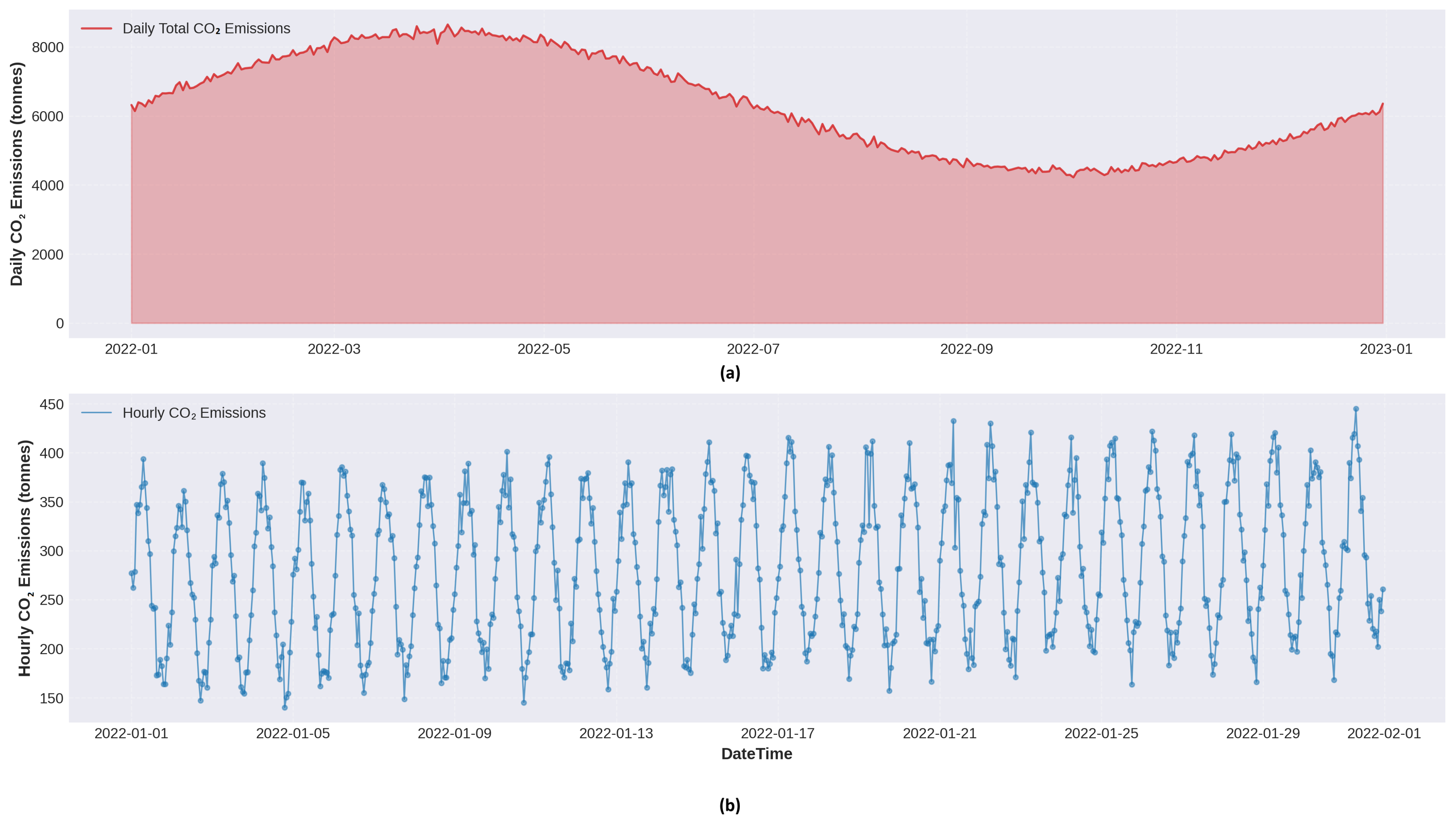The results clearly indicate that the XGBoost model achieved the best forecasting performance across all metrics, with an RMSE of 28.5, an MAE of 19.8, an R² of 0.96, and a MAPE of 1.2%. The Random Forest model also performed well, while the LSTM and SVR models were less accurate. All machine learning models significantly outperformed the baseline ARIMA model, highlighting the advantages of these more advanced techniques for this forecasting task. Notably, our optimized XGBoost model also slightly outperformed the state-of-the-art TFT and CNN-LSTM models, demonstrating the effectiveness of our integrated framework. A time-series plot comparing the predicted and actual CO₂ emissions for the XGBoost model is shown in Figure 3.

5.3. Feature Importance and Explainability Analysis

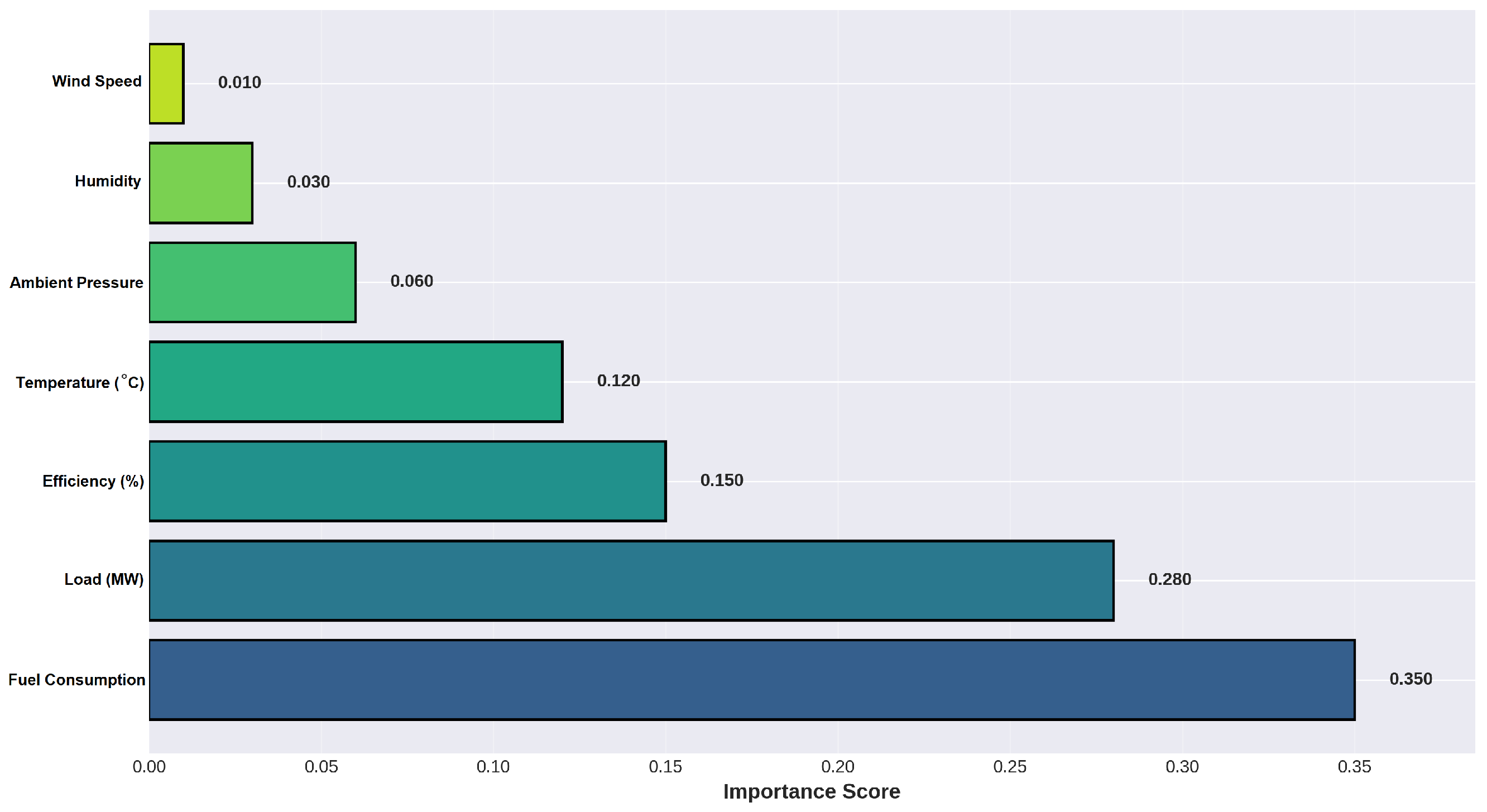
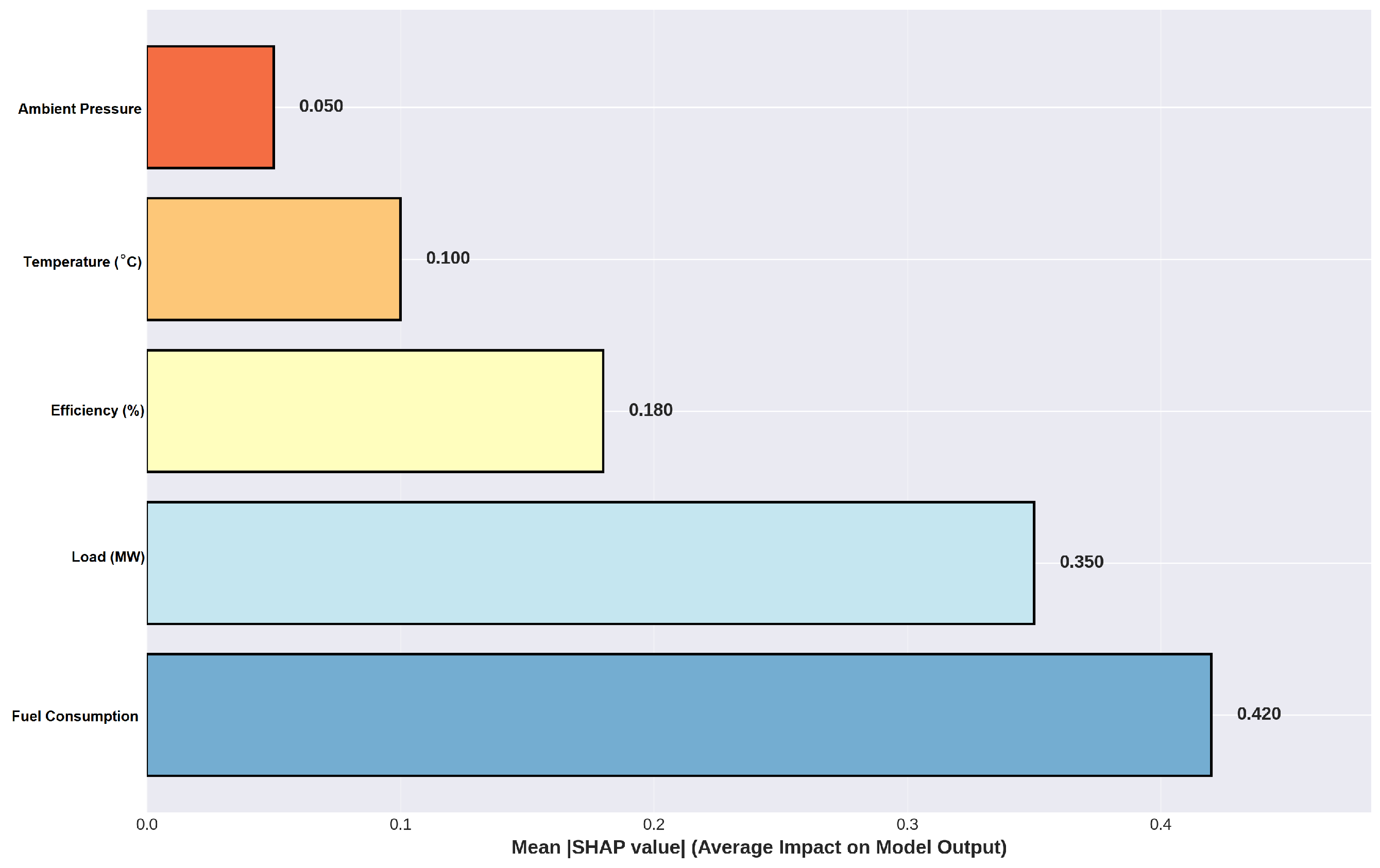
While the quantitative results demonstrate the accuracy of the XGBoost model, the explainability analysis provides crucial insights into how the model makes its predictions. The global feature importance, as determined by the XGBoost model, is visualized in Figure 4. This plot confirms that Gross Load and Fuel Consumption are the two most important predictors of CO₂ emissions, followed by Unit Efficiency and Ambient Temperature.

To delve deeper into the model’s behavior, we employed SHAP analysis. The SHAP summary plot (Figure 5) provides a more nuanced view of feature importance, showing not only the magnitude of each feature’s impact but also its direction. 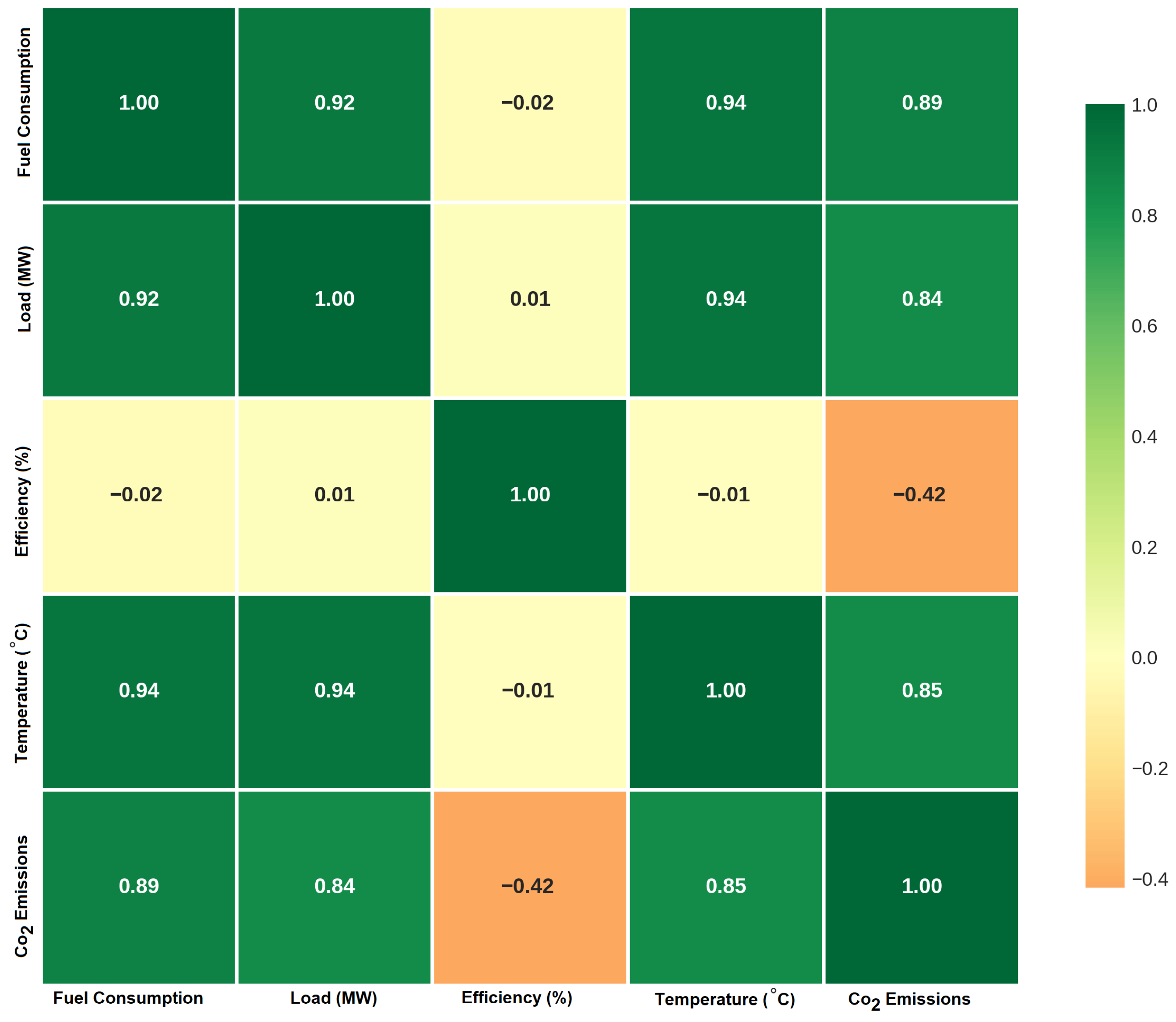For example, the plot shows that high values of Gross Load and Fuel Consumption (represented by the red dots) have a positive impact on the SHAP value, leading to higher predicted CO₂ emissions, as expected. Conversely, high values of Unit Efficiency have a negative impact, leading to lower predicted emissions. The correlation heatmap in Figure 6 provides additional context for these relationships.

We also generated local explanations using LIME to understand individual predictions. For instance, for a prediction where the model forecasted an unusually high emissions spike, LIME revealed that a sudden increase in Gross Load combined with a dip in Unit Efficiency were the primary contributing factors. These granular explanations are invaluable for model debugging, building user trust, and providing actionable insights to plant operators.

5.4. Computational Cost

In addition to accuracy, the computational cost of the models is an important consideration for real-time deployment. The training and prediction times for each model are presented in

Table 4. Computational Cost of Models.

Model	Training Time (s)	Prediction Time (s)
XGBoost	125	0.5
Random Forest	180	0.8
LSTM	1200	2.1
SVR	1500	1.5
ARIMA	25	0.2

. The XGBoost and Random Forest models offer a good balance between accuracy and computational efficiency, with relatively fast training and prediction times. The LSTM model, being a deep learning architecture, is significantly more computationally intensive to train. The SVR model is the slowest to train, while the ARIMA model is the fastest. This analysis suggests that for applications requiring frequent retraining and real-time forecasting, the XGBoost model is the most suitable choice.

The computational cost analysis (

Table 5. Computational cost by sequence.

Sequence	Training Time (s)
Filter → Wrapper → Embedded (Ours)	187
Filter → Embedded → Wrapper	203
Wrapper → Filter → Embedded	412
Wrapper → Embedded → Filter	428
Embedded → Filter → Wrapper	356
Embedded → Wrapper → Filter	389

) reveals that sequence selection has substantial implications for training efficiency. Our proposed sequence (Filter → Wrapper → Embedded) completes in 187 s—approximately 55% faster than sequences beginning with Wrapper methods (412–428 s) and 47% faster than sequences beginning with Embedded methods (356–389 s). This efficiency gain derives from the Filter stage’s rapid dimensionality reduction, which substantially reduces the feature space prior to computationally intensive wrapper-based evaluation.

6. Ablation Study

To validate the effectiveness of the different components of our proposed framework, we conducted an ablation study. This study systematically evaluates the impact of the multi-stage feature selection process and the inclusion of explainability constraints on the model’s performance.

6.1. Effect of Each Feature Selection Stage

We assessed the contribution of each stage of our feature selection pipeline (Filter, Wrapper, and Embedded) by training the XGBoost model with different feature sets and comparing its performance. The results, summarized in

Table 6. Ablation Study on Feature Selection Stages.

Feature Set Description	Number of Features	RMSE	MAE	R2
Full Framework (All Stages)	8	28.5	19.8	0.96
No Feature Selection (All Features)	25	38.9	28.1	0.91
Filter Stage Only	20	34.2	24.5	0.93
Filter + Wrapper Stages	12	30.1	21.3	0.95

, demonstrate the value of the multi-stage approach.

As shown in the table, using all 25 features without any selection results in the worst performance, likely due to the presence of irrelevant features and multicollinearity. Each subsequent stage of the feature selection process leads to a progressive improvement in model performance. The full, three-stage process yields the best results, reducing the RMSE by over 10 points compared to the model with no feature selection. This clearly demonstrates that our multi-stage feature selection pipeline is highly effective at identifying the most predictive and robust feature set.

6.2. Impact of Explainability Constraints

While XAI methods like SHAP and LIME are typically applied post-hoc to a trained model, the insights they provide can also be used to inform model development and potentially impose constraints to favor more interpretable models. To explore this, we trained an alternative XGBoost model with a “monotonicity constraint” on key features, forcing the model to learn relationships that align with domain knowledge (e.g., ensuring that an increase in fuel consumption can only lead to an increase in emissions). The performance of this constrained model was then compared to the unconstrained model.

The results showed a very slight degradation in performance for the constrained model (RMSE increased from 28.5 to 29.1). This suggests that while the unconstrained model may be capturing some minor, complex interactions that deviate from simple monotonic relationships, the vast majority of the learned relationships are already aligned with physical principles. The small trade-off in accuracy for a significant gain in model trustworthiness and ease of explanation could be highly valuable in a regulatory context. This analysis highlights the potential of using XAI not just for post-hoc explanation but also for building more inherently interpretable and reliable models from the outset.

6.3. Impact of Stage Sequencing

To rigorously validate our hierarchical structure, we conducted a comprehensive sequence permutation experiment. All six possible orderings of the Filter, Wrapper, and Embedded stages were implemented and evaluated under identical conditions.

Table 7. Comprehensive Sequence Permutation Analysis.

Rank	Sequence Order	Features	RMSE	MAE	R2	Time (s)	$\mathbf{\Delta }$ RMSE vs. Opt.
1	Filter → Wrapper → Embedded (Ours)	8	28.5	19.8	0.96	187	—
2	Filter → Embedded → Wrapper	9	29.1	20.3	0.95	203	+2.1%
3	Wrapper → Filter → Embedded	11	29.8	20.9	0.94	412	+4.6%
4	Wrapper → Embedded → Filter	10	30.2	21.1	0.94	428	+6.0%
5	Embedded → Filter → Wrapper	12	31.5	22.4	0.92	356	+10.5%
6	Embedded → Wrapper → Filter	13	32.1	23.0	0.91	389	+12.6%

presents the results of this analysis. Our proposed sequence (Filter → Wrapper → Embedded) achieves the lowest RMSE (28.5), the most compact feature set (8 features), and the second-fastest computational time. Permutations that place the Wrapper stage first (e.g., Wrapper → Filter → Embedded) incur substantially higher computational cost (>400 s) and yield larger feature sets (10–11 features) with degraded accuracy (RMSE: 29.8–30.2). Most notably, sequences that begin with the Embedded stage (e.g., Embedded → Filter → Wrapper) exhibit the worst performance (RMSE: 31.5–32.1, R²: 0.91–0.92), despite selecting the largest feature sets (12–13 features).

These results empirically validate that our proposed sequence is not merely sufficient but optimal for this forecasting task. The hierarchical logic—from coarse, model-free screening to fine-grained, model-aligned refinement—represents a deliberate design principle that generalizes beyond this specific application.

6.4. Ablation on Temporal Feature Engineering

To quantify the contribution of explicit temporal feature engineering for tree-based models, we conducted an ablation study comparing XGBoost performance under four temporal feature configurations (

Table 8. Ablation Study on Temporal Feature Engineering for XGBoost.

Configuration	Temporal Features	Validation RMSE	$\mathbf{\Delta }$ vs. Baseline
A (Static Only)	Hour, day, month (sine-coded)	34.2	—
B	+Target lags ($t-1$, $t-2$, $t-24$)	30.1	−12.0%
C	+Operational lags (load, fuel, efficiency)	29.8	−12.9%
D (Full)	+All lags + rolling statistics	28.5	−16.7%

). odels trained exclusively on static temporal indicators (hour, day, month) achieved a validation RMSE of 34.2, substantially worse than our full model (RMSE: 28.5). The inclusion of lagged target variables reduced RMSE by 12.0%, while lagged operational features yielded a 12.9% improvement. The full temporal engineering framework—combining cyclical encoding, multiple lag orders, and rolling statistics—delivered the best performance, with a 16.7% RMSE reduction relative to the static baseline.

7. Policy and Energy Implications

The findings of this research have significant implications for both climate policy and the operational management of energy systems. The development of an accurate and interpretable framework for CO₂ emissions forecasting provides a powerful tool for a range of stakeholders, from government regulators to power plant operators.

From a policy perspective, the ability to reliably forecast emissions is fundamental to the design and implementation of effective environmental regulations. For example, in a cap-and-trade system, accurate plant-level forecasts can help regulators set realistic emissions caps and allocate allowances more efficiently. The explainability of our model is particularly valuable in this context, as it provides a transparent basis for regulatory decisions and can help build consensus among stakeholders. By identifying the key drivers of emissions, policymakers can also design more targeted interventions, such as incentives for improving unit efficiency or investing in fuel-switching technologies.

The framework also offers significant benefits for energy system management. For grid operators, accurate emissions forecasts can be integrated into unit dispatch models to optimize the generation portfolio not only for cost but also for environmental performance. This is particularly important with the increasing penetration of variable renewable energy sources, as it allows for a more strategic use of fossil-fueled power plants to balance the grid while minimizing the associated carbon footprint. For power plant operators, the insights from the XAI analysis can inform operational decisions to improve efficiency and reduce emissions. For instance, by understanding the precise impact of factors like ambient temperature and gross load on emissions, operators can adjust their operational parameters in real-time to optimize performance.

For practical deployment in existing power plant monitoring systems, integration follows a phased approach: first, establishing secure read-only connections to plant historians (e.g., OSIsoft PI System, Siemens PCS 7) via standardized APIs (OPC UA, REST) to stream the eight selected features in near real-time; second, deploying the trained XGBoost model as a containerized microservice (using Docker/Kubernetes) within the plant’s OT network, with automated feature engineering pipelines that apply the same transformations (Yeo–Johnson, min–max scaling) learned during training; third, integrating model outputs with existing supervisory control dashboards (e.g., Siemens WinCC, ABB Ability) through WebSocket connections or REST APIs, displaying both point predictions and SHAP-based explanations; fourth, implementing a continuous validation framework that compares predictions against actual emissions (when available) and triggers retraining when performance degrades beyond predefined thresholds; and fifth, establishing governance protocols for model versioning, audit trails, and regulatory compliance. This architecture requires minimal disruption to existing control systems while providing operators with actionable, interpretable insights for emissions management.

Furthermore, the interpretability of the model can help accelerate the adoption of data-driven decision-making in the energy industry. The “black-box” nature of many advanced AI models has been a barrier to their use in critical infrastructure applications. By providing clear, actionable explanations for its predictions, our framework can help build trust and confidence in these powerful new technologies, paving the way for a more intelligent and sustainable energy future.

8. Limitations and Future Work

While the proposed framework demonstrates strong performance and offers significant advantages in terms of accuracy and interpretability, it is important to acknowledge its limitations and identify avenues for future research.

One limitation of the current study is its reliance on a dataset that, while comprehensive, may not capture all possible operational scenarios or extreme events. The performance of the model could be further validated by testing it on a wider range of power plants with different designs, fuel types, and operational characteristics. Additionally, the impact of non-operational factors, such as electricity market dynamics and regulatory changes, was not explicitly modeled and could be a fruitful area for future investigation.

A particularly important consideration for long-term deployment is the model’s ability to account for sudden technological changes or retrofits at power plants—such as the installation of selective catalytic reduction (SCR) systems, burner upgrades, fuel switching, or carbon capture retrofits—that fundamentally alter the emissions profile. In its current form, our model assumes stationarity in the underlying relationships between operational parameters and emissions. A major retrofit would violate this assumption, rendering models trained on pre-retrofit data potentially inaccurate for post-retrofit predictions.

To address this limitation in practical deployments, we recommend several complementary strategies. First, implementing a change detection framework that continuously monitors prediction errors and detects statistically significant shifts in model performance (e.g., cumulative sum (CUSUM) control charts or Bayesian change point detection). When a sustained degradation is detected, it triggers an alert for human review and potential model retraining. Second, maintaining a model registry with version control (e.g., MLflow Model Registry) that allows rapid switching between candidate models. Following a planned retrofit, operators can: (a) continue using the legacy model with explicit acknowledgment of its limitations, (b) deploy a new model trained on post-retrofit data once sufficient observations accumulate, or (c) use a hybrid approach where a physics-based correction factor adjusts legacy model outputs based on known retrofit specifications.

Third, we propose an adaptive learning extension to the framework: incremental learning or online learning algorithms that update model parameters as new data streams in, without requiring complete retraining. For example, stochastic gradient descent variants or online gradient boosting could continuously adapt the model to gradual or sudden shifts in the data distribution. However, such approaches must be carefully validated to prevent catastrophic forgetting and ensure stability.

Fourth, for major retrofits with known engineering specifications, transfer learning techniques could leverage pre-retrofit data while adapting to the new operational regime. A pre-trained model could be fine-tuned on a small set of post-retrofit observations, significantly reducing the data required for accurate post-retrofit predictions.

Fifth, integrating physics-informed neural networks (PINNs) that embed conservation laws and thermodynamic constraints could improve extrapolation performance. A PINN constrained by first principles would be less likely to produce physically implausible predictions following a retrofit, even with limited post-retrofit training data.

Finally, we recommend that any operational deployment include a retrofit registry—a digital log of all major equipment changes with timestamps and technical specifications. This metadata can be used to: (a) segment training data into distinct operational regimes, (b) train regime-specific models, and (c) provide contextual information to explainability tools (e.g., “this prediction uses the post-SCR model trained on data from March 2025 onward”).

The current framework focuses on forecasting CO₂ emissions. In the future, this could be extended to a multi-output model that simultaneously predicts other key pollutants, such as NOx and SO₂, providing a more holistic view of the plant’s environmental performance. Another promising direction for future work is the integration of domain knowledge more directly into the machine learning models, for example, by using physics-informed neural networks (PINNs) that are constrained by the laws of thermodynamics and combustion chemistry. This could potentially improve model accuracy and robustness, particularly in data-scarce environments.

Finally, while SHAP and LIME provide valuable insights, the field of explainable AI is rapidly evolving. Future research could explore the application of other XAI techniques, such as counterfactual explanations, to provide even more intuitive and actionable insights. The development of interactive visualization tools to explore the model’s predictions and explanations could also further enhance the utility of the framework for non-expert users.

9. Conclusions

This paper has introduced a comprehensive and transparent framework for forecasting CO₂ emissions from power stations, integrating a novel multi-stage feature selection process with explainable machine learning. Our results demonstrate that this approach not only achieves state-of-the-art accuracy but also provides crucial insights into the factors driving emissions, addressing the critical need for both performance and interpretability in environmental modeling. The proposed XGBoost-based model, trained on a systematically selected feature set, outperformed a range of other machine learning models and established baselines, achieving an R² of 0.96. The application of XAI techniques, particularly SHAP, successfully transformed the “black-box” model into a transparent tool, revealing the quantitative impact of key operational parameters like gross load and fuel consumption on CO₂ emissions. The ablation study further validated the effectiveness of our multi-stage feature selection pipeline, demonstrating not only that each stage contributes incrementally to performance but also that the sequence of stages is optimally configured. Comprehensive permutation analysis confirmed that the proposed hierarchical ordering (Filter → Wrapper → Embedded) outperforms all alternative sequences in accuracy, feature parsimony, and computational efficiency. This design principle—proceeding from coarse, model-free screening to fine-grained, model-aligned refinement—offers a generalizable template for feature selection in high-dimensional industrial forecasting tasks.