


Abstract
To accurately characterize the complex coupling and nonlinear interactions between meteorological and oceanic variables in offshore wind power scenarios, this study proposes a novel forecasting model based on a “multi-scale fusion-decomposition-reconstruction-optimization-prediction” framework. This model integrates Variational Modal Decomposition (VMD) with the feature-interaction Informer framework, employing an enhanced Honey Badger Algorithm (HBA) for the collaborative optimization of their key parameters. The enhanced HBA integrates cubic chaotic mapping, random perturbation strategy, elite tangent search, and differential mutation operations to strengthen its global optimization capability and convergence efficiency. The model construction process proceeds as follows: First, sample entropy (SE) is applied to evaluate the entropy values and reconstruct sequences of the modal components obtained from VMD. Subsequently, the dynamic adjustment of the maximum information coefficient (DE-MIC) is employed to select key input variables from multi-source features. Subsequently, the feature interaction-probabilistic sparse attention mechanism (FI-ProbSparse-AM) unique to the feature interaction-based Informer is employed to construct an attention architecture capable of explicitly modeling dependencies among multidimensional variables, thereby effectively capturing the spatiotemporal latent correlations between wind power output and multi-source features. Experiments based on real offshore wind farm data demonstrate that the MAPE values are reduced by approximately 11% compared to existing benchmark models. The proposed method demonstrates significant advantages in both prediction accuracy and stability.
1. Introduction
With the continuous growth of global energy demand and the pollution associated with traditional fossil fuels, wind energy has garnered increasing recognition and adoption by numerous countries. Wind power generation primarily consists of onshore and offshore wind energy [1]. Given that global onshore wind technology has matured and even reached saturation in many regions, the exploitation of marine resources has become an urgent priority. Consequently, the offshore wind power industry is gradually occupying a central role in the energy landscape [2]. In recent years, continuous exploration and research in offshore wind technology have made the large-scale deployment of offshore wind farms increasingly feasible [3]. However, the marine environment is characterized by high complexity, including randomness, variability, and non-stationarity [4], which impose more demanding operating conditions on offshore wind turbines. The accuracy of wind power forecasting serves as a cornerstone for grid stability, effective coordination of electricity distribution, and reliable production planning. Therefore, ensuring high accuracy and stability in offshore wind power prediction is crucial for the advancement of offshore wind technology.
Forecasting models for offshore wind power mainly include physical models [5,6,7], statistical models [8,9,10], and artificial intelligence-based models. Among these, physical models employ Numerical Weather Prediction (NWP) to integrate various variables such as regional topography and environmental conditions for precise forecasting. Nevertheless, they often suffer from data redundancy and low prediction efficiency. Statistical models rely solely on the analysis and identification of historical power data for forecasting, yet they are limited in prediction accuracy and often lack stability.
In recent years, artificial intelligence models have demonstrated outstanding performance in the field of wind power forecasting. Techniques such as Support Vector Machine (SVM) [11], Gated Recurrent Unit (GRU) [12], and Bidirectional Long Short-Term Memory network (BiLSTM) [13] possess a strong capacity for learning complex features and addressing highly nonlinear problems, leading to their widespread adoption in wind power prediction. However, the higher stochastic volatility inherent in offshore wind power data makes feature extraction more challenging, rendering simplistic models inadequate for current demands. Attention mechanism (AM) has been extensively applied to enhance model capabilities. For instance, Xu et al. [14] integrated an attention mechanism into the multi-layer neurons of a BiGRU network, strengthening its ability to capture diverse data features and thereby improving forecast accuracy. The ProbSparse self-attention mechanism, intrinsic to the Informer model [15], excels at tasks requiring the maintenance of long-term dependencies. It demonstrates superior parallel processing capability compared to BiGRU and captures global long-range dependencies more accurately. By incorporating a multi-head probabilistic sparse self-attention mechanism, it effectively addresses the limitations of the Transformer [16], such as high memory consumption, high time complexity, and the constraints of the encoder–decoder architecture. This enables efficient extraction of historical data features, leading to a comprehensive improvement in overall performance. Huang et al. [17] proposed a multi-site, multi-modal, multi-step forecasting model based on Informer, utilizing it to resolve spatial and temporal dependency issues. The model has also exhibited strong generalization capabilities in applications such as motor bearing vibration monitoring and photovoltaic power generation forecasting [18,19]. Given the high stochasticity and nonlinear characteristics of wind power data, the use of data preprocessing techniques is particularly crucial. These methods include Wavelet Transform (WT) [20,21,22], Empirical Mode Decomposition (EMD) [23], Complete Ensemble Empirical Mode Decomposition with Adaptive Noise (CEEMDAN) [24], and Variational Mode Decomposition (VMD) [25]. However, WT, EMD, and CEEMDAN suffer from the issue of mode mixing. In contrast, VMD effectively mitigates this problem by employing Wiener filtering, center frequencies, and bandwidth constraints. Literature [26] proposed a method that employs the VMD algorithm to decompose data and utilizes the Sparrow Search Algorithm (SSA) to optimize the parameters of a TCN-BiGRU model. Experimental results confirmed the superior predictive performance of this model. Another study [27] introduced a hybrid wind power forecasting model named IVMD-FE-Ad-Informer, which combines an Informer model with an adaptive loss function, Improved Variational Mode Decomposition (IVMD), and Fuzzy Entropy (FE). This approach reconstructs the subsequences decomposed by IVMD before feeding them into the adaptive robust Ad-Informer model for prediction. The final forecast is obtained by aggregating the predicted values of each subsequence. Nonetheless, the manual configuration of VMD’s internal parameters remains largely subjective and prone to arbitrariness.
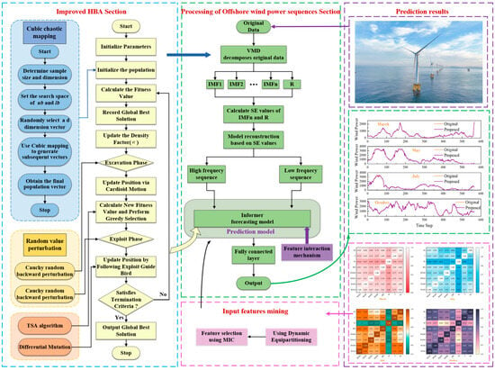
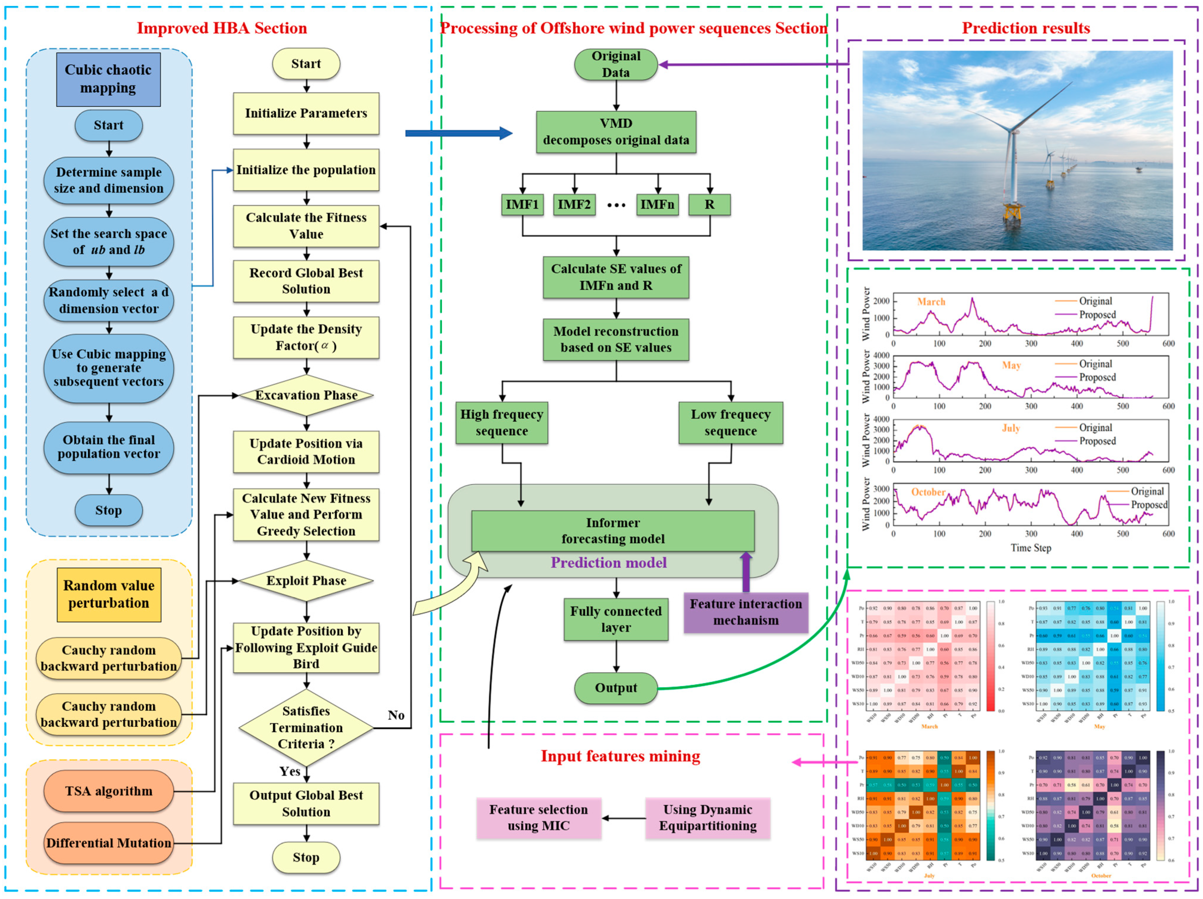
In summary, current methods for offshore wind power forecasting exhibit several limitations. Techniques employing data decomposition such as VMD and CEEMDAN often involve high computational costs and challenges in parameter configuration. Simpler models fail to effectively capture the spatiotemporal dependencies between multi-source data and power output. Furthermore, traditional optimization algorithms frequently demonstrate inefficiency and struggle to locate optimal parameters. While many approaches consider local feature correlations, they often overlook the influence of dependencies among multi-source data on the output variable. To address these gaps in decomposition parameter optimization, algorithm efficiency, and multi-modal, multi-scale representation, this paper proposes a hybrid model for offshore wind power prediction, which improves upon existing wind energy models. The proposed framework operates as follows. First, Variational Mode Decomposition (VMD) is applied to decompose the original power data into multiple scale-based sub-modes. An improved Honey Badger Algorithm (HBA) is simultaneously employed to optimize two key VMD parameters: the penalty factor and the number of decomposition modes. Subsequently, the decomposed sub-sequences are reconstructed into high-frequency and low-frequency components using the median Sample Entropy (SE) value as a threshold. Critical input features are then selected via the Dynamically Equidistant Maximal Information Coefficient (DE-MIC). Next, the high- and low-frequency sequences are fed into a Feature-Interactive Informer (FI-Informer) model for prediction. The improved HBA is again utilized to optimize six hyperparameters of the FI-Informer: feature dimension, attention mechanism computation scale, number of attention heads, feed-forward hidden layer dimension, number of encoder/decoder stacking layers, and the ProbSparse attention sampling factor. Finally, the prediction results are generated through a fully connected layer. The overall workflow of the proposed model is illustrated in Figure 1. A comparison of the methods described in the above literature with the methods used in this paper is presented in Table A1 of the Appendix A.
Figure 1.
Workflow Diagram of the IHBA-VMD-FI-Informer Model.
The innovative contributions of this paper are summarized as follows:
- (1)
- A novel offshore wind power forecasting model, termed IHBA-VMD-FI-Informer, is proposed, which integrates data decomposition techniques with a multimodal and multiscale Informer framework.
- (2)
- An Improved Honey Badger Algorithm (IHBA) is employed to optimize the penalty factor and the number of modes in the VMD process. This approach mitigates the subjectivity and blindness associated with manual parameter selection, thereby preventing the adoption of suboptimal configurations.
- (3)
- The decomposed subsequences are reconstructed into high-frequency and low-frequency components based on their Sample Entropy (SE) values. Furthermore, a modified Maximal Information Coefficient (MIC) method incorporating distribution-adjusted dynamic gridding is utilized to identify salient input features from multi-source data, enhancing the model’s forecasting efficiency.
- (4)
- The Honey Badger Optimization algorithm (HBA) is enhanced by integrating a Cubic chaotic map, a stochastic perturbation strategy, an elite tangent algorithm [28], and a differential mutation operator. These modifications strengthen its global search capability and improve its ability to escape local optima.
- (5)
- A feature interaction mechanism is incorporated into the Informer architecture to address its inherent limitation in modeling nonlinear interactions among multi-source variables. This enhancement allows the model to capture data characteristics more accurately, reduces its excessive reliance on individual features, and more effectively leverages the combined influence of multi-source data, leading to superior overall forecasting performance.
2. Methods
2.1. Variational Mode Decomposition
Variational Mode Decomposition (VMD) is a fully non-recursive and adaptive signal processing method. Its core principle is to decompose a complex, non-stationary signal into a series of quasi-orthogonal Intrinsic Mode Functions (IMFs) with sparse and limited bandwidth characteristics. The corresponding constrained variational problem is formulated as shown in Equation (1).
In Equation (1), denotes the k-th mode function, represents its center frequency, is the partial derivative with respect to time, stands for the Dirac function, K indicates the predefined total number of modes, and is the original input signal.
By introducing a quadratic penalty factor and a Lagrange multiplier , the constrained problem is transformed into an unconstrained one. The corresponding Lagrangian expression is given by Equation (2).
The iterative updates of , and are carried out using the Alternating Direction Method of Multipliers (ADMM). The specific updating formulas for each sub-problem are as follows.
In Equations (3)–(5), the symbol “^” denotes the Fourier Transform, n represents the iteration index, and τ is the update step size. The iteration process terminates once the convergence criterion specified in Equation (6) is satisfied, at which point the final IMF components in the time domain and their corresponding center frequencies are output.
In Equation (6), “ε” denotes the relative error tolerance.
2.2. Improved Honey Badger Algorithm Optimized Variational Mode Decomposition
The selection of the number of decomposition modes (K) and the penalty factor (α) is particularly crucial for improving the outcome of data decomposition. An excessively large K may produce spurious modal components, while a K that is too small can lead to mode aliasing. Similarly, an overly high penalty factor tends to suppress the intrinsic characteristics of the data, whereas an insufficient value amplifies internal signal noise.
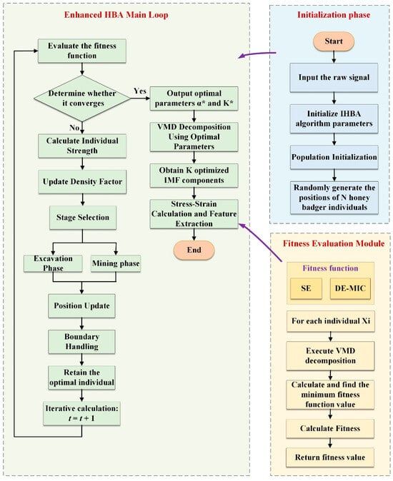
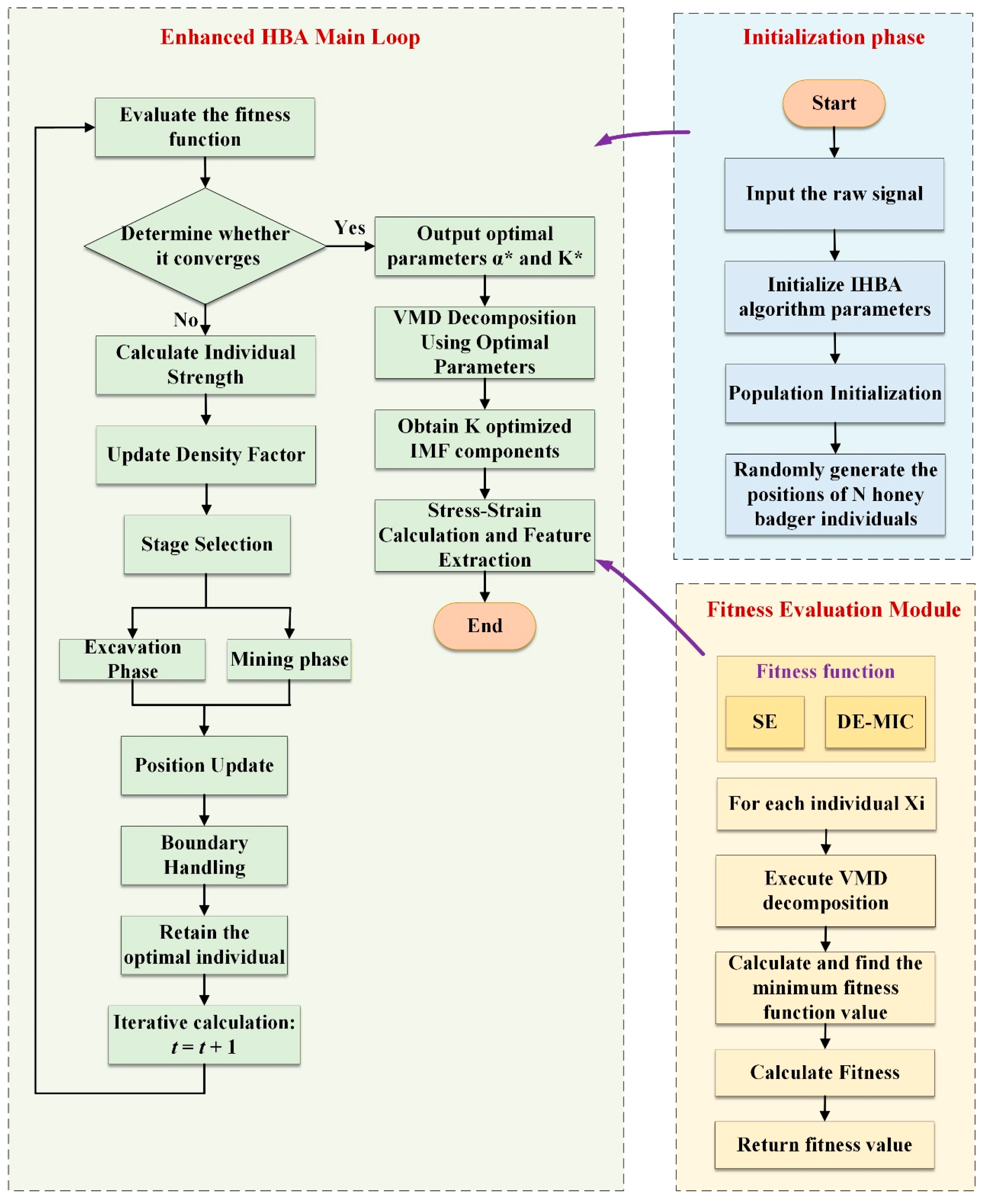
To mitigate the subjectivity and arbitrariness associated with manual parameter selection, this study employs the Improved Honey Badger Algorithm (IHBA) to optimize both the penalty factor and the number of modes in the VMD process. The technical flowchart of the IHBA-VMD optimization procedure is illustrated in Figure 2.
Figure 2.
The technical workflow of the IHBA-VMD.
2.3. Sample Entropy
Sample Entropy (SE) serves as a statistical measure for evaluating the complexity and regularity of time series, offering advantages in consistency, comparability, and independence [29]. Unlike approximate entropy or permutation entropy, SE is less influenced by the sequential order of data and effectively mitigates bias, while exhibiting stronger noise robustness. These properties make it particularly suitable for processing offshore wind power sequences, where it responds effectively to sudden fluctuations in wind generation. A higher SE value indicates greater internal complexity and variability within the sequence, which corresponds to increased forecasting difficulty. The calculation of SE is expressed in Equation (7).
In Equation (7), where and denote the number of vector pairs satisfying the matching criteria, with embedding dimensions m + 1 and m respectively, represents the number of vectors similar to . m denotes the length of the given embedding vector parameters, r denotes the tolerance threshold, and n denotes the given time-length sequence.
Based on the sample entropy calculation results, the threshold degree is determined. Subsequently, the high-frequency and low-frequency groups of decomposed sub-modes are identified according to this threshold degree. This facilitates the application of corresponding models to data from different frequency groups.
2.4. Dynamic Equipartitioning-Based Maximum Information Coefficient
The Maximum Information Coefficient (MIC) is a method for quantifying nonlinear relationships between variables. In this study, it is employed to identify input features from multi-source data, thereby reducing redundancy and simplifying model complexity. However, the traditional MIC method requires exhaustive exploration of all possible grid partitions, leading to a computational cost that grows exponentially. To address this limitation, we adopt a dynamic grid adjustment strategy that modifies the grid resolution based on data distribution, refining only in regions rich in information. This approach, referred to as the Dynamic Equipartitioning-based Maximum Information Coefficient (DE-MIC), preserves the capability of MIC to capture complex relationships while significantly improving computational efficiency. It is particularly well-suited for analyzing correlations such as those between wind speeds at different heights and between wind speed and power output. The computational principle is detailed below.
- I.
- Mutual Information Calculation
For two variables X and Y, their mutual information under a given grid partition G is defined as:
In Equation (8), a and b denote the number of rows and columns of the grid, respectively. represents the joint probability of the data falling within the grid cell at the intersection of the i-th row and j-th column, while and signify the corresponding marginal probabilities of the row and column partitions, respectively.
- II.
- Density-Driven Grid Adjustment
The density of a grid cell is calculated as , where is the number of data points within cell , and N is the total number of data points. When the cell density satisfies (where is a predefined high-density threshold), the cell is subdivided into a 2 × 2 sub-grid. Conversely, when (where is a predefined low-density threshold), the cell is merged with its neighboring cells.
- III.
- Normalized Mutual Information
In Equation (9), H(X) and H(Y) denote the entropy of X and Y, respectively.
- IV.
- Final Calculation of DE-MIC
In Equation (10), G denotes the set of all grids generated during the dynamic optimization process, with the initial grid configured as 4 × 4.
2.5. Improved Honey Badger Algorithm (IHBA)
2.5.1. The Basic Principles of HBA
The Honey Badger Algorithm (HBA) is a swarm intelligence optimisation algorithm proposed by FA Hashim et al. in 2021 [27], inspired by the survival strategies of the honey badger. The HBA draws upon the honey badger’s behaviour when seeking food and avoiding danger, solving optimisation problems by simulating and mimicking its foraging strategy. This algorithm exhibits robust evolutionary capabilities, rapid search speeds, and strong optimisation performance. Theoretically, HBA comprises both exploration and exploitation phases, thereby qualifying it as a global optimisation algorithm. The computational principle of HBA is as follows:
First, the overall representation of candidate solutions within HBA is given as shown in Equation (11):
Among these, the i-th position of the honey badger is .
- I.
- Initialisation
Initialise the number of honey badgers (population size N) and their respective initial positions according to Formula (12):
In the formula, is a random number between 0 and 1, where denotes the i-th honey badger position of candidate solutions within the N populations. and respectively represent the upper and lower bounds of the search domain.
- II.
- Define intensity
The intensity of the scent concentration and the distance between the prey and the honey badger are interrelated. Where the scent intensity is high, movement is rapid; conversely, it is slower, as demonstrated by Equations (13)–(15):
In the above equation, denotes the odour intensity of the prey, is a random number between 0 and 1, represents the distance between the prey and the i-th honey badger, indicates the position of the prey, and S denotes the source strength.
- III.
- Update Density Factor
The density factor () is controlled to vary over time, ensuring a smooth transition from the exploration phase to the exploitation phase. A decay factor is set to diminish the update with each iteration, as shown in Equation (16).
In the formula, C is a constant, here defaulting to 2, and denotes the maximum iteration count.
- IV.
- Escaping Local Optima
This stage and the subsequent two steps constitute the critical phases for escaping local optima. At this juncture, a flag F is established to alter the search direction, enabling intelligent honey badger agents to conduct rigorous scanning searches of the surrounding space. The value of F is defined as shown in Equation (17).
In the formula, denotes a random number between 0 and 1.
- V.
- Update proxy location
The HBA location update process comprises two phases: the exploration phase and the exploitation phase. During the exploration phase, the honey badger’s movement resembles a heart-shaped pattern, operating according to the principle described in Equation (18):
In the formula, denotes the currently identified global optimal prey location, represents the honey badger’s foraging capability, and is set to 6.
During the exploratory phase, honey badgers primarily rely on prey odour concentration, which may be further enhanced by other disturbances, thereby enabling them to locate more favourable prey positions. In the harvesting phase, the honey badger’s arrival at the hive alongside the honeyguide is modelled as shown in Equation (19).
In the formula, denotes a random number between 0 and 1, and represents the new position of the honey badger after iterative updating. The honey badger employs distance as a means to search near the currently discovered global optimal prey location .
- VI.
- Iterate the above steps
During the iteration of the above steps, when the maximum iteration count is reached, output the global optimal solution.
2.5.2. Improved HBA
The Honey Badger Algorithm (HBA) is a swarm intelligence-based optimization method that faces challenges such as ambiguous population initialization sizing, insufficient randomness during the search phases, and difficulties in effective population partitioning. To address these limitations, this paper introduces three enhanced strategies aimed at strengthening the global search capability and convergence performance of the HBA, thereby further improving the overall model performance.
- (1)
- Initialise the honey badger population using the Cubic chaotic mapping strategy.
To address the issue of uneven initialization distribution and limited population diversity arising from the random generation process in the Honey Badger Algorithm (HBA), this study introduces a Cubic chaotic mapping strategy for population initialization. This enhancement improves the algorithm’s convergence efficiency and global exploration capability. The Cubic chaotic initialization of the population is formulated as shown in Equation (20).
In the formula, and denote the upper and lower bounds of the jth-dimensional variable, respectively; if all dimensions are identical, the two bounds are equal. P represents the population matrix established, where corresponds to each value within the population. i denotes each individual ranging from 0 to N, while j indicates each dimension ranging from 1 to D. The matrix X represents the population. is computed via the cubic mapping formula, representing the chaotic variable within the (0,1) interval. serves as the chaotic control parameter, set at 2.595 in this study.
- (2)
- Introduction of a random value perturbation strategy during the update phase.
A random disturbance strategy is incorporated into both the exploration and exploitation phases of the Honey Badger Algorithm (HBA). The primary purpose is to enhance the algorithm’s ability to escape local optima and improve its overall search performance during the optimization process. The core idea is to introduce a stochastic perturbation term at key update steps of the algorithm. This mimics real-world scenarios where a honey badger’s foraging path might be slightly altered by uncertain factors, such as environmental changes or interference from other animals. The modified position update formula for the exploration phase after introducing random disturbance is given in Equation (21).
In the formula, denotes the disturbance intensity coefficient, designed herein to decrease adaptively with increasing iteration count, i.e., , with emphasis on exploration in the initial phase and on exploitation in the later phase. represents random numbers generated from a standard Cauchy distribution.
During the mining phase, this paper opts to apply a Cauchy random reverse perturbation to the optimal individual position itself, as formulated in Equation (22).
In the formula, denotes the evaluated prey position after perturbation. If the fitness is improved, the original prey position is replaced.
- (3)
- Elite tangent search and differential mutation strategies were employed during the population partitioning phase.
The original HBA divides the population into exploration and exploitation groups based solely on simple fitness ranking. To overcome this limitation, this study integrates the Tangent Search Algorithm (TSA) and differential mutation during the population partitioning phase. The core idea is to utilize TSA and differential mutation to enhance population diversity and quality, thereby preventing premature convergence and strengthening global search capability. Specifically, each individual in the elite (exploration) group undergoes local refinement via TSA, while each member of the non-elite (exploitation) group is perturbed through differential mutation to increase diversity. The weighting for the elite group, along with the criteria for partitioning the exploration group **A** and the exploitation group **B**, are calculated as shown in Equations (23) and (24).
In the formula, E denotes the set of elite individuals, t represents the current iteration count, denotes the maximum iteration count, and denotes the tangent-guided function, as shown in Equation (25).
In the formula, denotes the fitness value of individual i, and represent the maximum and minimum fitness values respectively, and denotes the smallest non-zero constant.
The core principle of employing differential mutation strategies for mining groups lies in utilising information from individuals within the current population to generate new individuals through differential mutation, thereby exploring a broader solution space. The modified formula is presented in (26).
In the formula, denotes the fusion weight, represents the updated position of an individual in the mining group, and denote two distinct individuals randomly selected from the population. and denote the elite individual and the average individual respectively.
The HBA, through enhancements to the aforementioned three strategies, significantly improves its global search capability and convergence performance, demonstrating particularly strong capabilities when handling multi-complex optimisation problems. The flowchart of the improved HBA is shown in the “Section 2.5.2” of Figure 1.
2.6. Feature Interaction Informer
2.6.1. Informer
The Informer model represents a high-performance forecasting architecture derived from the Transformer framework. Its core structure consists of an encoder and a decoder. The model addresses the challenges associated with long-sequence forecasting by introducing a ProbSparse self-attention mechanism, which significantly reduces the time complexity inherent in the standard Transformer. Conventionally, the self-attention mechanism operates by taking three vectors—Query (Q), Key (K), and Value (V)—as inputs and computing their scaled dot-product. as expressed in Equation (27).
In the formula, d denotes the sequence input dimension, , , . The sparsity of the i-th Q vector is evaluated using the KL scatter plot, with the evaluation formula given in (28).
The probability self-attention is defined by the evaluation metric, as shown in Equation (29).
In the formula, Q denotes the sparse matrix formed by the largest u-vectors.
The primary function of the Encoder is to extract dependencies from lengthy data sequences. The sequences processed by the probabilistic sparse self-attention mechanism contain redundant V vectors. To address this issue, the distillation operation assigns higher weights to fundamental features. The distillation procedure operates as outlined in Equation (30).
In the formula, Maxpool(·) denotes the max pooling layer, ELU(·) represents the activation function, and Convld indicates the convolution operation.
The decoder comprises two multi-head attention layers. It operates on the input vector received from the following equation:
In the formula, denotes the decoder input, represents the sequence start token, signifies the target sequence placeholder, Concat(·) denotes the concatenation function, indicates the length of , and denotes the target length of the output sequence.
2.6.2. Model Input Embedding Method
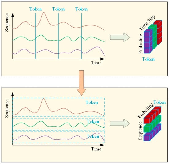
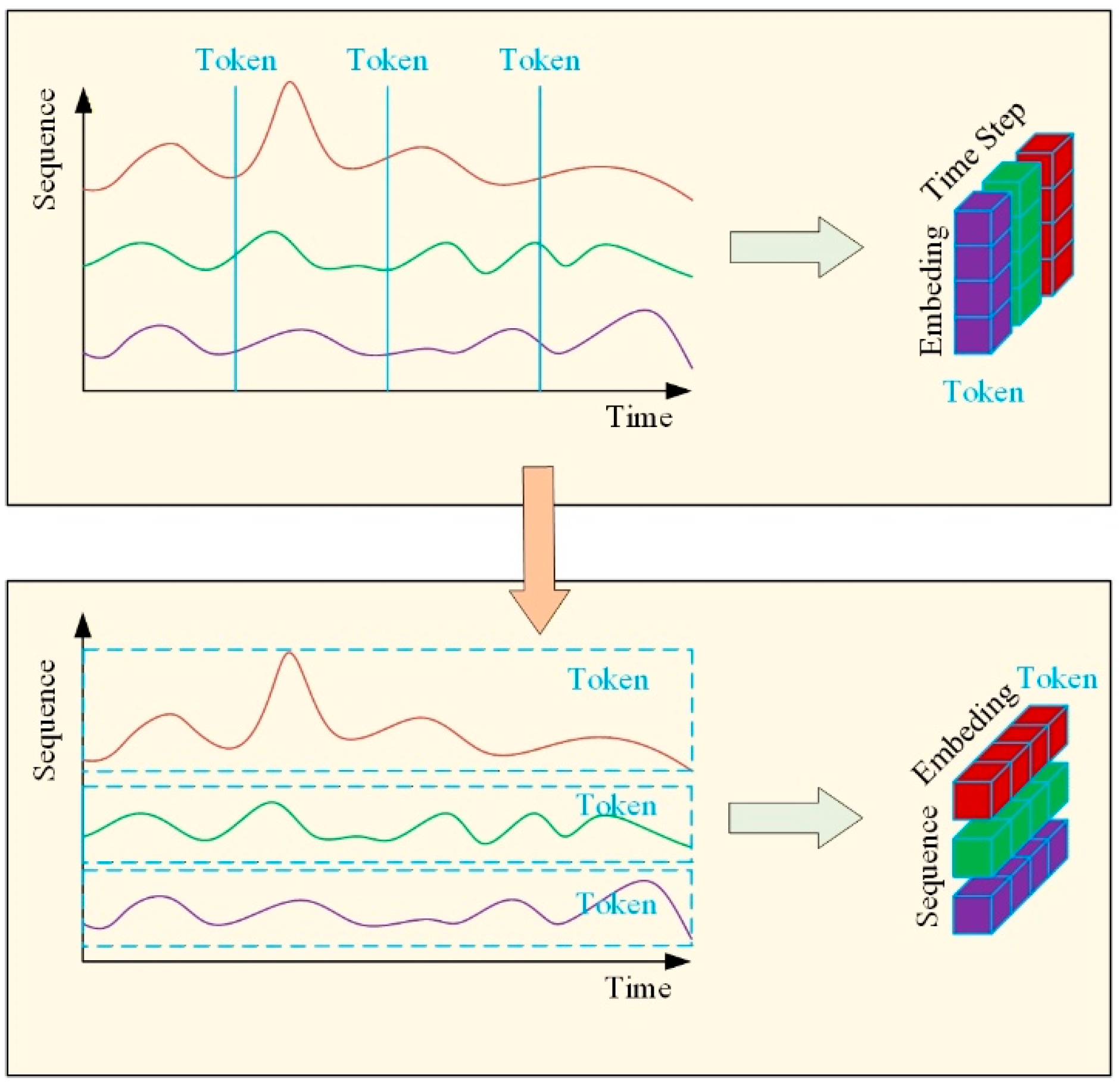
The Informer model incorporates three distinct input embedding strategies: local timestamps, global timestamps, and aligned dimensionality. It embeds each time step into temporal tokens, thereby capturing both localized sequential patterns and hierarchical temporal information. In this work, we transpose the temporal sequence to independently embed variable-specific tokens across the entire sequence. This approach enables the attention mechanism to explicitly model correlations among multiple source sequences. The proposed modification to the input embedding scheme is illustrated in Figure 3.
Figure 3.
Improved Embedding Method for Informer.
2.6.3. Feature Interaction Mechanism
To enhance the encoder’s capability in capturing sequential features, this study introduces a feature interaction mechanism.
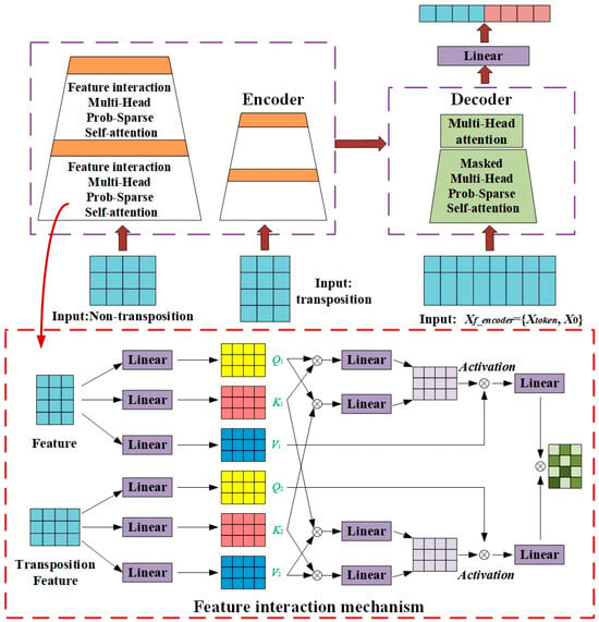
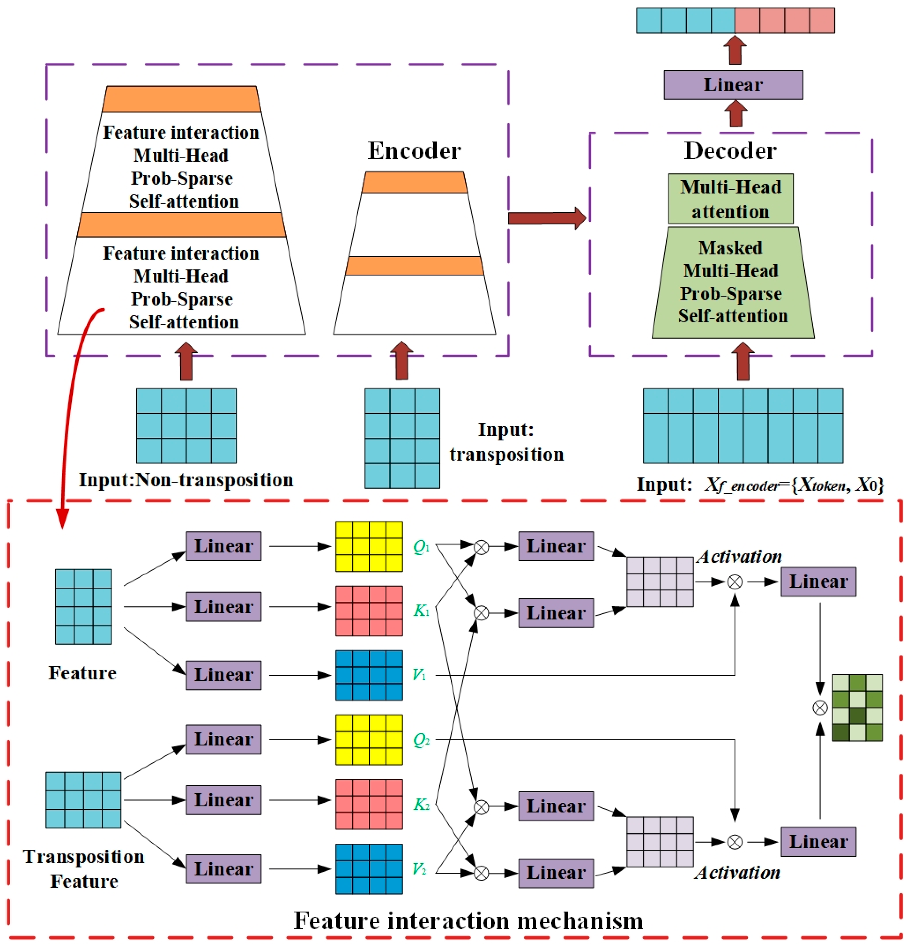
This mechanism adopts a dual-path architecture, where one path takes the original feature map as input while the other takes its transposed version, allowing multi-head attention to be performed on the encoder feature maps from complementary perspectives. In each path, three independent linear layers with GELU activation first generate the attention feature matrices Q, K, and V, respectively. These six attention features are then reshaped into multi-head form. Subsequently, a self-cross similarity computation strategy is applied: dot-product operations are used to obtain both the intra-path self-similarity and the inter-path cross-similarity. The resulting similarity matrices are transformed via separate linear layers with GELU activation, followed by Softmax normalization to derive the multi-head self-attention and cross-attention weights. Finally, the outputs of the two paths are fused through a linear layer to form a comprehensive feature representation. The architecture of the proposed Feature-Interactive Informer (FI-Informer) model is illustrated in Figure 4.
Figure 4.
FI-Informer Model Architecture Diagram.
3. Experimental Data Processing and Analysis
3.1. Data Description and Decomposition Processing
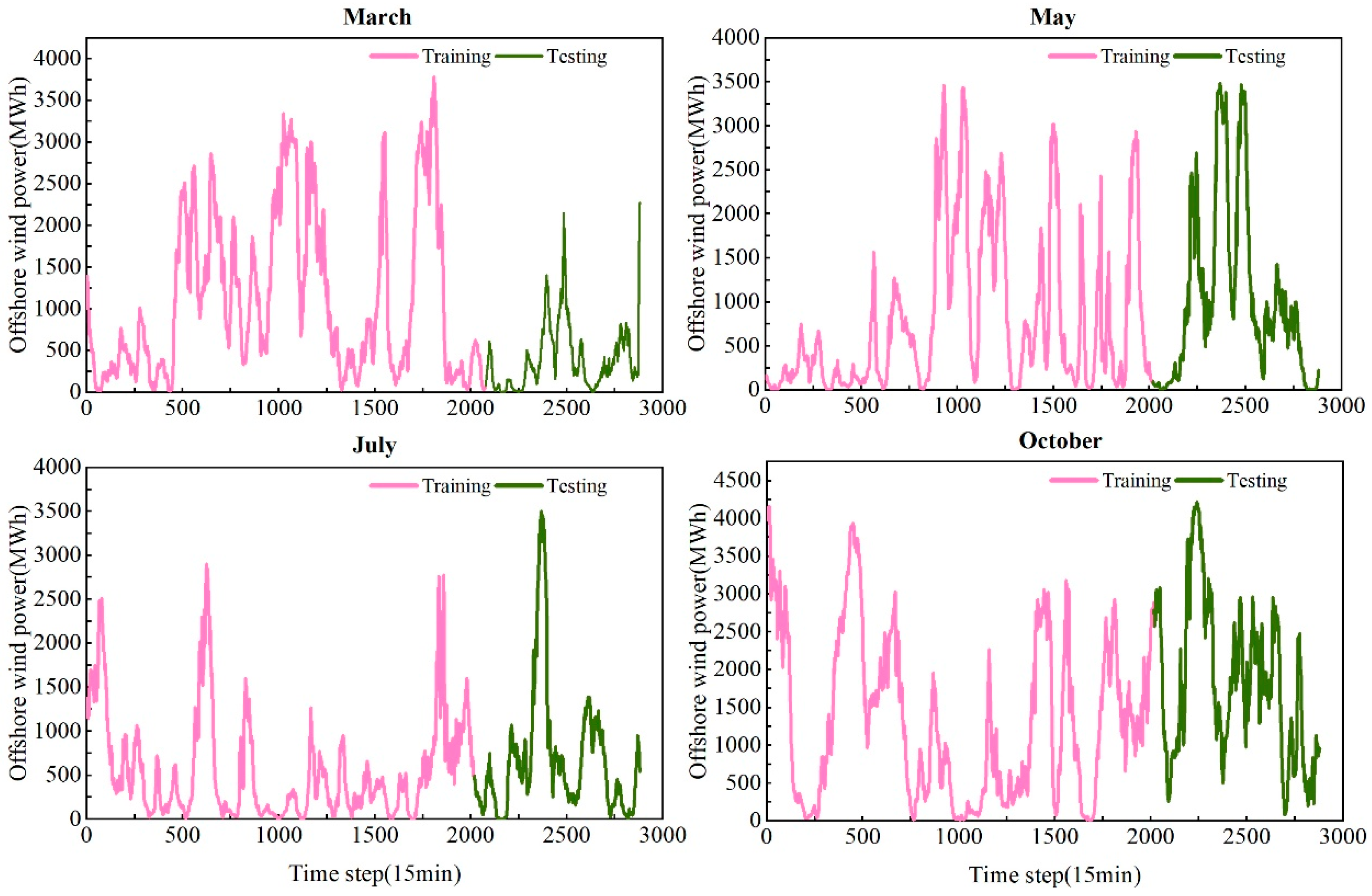
The experimental data employed in this study were collected from a wind farm operated by Elia in Belgium [16]. To account for seasonal variations in wind power generation, power output data from four months (March, May, July, and October 2022) were selected as the original dataset, representing spring, summer, autumn, and winter, respectively. The sampling interval is 15 min, yielding 2880 data points per month. Each monthly dataset is divided into training and testing sets in a 7:3 ratio. Further details are presented in Figure 5 and Table 1. In addition to power measurements, the dataset includes corresponding meteorological features at each sampling point: wind speed (at 10 m and 50 m height), wind direction (at 10 m and 50 m height), atmospheric pressure, temperature, and relative humidity.
Figure 5.
Training data and test data for four months.
Table 1.
Basic information for four sets of monthly datasets.
Figure 5 and Table 1 clearly illustrate the strong stochasticity, pronounced nonlinearity, and high impulsiveness inherent in the offshore wind power data.
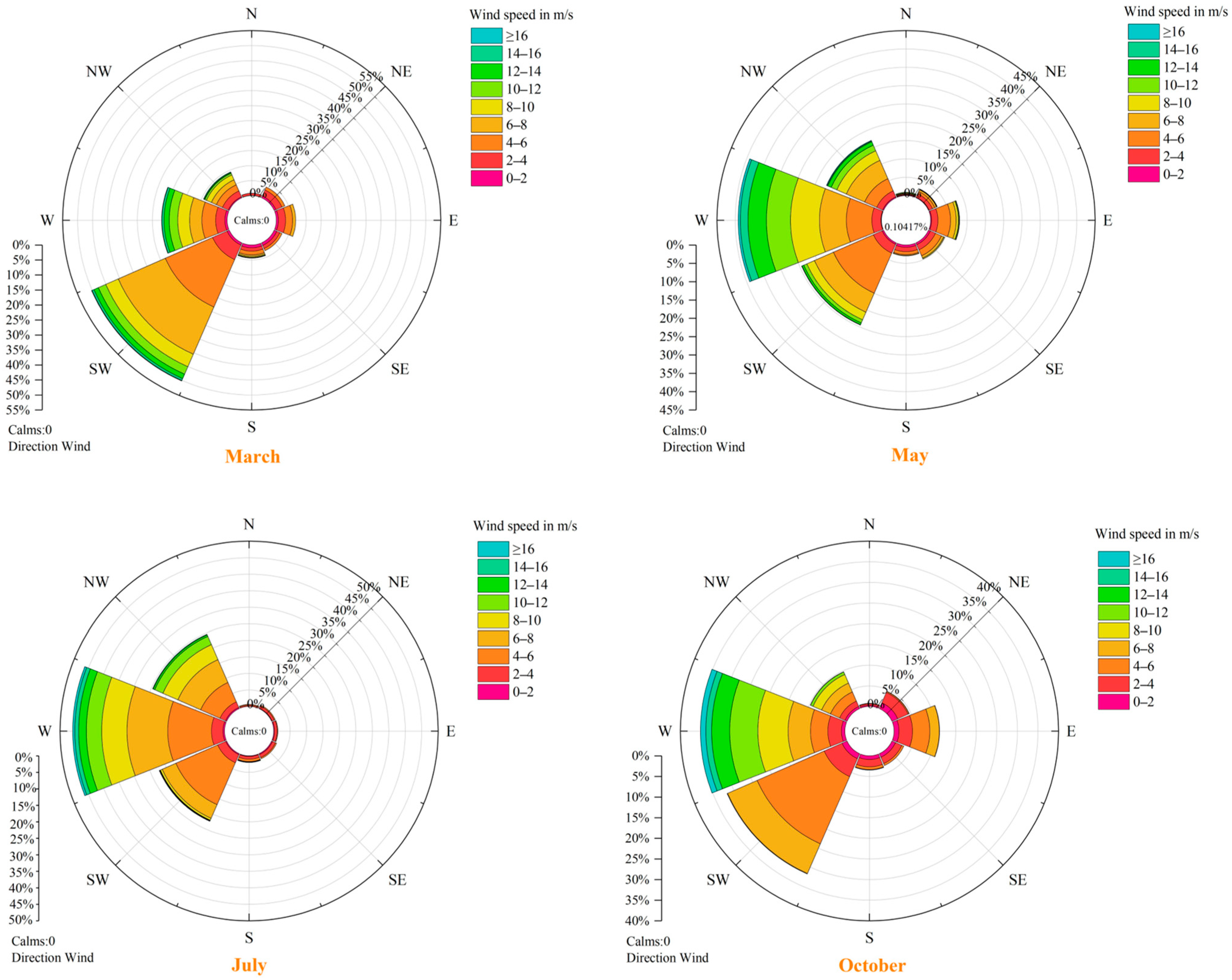
As wind speed and wind direction are critical factors influencing power output, a wind rose diagram (Figure 6) is provided to visually depict the distribution characteristics of these two meteorological variables.
Figure 6.
Wind rose diagram.
The wind rose diagram reveals the coupling relationship between wind speed and direction. Variations in both the magnitude and direction of wind directly influence the power generation characteristics of wind turbines, thereby affecting the overall power output profile.
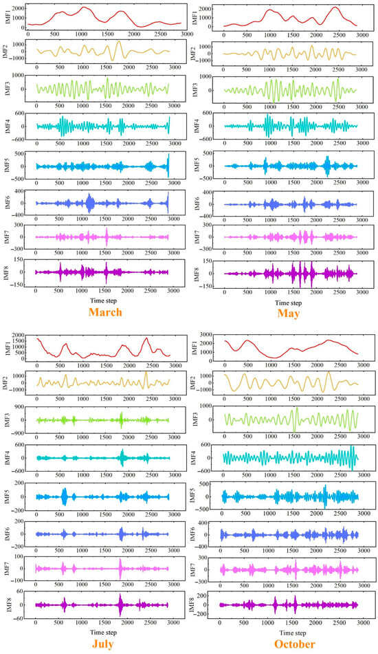
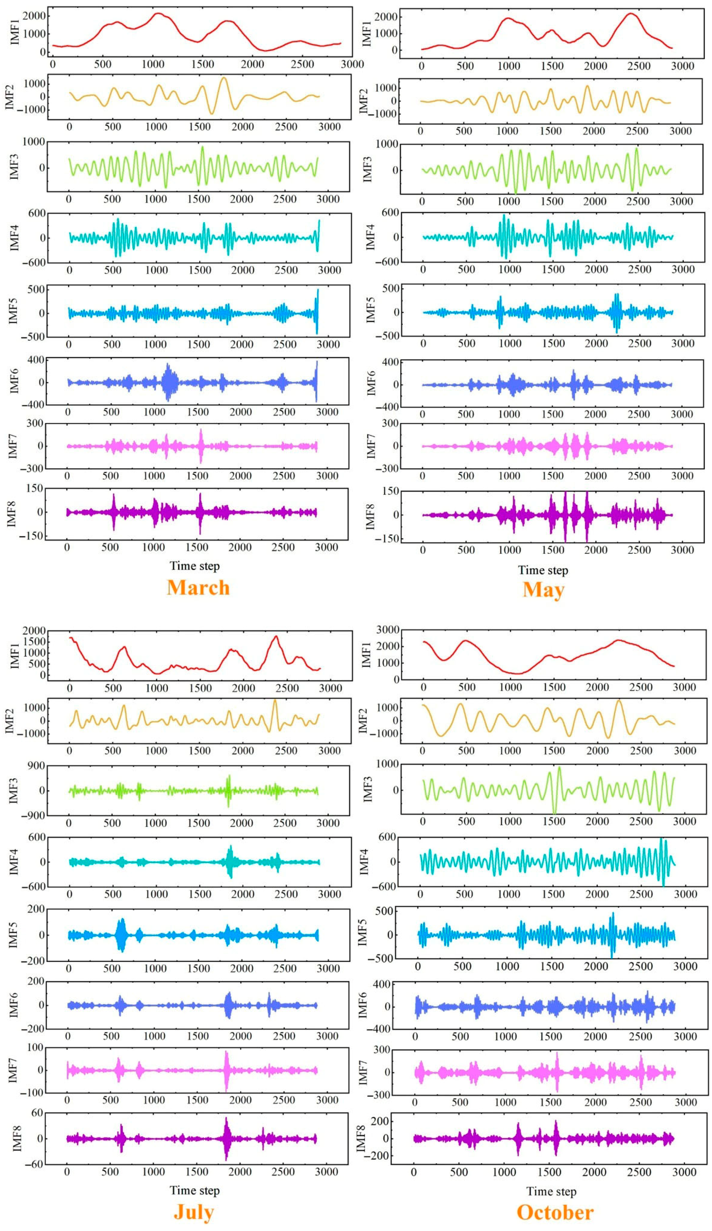
This paper first standardizes all data to the interval [−1, 1]. The operation of scaling the data range to [−1, 1] is performed only during the training phase, then applied to the test phase. Subsequently, the IHBA is applied to optimize the parameters of Variational Mode Decomposition (VMD). The IHBA is configured with a population size of 20 agents, a maximum iteration number of 60, and an acceleration factor of 4.10. The search ranges for the number of decomposition modes and the penalty factor are set to [4, 10] and [250, 2500], respectively. The optimized integer values of these parameters are listed in Table 2, and the decomposition results obtained via the IHBA-tuned VMD are illustrated in Figure 7. The K and α values for each month are listed in Table A2 of the Appendix A. Through extended parameter searches (K = 2–15, α = 200–8000), we found that the optimal VMD parameters varied across months (K = 6–10, α = 600–1500). However, K = 8 and α = 1000 demonstrated robust suboptimal performance throughout the year (differing by only 1.3% from the monthly optimal average). Considering simplicity of engineering implementation, we selected this fixed parameter combination. Future work may explore adaptive parameter tuning strategies to achieve an additional 12% performance improvement.
Table 2.
Integer value of the IHBA-VMD optimization parameter.
Figure 7.
IHBA-VMD Sequence Decomposition Diagram.
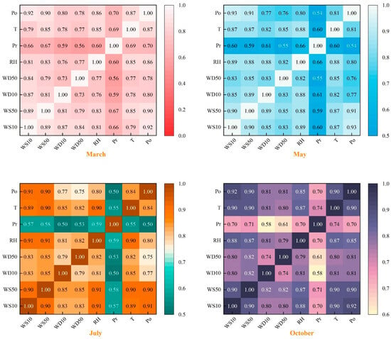
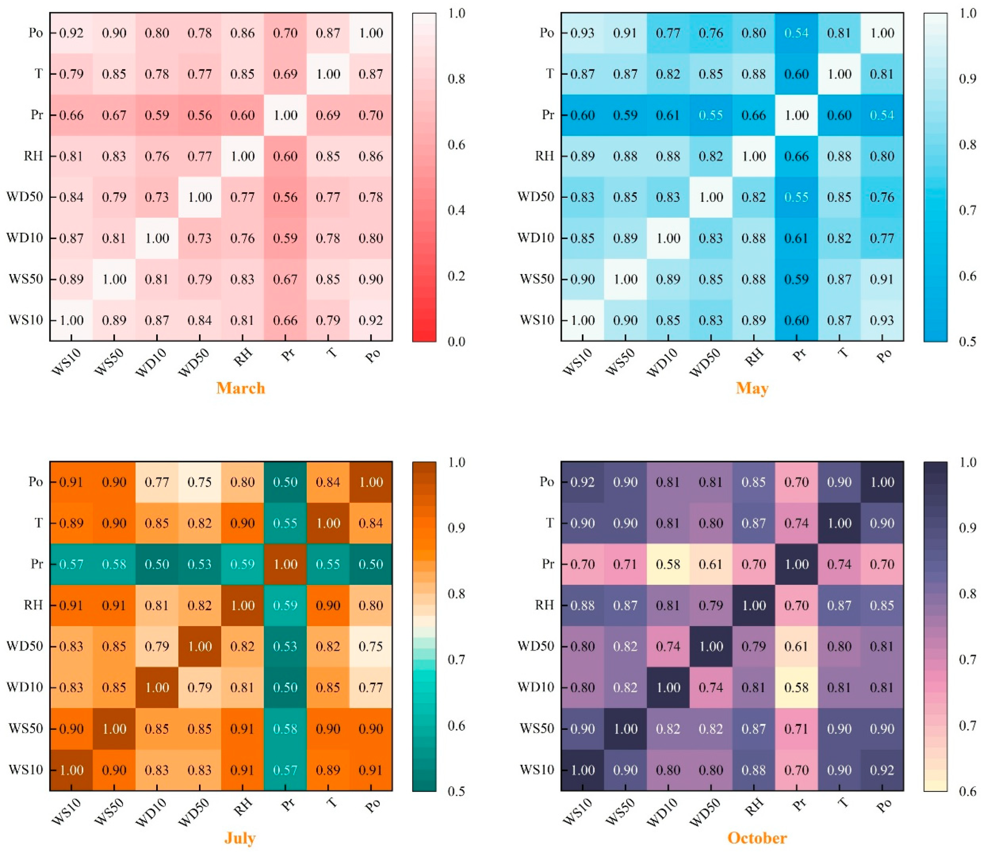
The DE-MIC method provides an effective measure for evaluating the association between offshore meteorological input variables and power output. A higher DE-MIC value indicates a stronger relationship between the variables, while a lower value suggests weaker association. Maintain consistency in threshold selection and features across monthly training data, and set the dynamic grid partitioning threshold for DE-MIC to the top 30% of high-density regions (ranked by maximum information coefficient MIC values). The superiority of the DE-MIC method is demonstrated in Table A3 of the Appendix A.
As shown in Figure 8, heatmaps illustrate the DE-MIC-based correlations between different input features and wind power across the four seasons. The results clearly demonstrate that wind speed (at 10 m and 50 m) and wind direction (at 10 m and 50 m) exhibit the highest influence on power output, with DE-MIC values reaching 0.9 or above in May and July. In July and October, relative humidity and temperature also show DE-MIC values exceeding 0.9, indicating their strong relevance to power generation during these months. Accordingly, these key features are selected as model inputs.
Figure 8.
DE-MIC feature correlation heat map.
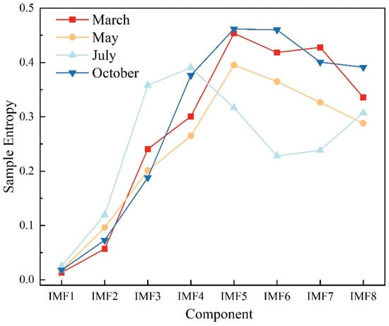
As observed in Figure 7, the VMD optimized with the IHBA effectively alleviates the mode mixing phenomenon. The distributions of Sample Entropy (SE) values for the resulting sub-modes across the four seasons are shown in Figure 9.
Figure 9.
SE value distribution chart in four months.
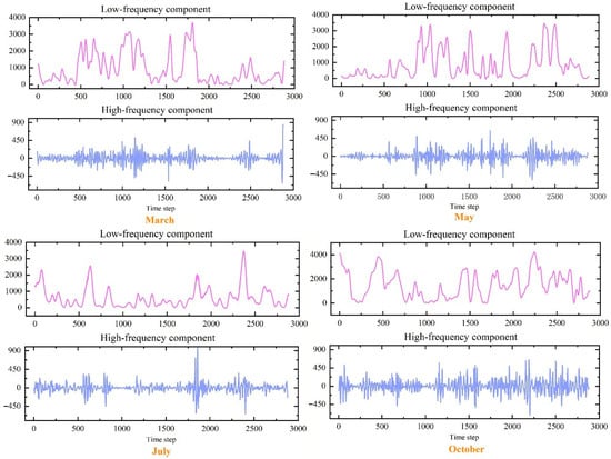
To address the issue of redundant subsequences after decomposition, which would substantially increase computational complexity, this study employs Sample Entropy (SE) to calculate the entropy value of each sub-mode. This step quantitatively characterizes the complexity of the individual modes and allows for their reconstruction into high-frequency and low-frequency components, thereby significantly reducing the overall sequence complexity. The sample entropy parameters were set to m = 2 and r = 0.2*std (a common choice based on the non-stationary characteristics of wind power signals). The median value of the monthly SE was selected as the threshold for reconstruction, with values above the median assigned to the high-frequency group and those below to the low-frequency group. Details are shown in Figure 10. Selecting the median as the threshold is insensitive to outliers, requires no preset parameters or complex calculations, and provides a natural separation point. Compared to fixed thresholds or empirically chosen values, the median is an inherent property of the data itself, eliminating subjectivity. Its sensitivity analysis is presented in Table A4 of the Appendix A. Results indicate that when using the median (P50) as the threshold, performance variations compared to alternative thresholds (P40/P60) remain within ±1%, demonstrating the method’s insensitivity to threshold selection. Schemes with three or more groups did not yield performance improvements but instead increased model complexity.
Figure 10.
SE Modal reconstruction high and low frequency images.
Feeding the obtained high-frequency and low-frequency sequences into their corresponding dedicated models for separate prediction enables effective capture of their distinct temporal characteristics while reducing predictive redundancy, thereby improving the overall performance and robustness of the forecasting framework.
3.2. Evaluation Metrics
To evaluate the prediction accuracy of the model, this paper employs three performance metrics: Root Mean Square Error (RMSE), Mean Absolute Error (MAE), and Mean Absolute Percentage Error (MAPE). All indicators in this article are in MW. Their respective calculation formulas are as follows:
In Equations (32)–(34), denotes the actual observed value of the ith data point, denotes the predicted value of the ith data point, and n denotes the total number of data points.
4. Experimental Results and Analysis
4.1. Ablation Study Analysis
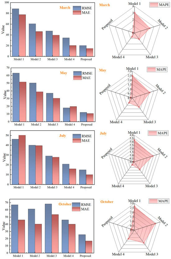
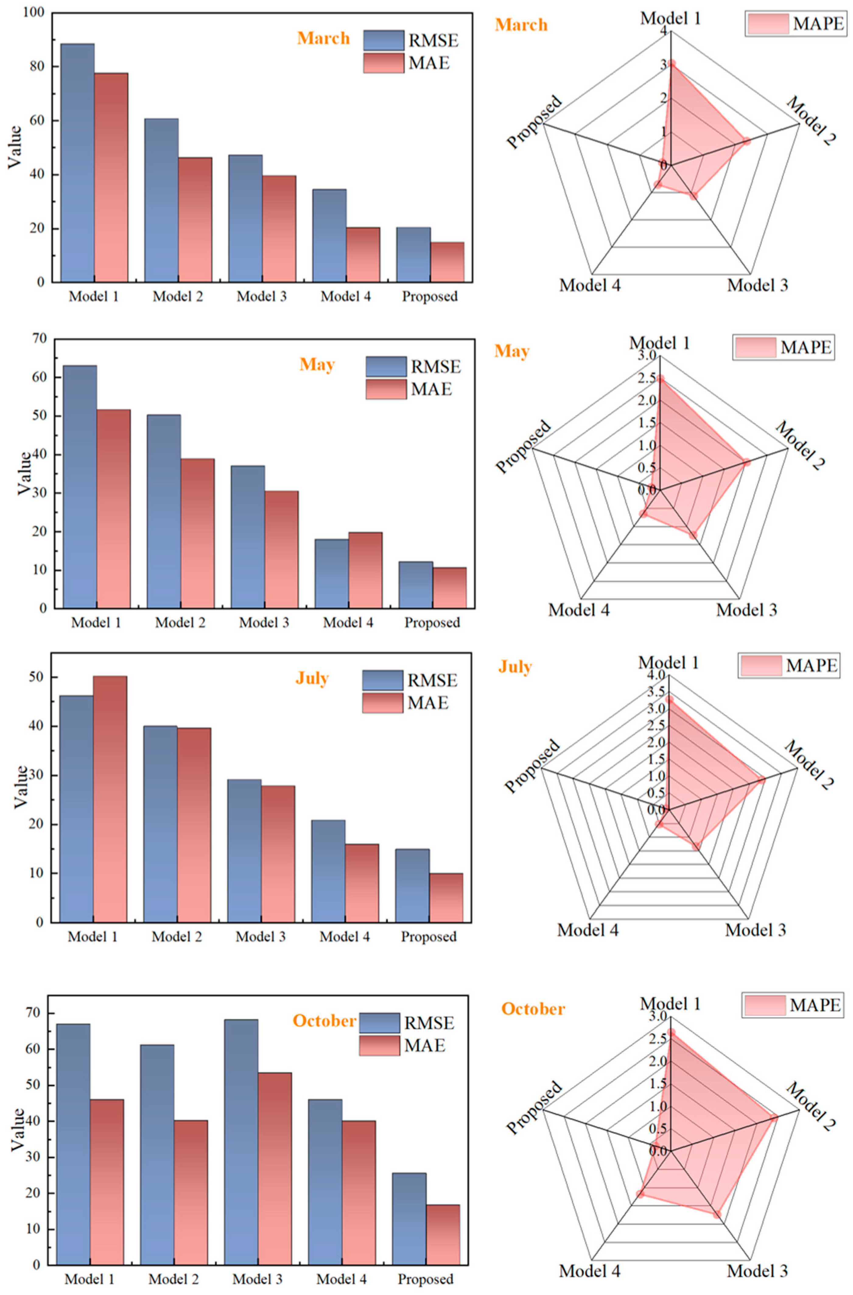
In this study, five distinct models were employed for wind power forecasting, as listed in Table 3. The proposed IHBA-VMD-FI-Informer model was evaluated and compared against these benchmark models. All models perform one-step forecasts with a one-hour lead time (i.e., input data at time t to output power at time t + 1). To ensure fairness, all comparative experiments maintain the same forecast step size and do not employ multi-step rolling forecasts. The comparative performance, measured by Root Mean Square Error (RMSE), Mean Absolute Percentage Error (MAPE), and Mean Absolute Error (MAE), is presented using bar charts and radar diagrams, with the numerical results detailed in Table 4 and visually summarized in Figure 11.
Table 3.
The name of each model.
Table 4.
Four-month evaluation metrics for models.
Figure 11.
RMSE, MAE, and MAPE Plots Across Different Models.
- (1)
- Compared to the baseline Informer model, the proposed hybrid model, which integrates multi-source and multi-scale fusion, demonstrates superior forecasting performance.
- (2)
- For the March dataset, the introduction of the optimization algorithm resulted in a reduction of over 20% in both RMSE and MAE values. Similar reductions in RMSE were observed across other seasons. These results indicate that parameter optimization via the introduced algorithm significantly enhances the model’s predictive capability.
- (3)
- A comparison between the proposed model, Model 3, and Model 4 reveals that incorporating the feature interaction mechanism effectively addresses the Informer model’s limitation in capturing deep dependencies among multi-source data. This is evidenced, for instance, by the RMSE, MAE, and MAPE values of 12.230, 10.662, and 0.211, respectively, achieved in May, thereby validating the efficacy of the proposed feature interaction mechanism.
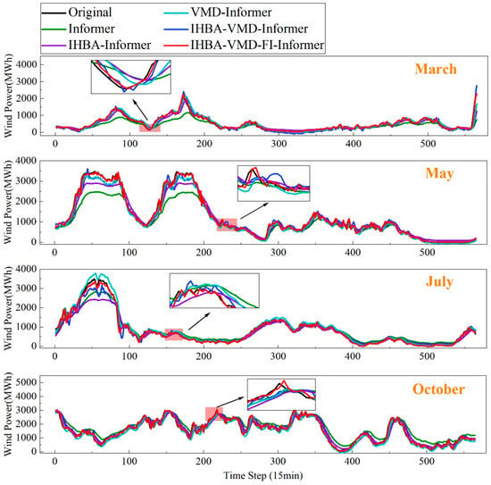
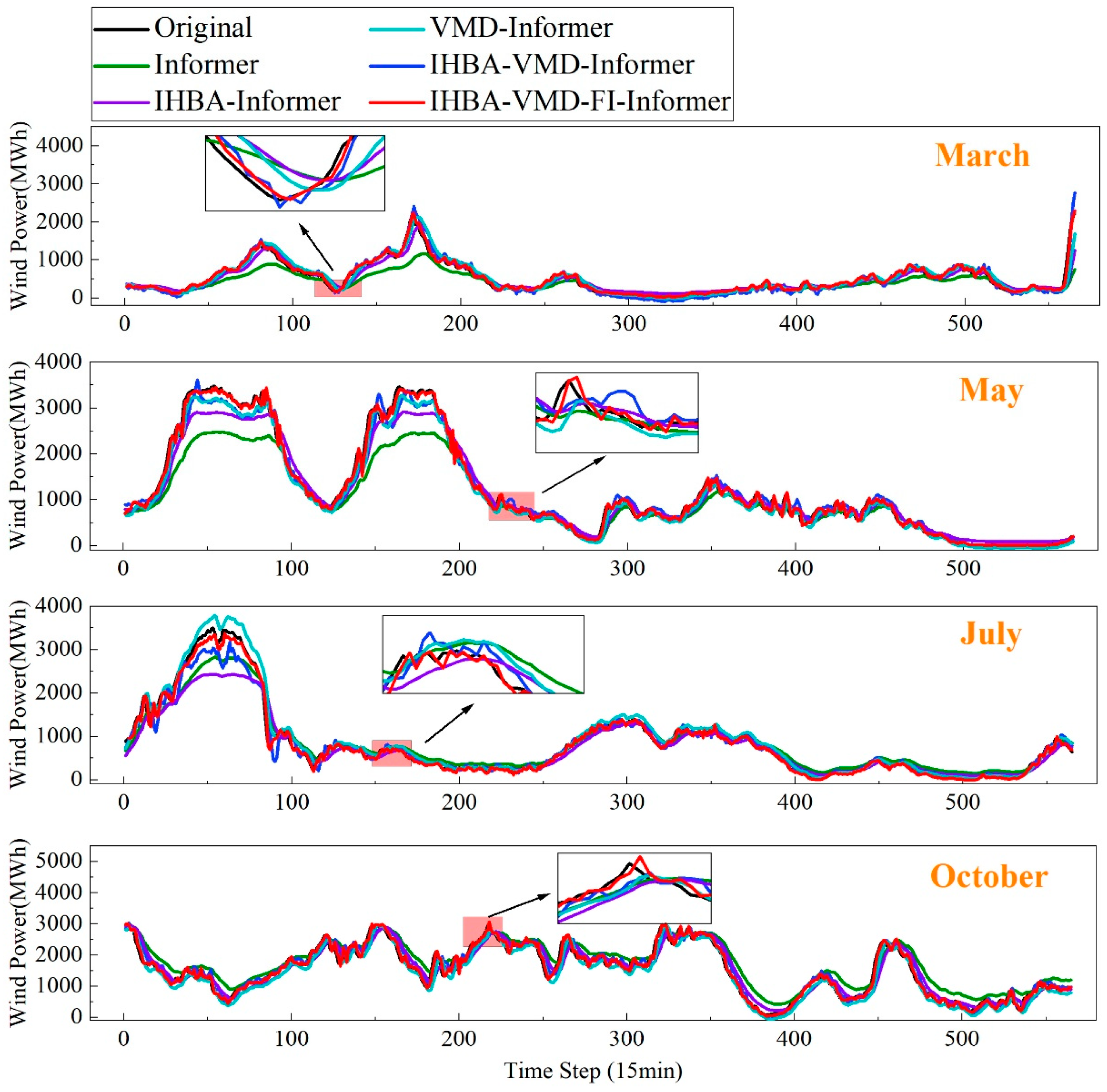
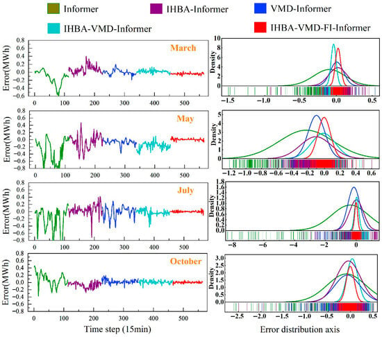
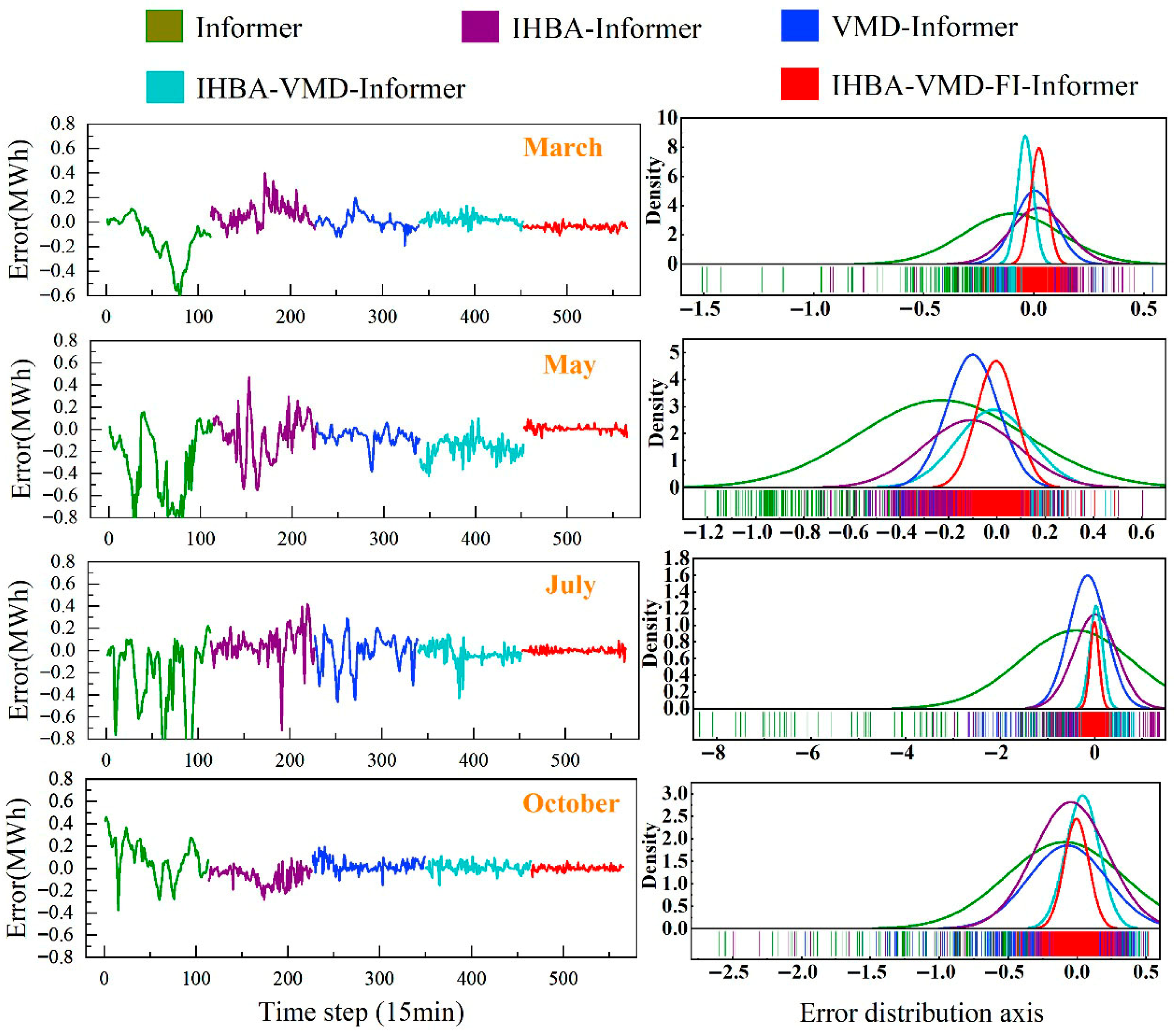
To further validate the accuracy of the proposed model, a comparative analysis of curve fitting from an ablation study is presented in Figure 12. Figure 13 illustrates the relative error plot and the overall error distribution violin plot from the same ablation experiments. Due to the large scale of the underlying data, the errors are normalized to the interval [−1, 1] to facilitate clearer observation and analysis. As indicated in the magnified section of Figure 13, the proposed hybrid model achieves the highest degree of fitting. Figure 13 demonstrates that the proposed model exhibits the narrowest fluctuation range in relative error, with its error distribution being both concentrated and of low magnitude. In summary, the model presented in this study delivers superior performance for offshore wind power forecasting.
Figure 12.
Offshore wind power prediction results.
Figure 13.
Relative error and distribution axis of error.
To demonstrate the statistical robustness of the results, the mean and standard deviation of five runs were calculated for the random model. Statistical significance testing yielded a t-test p-value of 0.0023, which is less than 0.01, indicating a significant difference. This confirms the superiority and stability of the proposed method. Test details are provided in Table A5 of the Appendix A.
4.2. Comparative Experiment on IHBA Intelligent Optimization Algorithms
This subsection presents a comparative evaluation of the low-frequency subsequence forecasting performance among the PSO-Informer, GWO-Informer, and the proposed IHBA-Informer models. Table 5 lists the corresponding evaluation metric values for the low-frequency components across the four months.
Table 5.
Four-month evaluation metrics for different models.
Based on the evaluation metrics presented in Table 5, the IHBA-Informer model demonstrates the best overall performance across the four seasonal datasets. For instance, it achieves the lowest MAPE value of 2.014% for the May dataset compared to the other two models. However, its performance is not optimal for the July and October datasets. This discrepancy may be attributed to the inherent limitation of the Informer architecture in adequately capturing the complex inter-feature relationships within multi-source data.
4.3. Comparative Experiments on Different Data Decomposition Methods
This section compares forecast results using the IHBA-VMD, EMD, and CEEMD data decomposition methods, with specific details presented in Table 6.
Table 6.
Indicators for different data decomposition methods.
As shown in Table 6, the IHBA-VMD method yields significantly lower values for all evaluation metrics. For instance, the MAPE values for the four-month forecasts are 0.290, 0.211, 0.113, and 0.372, respectively. This indicates that the model accuracy achieved using the IHBA-VMD method is higher.
4.4. Comparative Experiments on Different Optimization Algorithms for VMD
Based on a comparison of the benchmark capabilities of intelligent optimization algorithms (see Appendix A Table A6 for details). To validate IHBA’s ability to decompose VMD for optimization, this section compares the iterative decomposition capabilities of PSO-VMD, GWO-VMD, HBA-VMD, and IHBA-VMD. Taking the March decomposition as an example, the results are shown in Table 7.
Table 7.
Evaluation metrics for intelligent algorithm iteration capability.
As shown in Table 7, the optimal parameter solution obtained by the VMD using the improved HBA proposed in this paper exhibits the minimum fitness value and the fewest iterations, indicating that IHBA possesses the strongest optimization capability and that the method improvement is effective.
4.5. Experiments Comparing Widely Used Baseline Models
Most current methods are variants of GRU and LSTM approaches. To validate the superiority of the Informer model as the baseline in this paper, we compared its prediction metrics as shown in Table 8.
Table 8.
Comparison of different baseline models.
As shown in Table 8, the Informer baseline model demonstrates superior performance in this study, while the LSTM and GRU models exhibit relatively weaker capabilities. This may be attributed to the insufficient parallel processing capacity of LSTM and GRU models in multi-scale fusion tasks.
5. Conclusions
This paper proposes a hybrid offshore wind power forecasting model that integrates IHBA, VMD, SE, DE-MIC, and FI-Informer methods for multi-source fusion across high- and low-frequency scales. The performance of the proposed model is comprehensively demonstrated through multi-dimensional analyses, including error metric bar charts, radar charts, relative error plots, and error distribution violin plots. Based on the overall analysis, the following conclusions are drawn:
- (1)
- The model utilizing the IHBA-optimized VMD method demonstrates superior forecasting performance compared to any single constituent model.
- (2)
- In comparison to prediction models based on EMD and CEEMDAN decomposition, the proposed model exhibits better performance. This validates that optimizing decomposition parameters via an improved algorithm effectively enhances the model’s forecasting accuracy.
- (3)
- The phase-space reconstruction of the series into high- and low-frequency dual scales using Sample Entropy (SE), combined with input feature selection via DE-MIC, allows for the full utilization of salient relationships within multi-source data. This reduces redundancy, thereby improving both model efficiency and accuracy.
- (4)
- Introducing a feature interaction mechanism into the Informer model enhances the capture of nonlinear interactions among features, leading to a more precise characterization of the dynamic behavior in offshore wind power systems. Concurrently, it reduces the model’s sensitivity to noise in individual features, further contributing to improved prediction accuracy.
- (5)
- The forecasting results obtained by optimizing the parameters of both VMD and FI-Informer using the IHBA are superior to those achieved without such optimization. This indicates that the HBA enhanced by the three proposed strategies exhibits significantly improved optimization capability.
Author Contributions
Writing—original draft, K.L.; Writing—review & editing, P.H.; Methods, Y.S. All authors have read and agreed to the published version of the manuscript.
Funding
This research was funded by High-level talent introduction project of Zhejiang Institute of Communications, “Research on durability deterioration of reinforced concrete square piles in the marine environment” (Project No. 2024rcxm07).
Data Availability Statement
The data presented in this study are available on request from the first author.
Conflicts of Interest
The authors declare no conflicts of interest.
Appendix A
Table A1.
Comparison of similar methods in the literature with the present method (using March as an example).
Table A2.
Monthly selection of VMD parameters for expandability verification.
Table A3.
Performance comparison of feature selection techniques.
Table A4.
Sensitivity analysis table for median sample entropy.
Table A5.
Model statistical robustness test (using March as an example).
Table A6.
Benchmark capability comparison of intelligent optimization algorithms.
- Detailed Description of the IHBA Optimization Protocol
This study employs an improved honey badger algorithm to jointly optimize key parameters of VMD and FI-Informer. The optimization problem is defined as a 5-dimensional search space, encompassing VMD’s mode count K and penalty parameter α, along with FI-Informer’s attention heads, encoder layers, and feedforward network dimension.
Objective Function: As shown below, the objective function comprises validation RMSE and a model complexity penalty term:
where represents the complexity penalty term and λ = 0.001 serves as the balancing coefficient.
Fitness Calculation Dataset: 70% of data from March, May, July, and October 2022 is used as the training set, with 30% reserved for validation (fitness calculation). Strict chronological partitioning is enforced to prevent information leakage.
Optimization Loop Details: IHBA was configured with a population size of 30 and a maximum of 50 generations. Each fitness evaluation required retraining the entire FI-Informer model from scratch, employing an early stopping mechanism (patience threshold of 15 epochs). The entire optimization process involved 1500 full model training runs, averaging 45 epochs per model, totaling approximately 67,500 forward passes.
References
- Peng, X.; Liu, Z.; Jiang, D. A review of multiphase energy conversion in wind power generation. Renew. Sustain. Energy Rev. 2021, 147, 111172. [Google Scholar] [CrossRef] [Scilit]
- Díaz, H.; Guedes, S.C. Review of the current status, technology and future trends of offshore wind farms. Ocean Eng. 2020, 209, 107381. [Google Scholar] [CrossRef] [Scilit]
- Fernández-Guillamón, A.; Das, K.; Cutululis, N.A.; Molina-García, Á. Offshore wind power integration into future power systems: Overview and trends. J. Mar. Sci. Eng. 2019, 7, 399. [Google Scholar] [CrossRef] [Scilit]
- Zhang, W.; He, Y.; Yang, S. A multi-step probability density prediction model based on Gaussian approximation of quantiles for offshore wind power. Renew. Energy 2023, 202, 992–1011. [Google Scholar] [CrossRef] [Scilit]
- Wang, J.; Hu, J.; Ma, K.; Zhang, Y. A self-adaptive hybrid approach for wind speed forecasting. Renew. Energy 2015, 78, 374–385. [Google Scholar] [CrossRef] [Scilit]
- Wang, H.; Han, S.; Liu, Y.; Yan, J.; Li, L. Sequence transfer correction algorithm for numerical weather prediction wind speed and its application in a wind power forecasting system. Appl. Energy 2019, 237, 110. [Google Scholar] [CrossRef] [Scilit]
- Allen, D.J.; Tomlin, A.S.; Bale, C.S.E.; Skea, A.; Vosper, S.; Gallani, M. A boundary layer scaling technique for estimating near-surface wind energy using numerical weather prediction and wind map data. Appl. Energy 2017, 208, 1246–1257. [Google Scholar] [CrossRef] [Scilit]
- Jung, C.; Taubert, D.; Schindler, D. The temporal variability of global wind energy—Long-term trends and inter-annual variability. Energy Convers. Manag. 2019, 188, 462–472. [Google Scholar] [CrossRef] [Scilit]
- Dong, Y.X.; Ma, S.D.; Zhang, H.C.; Yang, G.H. Wind power prediction based on multi-class autoregressive moving average model with logistic function. J. Mod. Power Syst. Clean Energy 2022, 10, 1184–1193. [Google Scholar] [CrossRef] [Scilit]
- Biswas, A.K.; Ahmed, S.I.; Bankefa, T.; Ranganathan, P.; Salehfar, H. Performance analysis of short and mid-term wind power prediction using ARIMA and hybrid models. In IEEE Power and Energy Conference at Illinois (PECI), Urbana, IL, USA, 1–2 April 2021; IEEE: New York, NY, USA, 2021. [Google Scholar]
- Ding, M.; Zhou, H.; Xie, H.; Wu, W.; Liu, K.; Nakanishi, Y.; Yokoyama, R. A time series model based on hybrid-kernel least-squares support vector machine for short-term wind power forecasting. ISA Trans. 2021, 108, 58–68. [Google Scholar] [CrossRef] [Scilit]
- Ahmad, T.; Zhang, D. A data-driven deep sequence-to-sequence long-short memory method along with a gated recurrent neural network for wind power forecasting. Energy 2022, 239, 122109. [Google Scholar] [CrossRef] [Scilit]
- Xiong, J.; Peng, T.; Tao, Z.; Zhang, C.; Song, S.; Nazir, M.S. A dual-scale deep learning model based on ELM-BiLSTM and improved reptile search algorithm for wind power prediction. Energy 2023, 266, 126419. [Google Scholar] [CrossRef] [Scilit]
- Zhou, H.Y.; Zhang, S.H.; Peng, J.Q.; Zhang, S.; Li, J.; Xiong, H.; Zhang, W. Informer: Beyond efficient transformer for long sequence time-series forecasting. Proc. AAAI Conf. Artif. Intell. 2021, 3512, 11106–11115. [Google Scholar] [CrossRef] [Scilit]
- Wu, H.; Zhang, S.; Xu, Z.; Zhou, J.; Li, T. Informer-Based Wind Power Forecasting for Sustainable Grid Operations: A Case Study in China. IEEE Trans. Smart Grid 2023, 14, 2237–2249. [Google Scholar]
- Chi, D.; Yang, C. Wind power prediction based on WT-BiGRU-attention-TCN model. Front. Energy Res. 2023, 11, 1156007. [Google Scholar] [CrossRef] [Scilit]
- Huang, S.; Yan, C.; Qu, Y.P. Deep learning model-transformer based wind power forecasting approach. Front. Energy Res. 2023, 10, 1055683. [Google Scholar] [CrossRef] [Scilit]
- Gilles, J. Empirical Wavelet Transform. IEEE Trans. Signal Process. 2013, 61, 3999–4010. [Google Scholar] [CrossRef] [Scilit]
- Karasu, S.; Sarac, Z. Classification of Power Quality Disturbances with 2D Discrete Wavelet Transform and Bagged Decision Trees Method. J. Polytech. 2018, 21, 849–855. [Google Scholar]
- Karasu, S.; Sarac, Z. The effects on classifier performance of 2D discrete wavelet transform analysis and whale optimization algorithm for recognition of power quality disturbances. Cogn. Syst. Res. 2022, 75, 1–15. [Google Scholar] [CrossRef] [Scilit]
- Gao, X.; Li, X.; Zhao, B.; Ji, W.; Jing, X.; He, Y. Short-term Electricity Load Forecasting Model based on EMD-GRU with Feature Selection. Energies 2019, 12, 1140. [Google Scholar] [CrossRef] [Scilit]
- Wang, H.; Sun, J.; Wang, W. Photovoltaic power forecasting based on EEMD and a variable-weight combination forecasting model. Sustainability 2018, 108, 2627. [Google Scholar] [CrossRef] [Scilit]
- Sun, H.; Cui, Q.; Wen, J.; Kou, L.; Ke, W. Short-term wind power prediction method based on CEEMDAN-GWO-Bi-LSTM. Energy Rep. 2024, 11, 1487–1502. [Google Scholar] [CrossRef] [Scilit]
- Li, J.; Zhang, S.; Yang, Z. A wind power forecasting method based on optimized decomposition prediction and error correction. Electron. Power Syst. Res. 2022, 208, 107886. [Google Scholar] [CrossRef] [Scilit]
- Guo, X.; Wang, K.; Yao, S.; Fu, G.; Ning, Y. RUL prediction of lithium ion battery based on CEEMDAN-CNN BiLSTM model. Energy Rep. 2023, 9, 1299–1306. [Google Scholar] [CrossRef] [Scilit]
- Tian, Y.; Wang, D.; Zhou, G.; Wang, J.; Zhao, S.; Ni, Y. An Adaptive Hybrid Model for Wind Power Prediction Based on the IVMD-FE-Ad-Informer. Entropy 2023, 25, 647. [Google Scholar] [CrossRef] [Scilit]
- Hashim, F.A.; Houssein, E.H.; Hussain, K.; Mabrouk, M.S.; Al-Atabany, W. Honey Badger Algorithm: New Metaheuristic Algorithm for Solving Optimization Problems. Math. Comput. Simul. 2022, 192, 84–110. [Google Scholar] [CrossRef] [Scilit]
- Layeb, A. Tangent search algorithm for solving optimization problems. Neural Comput. Appl. 2022, 34, 8853–8884. [Google Scholar] [CrossRef] [Scilit]
- Liu, W.; Jiang, Y.; Xu, Y. A Super Fast Algorithm for Estimating Sample Entropy. Entropy 2022, 24, 524. [Google Scholar] [CrossRef] [Scilit]

Disclaimer/Publisher’s Note: The statements, opinions and data contained in all publications are solely those of the individual author(s) and contributor(s) and not of MDPI and/or the editor(s). MDPI and/or the editor(s) disclaim responsibility for any injury to people or property resulting from any ideas, methods, instructions or products referred to in the content. |
© 2026 by the authors. Licensee MDPI, Basel, Switzerland. This article is an open access article distributed under the terms and conditions of the Creative Commons Attribution (CC BY) license.