


Abstract
AC battery systems (ACBSs) based on multilevel converters (MLCs) have gained considerable attention in recent times for the provision of grid services due to high-power (HP) and high-energy (HE) capabilities. In a hybrid ACBS, multiple low-voltage ports provide DC interfaces for battery modules from the same or different chemistries, enabling flexible operation across a wide range of grid services. However, the design complexity increases substantially, due to (i) higher electrothermal coupling between heterogeneous battery modules and power electronic (PE) switches, (ii) grid compliance constraints and (iii) power quality requirements, which often leads to conservative oversizing and, consequently, increased total cost of ownership (TCO). To address these challenges, this paper proposes a co-design optimization framework for the sizing and selection of battery modules, PE components, and MLC architecture. A multi-fidelity modeling approach is presented to co-simulate the battery modules and MLC. The model captures electrochemical behavior, degradation dynamics, and power losses to enable accurate estimation of system-level energy efficiency. The framework then leverages a multi-objective nondominated sorting genetic algorithm (NSGA-II) to perform optimal cell-to-module sizing across different chemistries and MLC levels, while incorporating the inter-module balancing and AC power quality constraints. Comparative simulation studies show that the proposed co-design framework achieves life-cycle TCO reduction of 3.5%, 4.5% and 20% relative to non-hybrid (single chemistry) configurations based on LFP, NMC and LTO chemistries, respectively. The test results validate the effectiveness of the proposed co-design methodology for the optimal design of grid-tied AC battery systems.
1. Introduction
In the context of the European Green Deal, the EU has set a goal to achieve climate neutrality by 2050. Decarbonizing the energy sector, which is responsible for over 75% of the EU’s greenhouse gas emissions, is essential to achieving this target. BESSs are recognized as a key enabler in this transition, offering enhanced reliability, operational flexibility, and integration of variable renewable energy sources into the grid. In recent years, many countries initiated the replacement of gas-fired reserve generators with utility-scale BESS solutions, accelerating the decarbonization of electricity systems.
According to the International Energy Agency (IEA), more than 85 GW of BESS capacity had been deployed globally in the power sector as of 2023 [1]. This capacity is projected to increase fourteen-fold, reaching nearly 1200 GW by 2030. Among the various electrochemical storage technologies, Li-ion batteries currently dominate the market due to their competitive cost (USD 140/kWh in 2023), high gravimetric and volumetric energy densities (265 Wh/kg and 693 Wh/L, respectively), favorable safety characteristics, and long cycle life exceeding 9000 cycles [2]. Forecasts indicate an approximately 40% reduction in battery costs by 2030 relative to 2023 levels, with the TCO projected to decline to around 80 €/kWh in 2030 [2,3].
MLC-based battery systems are increasingly used for grid-connected applications due to their superior power quality, higher conversion efficiency, and improved DC-side fault-ride-through capability over two-level VSIs [4,5,6,7,8,9]. The MLC unifies the bidirectional power conversion and BMS functionality within a single architecture constituting an AC-coupled battery system (ACBS). In the literature [9,10,11,12], a wide range of multiport MLC topologies are reported for ACBSs. Ref. [13] ranks several state-of-the-art configurations using a standardized performance matrix. The symmetric CHB scores better across different matrices and is selected as the baseline architecture.
A major challenge for a grid-connected ACBS is the high TCO, which remains a significant barrier to widespread adoption. Although Li-ion battery cost has decreased by 85% since 2010, it continues to account for more than 50% of the system life-cycle TCO [1,14]. It becomes more significant when ACBSs are required to fulfill both HP and HE requirements. For instance, grid ancillary service FRR demands HP with limited energy requirements, whereas FCR requires both HP and HE capacity to sustain longer activation periods. Conventionally, battery packs based on a single chemistry (mostly LFP) are scaled by extending modules in parallel, often resulting in oversizing, underutilization, and reduced cost-effectiveness [15].
A promising solution is the hybridization approach, which combines the battery modules of different chemistries sized individually for either HP or HE application within a single architecture. Common Li-ion chemistries used for hybridization include LCO, LMO, LFP, NCA, NMC, and LTO. While hybridization enables improved battery utilization of complementary battery characteristics, it introduces significant design complexity due to higher electrothermal coupling between battery modules and PECS. Such coupled systems require multi-objective optimization to minimize TCO without compromising system efficiency, lifetime, or grid-code compliance.
BESS optimization methods reported in the literature aim at either technological objectives (battery degradation, PECS efficiency, lifetime enhancement) or economic objectives (TCO, operating profits). In [16,17], BESS sizing for microgrids is formulated as a nonlinear optimization problem, balancing investment cost and lifetime using the BPSO method. GA is reported in [18] to optimize BESS capacity in co-located photovoltaic plants for dispatchable output smoothing. Multi-objective approaches based on NSGA-II are adopted in [18] to optimize the BESS size in co-located wind and photovoltaic plants. The use case focuses on mitigating power fluctuations from both plants and delivering a stable output. To minimize battery degradation and idle energy consumption while maximizing annual net profit, NSGA-II is utilized in [19,20].
In [15] a TCO optimization is extended to include (two-level VSI-based) PECS sizing for a grid-connected hybrid BESS using a combination of HP and HE battery packs by selecting a global solution from multiple Pareto fronts. Refs. [21,22] aim at control-oriented BESS sizing by integrating subcomponents and advanced control strategies. Ref. [23] summarizes the BESS optimization methods, including GA, NSGA-II, simulated annealing, BPSO and ant colony optimization.
Despite extensive literature, ACBS optimization remains largely unaddressed. Existing sizing methods [15] are limited to two-level PECS, where AC and DC sides are effectively decoupled, and battery modules within a single pack are assumed to share energy uniformly. These assumptions are no longer valid for ACBSs.
First, AC-side power quality is governed not only by the cumulative pack voltage but also by the voltage of individual battery modules [16,17]. Second, the energy exchanged by each battery module is a function of its port position within the MLC stack, leading to non-uniform energy flow across the pack due to asymmetrical energy distribution among the ports [5]. Furthermore, hybridization introduces an additional layer of constraints, as each ACBS port can integrate battery modules of different capacities and chemistries.
In view of these constraints, this paper presents a multi-fidelity model and an interoperable COF for co-simulation and techno-economic sizing of hybrid ACBSs. Using a real grid FCR service as a mission profile, the proposed framework simultaneously targets three objectives: (a) improving energy efficiency, (b) maximizing operational lifetime, and (c) minimizing the life-cycle TCO, while ensuring compliance with the grid code requirements.
In this study, cells from three different chemistries, LFP, NMC and LTO, are used to construct HP and HE battery modules interfaced with a MLC realized using SiC MOSFETs. The framework explores the combined design space of battery chemistry selection, module sizing (voltage, capacity) via a combination of series and parallel cells, DC port allocation, and number of MLC voltage level selection to identify an optimal solution. The main contributions of this paper are highlighted as follows.
- (i)
- A multi-fidelity electrothermal model is developed for battery modules from different chemistries and MLCs, enabling real-time co-simulation of hybrid ACBSs and estimation of power losses under various mission profiles.
- (ii)
- A TCO model is formulated to evaluate life-cycle cost by accounting for battery degradation, replacement, and energy losses.
- (iii)
- A co-design optimization framework (COF) is developed to perform (i) cross-chemistry cell-to-module sizing, (ii) module balancing, (iii) allocation of HP and HE chemistry on the DC ports within a single architecture and (iv) MLC voltage level selection while satisfying the grid constraints.
The remainder of this paper is structured as follows: Section 2 presents the system overview and the mission profile selection for the proposed framework. Section 3 highlights the co-design challenges for the hybrid ACBS and builds the problem foundation. Section 4 provides a high-level flow chart and an overview of the methodological stages. Section 5 details the electrothermal modeling of the PECS and battery modules. It also introduces the life-cycle TCO modeling for the ACBS. Section 6 describes the implementation of the COF, including the definition of design variables, system constraints, and objective functions. Section 7 presents the optimal solutions derived from the different Pareto fronts and the corresponding sensitivity analysis. It also highlights the FEC evolution of the various battery modules in the global optimal configuration. Section 8 concludes the paper while Section 9 outlines the study limitations and directions for future work.
2. Hybrid ACBS Description
2.1. System Overview
Figure 1 depicts the schematic of the hybrid ACBS considered for the proposed COF. On the DC side, the battery pack consists of a combination of HP and HE battery modules based on three Li-ion chemistries: LFP, NMC and LTO.
Figure 1.
Schematic illustration of the hybrid AC battery system.
On the AC side, a cascaded full-bridge-based MLC realizes the multiport PECS configuration. Each battery module is connected to the DC port of the PECS via a pre-charge resistor and two interfacing relays constituting a submodule.
Figure 2 illustrates the per-phase implementation of a hybrid ACBS where battery modules are cascaded in series using low-frequency PE switches in the MLC. The output AC voltage and number of levels can be expressed as follows [18]:
where represents the maximum value of the AC voltage, is the battery module voltage and is the maximum number of full bridges connected in series. The MLC output voltage consists of levels in total, with magnitudes in positive and [negative] half cycles.
Figure 2.
Per-phase illustration of ACBS.
Each submodule comprises a full bridge circuit with four switches ( and is governed by an independent modulation index where . The choice of determines connectivity or bypassing of a battery module in the MLC circuit and therefore regulates the value of the instantaneous MLC voltage by controlling the number of battery modules cascaded at each step.
2.2. Mission Profile
A nominal power rating of , with a 95% design DoD ( is considered for the hybrid ACBS to provide symmetric FCR at to the Belgian TSO. A four-hour real-field grid FCR profile is adopted as a mission profile for the hybrid ACBS [19]. Historical frequency measurements over the calendar year 2024 are analyzed to capture the worst-case mission profile.
The worst-case operating scenario is extracted using a sliding-window algorithm applied to the year-long frequency dataset. For each four-hour window, the measured frequency deviations are converted into a proportional power response according to the TSO specifications [24] and normalized to the rated system power of 100 kW. Two severity metrics are evaluated for each window: (i) the maximum root-mean-square (RMS) current over the window, representing peak power demand, and (ii) the cumulative charging/discharging energy throughput, representing sustained energy exchange and deep DoDs.
The selected mission profile corresponds to the window that simultaneously exhibits a high score on both matrices, thereby constituting the most demanding operating condition for hybrid HP/HE sizing. These frequency deviations are then re-synthesized into a proportional power response normalized to the peak system power of 100 kW.
Figure 3a,b illustrates the year-long frequency measurements, while Figure 3c shows the selected four-hour worst-case window (April 2025, 08:00–12:00), which ranks highest according to the combined power–energy severity criteria. Figure 3d depicts the ENTSO-E power–frequency characteristic used to synthesize the power profile, with a temporal resolution of 10 s, resulting in 1440 samples stored as a *.mat mission profile within the COF framework.
Figure 3.
Belgian grid FCR mission profile overview for the proposed COF: (a) Frequency variation during the first half of 2024.; (b) Frequency variation during the second half 2024; (c) a representative four hour window extracted from the year long profile; and (d) the corresponding active power profile applied to ACBS.
During the FCR provision, the hybrid ACBS is assumed to operate at unity power factor, in line with the TSO specifications [24], which mandates the active power response under frequency deviations. Reactive power injection and voltage support are governed by separate grid-connection requirements (RFG) under the ENTSO-E and are therefore considered outside the scope of this study.
Under the 95% and C-rate of 0.5, the ACBS nominal energy is calculated as 210 kWh. For lifetime assessment and battery cycle calculations, an effective DoD is employed by applying a safety factor to in order to account for the operational margins (further explained in Section 5.3).
3. Co-Design Challenges and Problem Foundation
In MLC-based systems, level-shifted (LS) PWM is widely adopted due to its favorable efficiency characteristics and lower harmonic distortion [20,21]. In LS-PWM, a single sinusoidal modulating signal generated by the high-level current controller is compared against multiple carrier signals that are vertically shifted within the modulation space [25,26,27,28]. Each carrier signal corresponds to one full-bridge (FB) submodule, and the vertical position of the carrier determines the insertion interval of the associated battery module within each grid cycle [21].
Referring to Figure 2, the participation of the battery modules in the AC voltage building process is based on the relative position of their carrier signals. Due to discrete level shifting, each battery module is inserted into the MLC stack for a different cumulative duration during one fundamental AC voltage period. This duration, denoted as the switch-in time determines the energy exchanged between the grid and battery module as expressed below.
where denotes the nominal voltage of the battery module, is the RMS grid current, represents the absolute energy of the submodule, is the time period of the fundamental AC voltage and is the cumulative insertion time of the battery module within one grid cycle.
is a function of the carrier position, and for cascaded submodules, it can be expressed as follows.
where denotes the indicator function. Simplifying Equations (3) and (4) yields the monotonic relationship
To quantitatively characterize the imbalance, the normalized energy contribution of each submodule is defined as follows
Equation (6) provides a quantitative metric to compare module-level energy utilization and to compute normalized ratios ( for different MLC voltage levels. It also highlights how the variation in can lead to asymmetric energy exchange between the AC grid and battery modules.
Figure 4a illustrates the resulting energy mapping for different MLC configurations, where the number of AC voltage levels increases from nine to seventeen, and the number of cascaded submodules increases from four to eight. Figure 4b depicts the stepped AC voltage waveform for a nine-level configuration. The corresponding normalized energy ratios demonstrate that submodules located in the lower region of the modulation space experience significantly higher energy throughput.
Figure 4.
Energy mapping overview of each ACBS port for different MLC levels: (a) tabulated output voltage and energy values for MLC levels ranging from 9 to 17; and (b) illustrative case of a nine level MLC highlighting the asymmetric energy contribution for four battery modules.
Looking at Figure 4b, the battery modules located in the lower region of the modulation space get a higher switch-in time compared to those positioned in the upper region. Consequently, during each cycle of the AC voltage, the lower-positioned battery modules contribute more significantly to the AC voltage building process.
For a nine-level MLC, battery module-1 supplies two times higher energy than battery module-3 during the grid injection mode and therefore discharges twice as fast as battery module-3. Conversely, during the offtake mode, battery module-1 charges twice as fast as battery module-3, leading to an energy imbalance after a few cycles.
Conventionally, a single battery pack has identically sized modules, and modulation strategies are adjusted to mitigate this imbalance by repositioning the SMs within the modulation space every few cycles [29]. In these techniques, SoC and are used as feedback signals to reorder the stack [20,21]. However, the frequent reordering introduces nonlinear loading, increases switching transients, leading to higher switching losses (>5%) [29,30,31,32,33]. In addition, HP modules are pushed down the stack due to temporarily low , further exacerbating inefficiencies and THD.
In contrast, by employing a hybrid configuration, the proposed COF intentionally exploits the deterministic energy mapping imposed by LS-PWM. HE battery modules are sized with higher nominal capacities and are assigned to lower positions in the stack, while HP modules with smaller nominal capacities are assigned to the upper positions.
The correctly sized modules improve the MLC dynamic response and mitigate the drawbacks of conventional reordering every few cycles. The SoC of different modules increases/decreases linearly as each module undergoes the same FEC for a given mission profile, leading to a minimal imbalance.
4. Methodology
Figure 5 presents the high-level flow chart of the proposed modeling strategy, which is divided into three stages.
Figure 5.
High-level flow chart for the modeling strategy.
In the first stage, the system topology is selected (as described in the preceding subsections), resulting in a CHB-based architecture and battery modules from LFP, NMC and LTO chemistry. FCR-based grid service is selected as the mission profile, which defines the nominal energy capacity and power rating of the hybrid ACBS.
In the second stage, detailed electrothermal battery models and high-fidelity PECS models are developed to co-simulate both subsystems and quantify power losses for the ACBS. However, executing the high-fidelity model over the four-hour mission horizon within the COF is computationally intensive and time-consuming, as it requires a large number of iterative simulations.
To improve the execution time, this paper adopts a loss-mapping approach. In this approach, relevant quantities are precomputed and stored as lookup tables, enabling rapid processing during system-level simulations. These lookup tables are then embedded in low-fidelity (Lofi) models used in the third stage for system-level simulations within the CO. Energy mapping is then performed for each ACBS port ( ranging from nine to seventeen), considering a LS-PWM-based modulation strategy.
The PECS Lofi model incorporates three 2D lookup tables: (i) Active power losses, (ii) voltage and current THD and (iii) MLC voltage and module RMS current, all as a 2D function of MLC levels and input power. Similarly, the Lo-fi model for the battery module consists of 2D lookup tables relating (i) battery power losses and (ii) module voltage, both as a function of . Stage 2 evaluates the cumulative energy efficiency of the battery and the PECS over the four-hour mission profile, while Stage 3 integrates the results into the COF framework to compute TCO, system efficiency, and lifetime metrics. The individual stages of the proposed modeling framework are detailed in the next subsections.
5. System Modeling for COF
5.1. Battery Model (Cell to Module)
The electrical behavior of a Li-ion battery cell is represented using a second-order electrothermal model that integrates both electrical and thermal dynamics, as reflected in Figure 6 [34]. It combines a constant RC-based electrical equivalent circuit with a thermal model. The circuit contains a DC voltage source that captures the cell OCV variations with respect to SoC in series with a variable resistor that accounts for the cell’s internal resistance in steady state. The parallel branches are connected in series to account for the cell’s dynamic voltage response, as illustrated in Figure 6. Each RC block is characterized by a time constant that corresponds to a specific dynamic behavior under varying current profiles [27,28]. The OCV and internal resistance parameters are derived through the open-source experimental data reported in [35,36,37,38], while the additional cell parameters are extracted from the CCT database available in [36].
Figure 6.
Second order equivalent circuit based model of battery cell.
Figure 7 illustrates the family of OCV and internal resistance curves for LFP, NMC and LTO chemistries at an ambient temperature of . The curves are obtained for the full range of SoC and C-rate and respectively. The family of curves highlights the nonlinear dependence of cell OCV and internal impedance on operational C-rate and SoC. As shown in Figure 7, this effect is particularly significant for LFP chemistry compared to NMC and LTO. The internal resistance parameters overlap during the low SoC range for all C-rates . However, beyond decreases, whereas increases significantly.
Figure 7.
OCV and impedance of LFP, NMC and LTO cells for different C rates and SoC values.
To account for these nonlinearities, a lookup-table-based representation is used, where OCV and internal impedance are defined as two-dimensional matrices indexed by SoC and C-rate. Table 1 presents the overview of the LFP, NMC and LTO cell specifications considered for the COF. Based on this dataset, a parameterized cell-to-module model is developed for each of the three chemistries.
Table 1.
Cell specifications of three chemistries considered for the COF.
The model aggregates electrothermal cell behavior to the module level by accounting for the series () and parallel () cell connections. Using ambient temperature ( andmodule current profile () as inputs, it first calculates the actual C-rate and SoC per chemistry. The terminal voltage is then computed using two-dimensional spline interpolation of OCV and internal resistance maps as functions of SoC and C-rates, without fitting to time-domain experimental current profiles. The model evaluates ohmic and entropic heat generation, cooling requirements under forced-air conditions, and the resulting thermal equilibrium. This formulation enables consistent estimation of module-level losses, including cooling power demand, and charge/discharge efficiency under realistic mission profiles.
From the model inputs, the cell-to-module voltage, heat generation, losses and efficiency can be calculated as follows.
where represents the terminal voltage of the battery module. [] is the instantaneous C-rate calculated per individual cell using the nominal value from Table 1. denotes the module OCV. accounts for the heat generation inside the cell due to ohmic losses. denotes the cell current. represents the initial SoC of the battery module at the beginning of the mission profile. [W] denotes the entropic/reversible heat generation inside the module calculated using the Bernardi Equation (14). [] is the module plate’s convective heat-transfer coefficient. For forced air cooling, is considered in the range 30 to 80. S [ is the module plate’s area exposed to forced air flow. The variables and denote the module mass [kg] and specific heat capacity [] respectively. provides the total internal heat of the module, while provides the heat evacuated out of the module.
Under thermal equilibrium conditions, . Therefore, Equations (15) and (16) can be equated considering the peak value of during the four-hour window. By enforcing the desired temperature of , a fixed value is obtained for the product from where can be calculated. Finally, the cooling power () is calculated considering the coefficient of performance (COP) of 15 [38].
where is the module thermal time constant governing temperature response under convective cooling conditions and is distinct from the RC time constants of the electrical circuit in Figure 5. The instantaneous power losses of the battery module and AC battery pack can be expressed as follows:
where is the sum of the module internal losses ( and the required cooling power. denotes the total losses of the AC battery pack. and represent the charging and discharging efficiency of the AC battery pack respectively.
Compared to discharging efficiency (92–95%), the battery module exhibits slightly better efficiency (96–98%) during the charging process. The difference is mainly due to higher values of resulting in smaller ohmic loss during the charging process [39,40,41]. and represent the output power of the module during charging and discharging respectively.
The battery model outputs comprise (i) , (ii) (a vector of signals) (iii) (iv) module active power and (v) auxiliary power requirement (.
5.2. PECS
The PECS interface in the hybrid ACBS consists of a MLC architecture, where multiple FBs are cascaded in series to synthesize the desired AC voltage. To obtain PECS power losses, a high-fidelity switching model for the CHB-MLC is developed in C and parameterized using the SiC MOSFET datasheet specifications.
The model is compiled via the MATLAB R2022b MEX interface and integrated into the SIMULINK environment. Figure 8 depicts the structure of the coupled battery module and PECS switching model. For clarity, both the models are distinguished using separate colors.
Figure 8.
Switching model and interconnecting signals for PECS and battery modules comprising (a) MLC switching model, (b) detailed battery module model, (c) LS-PWM-based modulator for generating gating signals and (d) Lofi models comprising lookup tables to store 2D maps of detailed loss models.
The model accepts parameters and vectorized inputs through the high-level block in SIMULINK, which are then passed to the lower-level C-based FB models. The input vector consists of (i) , (ii) (a vector of signals obtained from the battery model), (iii) instantaneous AC side current (), (iv) gating signals (, (v) , (v) and (vi) the MOSFET parameters. The input vector values and parameters used are summarized in Table 2.
Table 2.
Parameters and values for PECS model (P: parameter, V: run-time value).
The switching model is executed at a single-phase peak power of selected from the mission profile in Figure 3. To capture the switching dynamics, the simulation step time of is considered. The RMS value of the inductor current is extracted from the instantaneous waveform and subsequently used to calculate the MOSFET power losses according to Equations (22)–(26).
The model outputs include (i) , (ii) (a vector of signals reflecting instantaneous battery module current waveforms, (iii) (iv) (v) active power () and (vi) power losses (.
5.2.1. Modulation Scheme
The switching model integrates LS-PWM for gate signal generation, as illustrated in the modulation block. The modulator receives reference modulating signal, switching frequency, and the number of MLC levels as inputs. Based on the specific number of levels, the corresponding carrier waveforms () are generated, vertically shifted and linearly arranged within the modulation space. A comparison between the modulating reference and set of carrier waveforms produces the gate signals ( which serve as inputs to the switching model.
5.2.2. Loss Modeling
Table 3 presents the operational modes of a single SM (depicted in Figure 2) as a function of the modulation index. Modes 1–2, {3, 4} represent charging, discharging and {bypassing} of each battery module respectively. For CHB topology, modes 5 and 6 (highlighted in Table 3) are not used as a negative value of the modulation index (reverse cascading) is not applicable for LS-PWM.
Table 3.
Operational modes of SM as a function of modulation index.
The FB losses include the MOSFET losses (conduction and switching) and gate driver losses as expressed below:
where and denote the MOSFET conduction and switching losses respectively. is the drain to source resistance of MOSFET during the ON state. It is the function of junction temperature and remains the dominant source of loss due to low switching frequency (1.1 kHz), as illustrated in Figure 9c. and are turn-on and turn-off delays respectively. denotes the gate driver losses and is ignored as it constitutes less than 0.1% to the total PECS losses ( denotes switching losses and is estimated from the turn-on energy and turn-off energy as per Equation (21).
Figure 9.
Output waveforms of PECS switching model under , P = 33 kW, (a) instantaneous voltage (V) and current (A), (b) instantaneous battery module currents SM1–SM6 and (c) conduction and switching losses.
Figure 9a and Figure 10a illustrate the output waveforms (instantaneous MLC voltage and current) of the PECS switching model for values of thirteen and twenty-one respectively. For , there are six () output battery module current vectors as reflected in Figure 9b, whereas for , there are ten () output battery module current vectors as reflected in Figure 10b.
Figure 10.
Output waveforms of PECS switching model under , P = 33 kW, (a) instantaneous voltage (V) and current (A), (b) instantaneous battery module currents i1–i10 depicted as different colored lines and (c) conduction and switching losses.
Looking at Figure 9c and Figure 10c, MOSFET switching losses remain a relatively small fraction of whereas conduction losses contribute a significant portion [42].
A range of values between 13 and 21 is considered to derive different lookup tables. The lookup tables include 2D mapping for (i) vs. , (ii) vs. and (iii) vs. over the entire range of input power (1 kW to 33 kW) at a step change of 0.5 kW. The 2D lookup tables are saved in the memory layer and then re-used in the fast (non-switching) Lofi model as explained in the next Section 5.3.
5.3. System Implementation
Figure 11 depicts the overall block diagram of the system implemented in the MATLAB Simulink environment. It integrates the Lofi models for PECS and battery modules. The input, output and interconnecting signals are also depicted in Figure 11.
Figure 11.
Lofi model of hybrid ACBS and interconnecting signals for the TCO and system lifetime calculation.
The PECS and battery Lofi models estimate the respective power losses using 2D lookup tables derived from high-fidelity simulations. The four-hour mission profile from Figure 3 is applied as input and resampled at to improve the COF execution time. The instantaneous power losses of PECS and battery modules are accumulated for four hours to compute the total PECS and battery energy losses as expressed below.
where is the PECS energy throughput and calculated separately for bidirectional power transfer between the DC (battery modules) and AC (grid) side. is the input power to the PECS during offtake, and is the input power to the PECS during grid injection/discharging mode. () accounts for the cumulative battery energy throughput during charging and discharging operation, while represents the bidirectional PECS energy.
The overall system efficiency can be expressed as
For a hybrid ACBS, the battery life estimation is critical, as the overall system lifespan is more significantly determined by the longevity of battery modules than by the PECS lifespan. This is primarily because power MOSFETs used in PECS operate deep inside the SOA due to lower DC-link voltage and switching frequency, making them less susceptible to premature failure or reaching end-of-life (EoL) earlier than the battery modules.
To quantify the BESS lifetime, the model first computes the FEC for each battery module using the cycle counting method [43,44] as shown below.
where represents the FECs accumulated by the ith module during the execution of the mission profile. denotes the nominal energy rating of the ith module (from Table 1), both expressed in kWh.
The factor denotes the operational safety margin reserved for self-service. It ensures that of the battery module’s capacity remains dedicated to maintaining the SoC during FCR delivery, preventing the saturation at upper or lower limits. represents the nominal DoD for different chemistries in Table 1.
From Equation (36), it follows that usable fractions of nominal capacity are 93%, 89%, and 88% for LFP, NMC, and LTO chemistry, respectively. The total number of time intervals is denoted by . For the four-hour mission profile of Figure 3d, where each data point corresponds to a 10 s interval, is calculated as .
The annualized cycle count represents the yearly cycling stress experienced by each battery module and is directly related to the SoH, defined as the ratio of remaining cycle life to the maximum allowable cycle life. As the accumulated FEC increases, the SoH decreases proportionally until the EoL criterion is reached. By convention, a battery module is considered to have reached EoL when its SoH falls to 80% [44]. The remaining useful battery lifetime can therefore be expressed as follows:
where (%) is the remaining cycle life of an individual battery module and represents the average remaining cycle life of the entire pack comprising modules. denotes the maximum cycle life of the module and is obtained from Table 1 for each of the three chemistries.
The parameter is the figure of merit to compare the lifetime of battery modules achieved with different chemistries. The maximum lifetime values for the considered chemistries are listed in Table 1. For benchmarking purposes, an operational window of 10 years is considered for the COF.
5.4. Life-Cycle Cost Modeling
The economic viability of the hybrid ACBS is evaluated in accordance with the IEC 60300-3-3 standard [45]. The main goal is to assess the total cost of acquisition, ownership, and disposal of the system over its entire life cycle. The six main cost phases include (A) concept and definition, (B) design and development, (C) manufacturing, (D) installation, (E) operation and maintenance and (F) disposal/recycling. To streamline the cost breakdown structure, the different phases are consolidated into CAPEX and OPEX as expressed below.
The incorporates the costs of all the phases from A to D. The different CAPEX elements in Equation (36) are calculated as follows:
where denotes the normalized capital cost [/kWh] of the PECS. is the cost of SiC MOSFETS (with integrated gate drive circuit). is the cost of a double-walled outdoor enclosure. An active forced air conditioning (HVAC) system is foreseen for the ACBS to ensure a safe temperature (25 °C) of the MLC and battery modules. denotes the cost of the HVAC system. is the cost of the ancillary equipment, including filters, heat sinks, contactors, circuit breakers, interconnecting bus bars and manual service disconnectors.
represents the acquisition cost of the battery modules and is calculated as follows.
It includes the cost of acquiring battery cells, an integrated cell management unit and module casing.
The covers phases E and F over a 10-year operating horizon or 8000 equivalent cycles, whichever occurs first. It is in line with the expected battery degradation rate and manufacturer warranties [46,47]. An 8% annual price reduction is applied in battery costs projected through 2035 [47].
The is calculated using Equation (42) as expressed below:
The first element in the OPEX is , which represents the net present value (NPV) of the lost energy cost over the 10-year period. It is determined by aggregating the four-hour operational losses over 10 years: The lost energy is multiplied by the electricity tariff [48,49] to determine the total cost of lost energy as expressed below.
where (€/kWh) is the initial electricity tariff in year−1, is annual tariff escalation rate, and is the discount rate. The product represents the annual cost of lost energy in year−1.
The remaining OPEX components in Equation (42) include decommissioning costs , annual maintenance (: corrective/preventive) costs , and residual management and recycling costs , each expressed as a fraction of the system CAPEX [50,51,52].
The TCO for the system converter is calculated with the summation of CAPEX and OPEX.
6. COF Implementation
The main objectives of the COF are the battery chemistry selection, sizing from cell to module, number of MLC levels, and HP and HE module positioning within the PECS stack while optimizing the efficiency, lifetime, and TCO of the complete system. The AC side constraints include grid power quality [53], while the DC side constraints include module capacity (C-rate), nominal energy, module voltage magnitude and energy mapping among the modules at different DC ports in the PECS stack.
The COF uses an evolutionary algorithm-based optimizer to process the system (Lofi model) simulation results and explore the solution space to determine the global solution set. Figure 12 presents the overall block diagram of the framework, which is divided into three stages.
Figure 12.
Architecture of COF.
The COF begins with a definition of the system specifications. It loads the component database (battery cell data, PECS parameters), precomputed two-dimensional loss maps, and the mission power profile.
In Stage 2, an initial population is generated in line with design specifications, operational constraints, and the component database. The COF then enters Stage 3, in which the system simulation model (Figure 11) is executed under the specified operating conditions. The resulting performance metrics are processed by the objective functions to form the fitness vector. The resulting vector is fed to the NSGA iterative loop, where offspring populations are created through crossover and mutation operations. The offspring and parent populations are then merged to form the next generation, and this iterative process (Stage 2 and 3) continues until the termination criteria are satisfied.
A loop counter is updated with each iteration to track progress. A small convergence margin is specified to reach the global minima; however, if the convergence criterion is not met, the process is forcibly terminated once the maximum number of generations is reached.
The outcome of the optimization process is a set of feasible design solutions (Pareto-optimal fronts) that satisfy all system-level constraints and performance requirements. This implies that within the solution set, every solution is Pareto-optimal with the same rank and crowding distance. A predefined weight function is then applied on the Pareto fronts to select the global optimal solution and store it in the memory layer.
6.1. Problem Formulation
In the design of a hybrid ACBS, adopting a low C-rate configuration enhances operational performance. It improves the round-trip efficiency by reducing the ohmic losses, minimizing inter-cell imbalances within the modules, and extending overall battery lifetime. However, these benefits come at the cost of higher CAPEX, as achieving lower C-rates requires additional series and parallel cell configurations.
Consequently, the TCO of the ACBS increases, given that battery modules constitute a major portion of the TCO. Conversely, reducing the nominal capacity of battery modules lowers the initial CAPEX but results in higher operational C-rates. Elevated C-rates intensify heat generation, increase auxiliary energy consumption for thermal management, and accelerate battery degradation, thereby increasing OPEX and reducing the remaining useful life of the system [54].
The characteristics of the grid services also have a substantial impact on the battery SoH. The sustained power and energy demand during the FCR delivery can accelerate degradation, thereby shortening the remaining useful life. Furthermore, the voltage and current limitations of the PECS impose additional constraints on module sizing, as the power electronic switches must operate well within their safe operating area to maintain high efficiency and ensure long-term reliability. To achieve an optimal balance between TCO, lifetime, and efficiency, for the hybrid ACBS, this work applies a COF ensuring system-level optimization [42]. The optimization problem is defined as a multi-objective constrained minimization, expressed as:
where x is the vector of design variables, denotes the inequality constraints, M is the total number of constraints, X defines the feasible decision space, and S represents the criterion space. The COF formulates the problem as a discrete integer optimization, meaning that the design vector can only take values from a finite set.
All three objective functions are minimized and correspond to efficiency, TCO and lifetime, respectively. The negative signs applied to efficiency and lifetime convert their natural maximization objectives into equivalent minimization objectives, ensuring consistency across all .
6.2. Variable and Constraints
The constraints define the admissible design space by imposing boundary conditions on the decision variables associated with the ACBS components. Table 4 summarizes the decision variables, hard and soft constraints considered in the ACBS optimization.
Table 4.
System constraints and description (nonsingular).
The first constraint enforces a hard limit on the lower value of the module voltage (. To comply with it, the boundary conditions are defined as follows:
where is the sum of the module voltages in the ACBS, and is the absolute minimum threshold. is the imbalance among the modules. denotes the peak value of the grid voltage. To account for the worst-case scenario for , the SoC and DoD are considered as 5% and 90% respectively. A penalty factor proportional to squared deviation of error is added to all three objective functions as expressed below.
The second constraint specifies a minimum number of battery modules due to redundancy criteria and the fixed switching frequency of 1100 Hz defined in the design specifications, as detailed in [55,56,57].
The third constraint enforces an upper bound on the nominal energy capacity of the ACBS. In accordance with the initial system specification, the upper limit is fixed at 75 kWh per phase (corresponding to 225 kWh for a three-phase system), as expressed by:
The cumulative energy constraint is reformulated as an inequality constraint on the module-level FEC defined as
where and represent the lower and upper deviations of the module FEC from the admissible bounds, respectively, and denotes the associated hard penalty factor incorporated into the objective function. Equations (53) and (54) play a critical role in enforcing energy balance across the battery modules. A tolerance margin of 0.1 between the lower and upper FEC bounds is intentionally introduced to promote numerical stability and smooth convergence, given the finite and discrete set of available cells across the three considered chemistries.
The decision variables (highlighted in bold in Table 4) are defined per battery module and collectively form a mixed-integer optimization vector. Module stack position is not treated as an explicit variable but is implicitly determined by the ordering of individuals within the chromosome representation.
6.3. Optimizer Selection
ACBS optimization is inherently a non-convex and multi-objective problem. To address such a problem, the COF is structured to first obtain a Pareto-optimal solution set, in which each candidate solution is considered optimal in the sense that improvement in any one objective function ( cannot be achieved without a simultaneous deterioration in at least one of the remaining objectives.
The COF uses NSGA-II as the core optimizer due to its proven effectiveness in handling non-convex multi-objective problems and its elitist selection mechanism, which ensures the preservation of high-quality solutions across generations [43]. The sub-process, including integer crossover and a mutation operator, are specifically adapted for mixed-integer problems, as described in [55,56,57].
The initialization of the NSGA-II population plays a critical role in ensuring sufficient exploration of the design space. It must incorporate a wide diversity of individuals. For each battery module, three decision variables are defined, namely , and ChemSel.
The stack position of the module is implicitly determined by the ordering of the population chromosome and is not treated as a separate variable. This is illustrated in Equation (55) for the first generation of a thirteen-level configuration, where the module index reflects the relative vertical position within the stack. Using an ascending index convention, lower indices correspond to lower stack positions.
where correspond to the first three elements in generation-1 of the population. Using the ascending order convention, the lowest order refers to the lowest stack position. It means that the LFP module occupies the lowest position for and , whereas LTO occupies the top slot in . The number of stack positions and decision variables is determined by . Consequently, for MLC levels from 13 to 21, , whereas the stack positions and decision variables are and respectively.
Since the energy demand for the hybrid ACBS is upper bound at 75 kWh per phase, the initial population is generated such that all individuals satisfy this nominal energy constraint in Table 4. A dedicated function was implemented to assign random values to each decision variable, while ensuring that the aggregated contribution matches the nominal energy demand.
The NSGA-II optimizer is configured using the five parameters summarized in Equations (56)–(60).
where denotes the population size, and denotes the number of decision variables. To ensure broad coverage of the design space, is scaled by a factor of 5, as shown in Equation (56). represents the maximum population size and is capped at . It limits the computational complexity for fifteen- or higher-level MLCs, where and . and represent the crossover percentage and mutation rate respectively. A high value of 70% is considered for to promote recombination of good genes and speed up the convergence. Smaller values where could reduce NSGA-II to random search with little inheritance. maintains diversity without overwhelming the crossover effect. For Gaussian distribution in the decision variables, a lower value prevents premature convergence.
In addition to population size, the performance of NSGA-II depends on elitism, non-dominated sorting, and crowding-distance evaluation. The elite count determines the number of high-performing individuals preserved for subsequent generations, thereby maintaining solution quality throughout the evolutionary process.
Finally, stopping criteria is employed to terminate the iterative process, either upon reaching a stall generation limit of 25 or when the improvement across all three objective functions falls below a tolerance threshold of , indicating convergence.
6.4. Final Selection Function
Once the iterative process is completed, a cluster of solutions is obtained for each MLC configuration, corresponding to levels ranging from 13 to 21. An intermediate storage layer stores these Pareto fronts for post-processing and comparative evaluation.
To identify a single globally optimal design from the aggregated Pareto fronts, a weighted selection function is applied. The objective of this post-optimization selection is to prioritize solutions with the lowest TCO while maintaining a balanced trade-off with system efficiency and operational lifetime.
To ensure comparable scaling, TCO and are first normalized , using the maximum values for each Pareto front and then the global selection criterion is expressed as follows.
where S denotes the scalar selection metric. A higher weight (60%) is assigned to the TCO to reflect its dominant influence on , whereas efficiency and lifetime are given smaller weights of 20% each to account for operational performance and durability considerations. These weighting factors are not fixed and can be re-tuned to align with alternative application priorities or different techno–economic evaluation criteria.
7. Results and Discussion
7.1. Intermediate Pareto Fronts
This section presents the results of the COF for the hybrid ACBS. Figure 13, Figure 14 and Figure 15 illustrate the Pareto fronts obtained for thirteen-, fifteen- and seventeen-level MLC configurations respectively.
Figure 13.
Pareto fronts based on intermediate solutions for thirteen-level MLC.
Figure 14.
Pareto fronts based on intermediate solutions for fifteen-level MLC.
Figure 15.
Pareto fronts based on intermediate solutions for seventeen-level MLC.
The Pareto fronts for a thirteen-level MLC yields four distinct clusters (cluster-1 to cluster-4) as reflected in Figure 13. Cluster-1, which forms the first front, consists of six combinations in total. This cluster is characterized by low TCO (reflected by downward trend along the vertical axis), high efficiency (denoted by red coloration), and longer lifetime (indicated by a rightward position along the horizontal axis).
Ideally, these matrices converge towards the lower-right region of the graph. However, none of the candidate solutions lie exactly within this ideal region, as is clear from Figure 13. One of the six combinations in cluster-1 lies in the lower right region of the graph, corresponding to low TCO and high efficiency but comparatively lower lifetime. The remaining five combinations are positioned towards the lower central region, reflecting higher lifetime but comparatively average TCO. It can also be seen that the combination in cluster-3 (: not cluster-1) corresponds to lowest TCO.
The five combinations are excluded once the selection criteria in Equation (62) is applied, as the weighting factors prioritize the lowest TCO. The solution with the minimum weighted score is retained as the representative design for the thirteen-level MLC configuration.
Figure 14 depicts the Pareto fronts (four clusters) for a fifteen-level MLC, where most of the combinations are concentrated towards the lower left and central region. In the case of a seventeen-level MLC, the combinations are pushed to the lower left region, as reflected in Figure 15. It means the high lifetime solutions are less favored by the NSGA-II as the number of MLC levels increases beyond fifteen. A similar selection procedure is applied to the Pareto fronts obtained for nineteen- and twenty-one-level MLC configurations. For each MLC-level configuration, one representative intermediate solution is selected and stored in the intermediate solution database.
Figure 16 depicts the battery chemistry allocation for different MLC levels. The illustration reveals a trend in chemistry allocation as the number of voltage levels increases. For , LFP modules predominantly occupy the lower stack positions, while NMC modules are preferentially placed in the upper positions. As the number of MLC levels increases beyond seventeen, NMC modules appear more frequently in both lower and upper stack positions. This is primarily due to the lower NMC cell capacity (66 Ah) compared to LFP (150 Ah), which is favored by NSGA-II in meeting the voltage and energy constraint as the module count increases.
Figure 16.
Battery chemistry allocation for different MLC levels.
Table 5 presents an overview of the intermediate selection per MLC level for . For each configuration, the solution consists of the nominal module configuration (series/parallel cell combinations), module OCV, capacity, and DC port positioning. The resulting cumulative DC voltage (V) and nominal energy (kWh) of the pack are also reflected for each solution.
Table 5.
Combination among HP/HE chemistries in the hybrid ACBS.
Figure 17 reflects the levelized TCO, CAPEX and OPEX distribution for different MLC levels. It can be seen that the OPEX gradually decreases as the MLC levels increase from eleven to twenty-one. It is mainly attributed to the reduction in lost energy, which in turn results in lower costs over the lifetime.
Figure 17.
Life-cycle TCO, CAPEX and OPEX as function of MLC levels.
7.2. Global Optimal Solution
Table 6 presents the system-level performance metrics, namely normalized life-cycle TCO/kWh, system efficiency, and lifetime for the intermediate solutions associated with each MLC configuration. The results indicate that increasing the number of MLC levels does not monotonically improve economic or lifetime performance. While higher-level MLC configurations generally improve efficiency due to reduced switching losses, they also introduce a higher component count, which adversely impacts CAPEX and lifetime utilization.
Table 6.
System-level performance metrics.
To determine the global optimal solution across all MLC configurations, the final selection function defined in Equation (62) is reapplied to the set of intermediate solutions listed in Table 5. Based on the minimum weighted score, Group G2, corresponding to the thirteen-level MLC configuration, is identified as the global optimal design as highlighted in Table 6. This solution achieves the lowest normalized life-cycle TCO while maintaining high system efficiency and acceptable lifetime.
FEC Evolution
The global solution G2 consists of two HE and four HP modules for the ACBS with a thirteen-level MLC configuration. The two HE modules are connected to the lower DC ports at stack positions 1 and 2, while the four HP modules occupy positions 4 through 6, as summarized in Table 7. The HE group is based on LFP chemistry, whereas the HP group consists of NMC modules.
Table 7.
FEC evolution for the global solution.
The charging and discharging energy distribution of all the modules indicates that the HE modules, owing to their higher nominal energy capacity, contribute more than the HP modules. Nevertheless, the average FEC remains approximately 0.4 across all modules (as highlighted in Table 7), demonstrating a uniform SoC variation and minimal imbalance between the HP and HE modules.
7.3. Comparative Analysis
To benchmark the proposed hybrid ACBS against a conventional non-hybrid, single-chemistry configuration, a baseline comparison is conducted for the thirteen-level ACBS architecture. The reference configuration is first evaluated using a hybrid set of six battery modules (two LFP and three NMC), with the corresponding , , and stack position indices extracted from Table 5. The analysis is subsequently repeated for six-module configurations employing a single-chemistry LFP, NMC, and LTO, respectively, while maintaining identical converter and operating conditions. The comparative results are reflected in Figure 18.
Figure 18.
Comparative analysis of proposed ACBS vs. non-hybrid configuration for 13-level MLC (a) Efficiency, (b) Lifetime, (c) Life-cycle TCO, (d) Oversizing.
The hybrid configuration (encircled in the plots) demonstrates superior performance in terms of life-cycle TCO, as shown in Figure 18c. The hybrid ACBS achieves a TCO reduction of approximately 20% compared to the single-chemistry LTO-only configuration and about 5% relative to the LFP-only solution. In addition, oversizing requirements are reduced by nearly 5% and 10% when compared to the LFP and LTO-only configurations, respectively.
Among the single-chemistry cases, the LTO-based system achieves the highest efficiency and the longest lifetime when compared to LFP, NMC, and the hybrid configuration. This behavior is primarily attributed to the lower internal impedance and inherently higher cycle life of LTO cells. However, these benefits come at the expense of increased system cost, which makes the LTO-based configuration the most expensive among all the evaluated designs.
7.4. Sensitivity Analysis
The proposed optimization framework does not always yield a combination of hybrid battery modules for the ACBS designs. Depending on the operating conditions, a single-chemistry solution may outperform both dual and hybrid configurations. This behavior is primarily influenced by (i) changes in the mission profile where either HP or HE delivery is required but not concurrently, (ii) changes in electricity tariff structures, which have a significant impact on system OPEX and (iii) variations in the weighting factors used in the final selection function. Since the mission profiles and electricity tariffs are defined based on realistic operating scenarios, a sensitivity analysis is conducted with respect to the weighting factors in the final selection function defined in (62), as expressed below
where , , and denote the weighting coefficients assigned to the normalized TCO, system efficiency, and normalized battery lifetime, respectively. Prioritization of battery lifetime means . Applying Equation (63) to the intermediate Pareto fronts, the solution with maximum value is selected.
Figure 19 illustrates the sensitivity results for the case where lifetime is emphasized (), while the weights associated with TCO and efficiency are fixed at . Under this weighting scheme, LFP modules are progressively phased out as the number of MLC levels increases, and LTO modules emerge as dominant chemistry, reflecting their superior lifetime characteristics under lifetime-oriented optimization objectives.
Figure 19.
Battery chemistry allocation for different MLC levels in “lifetime emphasized” scenario.
Figure 20 presents the sensitivity results for the case in which all weighting factors are assigned equal importance (). Under this balanced weighting scheme, NMC modules emerge as the dominant chemistry
Figure 20.
Battery chemistry allocation for different MLC levels for “all balanced” scenario.
This outcome reflects the favorable trade-off offered by NMC cells, which provide a balanced combination of cost, energy density, efficiency, and cycle life when no single objective is prioritized. Consequently, NMC becomes the preferred choice when techno-economic performance and lifetime considerations are weighed uniformly.
8. Conclusions
Hybrid AC battery systems (ACBSs) constitute an efficient stationary BESS configuration by enabling simultaneous HP and HE operation through multiple DC-side ports. However, the strong coupling between battery modules and power electronic components, together with grid compliance and power-quality constraints, substantially increases design complexity and often results in conservative oversizing and elevated total cost of ownership (TCO).
To address these challenges, this paper presented a co-design optimization framework (COF) for the integrated sizing and selection of battery modules, power electronic components, and MLC architecture in the hybrid ACBS.
The proposed work develops multi-fidelity co-simulation models for LFP-, NMC-, and LTO-based battery chemistries together with MLC-based power electronic conversion systems, capturing electrochemical behavior and conversion losses, and thereby enabling fast and accurate techno–economic evaluation under realistic grid-service profiles.
By embedding these models within a multi-objective NSGA-II optimization process, the framework jointly optimizes battery sizing for HP and HE modules, using cells from three different chemistries, DC port allocation of HP/HE modules that lead to the same FEC, and MLC voltage level selection while explicitly enforcing grid-side power quality and operational constraints.
Comparative simulation results clearly demonstrate the quantitative benefits of hybridization and co-design over conventional single-chemistry ACBS configurations.
Relative to non-hybrid baselines, the optimized hybrid solutions achieve life-cycle TCO reductions of 3.5%, 4.5%, and 20% when compared against LFP-, NMC-, and LTO-based systems, respectively. These gains are primarily driven by the complementary utilization of HP and HE chemistries, which enables more effective allocation of power and energy duties, improved system-level efficiency, and reduced degradation through balanced module utilization.
In addition, the results reveal that increasing the number of MLC voltage levels does not yield a monotonic improvement in techno–economic performance. Although higher MLC levels reduce switching losses and enhance conversion efficiency, the associated increase in component count can offset these benefits. The proposed co-design framework successfully captures these trade-offs and identifies a globally optimal ACBS configuration that balances efficiency, cost, and lifetime, rather than relying on heuristic voltage-level selection.
Overall, the presented framework provides a unified and scalable tool for the optimal design of the hybrid ACBS, significantly reducing manual iterations. By accounting for mixed-chemistry operation, module-level energy imbalance, and converter–battery coupling effects, this work establishes a robust foundation for the design of next-generation grid-connected battery systems capable of supporting value-stacked grid services.
9. Future Work
The proposed co-design optimization framework can be further extended in several directions to enhance its generality. First, the present study considers deterministic mission profiles representative of HP- and HE-based grid services. Future work can stack additional services such as self-consumption from co-located solar/wind plants with stochastic and time-varying profiles to account for uncertainties in dispatch patterns. Second, the power electronic conversion stage is evaluated under level shifted carrier-based fixed modulation strategy. Future studies can investigate adaptive modulation schemes to further assess trade-offs among efficiency, power quality, harmonic distortion, and reliability. In addition, the framework can be expanded to include second-life battery modules and sustainability-related constraints such as recyclability and supply-chain impacts.
Author Contributions
Conceptualization, A.M.R.; methodology, A.M.R., T.G. and O.H.; software, A.M.R.; validation, A.M.R.; formal analysis, A.M.R.; investigation, A.M.R.; resources, T.G. and O.H.; data curation, A.M.R.; writing—original draft preparation, A.M.R.; writing—review and editing, A.M.R., T.G. and O.H.; visualization, A.M.R.; supervision, T.G. and O.H.; project administration, T.G. and O.H. All authors have read and agreed to the published version of the manuscript.
Funding
This research received no external funding.
Data Availability Statement
The original contributions presented in the study are included in the article, further inquiries can be directed to the corresponding author.
Acknowledgments
The authors acknowledge Flanders Make for supporting this research group.
Conflicts of Interest
The authors declare no conflicts of interest.
Nomenclature
| Notation | Description |
| EU | European Union |
| BESS | Battery Energy Storage System |
| Li-ion | Lithium-ion |
| TCO | Total Cost of Ownership for the System |
| PECS | Power Electronic Conversion System |
| BMS | Battery Management System |
| SoC | State of Charge |
| SOA | Safe Operating Area |
| MLC | Multilevel Converter |
| VSI | Voltage-source Inverter |
| CHB | Cascaded H-bridge |
| CAPEX | Capital Expenditure |
| HP | High Power |
| HE | High Energy |
| FCR | Frequency Containment Reserve |
| FRR | Frequency Restoration Reserve |
| LCO | Lithium Cobalt Oxide |
| LMO | Lithium Manganese Oxide |
| LFP | Lithium Iron Phosphate |
| NCA | Lithium Nickel Cobalt Aluminum Oxide |
| LTO | Lithium Titanate Oxide |
| NMC | Lithium Nickel Manganese Cobalt Oxide |
| GA | Genetic Algorithm |
| NSGA | Non-dominated Sorting Genetic Algorithm |
| COF | Co-Optimization Framework |
| THD | Total Harmonic Distortion |
| BPSO | Binary Particle Swarm Optimization |
| Ah | Ampere hour |
| TSO | Transmission System Operator |
| DoD | Depth of Discharge |
| OCV | Open Circuit Voltage |
| FEC | Full Equivalent Cycle |
| CCT | Climate Control Testing |
| C-rate | Normalized Charge and Discharge Current |
| Lofi SM | Low-Fidelity Submodule |
| RMS | Root Mean Square |
References
- International Energy Agency. Global Installed Energy Storage Capacity by Scenario, 2023 and 2030; International Energy Agency: Paris, France, 2023. [Google Scholar]
- Berckmans, G.; Messagie, M.; Smekens, J.; Omar, N.; Vanhaverbeke, L.; Van Mierlo, J. Cost projection of state of the art lithium-ion batteries for electric vehicles up to 2030. Energies 2017, 10, 1314. [Google Scholar] [CrossRef] [Scilit]
- Tsiropoulos, I.; Tarvydas, D.; Lebedeva, N. Li-Ion Batteries for Mobility and Stationary Storage Applications; Publications Office of the European Union: Luxembourg, 2018. [Google Scholar]
- Bubovich, A.; Vorobyov, M.; Galkin, I.; Dovudon, T. Quality evaluation of jointly used modular multilevel converters and battery energy storages. In Proceedings of the 2021 International Conference on Electrical Drives & Power Electronics (EDPE), Dubrovnik, Croatia, 22–24 September 2021; pp. 144–151. [Google Scholar]
- Rahouma, A.; Oggier, G.G.; Balda, J.C. A review of medium-voltage front-end converters for grid-connected battery energy storage systems. In Proceedings of the 2022 IEEE 13th International Symposium on Power Electronics for Distributed Generation Systems (PEDG), Kiel, Germany, 26–29 June 2022; pp. 1–7. [Google Scholar]
- Benevieri, A.; Cosso, S.; Formentini, A.; Marchesoni, M.; Passalacqua, M.; Vaccaro, L. Advances and perspectives in multi-level converters: A comprehensive review. Electronics 2024, 13, 4736. [Google Scholar] [CrossRef] [Scilit]
- Zhao, C.; Andersen, P.B.; Træholt, C.; Hashemi, S. Grid-connected battery energy storage system: A review on application and integration. Renew. Sustain. Energy Rev. 2023, 182, 113400. [Google Scholar] [CrossRef] [Scilit]
- Gautam, S.P.; Kumar, L.; Gupta, S. Single-phase multilevel inverter topologies with self-voltage balancing capabilities. IET Power Electron. 2018, 11, 844–855. [Google Scholar] [CrossRef] [Scilit]
- Mohamad, A.S.; Mariun, N.; Sulaiman, N.; Radzi, M.A.M. A new cascaded multilevel inverter topology with minimum number of conducting switches. In Proceedings of the 2014 IEEE Innovative Smart Grid Technologies-Asia (ISGT Asia), Kuala Lumpur, Malaysia, 20–23 May 2014; pp. 164–169. [Google Scholar]
- Nami, A.; Liang, J.; Dijkhuizen, F.; Demetriades, G.D. Modular multilevel converters for HVDC applications: Review on converter cells and functionalities. IEEE Trans. Power Electron. 2014, 30, 18–36. [Google Scholar] [CrossRef] [Scilit]
- Debnath, S.; Qin, J.; Bahrani, B.; Saeedifard, M.; Barbosa, P. Operation, control, and applications of the modular multi-level converter: A review. IEEE Trans. Power Electron. 2014, 30, 37–53. [Google Scholar] [CrossRef] [Scilit]
- Zheng, Z.; Wang, K.; Peng, L.; Li, Y.; Xu, L. A hybrid cascaded multi-level converter for power storage system. In Proceedings of the 2013 15th European Conference on Power Electronics and Applications (EPE), Lille, France, 2–6 September 2013; pp. 1–10. [Google Scholar]
- Rauf, A.M.; Abdel-Monem, M.; Geury, T.; Hegazy, O. A review on multilevel converters for efficient integration of battery systems in stationary applications. Energies 2023, 16, 4133. [Google Scholar] [CrossRef] [Scilit]
- Ritchie, H. The Price of Batteries Has Declined by 97% in the Last Three Decades; Our World in Data: Oxford, UK, 2021. [Google Scholar]
- Hasan, M.M.; Berseneff, B.; Meulenbroeks, T.; Cantero, I.; Chakraborty, S.; Geury, T.; Hegazy, O. A multi-objective co-design optimization framework for grid-connected hybrid battery energy storage systems: Optimal sizing and selection of technology. Energies 2022, 15, 5355. [Google Scholar] [CrossRef] [Scilit]
- Takano, H.; Hayashi, R.; Asano, H.; Goda, T. Optimal sizing of battery energy storage systems considering cooperative operation with microgrid components. Energies 2021, 14, 7442. [Google Scholar] [CrossRef] [Scilit]
- Gholami, M.; Mousavi, S.A.; Muyeen, S.M. Enhanced microgrid reliability through optimal battery energy storage system type and sizing. IEEE Access 2023, 11, 62733–62743. [Google Scholar] [CrossRef] [Scilit]
- Klansupar, C.; Chaitusaney, S. Optimal sizing of utility-scaled battery with consideration of battery installation cost and system power generation cost. In Proceedings of the 2020 17th International Conference on Electrical Engineering/Electronics, Computer, Telecommunications and Information Technology (ECTI-CON), Phuket, Thailand, 24–27 June 2020; pp. 498–501. [Google Scholar]
- Zhou, N.; Liu, N.; Zhang, J.; Lei, J. Multi-objective optimal sizing for battery storage of PV-based microgrid with demand response. Energies 2016, 9, 591. [Google Scholar] [CrossRef] [Scilit]
- Bartolucci, L.; Cordiner, S.; Mulone, V.; Santarelli, M.; Lombardi, P.; Arendarski, B. Towards net zero energy factory: A multi-objective approach to optimally size and operate industrial flexibility solutions. Int. J. Electr. Power Energy Syst. 2022, 137, 107796. [Google Scholar] [CrossRef] [Scilit]
- Zhao, B.; Zhang, X.; Chen, J.; Wang, C.; Guo, L. Operation optimization of standalone microgrids considering lifetime characteristics of battery energy storage system. IEEE Trans. Sustain. Energy 2013, 4, 934–943. [Google Scholar] [CrossRef] [Scilit]
- Li, X.; Wang, S. A review on energy management, operation control and application methods for grid battery energy storage systems. CSEE J. Power Energy Syst. 2019, 7, 1026–1040. [Google Scholar] [CrossRef] [Scilit]
- Hannan, M.A.; Wali, S.B.; Ker, P.J.; Rahman, M.S.A.; Mansor, M.; Ramachandaramurthy, V.K.; Muttaqi, K.M.; Mahlia, T.M.I.; Dong, Z.Y. Battery energy-storage system: A review of technologies, optimization objectives, constraints, approaches, and outstanding issues. J. Energy Storage 2021, 42, 103023. [Google Scholar] [CrossRef] [Scilit]
- Elia Group. Energy Balancing Data (ODS057); Elia Group: Brussels, Belgium, 2024; Available online: https://www.elia.be/ (accessed on 8 February 2026).
- Zakzouk, N.E.; Abdelsalam, A.K.; Helal, A.A.; Williams, B.W. DC-link voltage sensorless control technique for single-phase two-stage photovoltaic grid-connected system. In Proceedings of the 2014 IEEE International Energy Conference (ENERGYCON), Cavtat, Croatia, 13–16 May 2014; pp. 58–64. [Google Scholar]
- Taha, W.; Azer, P.; Poorfakhraei, A.; Dhale, S.; Emadi, A. Comprehensive analysis and evaluation of DC-link voltage and current ripples in symmetric and asymmetric two-level six-phase voltage source inverters. IEEE Trans. Power Electron. 2023, 38, 2215–2229. [Google Scholar] [CrossRef] [Scilit]
- Colak, I.; Kabalci, E.; Bayindir, R. Review of multilevel voltage source inverter topologies and control schemes. Energy Convers. Manag. 2011, 52, 1114–1128. [Google Scholar] [CrossRef] [Scilit]
- Wang, Z.; Teng, J.; Zhang, M.; Bu, Z.; Lin, X.; Qi, L.; Zhao, W.; Li, X.; Sun, X. Common-mode voltage suppression strategy for CHB-based motor drive based on topology and modulation optimization. IEEE Trans. Power Electron. 2025, 40, 1697–1716. [Google Scholar] [CrossRef] [Scilit]
- Agrawal, N.; Agarwal, A.; Kanumuri, T. Advanced PWM technique for power quality optimization in 5-level CHB inverter systems. Electr. Eng. 2025, 107, 6343–6359. [Google Scholar] [CrossRef] [Scilit]
- Dahidah, M.S.A.; Konstantinou, G.; Agelidis, V.G. A review of multilevel selective harmonic elimination PWM: Formulations, solving algorithms, implementation and applications. IEEE Trans. Power Electron. 2014, 30, 4091–4106. [Google Scholar] [CrossRef] [Scilit]
- McGrath, B.P.; Holmes, D.G. Multicarrier PWM strategies for multilevel inverters. IEEE Trans. Ind. Electron. 2002, 49, 858–867. [Google Scholar] [CrossRef] [Scilit]
- Wu, F.; Li, X.; Feng, F.; Gooi, H.B. Modified cascaded multilevel grid-connected inverter to enhance European efficiency and several extended topologies. IEEE Trans. Industr. Inform. 2015, 11, 1358–1365. [Google Scholar] [CrossRef] [Scilit]
- Guo, X.; Wang, X.; Wang, C.; Lu, Z.; Hua, C.; Blaabjerg, F. Improved modulation strategy for single-phase cascaded H-bridge multilevel inverter. IEEE Trans. Power Electron. 2022, 37, 2470–2474. [Google Scholar] [CrossRef] [Scilit]
- Barreras, J.V.; Pinto, C.; de Castro, R.; Schaltz, E.; Swierczynski, M.; Andreasen, S.J.; Araujo, R.E. An improved parametrization method for Li-ion linear static equivalent circuit battery models based on direct current resistance measurement. In Proceedings of the 2015 International Conference on Sustainable Mobility Applications, Renewables and Technology (SMART), Kuwait City, Kuwait, 23–25 November 2015; pp. 1–9. [Google Scholar]
- Madani, S.S.; Schaltz, E.; Knudsen Kær, S. An electrical equivalent circuit model of a lithium titanate oxide battery. Batteries 2019, 5, 31. [Google Scholar] [CrossRef] [Scilit]
- Kollmeyer, P.; Skells, M. Samsung INR21700 30T 3Ah Li-Ion Battery Data; Elsevier: Amsterdam, The Netherlands, 2020. [Google Scholar]
- Liu, G.; Lu, L.; Fu, H.; Hua, J.; Li, J.; Ouyang, M.; Wang, Y.; Xue, S.; Chen, P. A comparative study of equivalent circuit models and enhanced equivalent circuit models of lithium-ion batteries with different model structures. In Proceedings of the 2014 IEEE Conference and Expo Transportation Electrification Asia-Pacific (ITEC Asia-Pacific), Beijing, China, 31 August–3 September 2014; pp. 1–6. [Google Scholar]
- Farmann, A.; Sauer, D.U. A study on the dependency of the open-circuit voltage on temperature and actual aging state of lithium-ion batteries. J. Power Sources 2017, 347, 1–13. [Google Scholar] [CrossRef] [Scilit]
- Baccouche, I.; Jemmali, S.; Manai, B.; Omar, N.; Amara, N. Improved OCV model of a Li-ion NMC battery for online SOC estimation using the extended Kalman filter. Energies 2017, 10, 764. [Google Scholar] [CrossRef] [Scilit]
- Lin, Z.; Li, D.; Zou, Y. Energy efficiency of lithium-ion batteries: Influential factors and long-term degradation. J. Energy Storage 2023, 74, 109386. [Google Scholar] [CrossRef] [Scilit]
- Chen, G.-J.; Chung, W.-H. Evaluation of charging methods for lithium-ion batteries. Electronics 2023, 12, 4095. [Google Scholar] [CrossRef] [Scilit]
- Petersen, A.; Stone, D.A.; Foster, M.P.; Davidson, J.N. Quantitative power loss analysis and optimisation in Nth-order low-voltage multilevel converters. IET Power Electronics 2019, 12, 1652–1661. [Google Scholar] [CrossRef] [Scilit]
- Apribowo, C.H.B.; Sarjiya, S.; Hadi, S.P.; Wijaya, F.D. Optimal planning of battery energy storage systems by considering battery degradation due to ambient temperature: A review, challenges, and new perspective. Batteries 2022, 8, 290. [Google Scholar] [CrossRef] [Scilit]
- Wang, W.; Wang, H.; Sun, S.; Cao, G.; Wang, S.; Ji, Y. Optimal configuration of shared energy storage for industrial users considering lifetime and charge-discharge strategy coupling. Front. Energy Res. 2024, 12, 1510259. [Google Scholar] [CrossRef] [Scilit]
- International Electrotechnical Commission. Dependability Management—Part 3-3: Application Guide—Life Cycle Costing; International Electrotechnical Commission: Geneva, Switzerland, 2017. [Google Scholar]
- Cole, W.; Frazier, A.W.; Augustine, C. Cost Projections for Utility-Scale Battery Storage: 2021 Update; National Renewable Energy Lab. (NREL): Golden, CO, USA, 2021. [Google Scholar]
- International Renewable Energy Agency (IRENA). Electricity Storage and Renewables: Costs and Markets to 2030; International Renewable Energy Agency (IRENA): Masdar City, United Arab Emirates, 2017. [Google Scholar]
- Mongrid, K.; Viswanathan, V.; Alam, J.; Vartanian, C.; Sprenkle, V. 2020 Energy Storage Grand Challenge Cost and Performance Assessment; U.S. Department of Energy: Washington, DC, USA, 2020.
- Vlaamse Regulator van de Elektriciteits- en Gasmarkt (VREG). V.R. RAPP-2020-11: Jaarverslag VREG—Vlaamse Regulator van de Elektriciteits- en Gasmarkt; VREG: Brussels, Belgium, 2020; Available online: https://www.vlaanderen.be/publicaties/jaarverslag-vreg-vlaamse-regulator-van-de-elektriciteits-en-gasmarkt (accessed on 8 February 2026).
- Eurostat. Electricity Price Statistics. 2025. Available online: https://ec.europa.eu/eurostat/statistics-explained/index.php?title=Electricity_price_statistics (accessed on 1 February 2026).
- Cole, W.; Frazier, A. Cost Projections for Utility-Scale Battery Storage (2020 Update); National Renewable Energy Lab. (NREL): Golden, CO, USA, 2020.
- BEBAT. Annual Report: Battery Collection, Recycling and Financing in Belgium; BEBAT: Tienen, Belgium, 2023. [Google Scholar]
- IEEE. IEEE Recommended Practice and Requirements for Harmonic Control in Electric Power Systems (IEEE 519-2022); IEEE: New York, NY, USA, 2022. [Google Scholar]
- Liang, G.; Farivar, G.G.; Yadav, G.N.B.; Rodriguez, E.; Pou, J. Battery fault tolerance of modular multilevel converter-based battery energy storage systems with redundant submodules. In Proceedings of the IECON 2021—47th Annual Conference of the IEEE Industrial Electronics Society, Toronto, ON, Canada, 13–16 October 2021; pp. 1–6. [Google Scholar]
- Deng, F.; Tian, Y.; Zhu, R.; Chen, Z. Fault-tolerant approach for modular multilevel converters under submodule faults. IEEE Trans. Ind. Electron. 2016, 63, 7253–7263. [Google Scholar] [CrossRef] [Scilit]
- Amini, J.; Moallem, M. A fault-diagnosis and fault-tolerant control scheme for flying capacitor multilevel inverters. IEEE Trans. Ind. Electron. 2017, 64, 1818–1826. [Google Scholar] [CrossRef] [Scilit]
- Choudhary, A.; Kumar, R.; Letha, S.S.; Bakhsh, F.I.; Singh, A.; Khan, M.J. Review of recent trends of advancements in multilevel inverter topologies with reduced power switches and control techniques. IET Power Electron. 2024. [Google Scholar] [CrossRef] [Scilit]
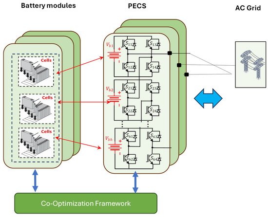
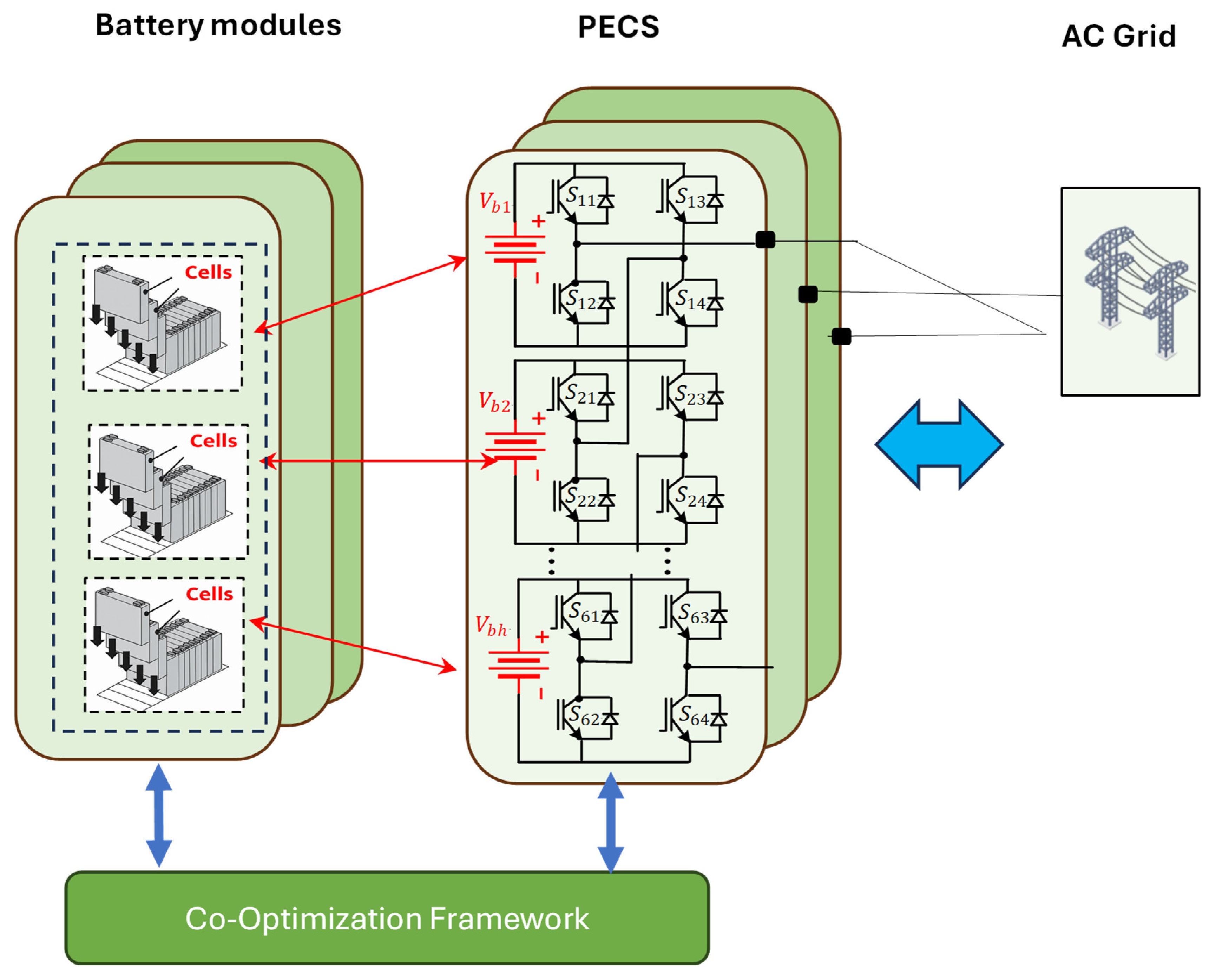
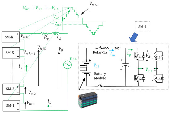
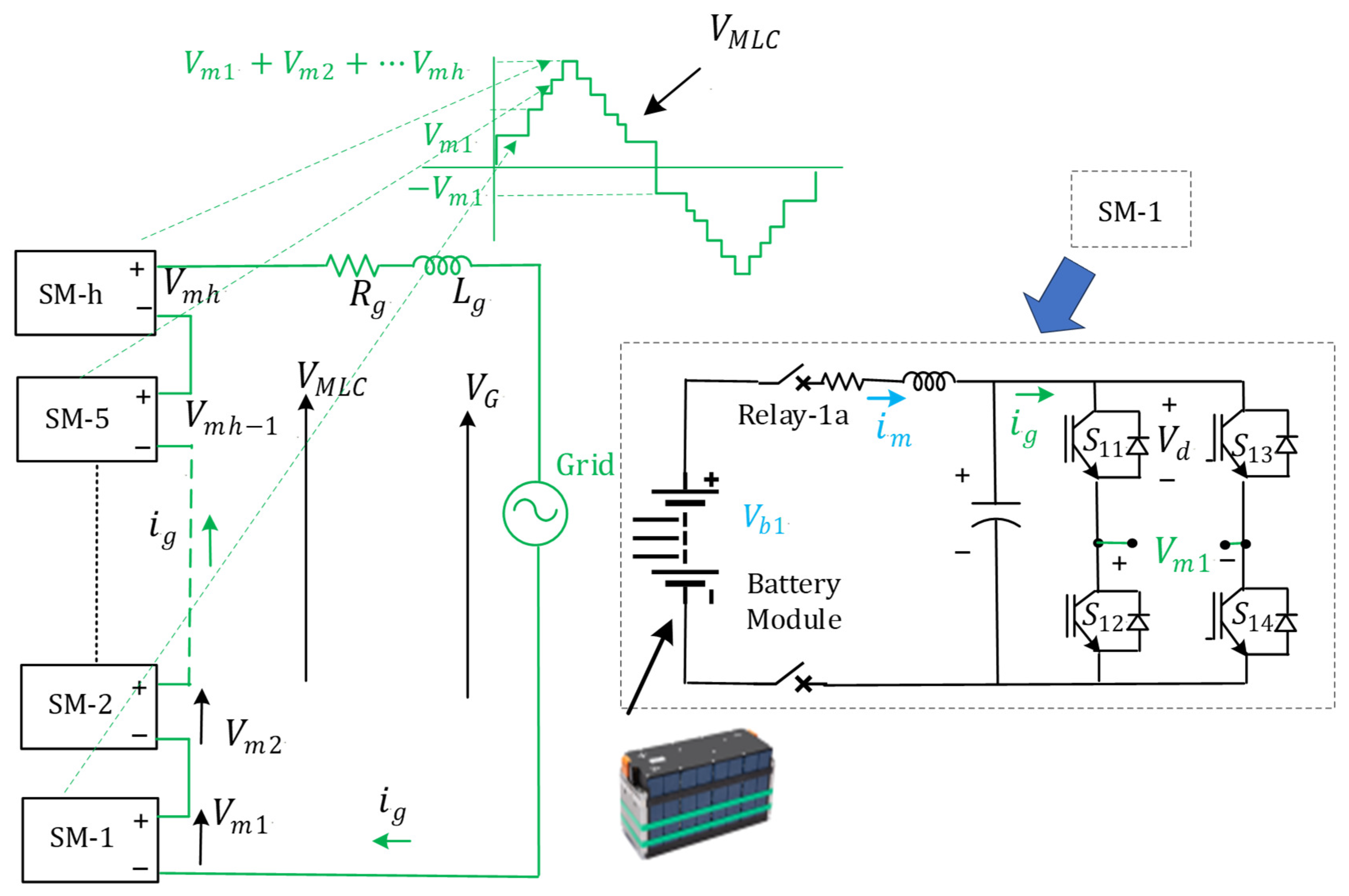
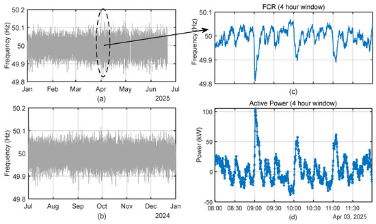
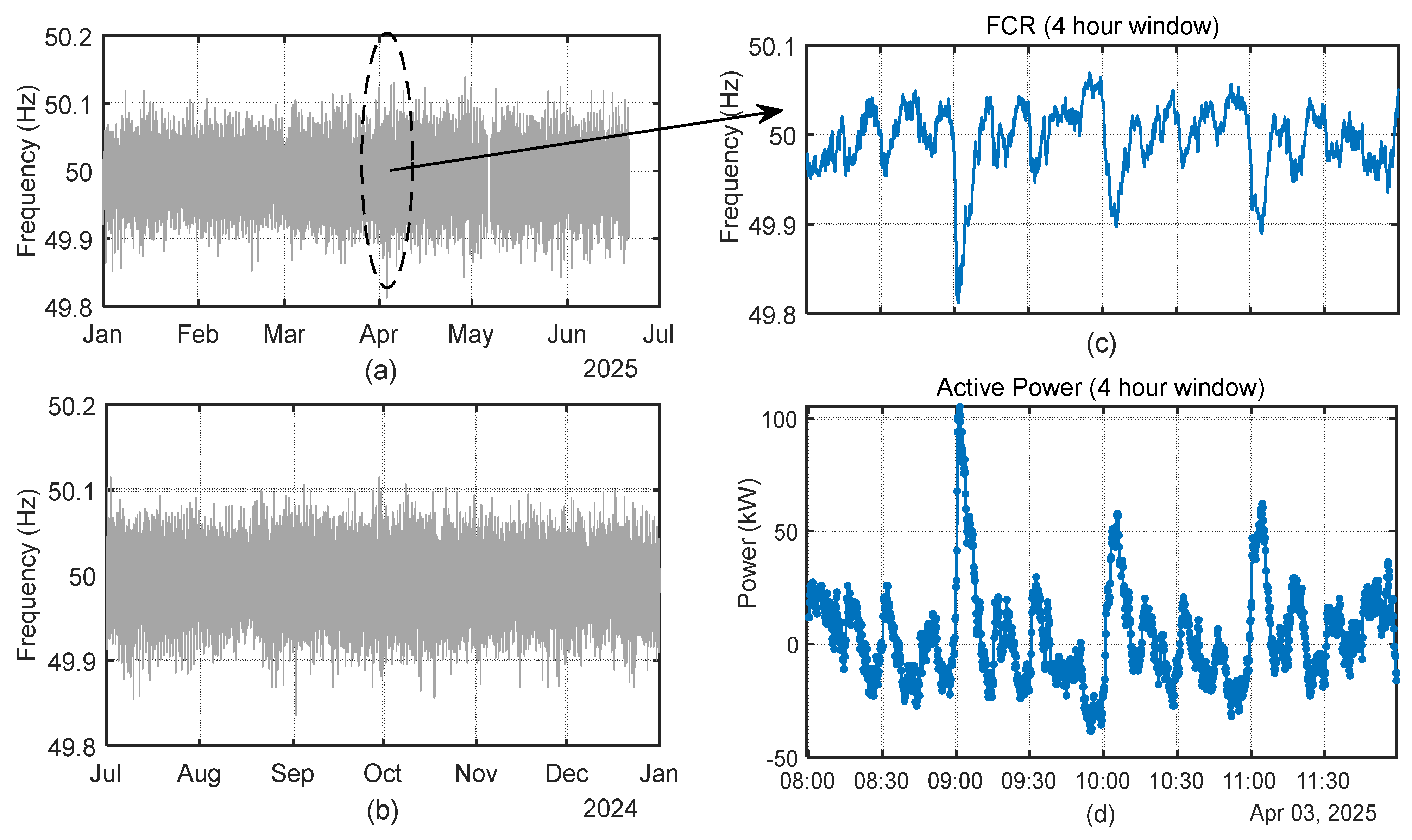
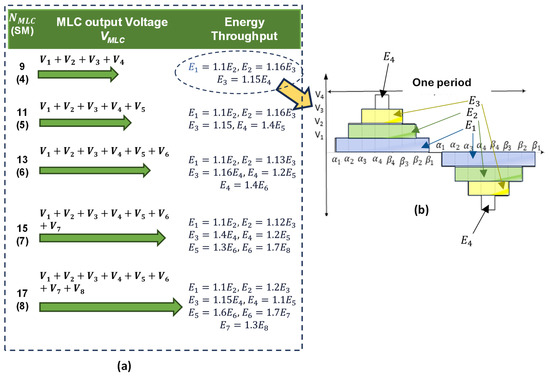
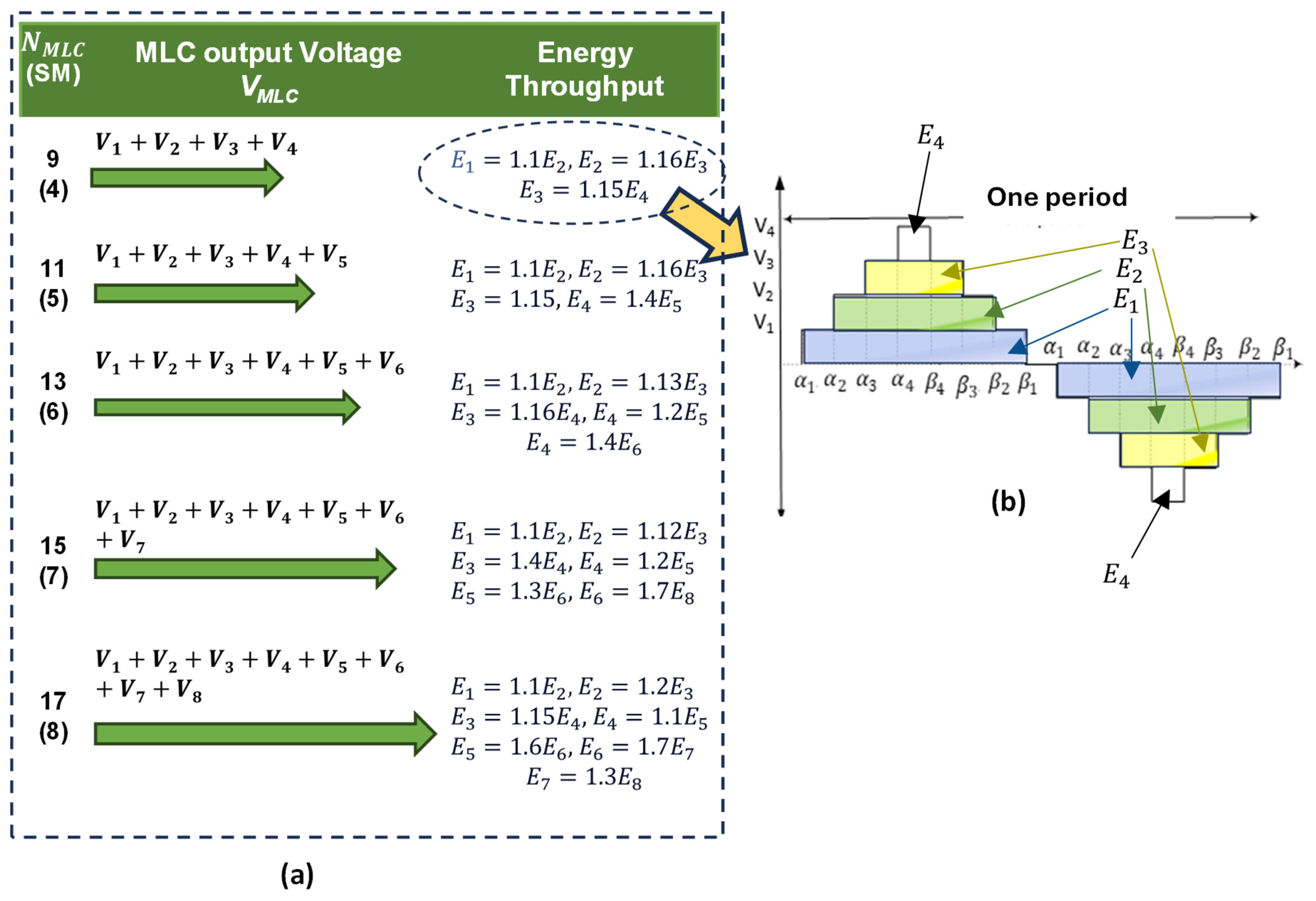
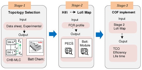
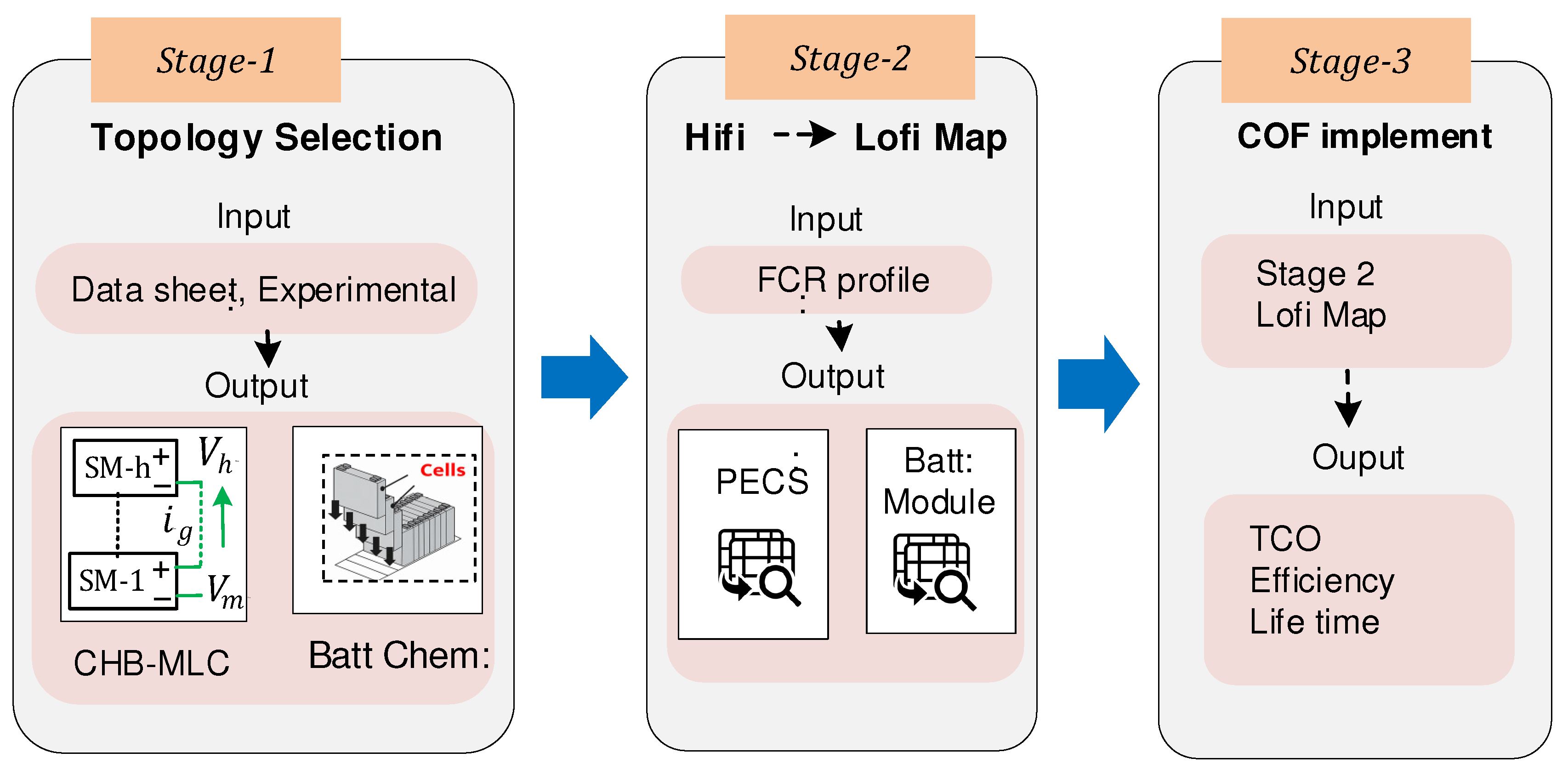
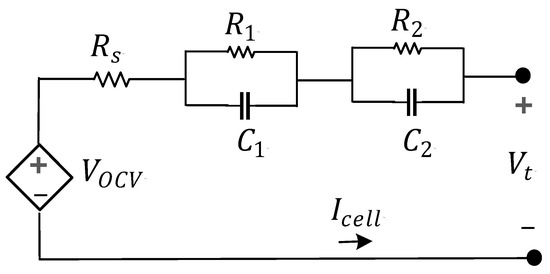
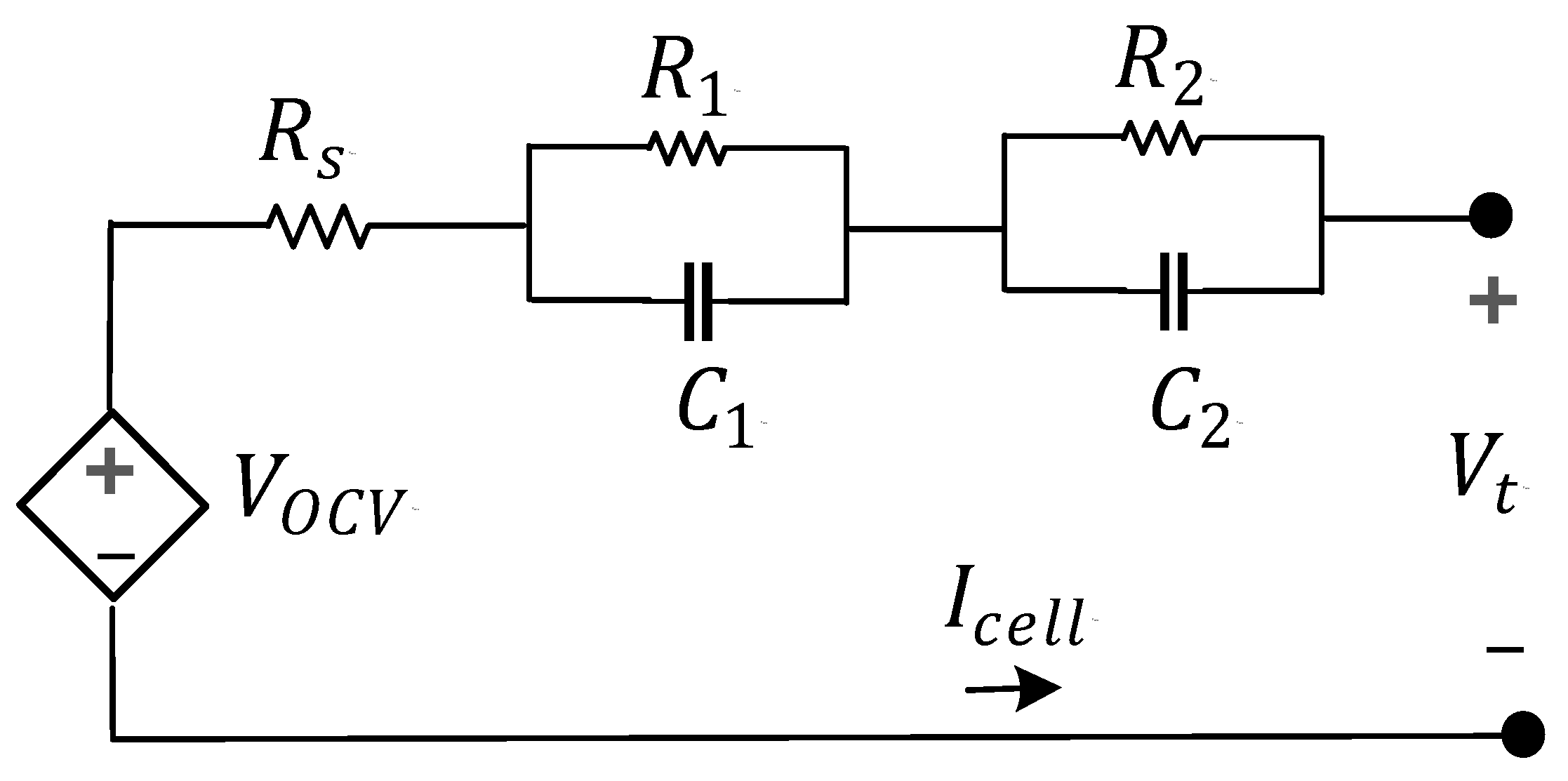
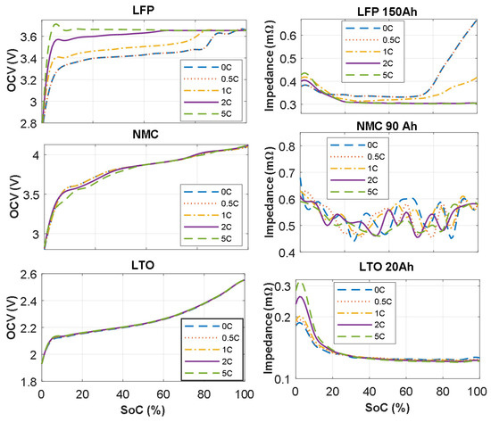
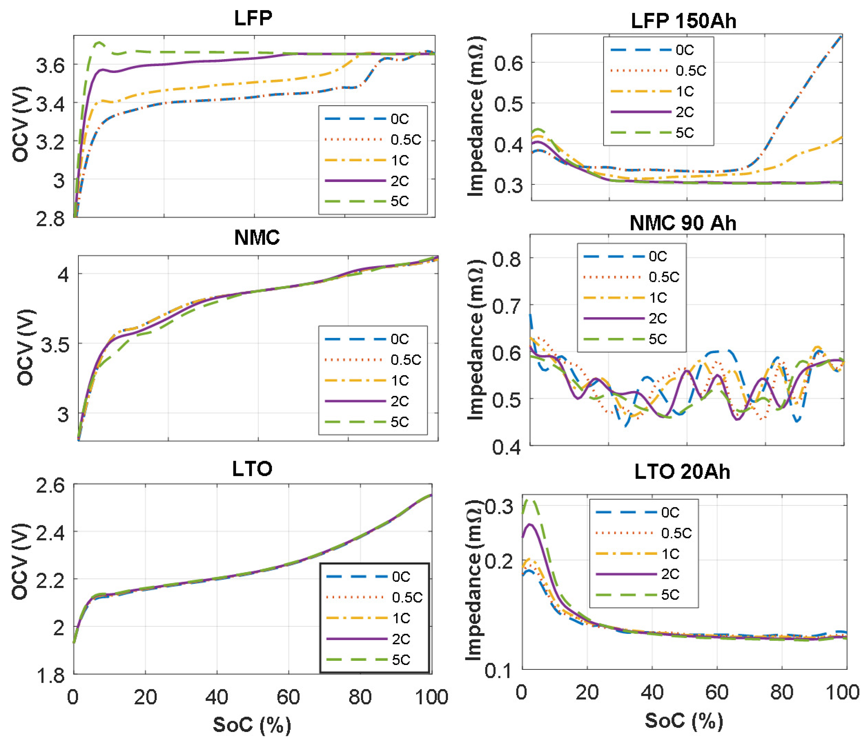
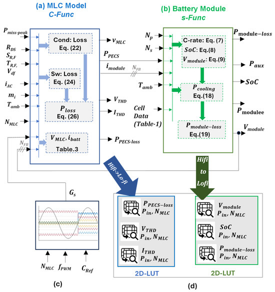
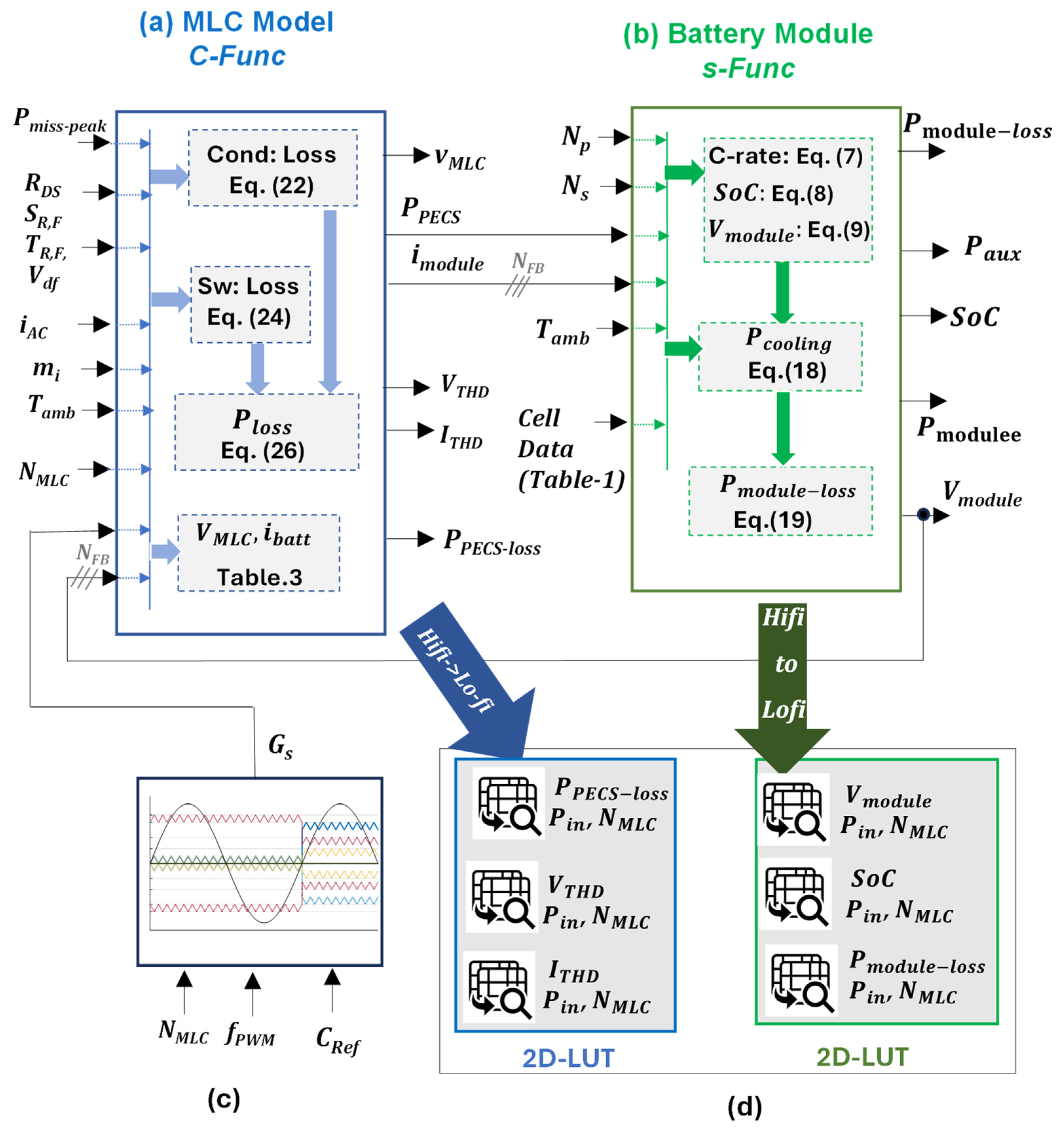
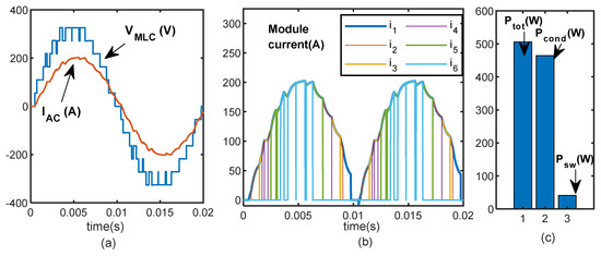
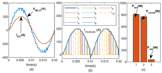
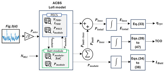
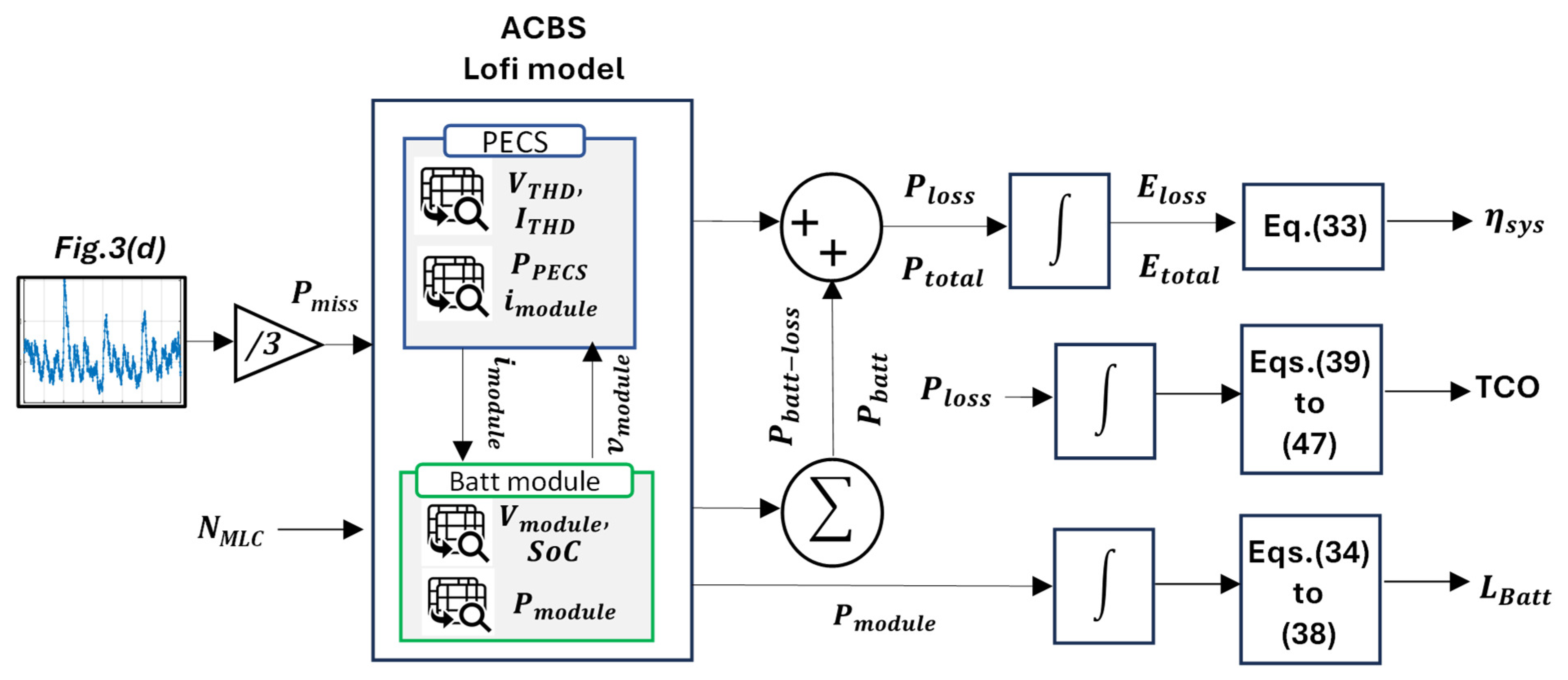
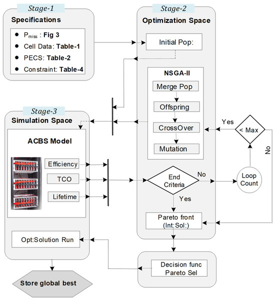
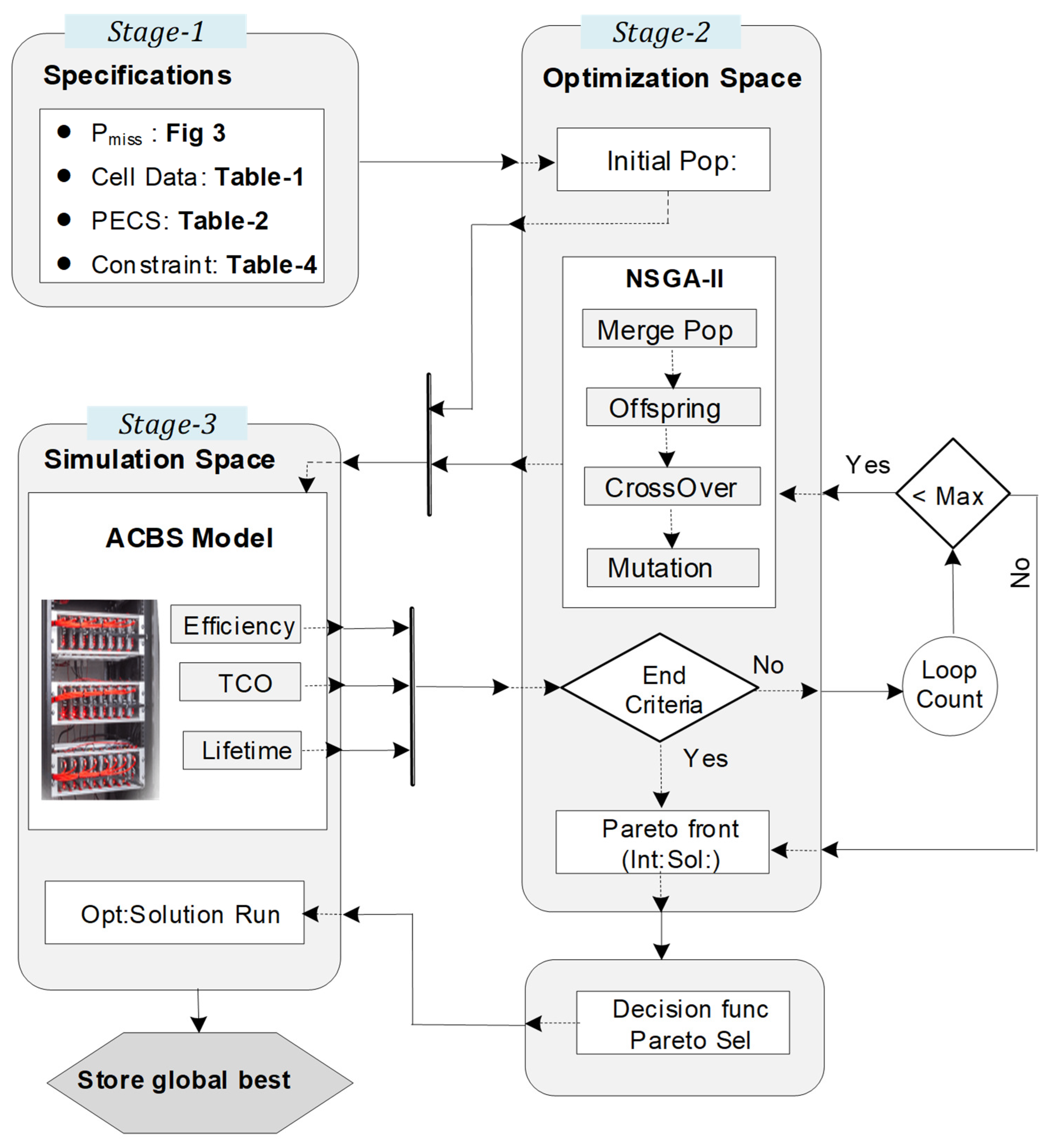
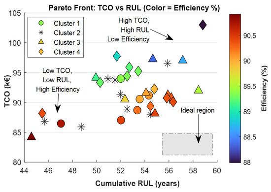
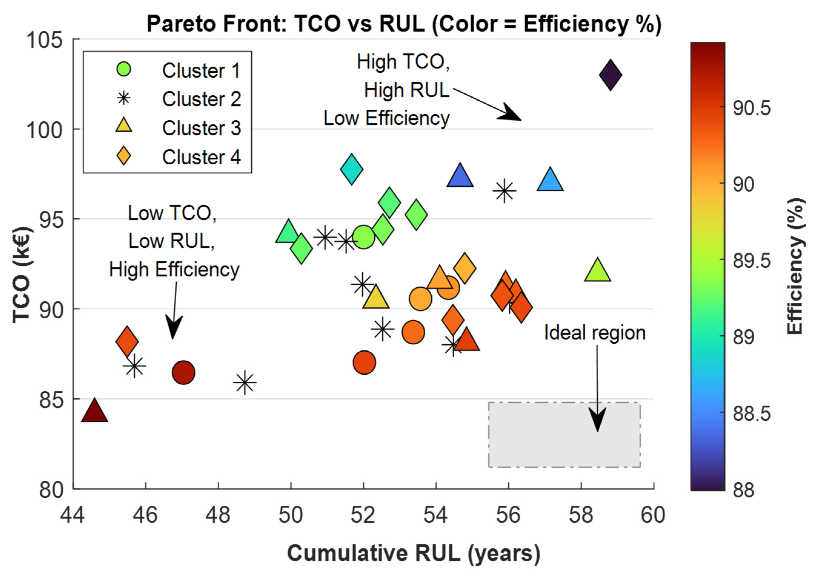
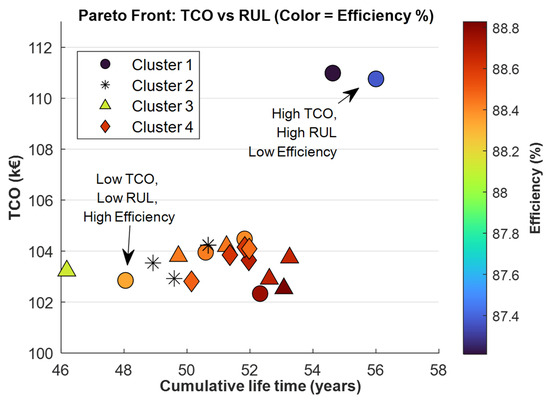
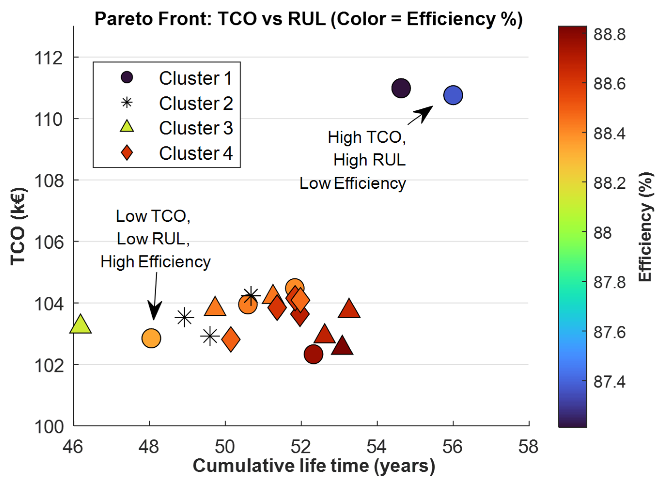
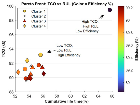
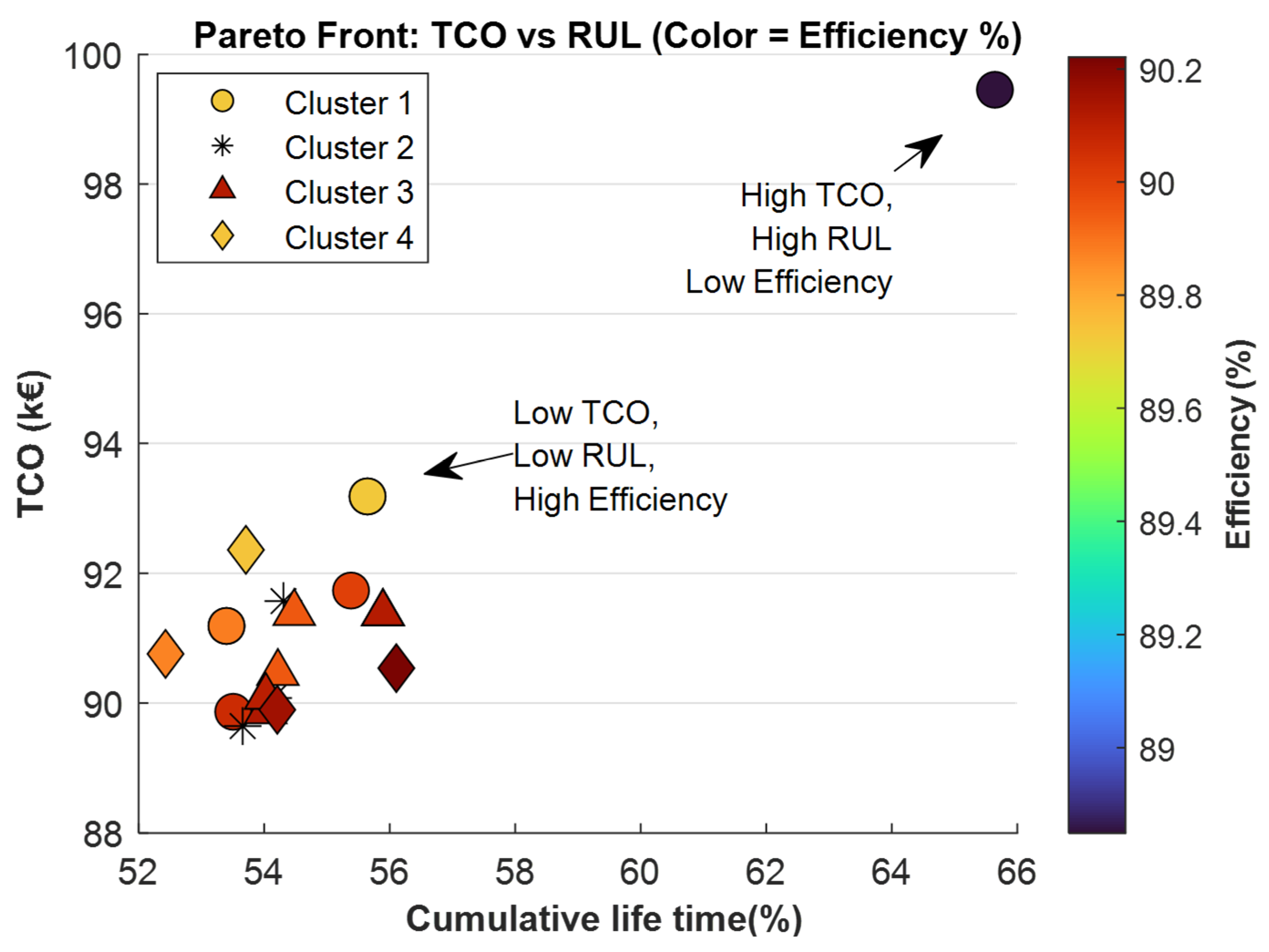
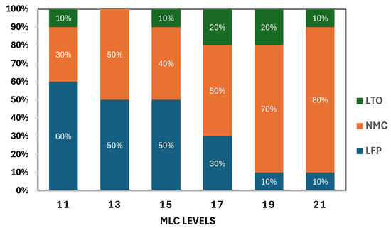
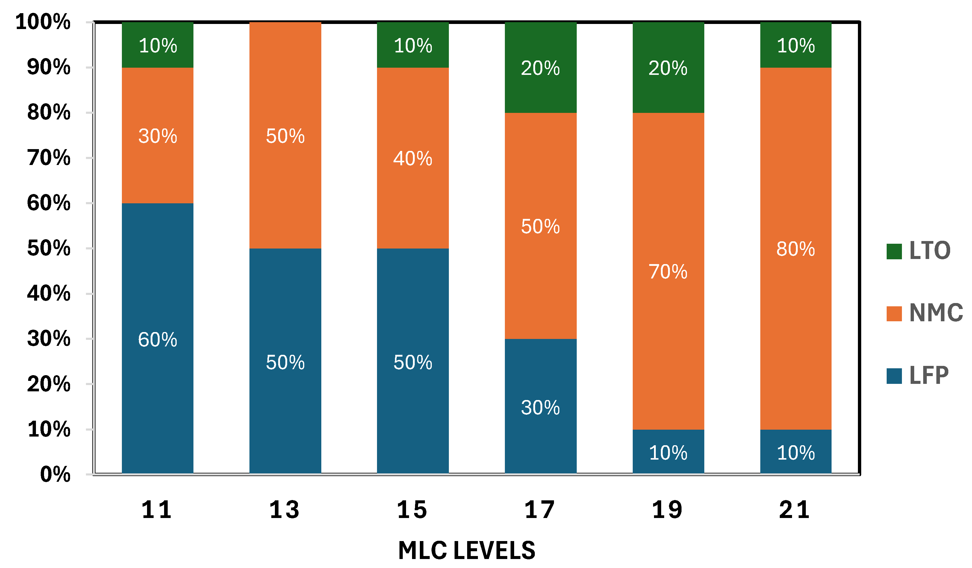
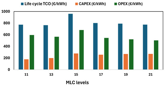
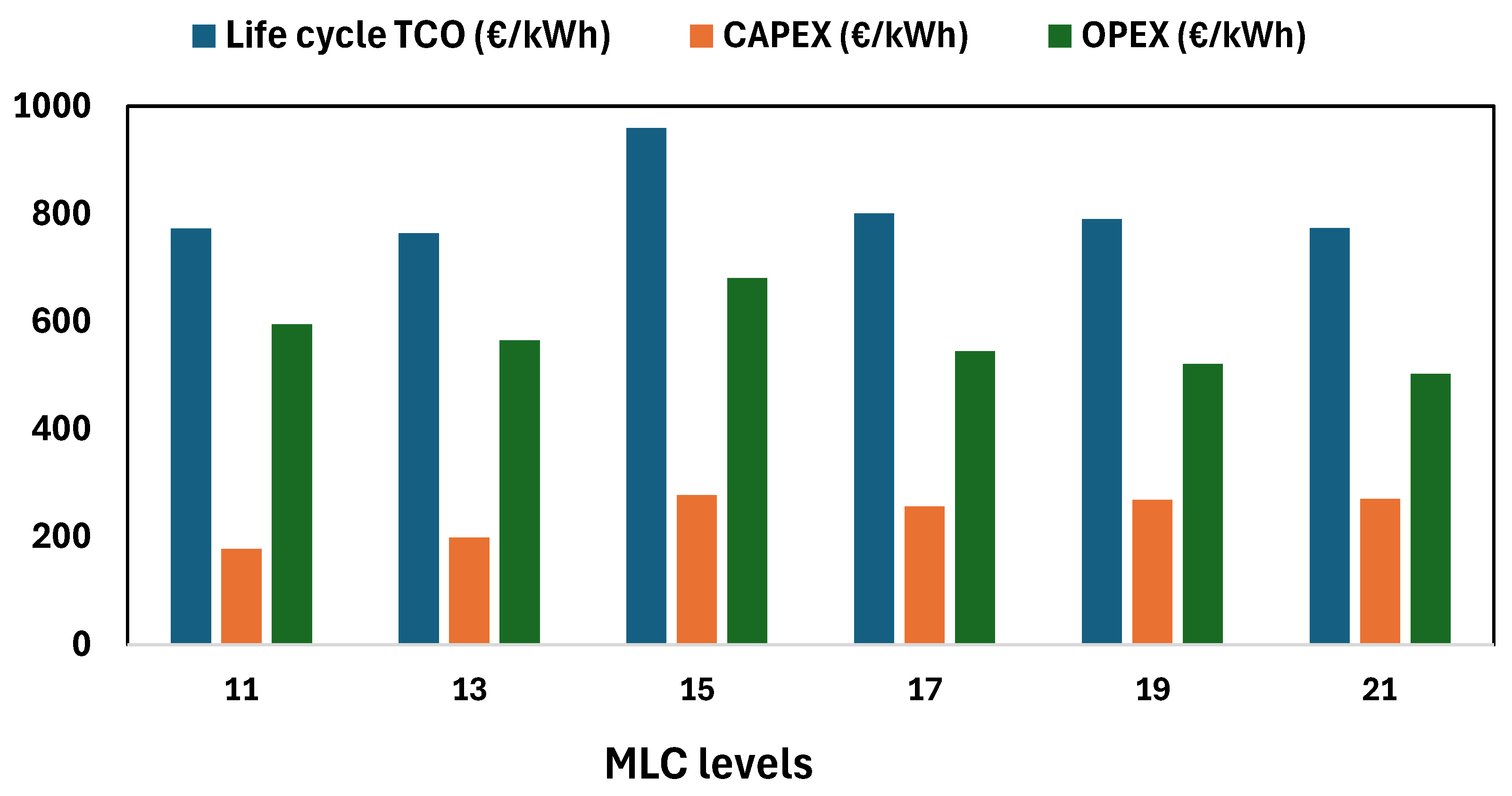
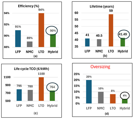
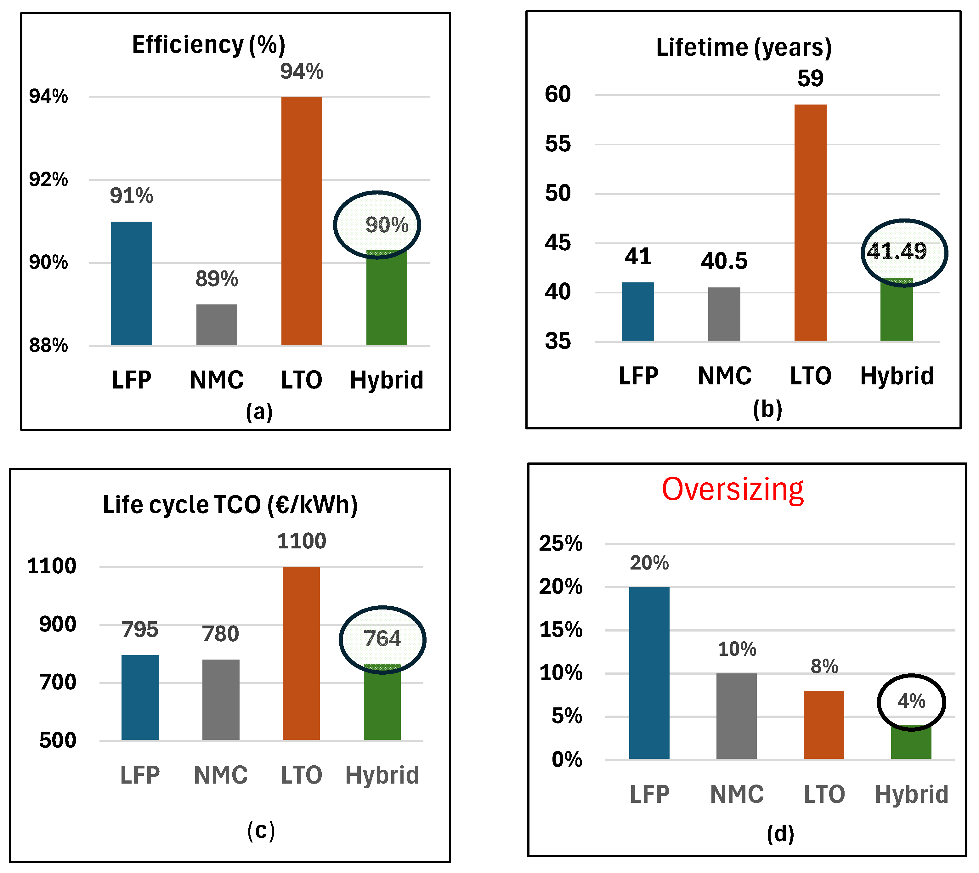
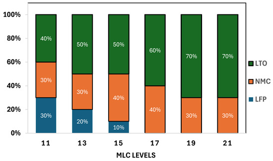
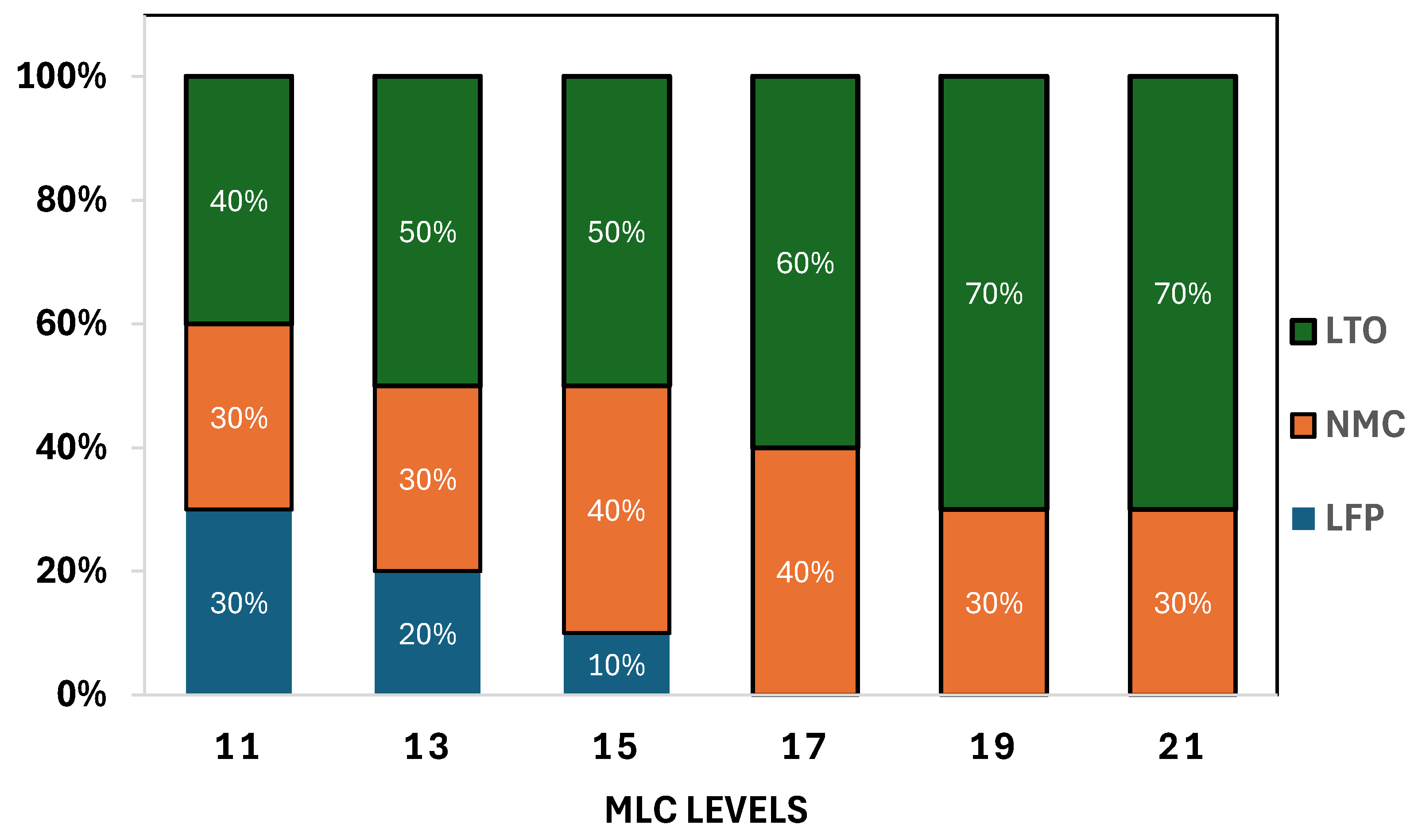
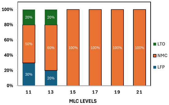
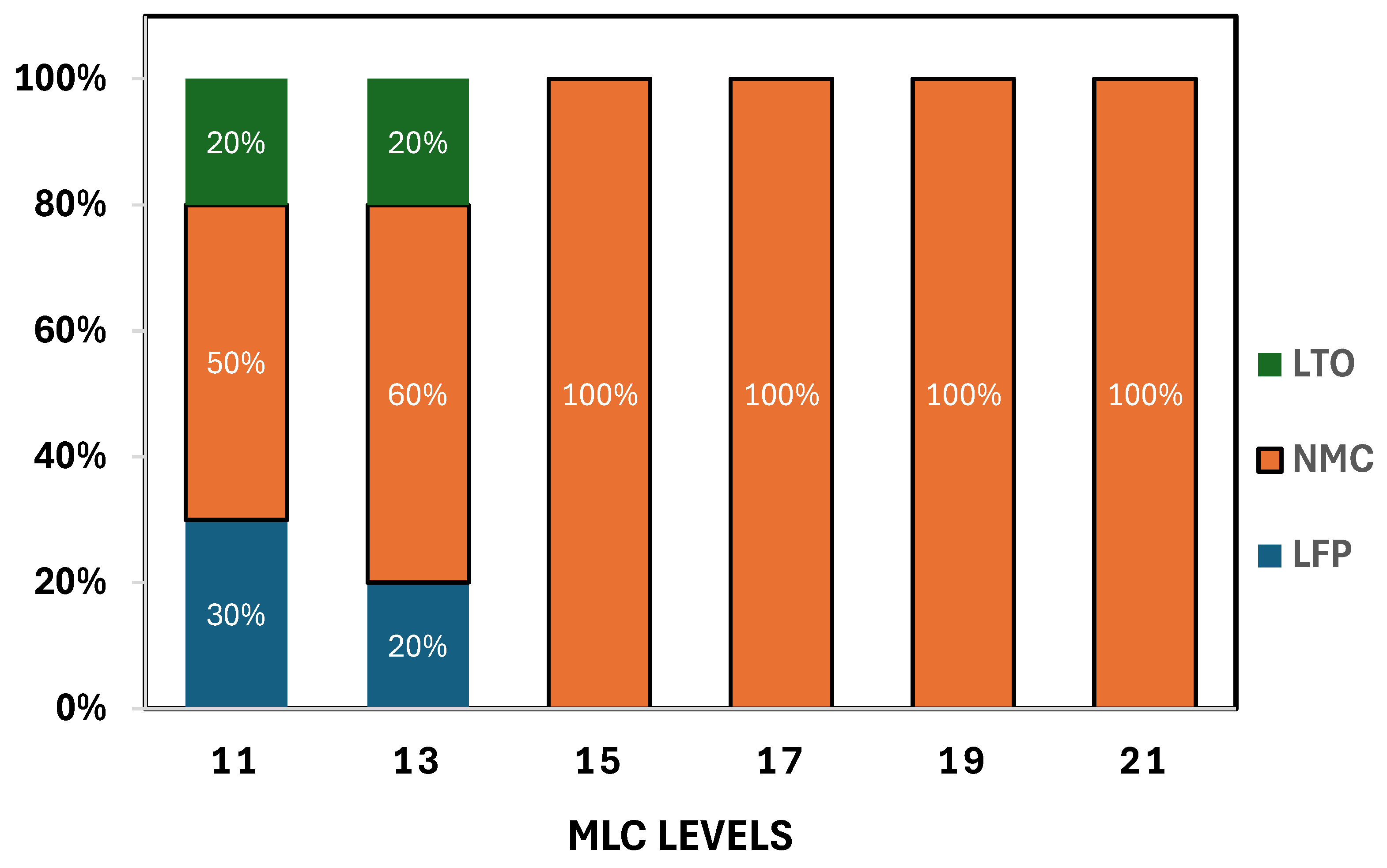

Disclaimer/Publisher’s Note: The statements, opinions and data contained in all publications are solely those of the individual author(s) and contributor(s) and not of MDPI and/or the editor(s). MDPI and/or the editor(s) disclaim responsibility for any injury to people or property resulting from any ideas, methods, instructions or products referred to in the content. |
© 2026 by the authors. Licensee MDPI, Basel, Switzerland. This article is an open access article distributed under the terms and conditions of the Creative Commons Attribution (CC BY) license.