


Abstract
Accurate photovoltaic (PV) power forecasting under extreme weather conditions remains challenging due to the non-stationary and multi-modal nature of meteorological influences. This study proposes a novel four-stage learning framework integrating signal decomposition, hyperparameter optimization, temporal dependency learning, and residual compensation to enhance forecasting resilience during El Niño–Southern Oscillation (ENSO) climate transitions. The framework employs CEEMDAN for fluctuation mode decoupling, TOC for global hyperparameter optimization, Transformer model for spatiotemporal dependency learning, and EEMD-GRU for error correction. Experimental validation utilized a comprehensive dataset from Australia’s Yulara power station comprising 104,269 samples at 5 min resolution throughout 2024, covering a complete ENSO transition period. Compared against baseline Transformer model and CNN-BiLSTM models, the proposed framework achieved nRMSE of 1.08%, 7.04%, and 2.81% under sunny, rainy, and sandstorm conditions, respectively, with corresponding R2 values of 0.99981, 0.99782, and 0.99947. Cross-year validation (2023 to 2025) demonstrated maintained performance with nRMSE ranging from 4.68% to 15.88% across different temporal splits. The framework’s modular architecture enables targeted handling of distinct physical processes governing different weather regimes, providing a structured approach for climate-resilient PV forecasting that maintains 2.56% energy consistency error while adapting to rapid meteorological shifts.
1. Introduction
The global energy transition is making the development and utilization of renewable energy a key pathway to addressing energy supply security and environmental protection concerns [1]. Among these, solar photovoltaic (PV) power generation technology has developed rapidly due to its abundant resources and continuously declining costs [2]. The International Energy Agency predicts that it will become the largest source of renewable energy by 2030 [3]. However, PV power generation is highly dependent on meteorological conditions and is sensitive to various factors such as solar irradiance, ambient temperature, cloud cover, and humidity. This inherent intermittency and variability pose severe challenges to the rational dispatch and stable operation of power grids [4,5].
Currently, the global climate system is undergoing significant anomalous changes. The year 2024 marks a transition from a strong El Niño event to a La Niña phenomenon, which is particularly influential in Australia. El Niño typically brings prolonged drought and increased solar radiation to Australia, whereas La Niña often leads to above-average rainfall and cloud cover [6,7]. Therefore, this study utilizes data from the Yulara power station in Australia to investigate the impacts of these transitions on PV power generation. Under such altered observational climate conditions, maintaining high accuracy and reliability in PV power forecasting models faces unprecedented challenges [8].
To address this challenge, PV power forecasting techniques have evolved into main approaches including physical models, statistical models, and deep learning models. Physical models, based on radiative transfer equations and cloud image analysis, offer high accuracy and clear physical interpretability under clear-sky conditions; however, their performance heavily relies on accurate meteorological inputs and their precision is limited under complex weather conditions [9]. Statistical and machine learning methods, such as Support Vector Machines, Random Forests, and Backpropagation Neural Networks, adopt a data-driven strategy that avoids complex physical modeling, but they typically require cumbersome feature engineering and exhibit limitations in nonlinear fitting capabilities [10,11,12]. In recent years, deep learning models, such as Long Short-Term Memory (LSTM) networks and Gated Recurrent Units (GRUs), have demonstrated significant advantages by leveraging automatic feature extraction and powerful temporal modeling capabilities [13,14,15]. Nevertheless, these conventional single models often struggle to uniformly capture the complex, nonlinear, and comprehensive dynamic characteristics between various atmospheric parameters and PV output, and they exhibit insufficient capability in handling multi-dimensional features [16,17]. To overcome the limitations of single models, hybrid models have significantly improved forecasting accuracy by integrating techniques such as signal decomposition, feature optimization, and deep learning. Signal decomposition algorithms are widely employed to handle the non-stationary characteristics of PV power, effectively reducing forecasting difficulty [18,19,20].
Although existing hybrid models have shown advances in fitting accuracy, most studies still mainly focus on optimizing model architecture to enhance data fitting precision. There is a general lack of in-depth research on how meteorological physical mechanisms systematically affect model performance under different weather conditions, especially in the context of variable weather patterns driven by large-scale climate modes like ENSO [21]. Studies have documented that accurately modeling PV output under distinct extreme weather conditions remains a significant challenge for conventional methods [22,23,24]. The absence of modeling approaches that are inherently resilient to these shifts leads to unstable performance during climate transition periods, severely compromising reliability and robustness in practical engineering applications [25]. Furthermore, the majority of existing research concentrates on point forecasts, while overlooking the crucial aspect of forecast error correction [26]. To provide a systematic comparison with existing approaches, Table 1 summarizes the key limitations of previous studies.
Table 1.
Current status of prediction methods.
Consequently, this study addresses a critical research gap by investigating the following research question: How can a modular forecasting framework maintain accuracy across rapidly shifting meteorological regimes during ENSO transitions, and what architectural principles enable such climate resilience?
We hypothesize that deconstructing the forecasting pipeline into four specialized stages—fluctuation mode decoupling, mapping relationship optimization, spatiotemporal dependency learning, and residual error compensation—will systematically address the distinct physical challenges posed by different weather scenarios. These stages operate in a sequential yet functionally complementary manner: the output from each stage serves as input to the next, creating an integrated processing chain. Specifically, the decomposition stage first separates the power signal into physically meaningful components; the optimization stage then identifies globally robust hyperparameters; the spatiotemporal learning stage processes the enhanced features; and finally, the error correction stage refines the predictions. This modular design is expected to achieve more accurate and resilient predictions compared to conventional unified models, as each stage can be optimized for specific aspects of the forecasting problem while maintaining synergistic integration within the overall framework. This study supports that a combination of a structured understanding of weather-dependent fluctuation modes and a modular framework design offers an effective path for constructing high-performance and climate-adaptive forecasting models. The unique contribution of this framework lies in providing a systematic methodology that addresses distinct physical challenges under complex meteorological conditions through four specialized stages, which differs from methods focused on purely model optimization.
To validate this hypothesis, we develop a novel four-stage forecasting framework and evaluate its performance under three distinct weather regimes (sunny, rainy, and sandstorm) during a complete ENSO transition year, comparing against established baseline models through comprehensive ablation studies. The Yulara photovoltaic power station was selected as the case study for this research due to its representative characteristics across multiple dimensions. Geographically, it is located in Australia’s arid zone (Köppen climate classification BWh), which experiences the pronounced ENSO impacts described above and represents a significant portion of Australia’s solar development potential. With a capacity of 1.8 MW, the plant represents a typical utility-scale solar installation in the Australian National Electricity Market. Its location in the Northern Territory provides critical insights into grid integration challenges in regions with high solar penetration but limited conventional generation backup. Furthermore, the site’s exposure to both dust storms and rainfall variability during ENSO transitions makes it an ideal natural laboratory for testing climate-resilient forecasting approaches under realistic extreme weather conditions.
It should be noted that this study focuses on short-term forecasting with a prediction horizon of 24 h, utilizing the 5 min temporal resolution of the dataset to generate 288 consecutive forecast points. This short-term forecasting framework is particularly relevant for addressing the rapid meteorological shifts characteristic of ENSO transitions, where cloud cover changes and dust storm events can significantly impact power generation within hours. The selected forecasting horizon aligns with the operational needs of grid operators for day-ahead scheduling and real-time balancing, while the evaluation metrics (nRMSE, MAE, and R2) are appropriately suited for assessing short-term forecasting performance at this temporal scale.
2. Data Analysis and Weather Scenario Characteristics
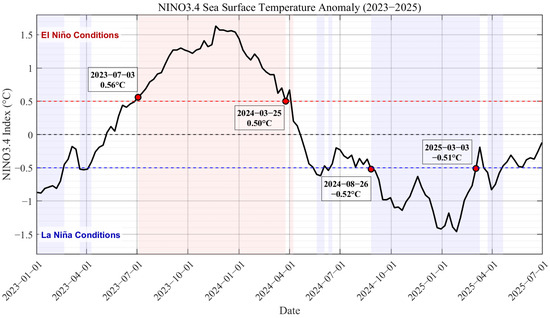
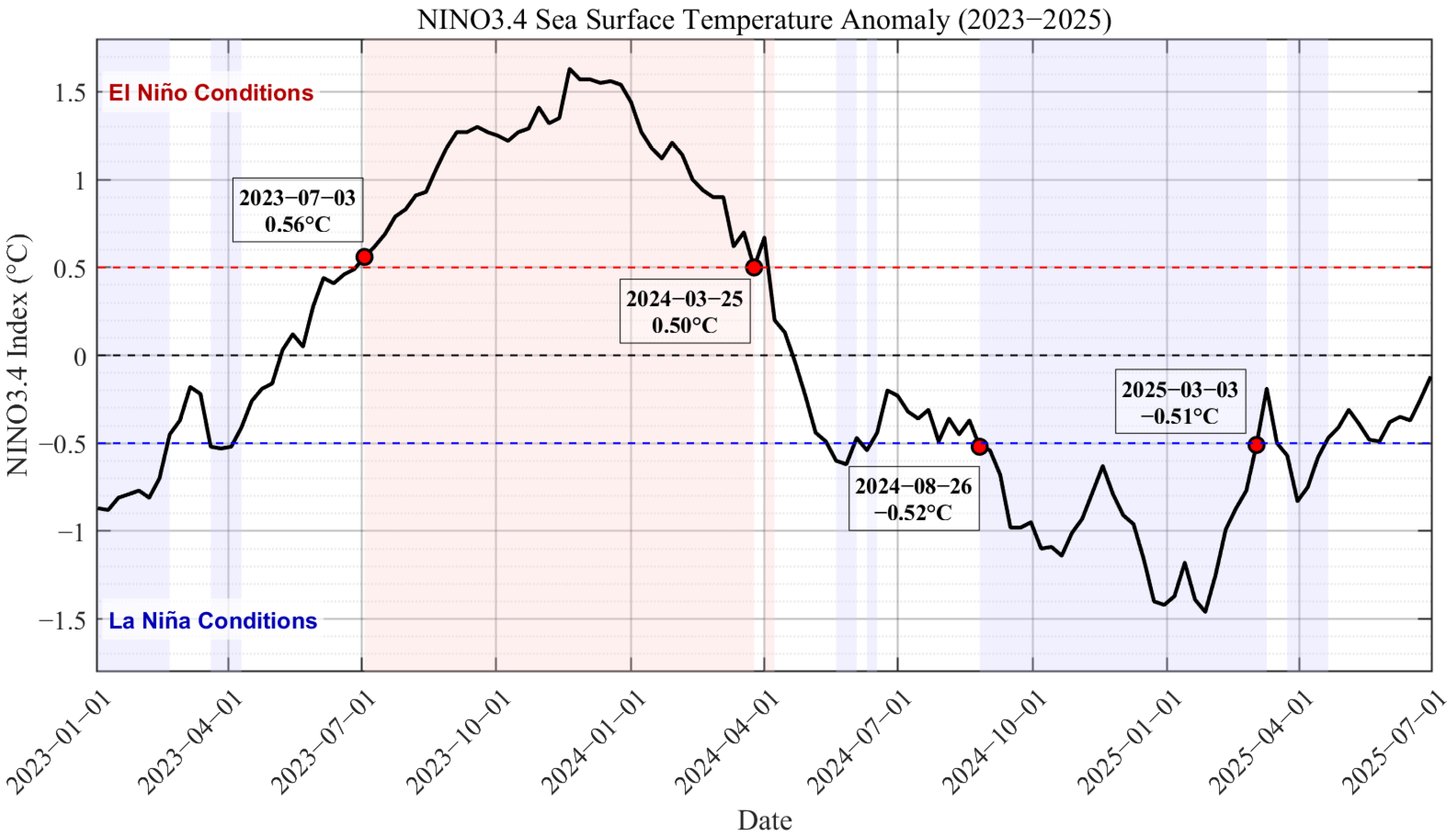
The data used in this study originates from the measured dataset of the Yulara photovoltaic power station in Australia for 2024, with a temporal resolution of 5 min, comprising 104,269 samples in total [27]. To quantitatively characterize the climatic background of the dataset and justify the study period, we refer to the weekly NINO3.4 index provided by the Australian Bureau of Meteorology from 2023 to 2025, based on the established threshold of ±0.5 °C for at least five consecutive overlapping three-month periods to define ENSO events [28]. As shown in Figure 1, the NINO3.4 Sea Surface Temperature (SST) anomaly illustrates the complete evolution of a phase transition. According to the threshold standard defined by the Australian Bureau of Meteorology (anomalies sustained above +0.5 °C or below −0.5 °C), an El Niño event was established in July 2023 (0.56 °C) and persisted through the first quarter of 2024. A rapid decay occurred subsequently, dropping below the +0.5 °C threshold by late March 2024. Following a brief neutral phase, the index fell below −0.5 °C in August 2024 (−0.52 °C), marking the onset of La Niña conditions.
Figure 1.
NINO3.4 sea surface temperature anomaly (2023–2025). The red background is the dominant time of El Niño, and the blue background is the dominant time of La Niña. The red dotted line and the blue dotted line are the thresholds for El Niño and La Niña conditions, respectively.
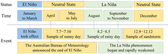
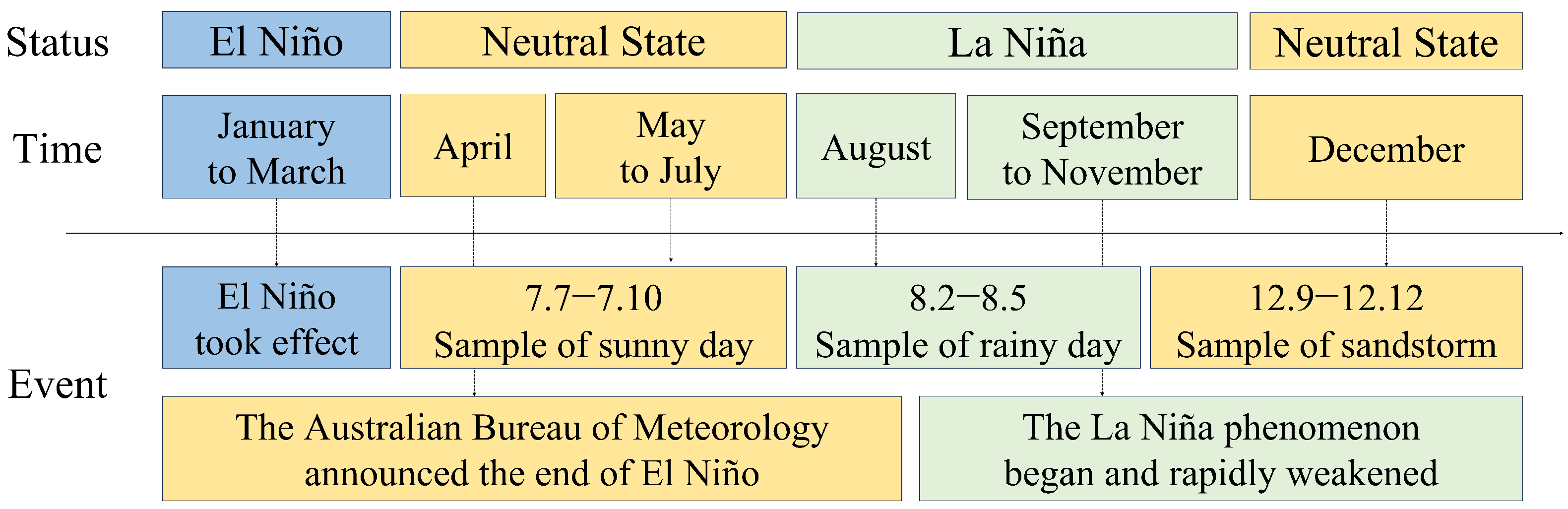
As shown in Figure 2, this dataset comprehensively records a typical climatic year marked by the transition from strong El Niño to La Niña. It encompasses seven meteorological variables: global horizontal irradiance, ambient temperature, wind speed, wind direction, maximum wind speed, rainfall, and atmospheric pressure, along with the target variable of PV power. This unique temporal coverage enables the dataset to capture two distinct physical backgrounds induced by the ENSO phase transition, including the clear, dry, high-radiation conditions dominated by El Niño and the cloudy, rainy, high-humidity conditions associated with La Niña. The stark contrast between these scenarios causes the power data to exhibit non-stationarity and high variability, presenting substantial challenges for forecasting models and underscoring the need for a resilient framework [29].
Figure 2.
Climate events and sample points in Australia in 2024.
During the data preprocessing stage, rigorous quality control and cleaning were performed on the raw data, including the removal of duplicate records and the correction of outliers that exceeded the theoretical maximum power. To ensure the rigor of time series forecasting and prevent any data leakage from the future, the dataset was split chronologically. The first 50% of the samples, corresponding to data from January to June 2024, constituted the training set, while the latter 50%, corresponding to data from July to December 2024, formed the test set. To eliminate the influence of different feature scales on model training, the min–max normalization method was applied. Using the statistics (minimum and maximum values) computed solely from the training set, all features in both the training and test sets were mapped to the [0, 1] interval. This procedure ensures that the normalization of the test set does not incorporate any information from its own distribution, adhering to standard practices in time series forecasting. The normalized equation is as follows:
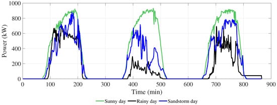
To visually demonstrate the physical challenges inherent in the forecasting task, Figure 3 displays the power curves extracted under three typical weather conditions, clear sky, precipitation, and dust storm, with their corresponding sample dates annotated in Figure 2.
Figure 3.
PV power curve under three typical weather conditions.
Power fluctuation patterns vary systematically with weather regimes, reflecting distinct underlying physical processes. Clear-sky conditions produce smooth curves governed by astronomical cycles, while rainy conditions exhibit rapid fluctuations due to cloud–radiation interactions [30,31]. Dust storms show complex oscillations indicative of multi-factor coupling [32].
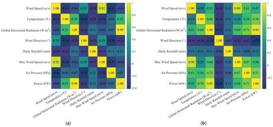
To quantitatively elucidate the dominant factors influencing PV output under different weather conditions, this study calculated the Pearson correlation coefficients between various meteorological variables and the power output, and plotted the corresponding correlation matrix shown in Figure 4.
Figure 4.
Pearson correlation coefficients between variables in rainy day (a) and sandstorm day (b).
In Figure 4a, under rainy conditions, the correlation coefficient between PV power and Global Horizontal Irradiance (GHI) is as high as 0.99. This indicates that in such weather, the influence of clouds on radiation is the dominant physical process governing power fluctuations. The core forecasting challenge lies in accurately isolating the power fluctuations determined by the physical process of cloud cluster movement from the radiation signal perturbed by clouds. The situation becomes considerably more complex under dust storm conditions, as shown in Figure 4b. Although the correlation between power and radiation remains the highest, it is lower than under precipitation conditions. Currently, the correlations between power and both temperature and air pressure have increased markedly, reaching 0.7. This suggests that the power output during dust storms constitutes a typical multi-physics factor coupled system. Dust particle accumulation on the panel surface affects transmittance, temperature influences PV module efficiency, and atmospheric pressure fluctuations reflect changes in the weather systems accompanying dust storms. These factors collectively create a nonlinear and difficult-to-decouple forecasting environment.
The aforementioned analysis, grounded in the established physical principles of cloud modulation of solar radiation and the multi-factor coupling in dust storms, demonstrates that a PV power forecasting model must be capable of adapting to three distinct physical regimes [30,31]. These observed regimes are not merely data patterns but manifestations of specific, well-documented atmospheric processes. This understanding forms the direct rationale for our model design: each regime presents a unique forecasting challenge that necessitates a targeted computational strategy, as detailed in the following section.
3. Four-Stage Forecasting Framework
The analysis in Section 2 delineates three predominant weather regimes—clear-sky, rainy, and dust storm—each exhibiting distinct power fluctuation patterns. The core of our forecasting strategy is to treat these regimes not merely as data categories but as manifestations of different underlying physical processes. The clear-sky regime is governed by deterministic astronomical cycles, the rainy regime by the radiative modulation of moving cloud systems, and the dust storm regime by the nonlinear coupling of multiple atmospheric factors.
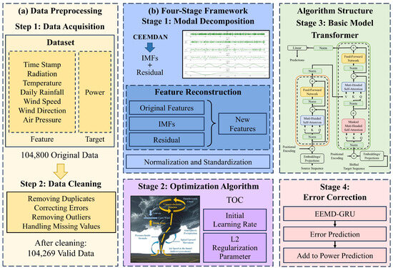
This analysis of distinct weather scenarios informs our modeling approach, which is designed to maintain forecasting accuracy despite rapid shifts in meteorological conditions. It reveals that a one-size-fits-all model is inadequate because the fundamental driver of power variability changes with the weather scenario. Therefore, we propose a four-stage forecasting framework that is structurally designed to learn and adapt to these regime-specific physical characteristics. The framework deconstructs the complex forecasting problem into four targeted stages, each addressing a key challenge identified through our climate-based analysis. The overall workflow of the framework is illustrated in Figure 5, operating through an integrated four-stage pipeline. The process begins with data acquisition and preprocessing, followed by sequential execution of the specialized modules. In the fluctuation mode decoupling stage, CEEMDAN decomposes the power signal into intrinsic mode functions and residual components. These are combined with meteorological variables to form an enriched feature set for subsequent modeling. This research hypothesizes that decomposing the forecasting process into four specialized stages—fluctuation mode decoupling, mapping optimization, spatiotemporal dependency learning, and residual error compensation—allows for a systematic approach to the unique physical challenges posed by different weather scenarios. For instance, the decoupling stage (CEEMDAN) was selected as a physical fluctuation mode decomposer to separate non-stationary features in the signal caused by distinct physical processes (e.g., diurnal cycle, cloud movement).
Figure 5.
Algorithm framework. All modules in the framework are executed sequentially. The arrows indicate the direction of data flow rather than conditional or optional computational paths. No bypass or skipping of stages occurs during model execution.
The mapping relationship optimization stage employs TOC to identify optimal hyperparameters, which configure the Transformer model in the spatiotemporal dependency learning stage. After main model training, the residual error compensation stage trains an EEMD-GRU model to correct systematic biases. During forecasting, new data undergoes identical decomposition before sequential processing through both main and error correction models, with their outputs combined to produce the final prediction.
This coordinated architecture enables each module to address specific forecasting challenges while maintaining unified data flow, collectively enhancing prediction accuracy across diverse meteorological conditions.
3.1. Fluctuation Mode Decoupling
This stage aims to address the difficulties caused by the non-stationary nature of the original power sequence for model feature extraction. The integration of diverse meteorological influences—such as diurnal cycles, cloud movements, and dust disturbances—within a single signal complicates the direct learning of consistent patterns under variable weather conditions.
The framework employs Complete Ensemble Empirical Mode Decomposition with Adaptive Noise (CEEMDAN) as a physical fluctuation mode decoupler. CEEMDAN was selected over other decomposition techniques for two primary reasons: first, it effectively mitigates the problem of mode mixing that is prevalent in EMD; second, it reduces the reconstruction error and computational cost compared to EEMD by adaptively adding white noise at each decomposition stage [18]. These properties make it particularly suitable for generating a stable and complete set of sub-signals from the highly non-stationary PV power data. CEEMDAN can adaptively decompose the complex original power signal into a series of Intrinsic Mode Functions (IMFs) and a residual component [33]. The decomposition process can be mathematically represented as:
where is the original power signal, is the k-th intrinsic mode function, K is the total number of IMFs, and is the final residual.
This stage is not merely a mathematical transformation but serves to dissect the composite signal into simpler components. High-frequency IMFs often capture transient disturbances (e.g., passing clouds), mid-frequency IMFs may reflect mesoscale weather evolution, while low-frequency IMFs and the residual primarily represent deterministic trends (e.g., diurnal cycles). Through this decoupling, downstream models receive sub-signals with narrower frequency bands and trends. This separation can alleviate the challenge of modeling the original non-stationary signal directly, potentially facilitating a more effective learning process for the subsequent model [33,34].
3.2. Mapping Relationship Optimization
The correlation analysis in Section 2 indicates that the mapping relationship between input features and power output is dynamic and varies across different physical weather regimes. Models with fixed parameters struggle to maintain optimal performance across all scenarios.
Consequently, this framework introduces a global optimizer whose core task is to search for model hyperparameters suitable for all-weather scenarios. This paper employs the Tornado Optimizer with Coriolis force (TOC) as a representative global optimizer. It is critical to note that this optimization module is general. The TOC algorithm is used here as an exemplar, and the framework is designed to be fully compatible with any other hyperparameter optimization technique (e.g., Bayesian Optimization, Grid Search), allowing users to substitute their preferred method based on computational needs or domain familiarity. This optimizer operates on the complete training set encompassing all weather types, using the overall prediction’s Mean Squared Error (MSE) as the optimization objective to find the global optimum for key hyperparameters such as the initial learning rate and L2 regularization parameter [35]. The goal of this parameter set is to achieve an optimal balance across diverse climatic regimes, such as radiation-dominated and multi-factor coupled environments, thereby enhancing the model’s resilience to weather variability and preventing overfitting to any single meteorological pattern.
3.3. Spatiotemporal Dependency Learning
This stage employs a Transformer model as the core spatiotemporal physical dependency learner, responsible for uniformly learning the complex spatiotemporal dependencies between the decoupled power components and multi-dimensional meteorological features across different physical modes.
The self-attention mechanism of this learner effectively captures global dependencies within long sequences, overcoming the limitations of traditional recurrent neural networks in modeling long-range dependencies. Its multi-head attention structure enables it to simultaneously attend to interactions among multiple physical variables, such as irradiance, temperature, and air pressure, across different time scales [36]. Consequently, this learner can simultaneously acquire knowledge of the deterministic physical trends characteristic of clear-sky radiative days, the rapid disturbance and recovery dynamics of precipitating cloud systems, and the multi-factor coupled oscillation patterns observed during dust storm conditions from the decomposed data.
3.4. Residual Error Compensation
This stage is crucial for the framework to achieve high accuracy and robustness. Its physical essence lies in compensating for the complex physical effects that the main model fails to fully capture due to its limited learning capacity, particularly under multi-field coupled weather conditions.
The additive error model is adopted as a principled and parsimonious approach commonly used in forecast error correction [37]. This model posits that the final prediction can be decomposed into the main model’s output and a learnable bias term. Its widespread use is justified by its effectiveness in numerous applications, where the residual sequence is treated as a target for secondary modeling.
In this framework, the error sequence of the main model is treated as a representation of the under-learned physical phenomena. A secondary learning model, which is relatively more efficient as it operates on the simpler residual sequence rather than the full feature set, is introduced to perform a focused prediction, yielding an error correction term . This paper employs EEMD-GRU as an example for this purpose [38]. The final prediction is given by this equation:
where is the initial prediction from the main model, and is the predicted residual error from the error correction module.
Instead of repredicting the power, this module focuses on capturing and correcting the residual, physically-patterned deviations from the main model. It adds a compensation mechanism for the model’s learning insufficiencies to the entire framework, thereby pushing the prediction accuracy to its limit.
4. Experiments and Analysis
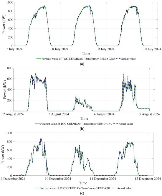
To comprehensively evaluate the physical modeling capability of the proposed framework, experiments were conducted on the test set covering the complete ENSO transition year. Three typical weather episodes, sunny day, rainy day, and sandstorm, were selected for validation. These correspond to power fluctuations with three distinct physical natures, deterministic physical processes, radiation-dominated environments, and multi-factor nonlinear coupled systems, respectively, as outlined in Table 2. The forecasting results of the proposed framework under these three weather conditions are shown in Figure 6, visually demonstrating the model’s ability to uniformly adapt to different physical fluctuation patterns and exhibit excellent tracking performance across all scenarios.
Table 2.
Corresponding relationship between weather and meteorological physical process.
Figure 6.
Forecast results in sunny day (a), rainy day (b), and sandstorm day (c).
4.1. Comparative Experiments
To quantitatively evaluate the contribution of each stage in the framework towards enhancing physical modeling capability, we designed a progressive ablation study. Using the Transformer model as the baseline model, components were incrementally added. First, the CEEMDAN decomposition, then the TOC hyperparameter optimization, and finally the EEMD-GRU error correction module, forming four comparative models. All models were trained using the Adam optimizer with a batch size of 64 and a maximum of 50 epochs. An early stopping strategy was implemented to prevent overfitting. All models were trained on the same complete training set and evaluated on the same test set using Normalized Root Mean Square Error (nRMSE), Mean Absolute Error (MAE), and the Coefficient of Determination (), which are defined as follows:
where is the actual value, is the predicted value, is the mean of the actual values, and N is the number of samples.
The results, presented in Table 3, show that the complete framework achieved the optimal forecasting performance across all three physical scenarios.
Table 3.
Indicators of Transformer-based models under different conditions.
An objective discussion is necessary regarding the extremely high metrics achieved by the model under clear-sky conditions (e.g., nRMSE of 1.08%, R2 of 0.99981). Under clear-sky conditions, the PV power curve is primarily driven by deterministic astronomical cycles, and its variability is low, allowing the model to capture its main pattern with high precision. However, the model’s performance metrics are lower but remain robust under the variable conditions of rain (nRMSE 7.04%) and sandstorm (nRMSE 2.81%), suggesting that the model has not been overly dependent on a single, stable data distribution. Furthermore, the cross-year validation provides preliminary evidence suggesting the framework possesses certain temporal robustness, which helps mitigate concerns about excessive optimization on a specific dataset.
To demonstrate that the performance improvement of the framework stems primarily from its architecture rather than the choice of a specific learner, we replaced the Transformer model in the framework with a CNN-BiLSTM, forming the TOC-CEEMDAN-CNN-BiLSTM-EEMD-GRU model for comparison. The CNN-BiLSTM can utilize convolutional layers to extract local spatial features and capture temporal dependencies via a Bidirectional LSTM, representing another widely used spatiotemporal model [39,40,41].
As can be observed from Table 4, the complete framework based on CNN-BiLSTM also achieved high prediction performance comparable to the Transformer model version across all weather scenarios. Both versions outperformed any incomplete framework models from Table 3, such as CEEMDAN–Transformer, across all metrics. This shows the feasibility of the framework. The performance gain does not rely on the unique self-attention mechanism of the Transformer model; when replaced with another structurally different but functionally similar spatiotemporal learner like CNN-BiLSTM, the framework still enables effective prediction.
Table 4.
Indicators of CNN-BiLSTM-based models under different conditions.
4.2. Analysis of Meteorological Impact on Model Performance
This section provides a systematic analysis that integrates the meteorological physical background, comparative experiment results, and model intrinsic characteristics of typical weather episodes to deeply elucidate the role and synergistic mechanisms of each module under varying meteorological conditions.
4.2.1. Sunny Day
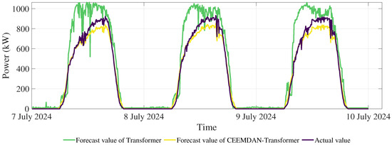
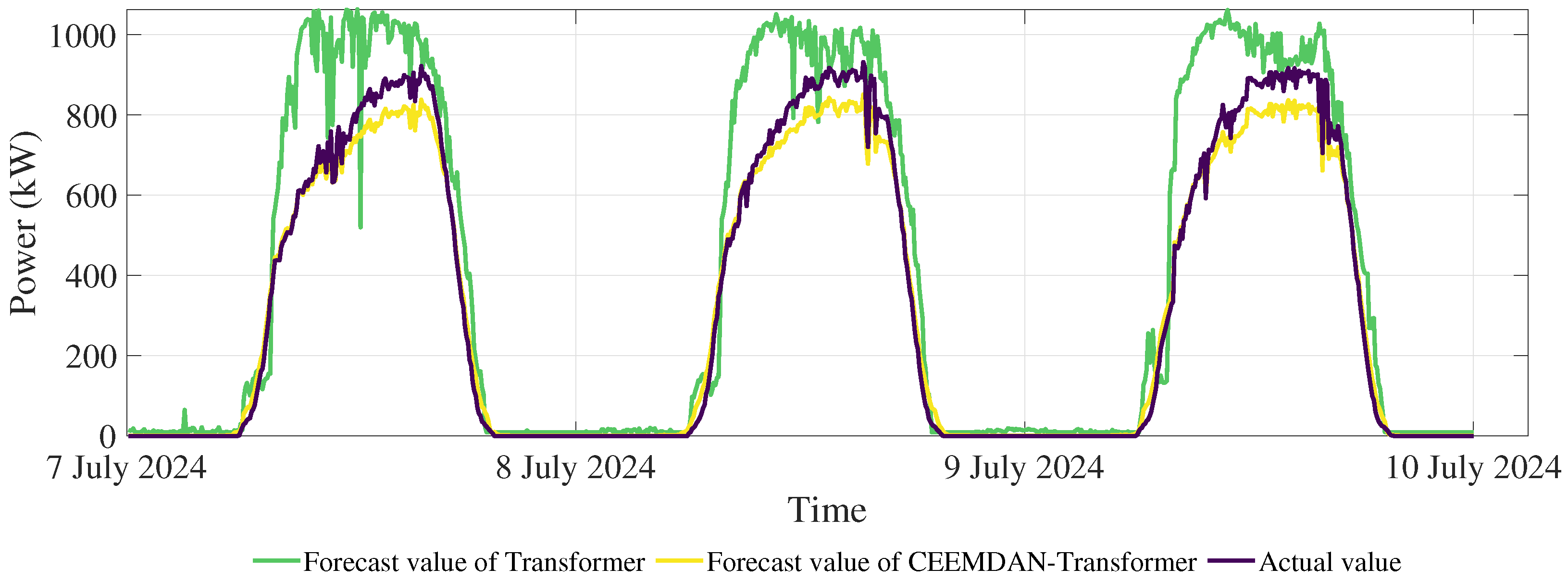
The clear-sky period from 7 to 9 July 2024 was selected for analysis. The power data under these conditions exhibits a relatively smooth curve, primarily governed by the deterministic physical laws of Earth’s rotation and the Sun–Earth relative position. As shown in Figure 7, the baseline Transformer model model can only roughly track the overall trend. Its errors mainly stem from the challenge of simultaneously fitting the primary trend and the weak high-frequency perturbations, leading to insufficient capture of the details in the diurnal cycle physical process.
Figure 7.
Forecast result of sunny day before and after the introduction of CEEMDAN.
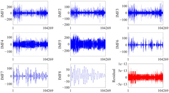
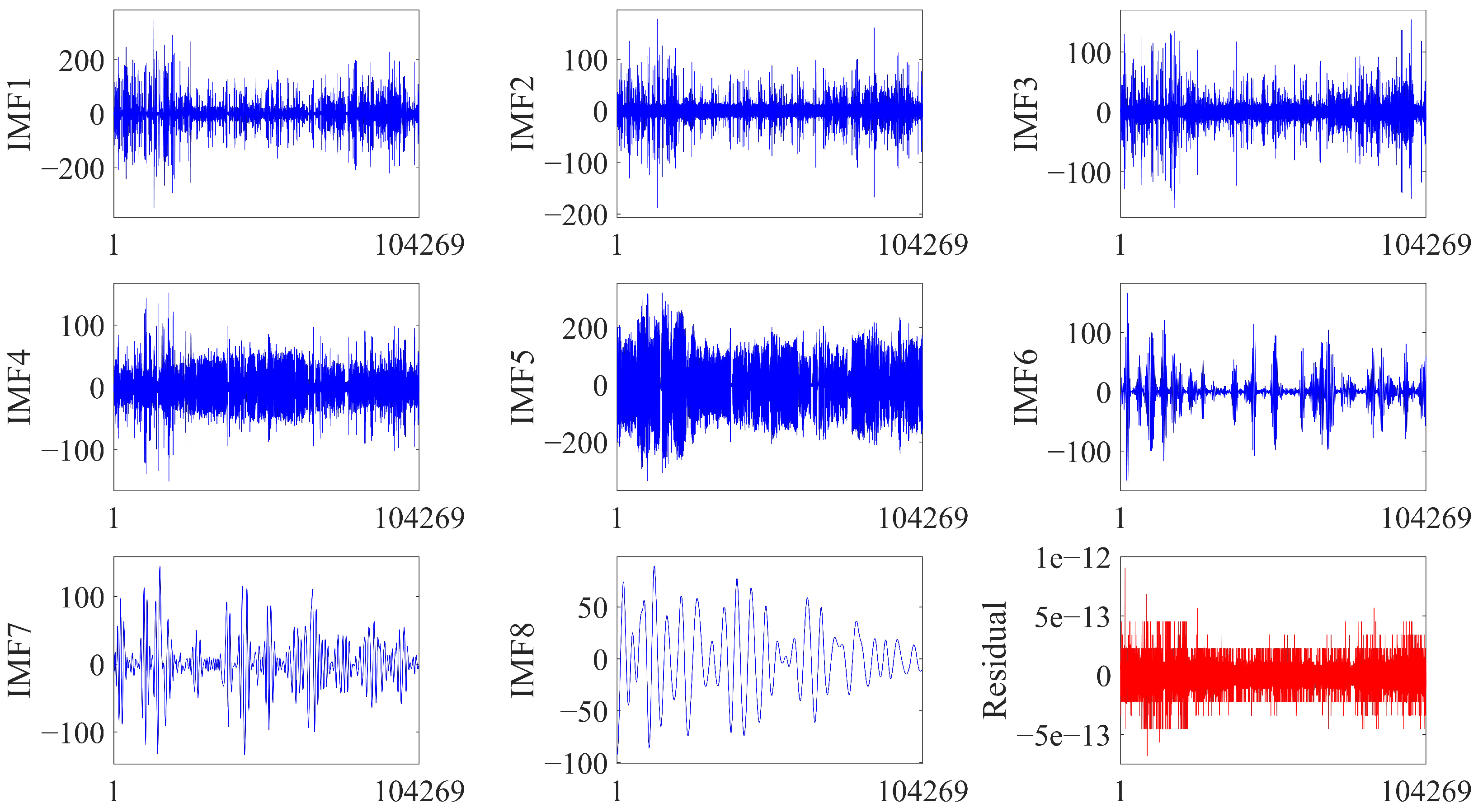
As shown in Table 3, the introduction of CEEMDAN yielded the most substantial performance improvement under clear-sky conditions, reducing the nRMSE from 43.447% to 8.419%. This is because CEEMDAN, acting as a physical fluctuation decoupler, successfully separated the mixed physical scales. The partial decomposition results from CEEMDAN are shown in Figure 8. This separation allows subsequent models to directly learn sub-signals with clearer physical meanings, thereby alleviating the challenge of modeling the original non-stationary signal directly, potentially facilitating a more effective learning process.
Figure 8.
Decomposition results of CEEMDAN.
4.2.2. Rainy Day
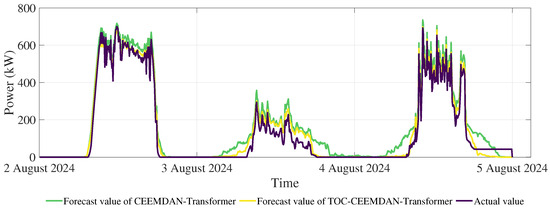
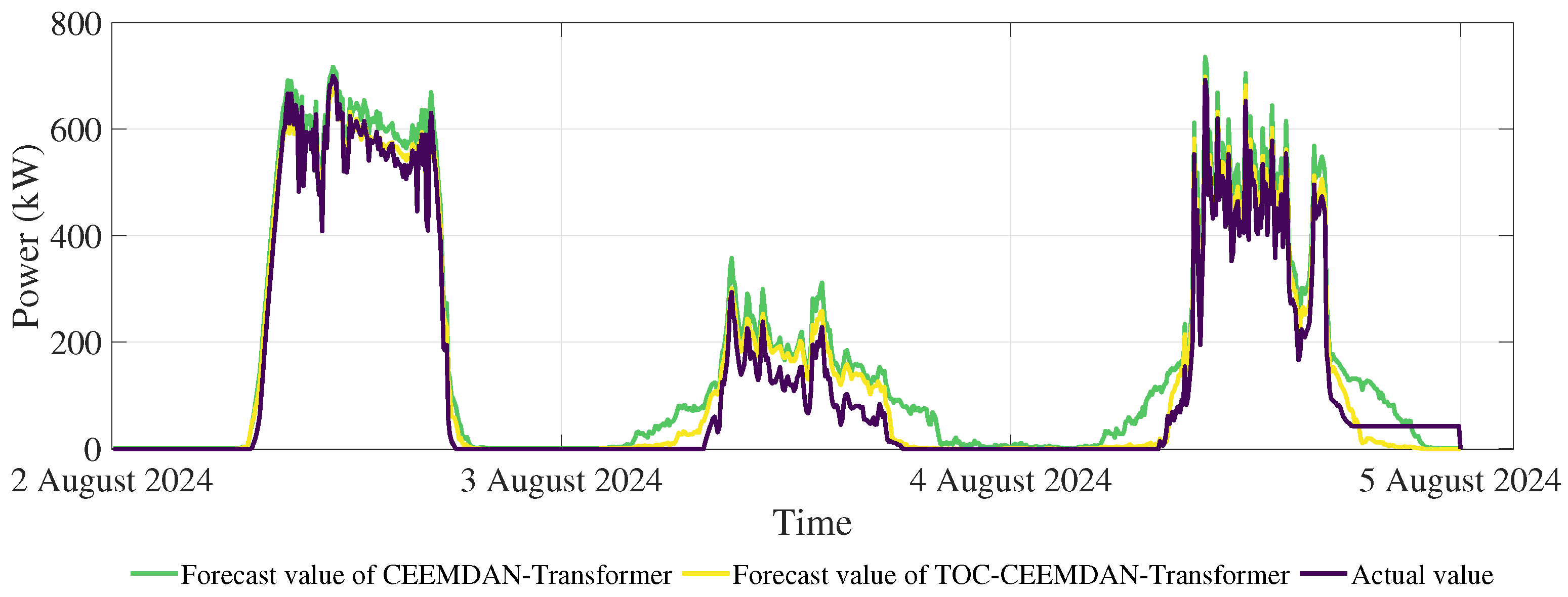
For the highly fluctuating rainy weather, the period from 2 to 4 August 2024 was selected as the sample. The core physical challenge in forecasting lies in capturing the dynamic physical process from cloud mass movement to radiation attenuation and subsequently to power drops.
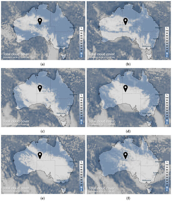
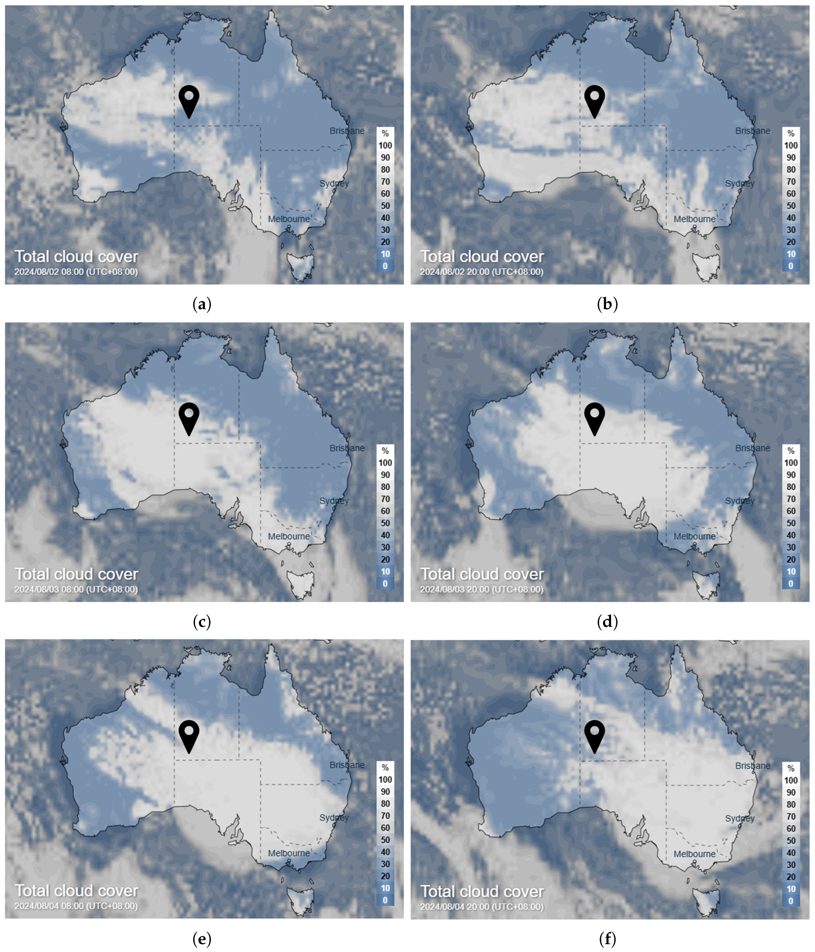
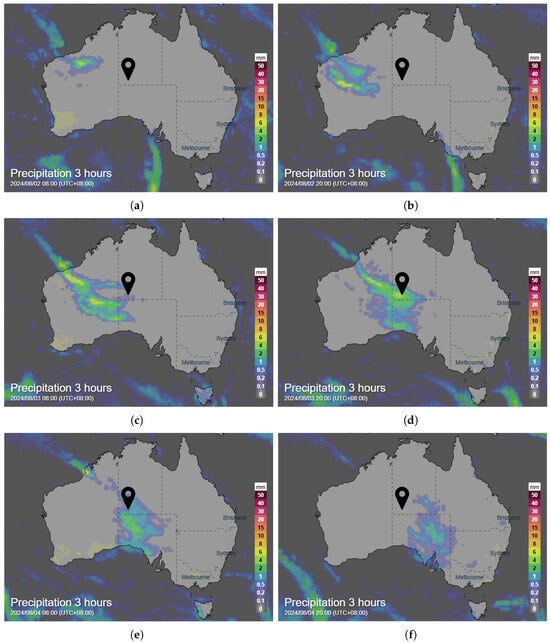
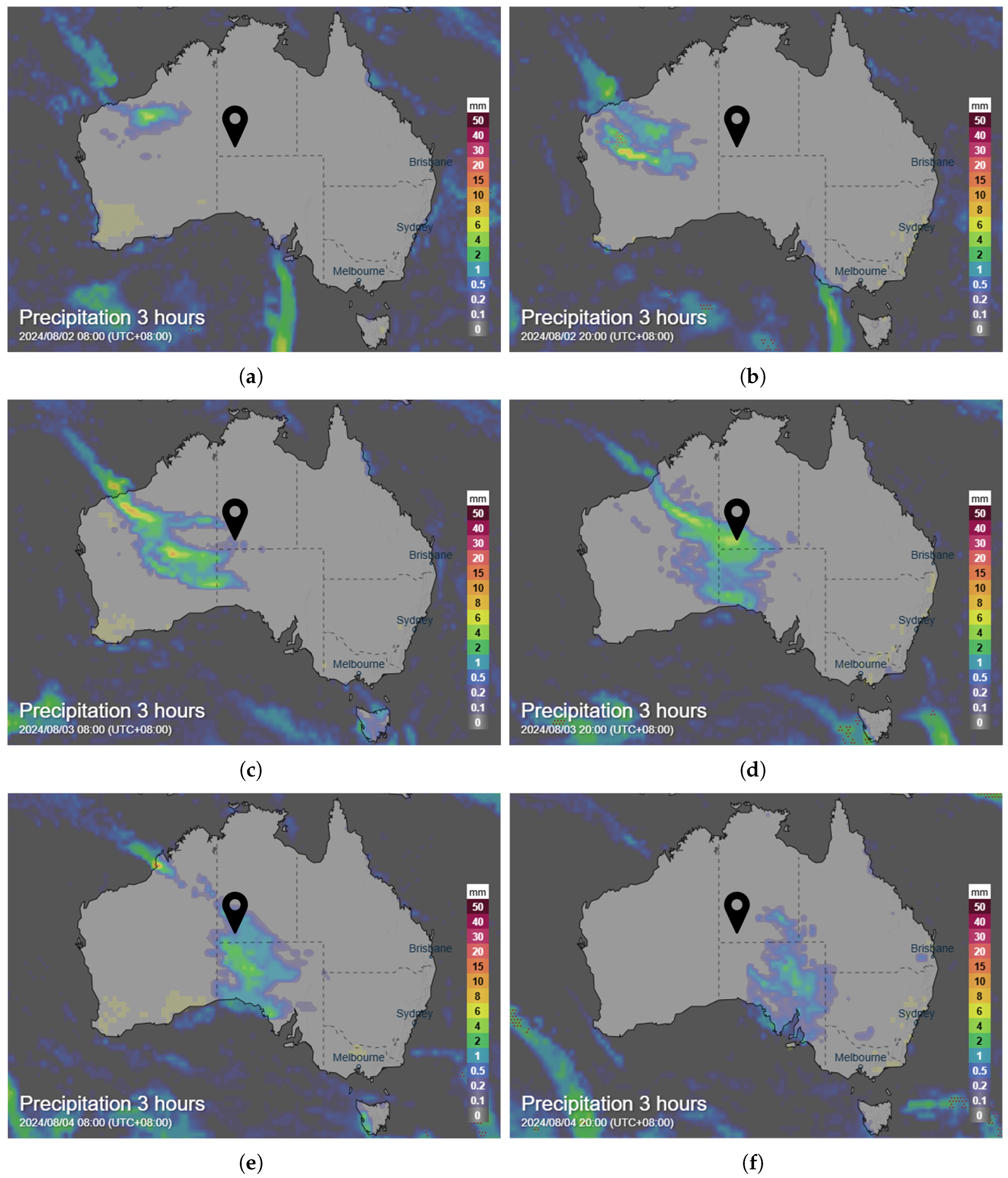
By integrating the total cloud cover and rainfall maps shown in Figure 9 and Figure 10, the physical reality of cloud clusters moving from the northwest through the Northern Territory towards the southeast is clearly observable from the cloud cover maps, along with its synchronous physical response on the power station’s output. On 2 August, the clouds had not yet fully covered the power station, resulting in moderate fluctuation intensity. According to the statistical rainfall maps, on 3 August, the rainfall band was directly above the power station accompanied by cloud cover, causing a sharp decrease in PV power and significant fluctuations. By 4 August, as the rainfall band and cloud clusters gradually moved away from the power station’s location, the complex movement patterns induced intense fluctuations in PV power. The original model responds inadequately to such rapidly changing physical forcings. The observed power fluctuations appear to correspond with cloud movement patterns, suggesting a potential relationship between cloud coverage and PV power output.
Figure 9.
Total cloud cover map of Australia from 2 to 4 August 2024: (a) 8:00 on 2 August 2024; (b) 20:00 on 2 August 2024; (c) 8:00 on 3 August 2024; (d) 20:00 on 3 August 2024; (e) 8:00 on 4 August 2024; (f) 20:00 on 4 August 2024. The black marker indicates the location of the Yulara power station.
Figure 10.
Rainfall map of Australia from 2 to 4 August 2024: (a) 8:00 on 2 August 2024; (b) 20:00 on 2 August 2024; (c) 8:00 on 3 August 2024; (d) 20:00 on 3 August 2024; (e) 8:00 on 4 August 2024; (f) 20:00 on 4 August 2024. The black marker indicates the location of the Yulara power station.
The performance improvement of the CEEMDAN–Transformer in this scenario was relatively limited, with its nRMSE even reaching 37.794%, slightly better than the baseline model. This might be because CEEMDAN, while removing noise, could also have smoothed or blurred the crucial, rapid, and localized abrupt edge features inherent in rainy weather—namely, the key information of sharp power drops and rises caused by rapidly moving clouds. The standard Transformer model hyperparameters might not have been optimally configured to recapture these attenuated rapid-change features from the decomposed components, which aligns with findings reported by researchers handling similar non-stationary signals [42]. It was only after introducing TOC for optimization that the model regained and enhanced its ability to capture this key physical process. Figure 11 shows the comparison of forecast curves for the radiation-dominated environment before and after introducing TOC. The TOC optimizer played an important role on rainy days, reducing the nRMSE from 37.794% (CEEMDAN–Transformer) to 20.768%, an improvement of approximately 46%. This confirms that TOC, acting as a physical mapping relationship optimizer, successfully identified the hyperparameter configuration that responds to the cloud–radiation influence.
Figure 11.
Forecast result of rainy day before and after the introduction of TOC.
4.2.3. Sandstorm Day
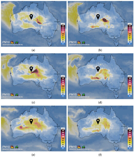
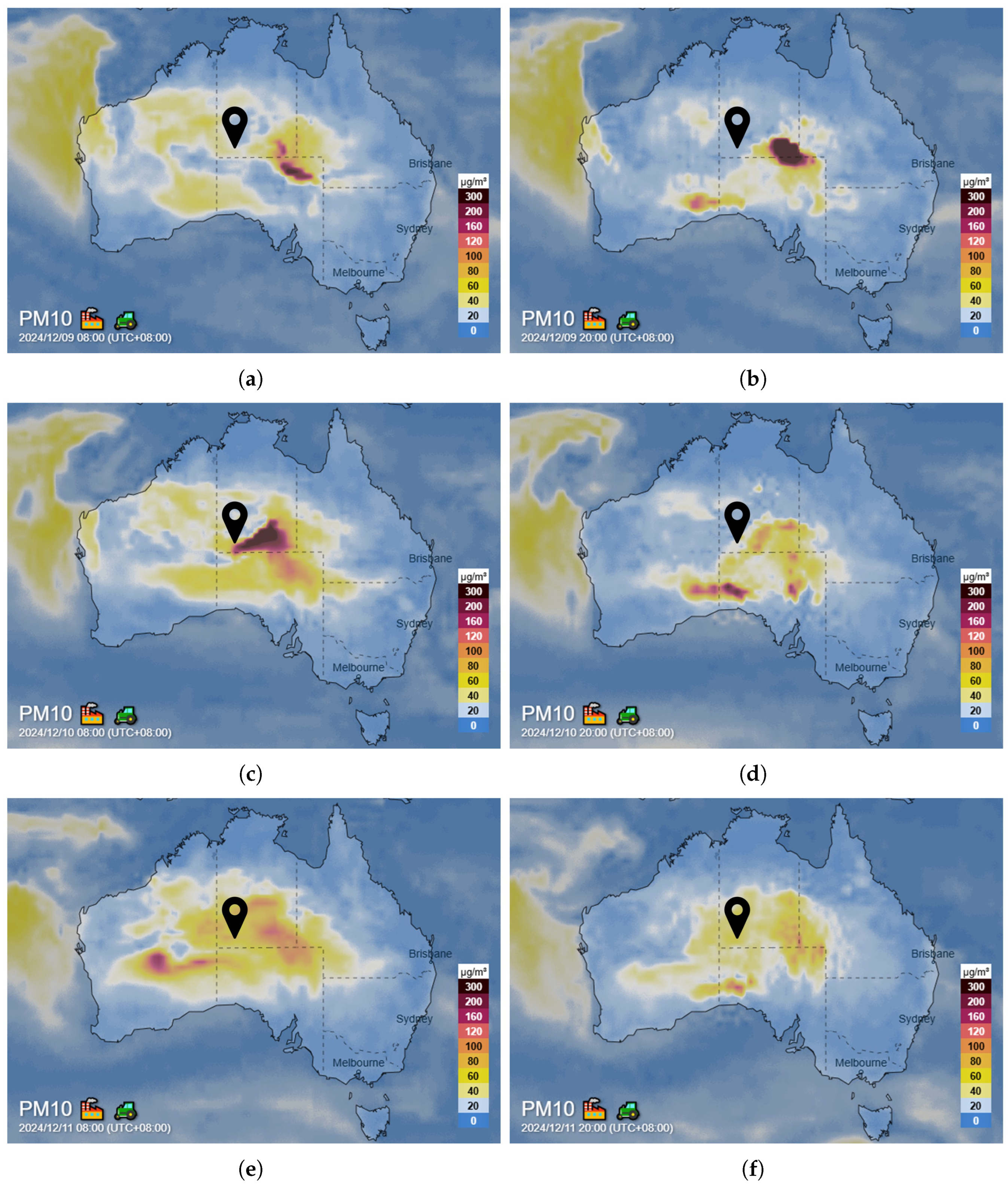
Dust storms represent another common type of non-stationary weather, epitomizing the most complex multi-field coupled physical environment. Highly nonlinear and intricate interactions exist among multiple physical variables such as dust, temperature, air pressure, and wind speed, posing challenges to the model’s learning capability [43]. PM10 concentration is a key indicator for measuring particulate matter levels in dust storm conditions. Figure 12 shows the local PM10 concentration maps from 9 December to 11 December.
Figure 12.
PM10 content map of Australia from 9 to 11 December 2024: (a) 8:00 on 9 December 2024; (b) 20:00 on 9 December 2024; (c) 8:00 on 10 December 2024; (d) 20:00 on 10 December 2024; (e) 8:00 on 11 December 2024; (f) 20:00 on 11 December 2024. The black marker indicates the location of the Yulara power station.
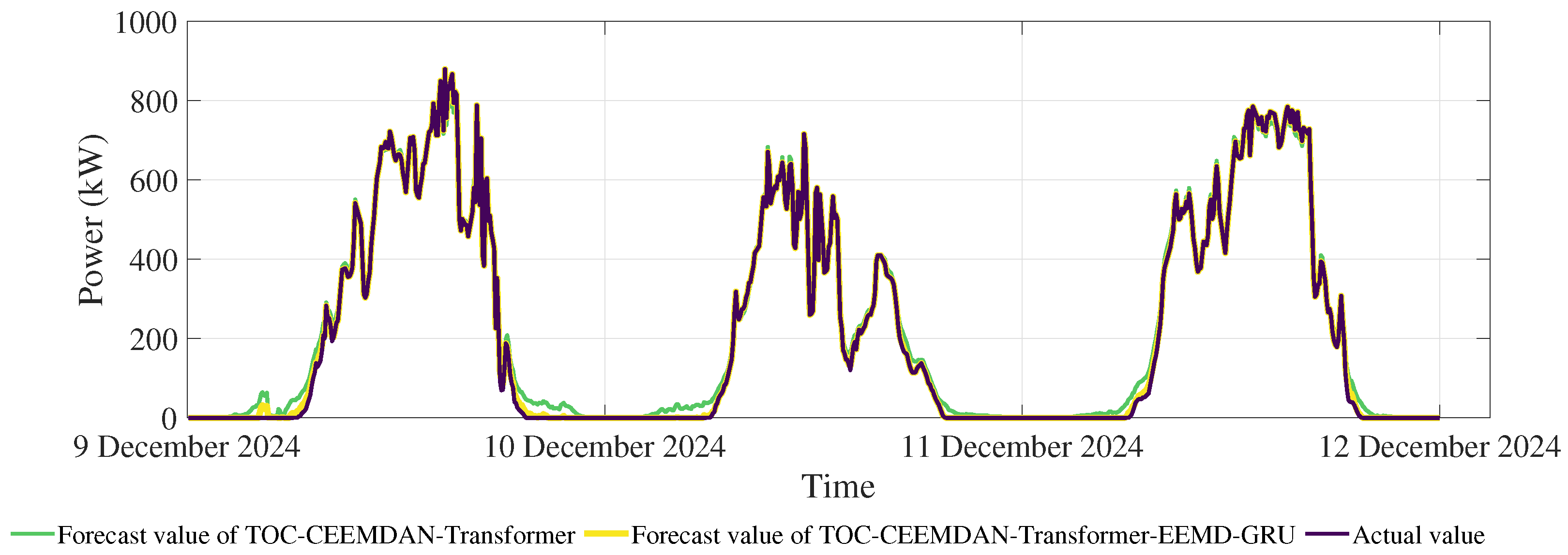
In this scenario, both CEEMDAN–Transformer and TOC–CEEMDAN–Transformer demonstrate relatively good performance, indicating that physical fluctuation decoupling and mapping relationship optimization positively contribute to handling such complex environments.
However, the introduction of the error correction module led to a substantial improvement, markedly reducing the nRMSE to 2.8069%. This indicates that when the main model faces the complex environment of nonlinear coupling among multiple physical fields like dust, temperature, and pressure, its learning capacity reaches its limit, resulting in systematic bias, as shown by the TOC–CEEMDAN–Transformer curve in Figure 13. Data in Table 3 show that the error correction module delivered performance improvements across all weather conditions. Under clear-sky conditions, this module reduced the nRMSE from 5.7241% to 1.0818%. This suggests that even for deterministic physical processes, the main model still exhibits subtle systematic biases, which the error correction module can effectively compensate for.
Figure 13.
Forecast result of sandstorm day before and after the introduction of Error Correction.
The complete model’s performance on dust storm days is even superior to that on rainy days. This does not imply that dust storms are easier to predict, but rather reveals the working mechanism of the error correction module: during dust storms, the main model, unable to fully decouple the complex coupling effects, produces regular systematic biases. These biases, acting as “unmodeled physical effects,” are accurately captured and learned by the error correction module. In contrast, the rapid and stochastic fluctuations of power during rainy days result in residual errors with weaker regularity, increasing the learning difficulty. This highlights the potential of hybrid models in addressing complex spatiotemporal dependency problems [44].
Through in-depth deconstruction of the performance metrics, the functional roles and operational boundaries of each module are clearly revealed. CEEMDAN decouples the mixed physical fluctuation modes, showing particularly significant improvement for deterministic processes; the TOC optimizer identifies globally optimal parameters adaptable to multi-modal physical mappings, proving crucial for responding to rapidly changing physical processes; the error correction module specifically compensates for the complex coupled physical effects that the main model fails to resolve, serving as the core component for achieving robustness. These four elements form a functionally complementary and organic whole, collectively endowing the framework with generalization capability to handle different meteorological physical mechanisms. The performance improvement observed after error correction indicates that the residual sequence contained learnable, systematic components. This outcome lends support to the practical utility of the additive correction approach in this specific application, as it allowed a secondary model to successfully identify and compensate for these patterns.
4.3. Cross-Year Generalization Capability Discussion
To evaluate the robustness of the proposed framework under different climatic backgrounds, a series of cross-year and cross-period forecasting experiments were conducted. These experiments were designed to explicitly address potential concerns regarding normalization consistency and performance generalization across temporal distribution shifts.
Given the critical importance of comparable metrics in cross-year analysis, all models were evaluated using Normalized Root Mean Square Error (nRMSE), calculated as a percentage of the mean actual power. This ensures a consistent and scale-invariant comparison across datasets from different years.
The experimental design incorporated multiple training-test splits, as detailed in Table 5, to provide a more comprehensive assessment than a single cross-year case. The results indicate that the proposed framework experiences a predictable and moderate performance degradation when applied to data from a different year or period, which is a typical characteristic of forecasting models facing natural distribution shifts.
Table 5.
Indicators on different year datasets. The suffix letter A indicates the first half of the year and the suffix letter B indicates the second half of the year.
For instance, when trained on data from the first half of 2024 (2024A) and tested on the first half of 2025 (2025A), the framework’s nRMSE was 13.4%. This represents a noticeable increase from the 4.68% nRMSE achieved on the within-year test set (2024B), but it is a realistic degradation given the interannual climatic variation. Crucially, this performance remains substantially better than that of baseline models under the same challenging cross-year conditions. The results of the cross-year validation show that the nRMSE values fluctuate between 4.68% and 15.88%, which provides preliminary evidence of the model’s temporal robustness.
To further address practical utility, we validated the annual total energy consistency between predicted and measured values over the test period. The relative error was calculated to be 2.56%, indicating that the framework maintains reasonable fidelity in predicting total energy output despite the point forecast error.
5. Conclusions
This study addresses the challenge of photovoltaic power forecasting under ENSO-driven climate transitions by proposing a modular four-stage framework. The research demonstrates that decomposing the forecasting task into specialized stages—fluctuation mode decoupling, mapping relationship optimization, spatiotemporal dependency learning, and residual error compensation—provides a structured approach to handle the distinct physical processes governing different weather regimes.
Experimental results on data from Australia’s Yulara power station indicate that the framework achieves competitive performance across sunny, rainy, and sandstorm conditions, with R2 values of 0.99981, 0.99782, and 0.99947, respectively. More importantly, the progressive improvement observed in ablation studies suggests that each stage contributes uniquely to the framework’s overall performance. The cross-year validation shows nRMSE values ranging from 4.68% to 15.88% across different temporal splits, providing preliminary evidence of temporal robustness. The energy consistency validation, with a relative error of 2.56% between predicted and measured total energy, further supports the framework’s practical utility.
The ablation study demonstrates the unique contribution of each module (CEEMDAN, TOC, EEMD-GRU) to the final performance from an architectural perspective. This evidence partially reflects the model’s robustness to component selection and can be regarded as a preliminary exploration of architectural sensitivity. Experiments replacing the core learner Transformer model with CNN-BiLSTM showed that the complete framework based on CNN-BiLSTM also achieved effective prediction, indicating that the performance improvement stems primarily from the climate-resilient architecture design itself, rather than from the fortuitous advantage of any specific algorithm. The cross-year forecasting test using data from other years further suggested the framework’s generalization capability.
This study confirms that a structured understanding of weather-dependent fluctuation patterns, coupled with a modular framework design, provides an effective pathway for constructing high-performance and climate-resilient forecasting models; however, while the framework demonstrates performance across diverse weather conditions, future work should include more extensive validation across multiple locations and time periods to further establish its generalizability under different climatic regimes. The modular architecture of the framework offers inherent adaptability: the CEEMDAN decomposition can handle non-stationarity inherent to various climate zones, the TOC optimizer can search for parameters robust to different meteorological regimes, and the error correction mechanism can compensate for location-specific biases. This suggests potential applicability to other regions affected by different weather extremes (e.g., snowfall, fog, or typhoons) and to emerging PV technologies, though such extension would require retraining with local data and potentially adjusting the decomposition parameters to match local fluctuation characteristics.
Regarding computational efficiency, the framework employs a strategic separation between offline and online phases. The most computationally intensive components—CEEMDAN decomposition and TOC hyperparameter optimization—are performed offline during model development. The deployed forecasting system requires only sequential forward passes through the pre-trained Transformer model and EEMD-GRU models, making it feasible for near-real-time operation at the 5 min resolution of our study; while suitable for operational forecasting, further optimization would be needed for ultra-fast control applications, which we identify as a direction for future work through model lightweighting and edge deployment strategies.
A limitation of this study is that the hyperparameter optimization module was instantiated with a single algorithm (TOC), which requires a comprehensive comparative analysis of various optimizers within this framework to provide more generalized guidance on their selection. In future, more rigorous statistical methodologies, such as cross-correlation analysis and Vector Autoregression (VAR) models, will be incorporated to more clearly establish the causal relationship between meteorological phenomena and PV power fluctuation, thereby further enhancing the model’s physical interpretability. Future work will focus on two aspects, first, migrating this framework to other climate zones and power stations of different scales to verify its broader universality; and second, investigating model lightweighting and edge deployment to empower real-time grid control and energy management with this adaptable intelligence at lower computational costs. More rigorous statistical methods will be incorporated, such as cross-correlation analysis and vector autoregression models, to better establish causal relationships between meteorological phenomena and PV power fluctuations; while the cross-year experiments provide initial evidence of the framework’s robustness, more extensive validation across multiple years and locations would be needed to firmly establish its generalization capabilities under diverse climatic conditions. It should be noted that the core of this study lies in designing a modular prediction architecture to systematically address the non-stationarity and multi-field coupling physical challenges of PV power during El Niño–Southern Oscillation (ENSO) transitions. Formal statistical significance tests and confidence interval calculations, such as the t-test for assessing differences between model performances, will be incorporated in future work to more rigorously quantify the model’s superiority. Furthermore, while the Residual Correction Module (EEMD-GRU) is intended to learn and correct the systematic biases of the main model (Transformer model), formal diagnostic analysis of the residual sequence (e.g., autocorrelation tests) has not yet been performed. This offers a valuable direction for further refining the error correction strategy.
Author Contributions
Conceptualization, X.W. and Z.L.; methodology, X.W. and Z.L.; software, X.W., X.D., W.Z. and J.L.; validation, X.W., Z.L., X.D., W.Z. and J.L.; formal analysis, X.W.; investigation, X.W., X.D., W.Z. and J.L.; resources, Z.L.; data curation, X.W., X.D., W.Z. and J.L.; writing—original draft preparation, X.W.; writing—review and editing, Z.L.; visualization, X.W., X.D., W.Z. and J.L.; supervision, Z.L.; project administration, Z.L.; funding acquisition, Z.L. All authors have read and agreed to the published version of the manuscript.
Funding
This research was funded by the Key Research and Development Program of Gansu Province—Industrial Project under Grant No. 25YFGF002, the Natural Science Foundation of Gansu Province No. 24JRRA241, the Key Entrusted Projects of Gansu Provincial Social Science Planning No. 2024ZD002, College Students’ Innovative Entrepreneurial Training Plan Program No. DC2510732CY0971.
Data Availability Statement
The data used in this study are publicly available from the Desert Knowledge Australia Solar Centre at https://dkasolarcentre.com.au/download/notes-on-the-data (accessed on 16 August 2025).
Conflicts of Interest
The authors declare no conflicts of interest.
Abbreviations
The following abbreviations are used in this manuscript:
| PV | Photovoltaic |
| ENSO | El Niño–Southern Oscillation |
| CEEMDAN | Complete Ensemble Empirical Mode Decomposition with Adaptive Noise |
| IMFs | Intrinsic Mode Functions |
| TOC | Tornado Optimizer with Coriolis force |
| EEMD | Ensemble Empirical Mode Decomposition |
| GRU | Gated Recurrent Unit |
| LSTM | Long Short-Term Memory |
| CNN | Convolutional Neural Network |
| BiLSTM | Bidirectional Long Short-Term Memory |
| RMSE | Root Mean Square Error |
| MAE | Mean Absolute Error |
| Coefficient of Determination | |
| GHI | Global Horizontal Irradiance |
| PM10 | Particulate Matter with a diameter of 10 μm or less |
Appendix A. Model Hyperparameter Configuration Details
Appendix A provides the complete hyperparameter configurations for all key components employed in the proposed forecasting framework. These parameters were utilized to obtain the experimental results presented in the main text and are crucial for the reproducibility of this study.
Table A1.
CEEMDAN decomposition parameters.
Table A2.
TOC optimization parameters.
Table A3.
Key parameters of the Transformer model network.
References
- Du, J.; Zheng, J.; Liang, Y.; Wang, B.; Klemeš, J.J.; Lu, X.; Tu, R.; Liao, Q.; Xu, N.; Xia, Y. A Knowledge-Enhanced Graph-Based Temporal-Spatial Network for Natural Gas Consumption Prediction. Energy 2023, 263, 125976. [Google Scholar] [CrossRef] [Scilit]
- Yousif, J.H.; Kazem, H.A. Prediction and Evaluation of Photovoltaic-Thermal Energy Systems Production Using Artificial Neural Network and Experimental Dataset. Case Stud. Therm. Eng. 2021, 27, 101297. [Google Scholar] [CrossRef] [Scilit]
- International Energy Agency. Renewables 2024; IEA: Paris, France, 2024. [Google Scholar]
- Xu, S. Research on Power Prediction Method for Photovoltaic Power Generation Based on PEEEMD-BiLSTM-XGboost. Adv. Appl. Math. 2023, 12, 5039–5049. [Google Scholar] [CrossRef]
- Shukla, A.; Pachauri, R.K.; Hussain, A.; Ali, A.; Khan, B. Comparative Analysis Dust Accumulation Impact on PV Performance Using Artificial Neural Network and Machine Learning Algorithms. Results Eng. 2025, 26, 105024. [Google Scholar] [CrossRef] [Scilit]
- Huang, A.T.; Gillett, Z.E.; Taschetto, A.S. Australian Rainfall Increases During Multi-Year La Niña. Geophys. Res. Lett. 2024, 51, e2023GL106939. [Google Scholar] [CrossRef] [Scilit]
- McGregor, S.; Gallant, A.; Van Rensch, P. Quantifying ENSOs Impact on Australia’s Regional Monthly Rainfall Risk. Geophys. Res. Lett. 2024, 51, e2023GL106298. [Google Scholar] [CrossRef] [Scilit]
- Di Leo, P.; Ciocia, A.; Malgaroli, G.; Spertino, F. Advancements and Challenges in Photovoltaic Power Forecasting: A Comprehensive Review. Energies 2025, 18, 2108. [Google Scholar] [CrossRef] [Scilit]
- Tian, J.; Ooka, R.; Lee, D. Multi-scale solar radiation and photovoltaic power forecasting with machine learning algorithms in urban environment: A state-of-the-art review. J. Clean. Prod. 2023, 426, 139040. [Google Scholar] [CrossRef] [Scilit]
- Hearst, M.; Dumais, S.; Osuna, E.; Platt, J.; Scholkopf, B. Support vector machines. IEEE Intell. Syst. Appl. 1998, 13, 18–28. [Google Scholar] [CrossRef] [Scilit]
- Breiman, L. Random Forests. Mach. Learn. 2001, 45, 5–32. [Google Scholar] [CrossRef] [Scilit]
- Singh, S.; Mohapatra, A. Repeated wavelet transform based ARIMA model for very short-term wind speed forecasting. Renew. Energy 2019, 136, 758–768. [Google Scholar] [CrossRef] [Scilit]
- Hochreiter, S.; Schmidhuber, J. Long Short-Term Memory. Neural Comput. 1997, 9, 1735–1780. [Google Scholar] [CrossRef] [Scilit] [PubMed]
- Lecun, Y.; Bottou, L. Gradient-based learning applied to document recognition. Proc. IEEE 1998, 86, 2278–2324. [Google Scholar] [CrossRef] [Scilit]
- Mirza, A.F.; Mansoor, M.; Usman, M.; Ling, Q. A comprehensive approach for PV wind forecasting by using a hyperparameter tuned GCVCNN-MRNN deep learning model. Energy 2023, 283, 129189. [Google Scholar] [CrossRef] [Scilit]
- Amiri, A.; Chouder, A.; Oudira, H.; Silvestre, S.; Kichou, S. Improving Photovoltaic Power Prediction: Insights through Computational Modeling and Feature Selection. Energies 2024, 17, 3078. [Google Scholar] [CrossRef] [Scilit]
- Li, J.; Luo, Y.; Yang, S.; Wei, S.; Huang, Q. A Review of Uncertainty Prediction Methods for Renewable Energy Power. High Volt. Eng. 2021, 47, 1144–1157. (In Chinese) [Google Scholar]
- Wu, Z.; Huang, N. Ensemble Empirical Mode Decomposition: A Noise-Assisted Data Analysis Method. Adv. Adapt. Data Anal. 2009, 1, 1–41. [Google Scholar] [CrossRef] [Scilit]
- Huang, J.; Yin, Y.; Tang, M.; Mei, F. Short-Term Photovoltaic Output Prediction Based on CEEMDAN and Improved LSTM. Low Volt. Appar. 2023, 36–43. (In Chinese) [Google Scholar] [CrossRef]
- Chi, H.; Jiang, H.; Zhao, Y. Photovoltaic power prediction model based on EMD-KPCA-GRU. In Proceedings of the 8th International Conference on Energy System, Electricity and Power; SPIE: Bellingham, WA, USA, 2024; Volume 13159, p. 1315908. [Google Scholar] [CrossRef] [Scilit]
- Mu, M.; Qin, B.; Dai, G. The predictability study of weather and climate events related to artificial intelligence models. Adv. Atmos. Sci. 2024, 41, 1005–1025. [Google Scholar] [CrossRef] [Scilit]
- Rchid, A.M.; Attia, M.; Mahmoud, M.E.M.; Aoulmi, Z.; Mahmoud, A.O. Solar photovoltaic power generation using machine learning considering weather conditions: A case study of Biret, Mauritania. Eng. Appl. Artif. Intell. 2025, 162, 112621. [Google Scholar] [CrossRef] [Scilit]
- Jiang, K.; Liu, N.; Wang, K.; Chen, Y.; Wang, J.; Liu, Y. Spatiotemporal assessment of renewable adequacy during diverse extreme weather events in China. Nat. Commun. 2025, 16, 5198. [Google Scholar] [CrossRef] [Scilit]
- Albani, A.; Ibrahim, M.Z.; Abdul Ghani, S.S.; Mat Rofi, M.Z.; Taslin, P.N.A. The Impact Study of El Niño-Southern Oscillation to the Wind and Solar Data in Malaysia Using the Wavelet Analysis. Front. Energy Res. 2021, 8, 591469. [Google Scholar] [CrossRef] [Scilit]
- Zhu, Y.; Zhang, R.H.; Wang, F.; Cai, W.; Li, D.; Guan, S.; Li, Y. Projection of ENSO using observation-informed deep learning. Nat. Commun. 2025, 16, 7736. [Google Scholar] [CrossRef] [Scilit]
- Geng, H. Photovoltaic Prediction Model Based on Covariance Matrix Adaptive Evolution Strategy and Error Correction. Master’s Thesis, Xi’an University of Technology, Xi’an, China, 2023. (In Chinese) [Google Scholar]
- Desert Knowledge Australia Solar Centre. Download Data, 2024. Location: Yulara Station. Available online: https://dkasolarcentre.com.au/download/notes-on-the-data (accessed on 24 August 2025).
- Trenberth, K.E. The Definition of El Niño. Bull. Am. Meteorol. Soc. 1997, 78, 2771–2778. [Google Scholar] [CrossRef] [Scilit]
- Iheanetu, K.J. Solar Photovoltaic Power Forecasting: A Review. Sustainability 2022, 14, 17005. [Google Scholar] [CrossRef] [Scilit]
- Iqbal, M. INDEX. In An Introduction to Solar Radiation; Academic Press: Toronto, ON, Canada, 1983; pp. 387–390. [Google Scholar] [CrossRef] [Scilit]
- Liou, K.N. An Introduction to Atmospheric Radiation; Academic Press: Cambridge, MA, USA, 2002. [Google Scholar]
- Shao, Y.; Wyrwoll, K.H.; Chappell, A.; Huang, J.; Lin, Z.; McTainsh, G.H.; Mikami, M.; Tanaka, T.Y.; Wang, X.; Yoon, S. Dust cycle: An emerging core theme in Earth system science. Aeolian Res. 2011, 2, 181–204. [Google Scholar] [CrossRef] [Scilit]
- Torres, M.E.; Colominas, M.A.; Schlotthauer, G.; Flandrin, P. A complete ensemble empirical mode decomposition with adaptive noise. In Proceedings of the IEEE International Conference on Acoustics, Speech and Signal Processing, Prague, Czech Republic, 22–27 May 2011; pp. 4144–4147. [Google Scholar] [CrossRef] [Scilit]
- Huang, N.E.; Shen, Z.; Long, S.R.; Wu, M.C.; Shih, H.H.; Zheng, Q.; Yen, N.C.; Tung, C.C.; Liu, H.H. The empirical mode decomposition and the Hilbert spectrum for nonlinear and non-stationary time series analysis. Proc. A 1998, 454, 903–995. [Google Scholar] [CrossRef] [Scilit]
- Braik, M.; Al-Hiary, H.; Alzoubi, H.; Hammouri, A.; Al-Betar, M.A.; Awadallah, M.A. Tornado optimizer with Coriolis force: A novel bio-inspired meta-heuristic algorithm for solving engineering problems. Artif. Intell. Rev. 2025, 58, 123. [Google Scholar] [CrossRef] [Scilit]
- Vaswani, A.; Shazeer, N.; Parmar, N.; Uszkoreit, J.; Jones, L.; Gomez, A.N.; Kaiser, L.; Polosukhin, I. Attention Is All You Need. arXiv 2017, arXiv:1706.03762. [Google Scholar] [CrossRef] [Scilit]
- Hyndman, R.; Athanasopoulos, G. Forecasting: Principles and Practice, 3rd ed.; OTexts: Melbourne, Australia, 2021. [Google Scholar]
- Chung, J.; Gulcehre, C.; Cho, K.; Bengio, Y. Empirical Evaluation of Gated Recurrent Neural Networks on Sequence Modeling. arXiv 2014, arXiv:1412.3555. [Google Scholar] [CrossRef] [Scilit]
- Zhang, S.; Zheng, D.; Hu, X.; Yang, M. Bidirectional Long Short-Term Memory Networks for Relation Classification. In Proceedings of the Pacific Asia Conference on Language, Information and Computation, Shanghai, China, 30 October–1 November 2015; pp. 73–78. [Google Scholar]
- Shalini, T.A.; Revathi, B.S. Power generation forecasting using deep learning CNN-based BILSTM technique for renewable energy systems. J. Intell. Fuzzy Syst. 2022, 43, 8247–8262. [Google Scholar] [CrossRef] [Scilit]
- Asghar, R.; Fulginei, F.R.; Quercio, M.; Maoz, M.; Sabino, L.; Abusara, M. Day-ahead photovoltaic power forecasting using a hybrid BiLSTM-CNN model. In Proceedings of the International Conference on Intelligent Computing in Data Sciences, Marrakech, Morocco, 23–24 October 2024; IEEE: Piscataway, NJ, USA, 2024; pp. 1–8. [Google Scholar]
- Su, Y.; Wang, Z.; Dong, Z.; Hua, X.; Ye, T.; Song, Z.; Shao, Y. Frequency-aware ultra-short-term wind power forecasting using CEEMDAN–VMD–SE and Transformer–GRU networks. Energy 2025, 338, 138715. [Google Scholar] [CrossRef] [Scilit]
- Li, X.; Niu, K. Effectively predict the solar radiation transmittance of dusty photovoltaic panels through Lambert-Beer law. Renew. Energy 2018, 123, 634–638. [Google Scholar] [CrossRef] [Scilit]
- He, S.; Liu, Y.; Peng, J.; Xu, D.; Wang, Y. A CEEMDAN-GNN-transformer hybrid model for air quality index forecasting: A case study of Chang’an town, Dongguan, China. Front. Environ. Sci. 2025, 13, 1653446. [Google Scholar] [CrossRef] [Scilit]

Disclaimer/Publisher’s Note: The statements, opinions and data contained in all publications are solely those of the individual author(s) and contributor(s) and not of MDPI and/or the editor(s). MDPI and/or the editor(s) disclaim responsibility for any injury to people or property resulting from any ideas, methods, instructions or products referred to in the content. |
© 2026 by the authors. Licensee MDPI, Basel, Switzerland. This article is an open access article distributed under the terms and conditions of the Creative Commons Attribution (CC BY) license.