Surrogate Modeling of a SOFC/GT Hybrid System Based on Extended State Observer Feature Extraction

Abstract

Solid oxide fuel cell (SOFC) and gas turbine (GT) hybrid systems exhibit inherent system uncertainties and unmodeled dynamics during operation, which compromise the accuracy of predicting gas turbine power. This poses challenges for system operation analysis and energy management. To enhance the prediction accuracy and stability of gas turbine power in SOFC/GT hybrid systems, a power prediction method capable of incorporating total system disturbance information is investigated. This study constructs a high-fidelity simulation model of an SOFC/GT hybrid system to generate gas turbine power prediction datasets. With fuel utilization (FU) as the input and gas turbine power as the output, this system is assumed to be a first-order dynamic system. Building upon this foundation, an extended state observer (ESO) is employed to extract the total system disturbance ($f$) that affects the power output of the gas turbine, excluding fuel utilization. The total disturbance $f$ and fuel utilization are used as inputs to a Backpropagation (BP) neural network to construct a disturbance-aware power prediction model. The predictive performance of the proposed method is evaluated by comparison with a BP neural network without disturbance estimation information and several benchmark models. Simulation results indicate that incorporating the disturbance term estimated by ESO enhances both the accuracy and stability of the BP neural network’s power prediction, particularly under operating conditions characterized by significant power fluctuations. Quantitatively, when comparing the predictive model with disturbance included to the model without disturbance, including the disturbance reduces the prediction error by approximately 89.33% (MSE) and 67.34% (RMSE), while the coefficient of determination R² increases by 0.1132, demonstrating a substantial improvement in predictive performance under the same test conditions. The research findings indicate that incorporating disturbance information into data-driven prediction models represents a viable modeling approach, providing effective support for predicting gas turbine power in SOFC/GT hybrid systems.

1. Introduction

In hybrid power systems, the accuracy of power prediction for each energy supply unit is crucial for the effective implementation of energy management strategies. If the output power prediction of the supply unit is inaccurate, it will directly lead to a reduction in the overall energy utilization efficiency of the integrated system.

The solid oxide fuel cell (SOFC) and gas turbine (GT) hybrid system combines an SOFC with a GT via thermodynamic and mass-flow coupling to jointly produce electricity [1]. Combining the complementary strengths of two highly efficient technologies enables the realization of cascading energy utilization.

SOFC/GT hybrid systems can be categorized into two types based on the relative positioning of the SOFC and GT: bottom-level cycle and top-level cycle [2]. In a top-level cycle, the fuel cell is installed upstream of the gas turbine combustion chamber in the SOFC/GT hybrid system. The exhaust gas from the SOFC reaction enters the GT combustion chamber for combustion, then flows into the turbine for expansion and power generation. The turbine generates electricity externally via the generator and provides power to the compressor. The top-level loop pressurized SOFC/GT hybrid system has garnered significant attention and application in distributed power generation, microgrids, marine propulsion, and large-scale transportation due to its high efficiency and low emissions.

In SOFC/GT hybrid systems, the load allocation strategy between the SOFC and GT is a key factor in maximizing overall system efficiency. In particular, SOFCs are relatively slow-responding power systems, whereas GTs react rapidly. When the system needs to respond to rapidly changing load demands, the power forecasting of the faster-responding GT system plays a crucial role in the proper implementation of energy management decisions. Predicting the output power of the gas turbine in advance can optimize the fuel utilization rate of the SOFC, coordinate the slow dynamics of the SOFC with the fast dynamics of the GT, and achieve smooth power output. Therefore, GT power prediction serves as one of the core inputs for system energy management, with its significance being particularly pronounced in multi-energy systems that integrate compressed air energy storage.

Recent studies have demonstrated that enhancing input features or augmenting training data can substantially improve the predictive performance of neural network models in time-series forecasting. Javeri et al. [3] showed that combining data augmentation with AutoML effectively reduces forecasting errors in time-series prediction tasks. Zhang et al. [4] reported that stabilizing input sequences through tailored data augmentation improves model generalization in runoff forecasting under highly variable conditions. Zhou et al. [5] demonstrated that data augmentation enables deep learning models to learn more robust features in scenarios with limited labeled data. These works highlight that augmenting or enriching the input space—whether by generating synthetic samples or extracting additional informative features—can enhance the learning capability and robustness of neural networks in a variety of forecasting scenarios. The current study’s use of additional disturbance features extracted via an Extended State Observer (ESO) as inputs to improve GT power prediction performance. In the field of dynamic systems with uncertainty and external disturbances, ESOs have been widely studied as an effective approach for estimating total disturbances and unmodeled dynamics. Pu et al. [6] proposed adaptive ESOs capable of accurately estimating aggregated disturbances in nonlinear systems with unknown uncertainties. Du et al. [7] further improved ESO designs to enhance robustness against measurement noise and disturbance variations. A comprehensive overview by Zhang et al. [8] systematically summarizes the recent progress in ESO theory, design methods, and applications, highlighting the ESO’s capability to estimate both system states and total disturbances—including unmodeled dynamics, internal and external uncertainties—across a wide range of uncertain systems.

With the advancement of neural networks, researchers have proposed various typical models, including the backpropagation (BP) neural network, convolutional neural network, recurrent neural network, and their improved variants. These models demonstrate excellent capabilities in feature extraction and nonlinear mapping in various tasks. However, due to issues such as complex network architecture, slow convergence during training, or strong dependence on data, certain limitations remain.

Among numerous neural network models, the primary reason for selecting the BP neural network lies in its low computational cost, simple structure, and controllable training process. Compared with deep models such as convolutional neural networks and recurrent neural networks, the parameter size of BP neural networks is smaller and the training process is more transparent. This makes it conducive to accurately observing the performance changes brought about by perturbation information under the same experimental conditions. This lightweight structure minimizes the influence introduced by the model itself, enabling us to more clearly observe the effect of the disturbance information $f$ provided by the extended state observer (ESO) on the prediction results. Meanwhile, the simplicity of BP neural networks facilitates model analysis, enhancing the interpretability and causal insight of the simulation results.

The contributions of this paper are as follows: A predictive structure combining an extended state observer with a BP neural network is proposed. The total disturbance $f$ estimated by the ESO is introduced as an additional input feature into the neural network, enabling the model to explicitly utilize the system disturbance information and thereby improving the prediction performance of the GT power. By comparing the prediction results of BP neural network models with and without the inclusion of “$f$”, a quantitative analysis was conducted on the role of perturbation information in enhancing prediction accuracy and the coefficient of determination.

The remainder of this paper is organized as follows. Section 2 introduces the methodology employed herein, including the extended state observer and the backpropagation neural network model, and presents the proposed forecasting framework. Section 3 describes the construction of a simulation model for the SOFC/GT system and validation of the model’s effectiveness. Section 4 details the evaluation of the performance of the proposed method based on simulation data and comparative analysis with several benchmark prediction models. Finally, Section 5 summarises the work undertaken throughout the study.

2. Methodology

2.1. Extended State Observer

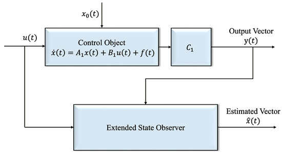
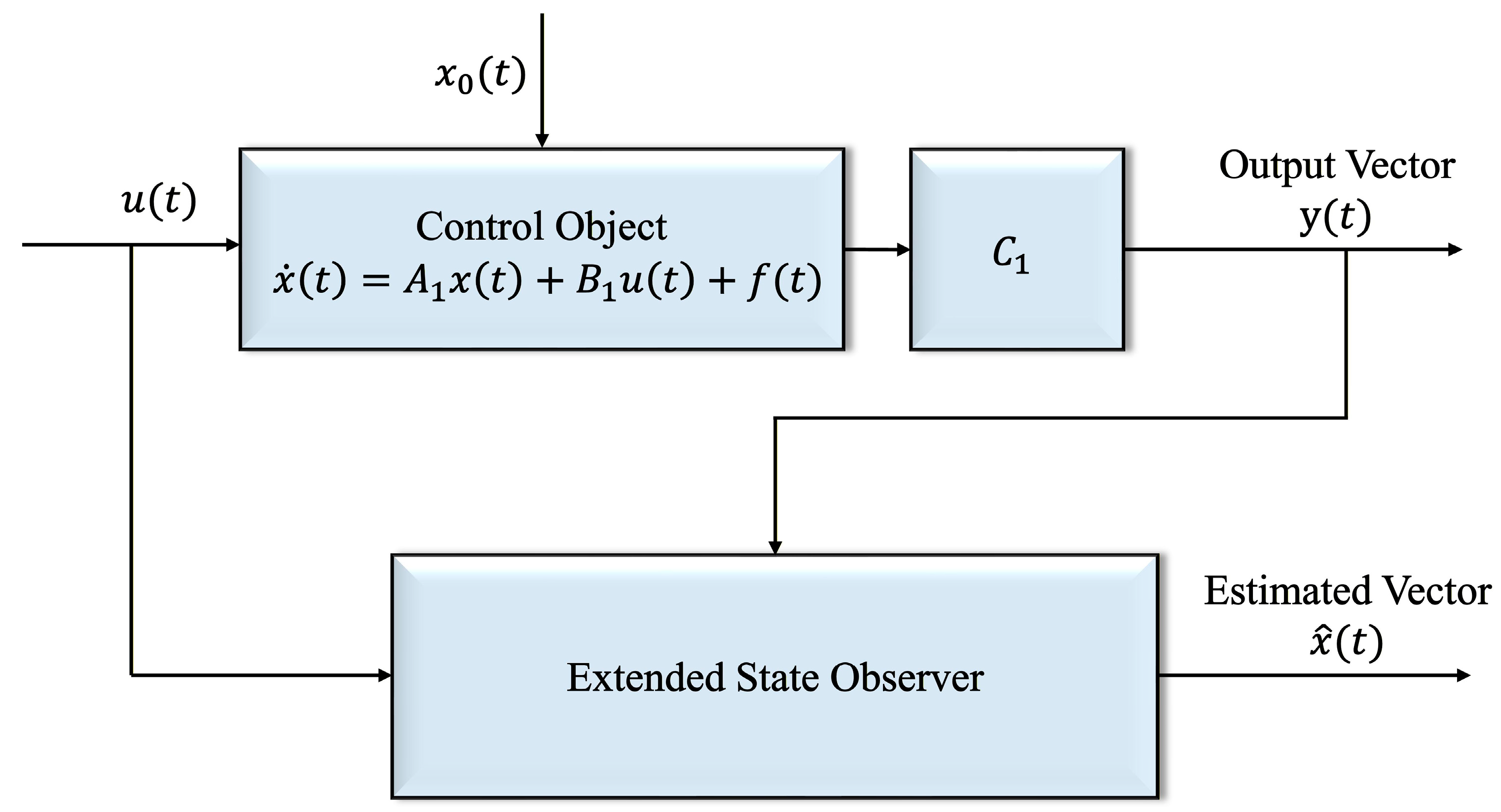
The ESO is a tool for dynamic system control and state estimation. Its core concept involves treating unknown disturbances or modeling errors within a system as an “extended state” and estimating it in real time through the observer [9]. To address the issue of the insufficient capture of disturbance information in power forecasting by traditional data-driven methods, this paper introduces an extended state observer. Figure 1 shows the schematic diagram of the ESO. ESO isolates unknown disturbances from complex system dynamics and provides auxiliary information for controllers or predictive models. In data-driven methods, ESO can reduce the impact of disturbances on predictions and enhance the model’s adaptability to non-stationary, nonlinear systems.

Figure 1. Schematic Diagram of ESO.

A system with fuel utilization rate as input and gas turbine power as output constitutes a first-order dynamic system, whose state-space model is expressed as

$$\left\{\begin{array}{l}\dot{x}\left(t\right)=A_{1}x\left(t\right)+B_{1}u\left(t\right)+f\left(t\right)\\ y\left(t\right)=C_{1}x\left(t\right)\end{array}\right.$$

(1)

Here, $x\left(t\right)\in R^n$ is the state variable; $u\left(t\right)\in R^p$ is the control input fuel utilization rate; $y\left(t\right)\in R^m$ is the output power of the system gas turbine; $f\left(t\right)$ represents the total disturbance term in the system.

The ESO captures the total disturbance acting on the system output, representing all unmodeled dynamics and external/internal perturbations. This total disturbance encompasses unmodeled dynamics, such as nonlinearities, couplings, and delays, as well as external and internal perturbations, including variations in operating conditions, load fluctuations, and component aging. In essence, the total disturbance acts as a consolidated variable capturing all effects on the system output not directly accounted for by the nominal model. By incorporating this term as an additional feature in the predictive model, the neural network can implicitly account for these unknown or unmodeled effects, thereby improving prediction accuracy and robustness.

In the formula,

$$A_1=\left[\begin{array}{cc}0& 1\\ 0& 0\end{array}\right], { B}_1=\left[{\displaystyle \genfrac{}{}{0pt}{}{b}{0}}\right], { C}_1=\left[\begin{array}{cc}1& 0\end{array}\right]$$

(2)

To achieve online estimation of the total disturbance to the system, an extended state observer is introduced. The disturbance term $f\left(t\right)$ is incorporated into the system model as an extended state, with the extended state variable defined as

$$x_1\left(t\right)=x\left(t\right), { x}_2\left(t\right)=f\left(t\right)$$

(3)

The total disturbance $f\left(t\right)$ is assumed to be differentiable with a bounded time derivative. Assuming that the perturbation term exhibits slow scaling changes on short timescales and has a bounded rate of change, i.e.,

$${\dot{x}}_2\left(t\right)\approx 0$$

(4)

Based on this, an extended second-order system model can be constructed as follows:

$$\left\{\begin{array}{l}{\dot{x}}_1\left(t\right)=A_1{x}_1\left(t\right)+B_{1}u\left(t\right)+x_2\left(t\right)\\ {\dot{x}}_2\left(t\right)=0\\ y\left(t\right)=C_1{x}_1\left(t\right)\end{array}\right.$$

(5)

According to Equation (1), the extended state observer [10,11] of the system can be expressed as

$$\left\{\begin{array}{l}{\dot{\widehat{x}}}_1\left(t\right)=A_1{\widehat{x}}_1\left(t\right)+B_{1}u\left(t\right)+{\widehat{x}}_2\left(t\right)+{\beta }_1(y\left(t\right)-C_1{\widehat{x}}_1(t))\\ {\dot{\widehat{x}}}_2\left(t\right)={\beta }_2(y\left(t\right)-{ C}_1{\widehat{x}}_1(t))\end{array}\right.$$

(6)

Here, ${\widehat{x}}_1(t)$ and ${\widehat{x}}_2\left(t\right)$ represent the estimated values of the system state and total disturbance, respectively, while ${\beta }_1$ and ${\beta }_2$ denote the observer gain parameters.

The state estimation error is defined as

$$e_1\left(t\right)=x_1\left(t\right)-{\widehat{x}}_1\left(t\right), { e}_2\left(t\right)=x_2\left(t\right)-{\widehat{x}}_2\left(t\right)$$

(7)

ESO possesses extremely strong stability and was first proposed by J. Han [12]. This method has been widely applied in the field of control engineering.

2.2. BP Feedforward Neural Network and Its Functions

The BP neural network is a typical type of artificial neural network model, with a network structure typically comprising an input layer, one or more hidden layers, and an output layer [13]. Each layer of neurons is fully connected to the previous layer, transmitting information through weighted summation and nonlinear activation functions. Network training employs the backpropagation algorithm to iteratively update weights by minimizing prediction errors, thereby achieving a nonlinear mapping between inputs and outputs.

In this study, the function of the BP neural network is to input the features processed by ESO into the network, predict the actual power output of the gas turbine, and thereby achieve accurate modeling and performance estimation of the system state.

In gas turbine power prediction tasks, system outputs are influenced not only by multiple input factors such as gas flow rate, ambient temperature, and pressure, but also by uncertainties including modeling errors, measurement noise, and external disturbances. Traditional BP neural networks can learn nonlinear relationships between inputs and outputs, but their predictive accuracy and stability are often constrained when complex disturbances or system non-stationarity are present. To better understand the strengths and weaknesses of existing neural network models, a comparison is provided in Table 1. Therefore, ESO was combined with the BP neural network to construct a hybrid prediction model. The ESO module extracts the total disturbance term $f$ from system inputs and outputs, using it as an auxiliary input for the BP neural network. This enhances the neural network’s sensitivity to disturbance characteristics and improves the model’s predictive performance under complex operating conditions.

Table 1. Advantages and Disadvantages of Each Model and Typical Applications.

Neural Network Models	Advantages	Disadvantages	Typical Applications
BP Neural Network	Theoretical maturity [14], achieves simplicity [15].	Prone to getting stuck in local minima [16], poor generalizability [17].	Forecast [18], function fitting [19].
Convolutional Neural Network (CNN)	Local feature extraction yields good results [20].	Multiple parameters [21], high computational load [22].	Image recognition [23].
Recurrent Neural Network (RNN)	Strong sequence processing capability [24].	Long-dependency problem [25].	Natural language processing [26], speech recognition [27].
Graph Neural Network	Strong communication skills [28], inductive data analysis capability [29].	Sensitive to image quality [30].	Social network analysis [31], transportation network and time-space prediction [32], financial network [33]
Transformer	Good parallelism [34], high performance [35].	Requires big data training [36].	Natural language processing [37], speech processing [38].

2.3. The Presented Model

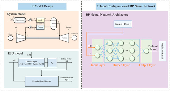
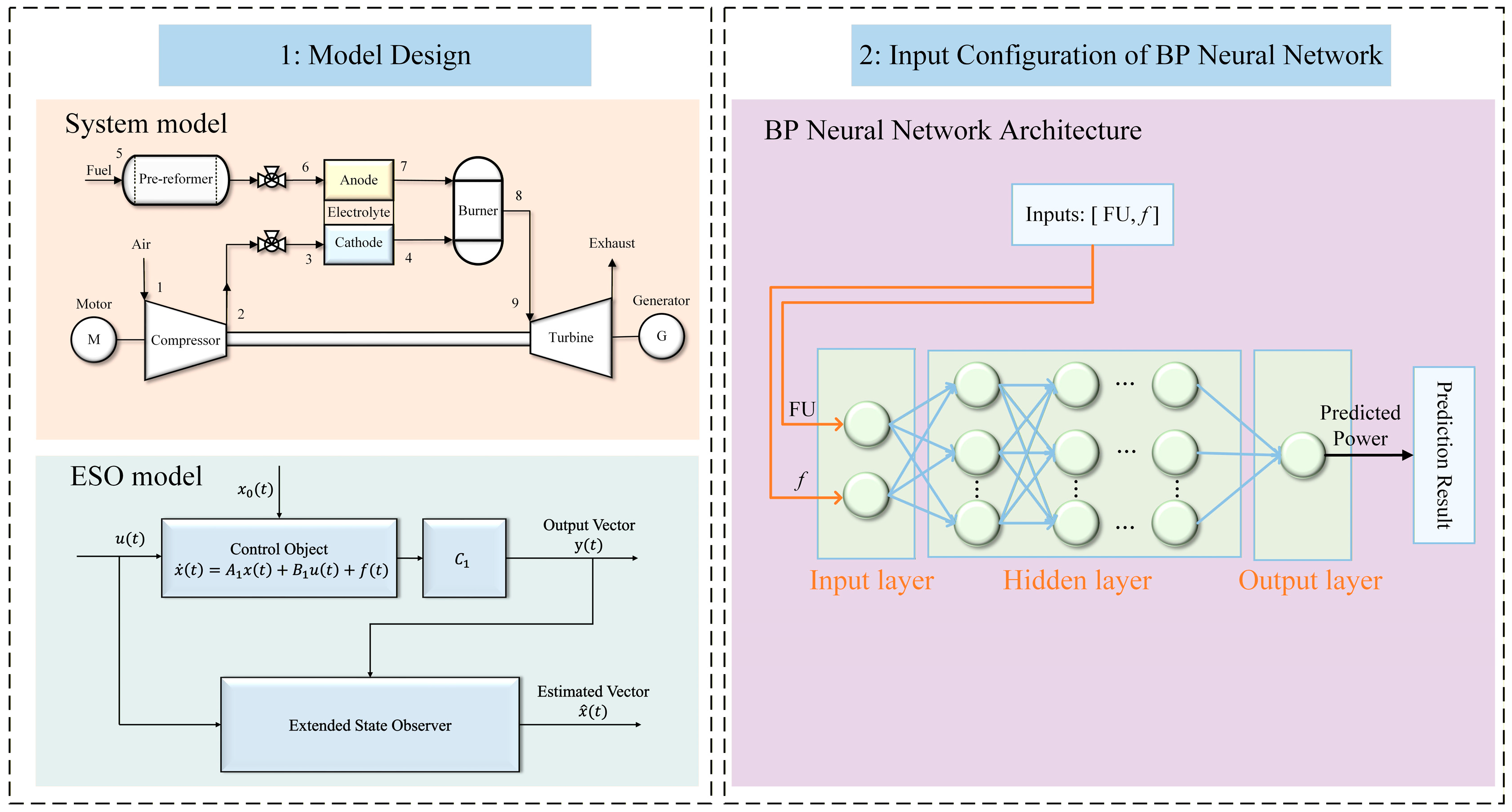
Figure 2 presents the proposed SOFC/GT top-level cycle system architecture, along with the corresponding ESO model and BP neural network structure. The SOFC/GT top-level cycle system describes the energy conversion and power output processes under various operating conditions. These processes are primarily used to generate system operational data, providing a data foundation for subsequent power forecasting. Based on the generated data, an extended state observer is established to analyze system dynamics. Unmodeled dynamics within the system and external disturbances are uniformly represented as disturbance terms, enabling the estimation and extraction of disturbance term $f$. The perturbation information obtained from ESO serves as a characteristic parameter reflecting system uncertainty, providing supplementary information for data-driven models.

Figure 2. ESO-BP Power Forecasting Framework Diagram.

A BP neural network model that takes the system input fuel utilization (FU) and the disturbance term $f$ extracted by ESO as inputs was constructed to achieve GT power prediction. Compared to prediction methods that rely solely on raw input variables, incorporating the perturbation feature $f$ enhances the model’s ability to characterize complex dynamic characteristics and uncertainties, thereby improving power forecasting accuracy.

3. Construction of SOFC/GT System Simulation Model

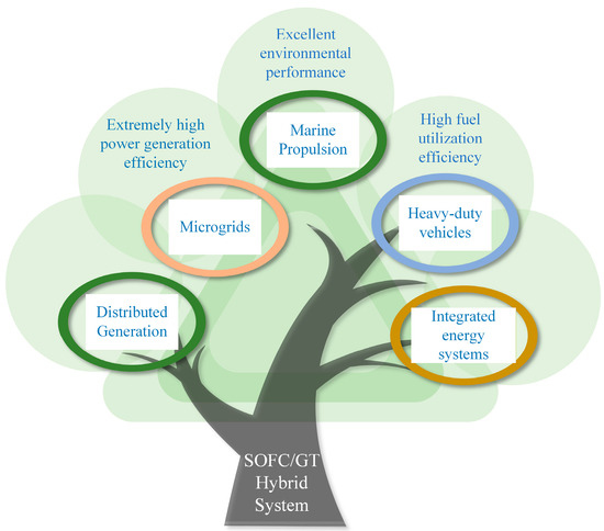
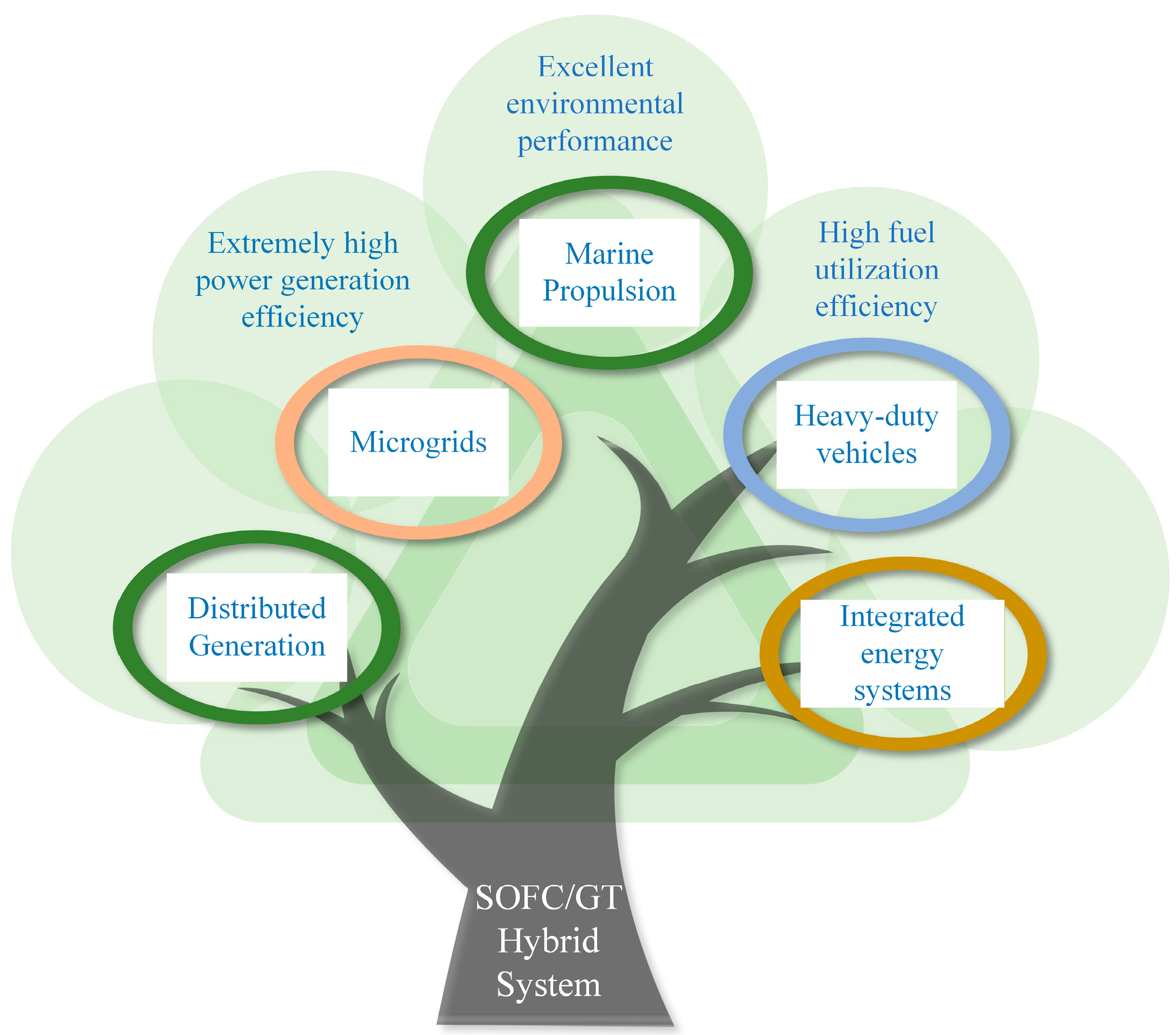
SOFC/GT hybrid systems can be applied in a variety of scenarios, including marine propulsion, microgrids, heavy-duty vehicles, distributed generation, and integrated energy systems, as illustrated in Figure 3. This figure highlights the typical application areas considered in the present study, providing context for the system modeling.

Figure 3. The application fields of the SOFC/GT hybrid system.

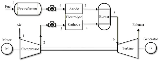
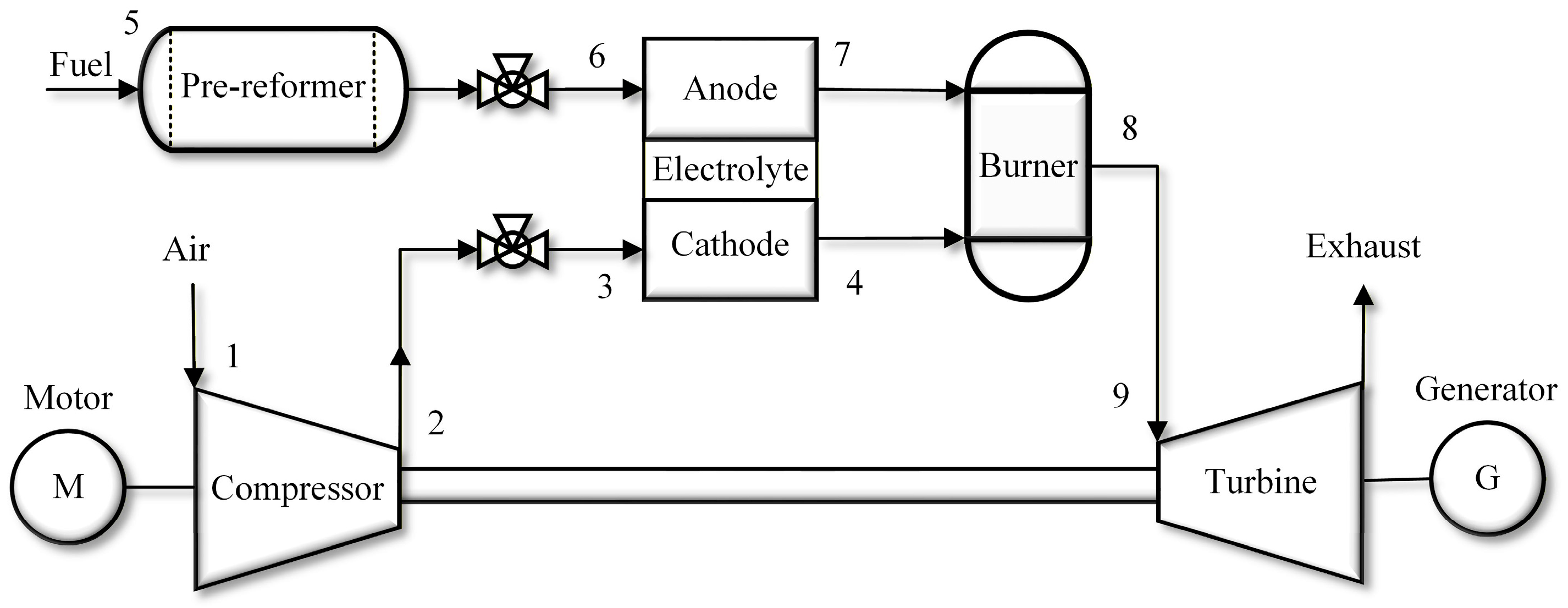
Building upon these application scenarios, the SOFC/GT system is composed of a solid oxide fuel cell subsystem and a gas turbine subsystem, which are coupled through energy and material flows [39]. Figure 4 shows the top-level cycle structure diagram of the SOFC/GT hybrid system. SOFCs directly convert chemical energy into electrical energy. Their exhaust gases possess high temperatures, which can further drive gas turbines to generate mechanical power, thereby enhancing the overall efficiency of the system’s energy utilization [40]. To achieve system simulation, this study employs mathematical modeling of the SOFC and GT subsystems based on the principles of energy conservation, mass conservation, and thermodynamic equilibrium. A coupled simulation model is formed by integrating heat flow with gas flow. The operating conditions of the SOFC/GT hybrid power generation system are summarized in Table 2.

Figure 4. Top-Level Cycle Diagram of the SOFC/GT Hybrid System. The numbered arrows (1–9) indicate information and material flows: (1) air from the compressor, (2) compressed air to the cathode, (3) auxiliary air flow, (4) cathode exhaust to the burner, (5) fuel to the pre-reformer, (6) reformed fuel to the anode, (7) anode exhaust to the burner, (8) burner exhaust to the turbine, (9) turbine output to the generator and exhaust.

Table 2. Operating conditions of the SOFC/GT hybrid power generation system.

Variable	Unit	Value
Fuel Import Composition	—	$100\% {\mathrm{C}\mathrm{H}}_4$
Fuel import flow	${\mathrm{m}\mathrm{o}\mathrm{l}·\mathrm{s}}^{-1}$	0.467
Air inlet composition	—	$79.99\% {\mathrm{N}}_2$ + $21.01\% {\mathrm{O}}_2$
Air inlet flow	${\mathrm{m}\mathrm{o}\mathrm{l}·\mathrm{s}}^{-1}$	20.211
Fuel Inlet Pressure	Pa	$1.013\times {10}^5$
Air inlet pressure	Pa	$1.013\times {10}^5$
Fuel inlet temperature	K	298
Air inlet temperature	K	298
Steam/carbon molar ratio	—	2.5
SOFC Current	A	267

3.1. SOFC Subsystem Model

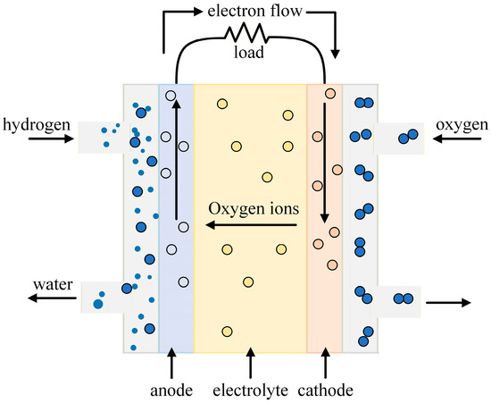
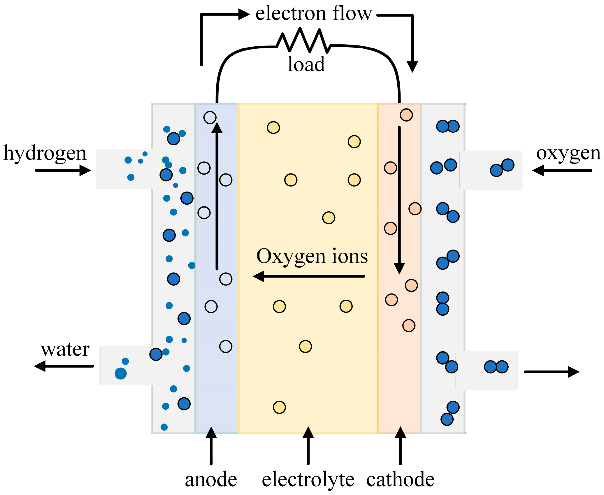
Within the SOFC/GT system, the SOFC operates as the main energy conversion component, producing electrical power from fuel electrochemical reactions while supplying high-temperature exhaust to the gas turbine [41]. Figure 5 illustrates the operating principle of the SOFC.

Figure 5. Operation principle of SOFC.

In developing the SOFC model, the stack is assumed to operate under steady-state conditions with one-dimensional, fully mixed gas flow, where polarization losses include activation, ohmic, and concentration components, and heat transfer losses within the stack are neglected.

The open-circuit voltage of the SOFC can be determined using the Nernst equation:

$$E_{Nernst}=E^0+{\displaystyle \frac{RT}{2F}}In\left({\displaystyle \frac{P_{H_2}{p}_{O_2}^{\frac{1}{2}}}{p_{H_{2}O}}}\right)$$

(8)

The actual output voltage after accounting for polarization loss is:

$$U_{sofc}=E_{Nernst}-{\eta }_{act}-{\eta }_{ohm}-{\eta }_{conc}$$

(9)

The output power of the SOFC is:

$$P_{sofc}=U_{sofc}\times I$$

(10)

Here, $E^0$ is the standard reversible voltage (V), $R$ is the gas constant ($\mathrm{J}·{\mathrm{m}\mathrm{o}\mathrm{l}}^{-1}·{\mathrm{K}}^{-1}$), $T$ is the absolute temperature (K), $F$ is Faraday’s constant ($\mathrm{C}·{\mathrm{m}\mathrm{o}\mathrm{l}}^{-1}$), $I$ is the stack current (A), and $p_{H_2}$, $p_{O_2}$, and $p_{H_{2}O}$ are the partial pressure of hydrogen, oxygen, and water vapor, respectively (Pa), ${\eta }_{act}$, ${\eta }_{ohm}$, and ${\eta }_{conc}$ denote the activation, ohmic, and concentration polarization losses, respectively (V).

Fuel utilization rate $U_f$ is defined as

$$U_f={\displaystyle \frac{{\dot{n}}_{H_{2,reacted}}}{{\dot{n}}_{H_{2,in}}}}$$

(11)

Among these, ${\dot{n}}_{H_{2,reacted}}$ represents the molar flow rate of hydrogen actually participating in the reaction ($\mathrm{m}\mathrm{o}\mathrm{l}·{\mathrm{s}}^{-1}$), while ${\dot{n}}_{H_{2,in}}$ denotes the molar flow rate of hydrogen entering the SOFC anode ($\mathrm{m}\mathrm{o}\mathrm{l}·{\mathrm{s}}^{-1}$). According to Faraday’s law, the relationship between hydrogen consumption and stack current $I$ is given by:

$${\dot{n}}_{H_{2,reacted}}={\displaystyle \frac{I}{2F}}$$

(12)

Therefore, fuel utilization efficiency can be further expressed as

$$U_f={\displaystyle \frac{I}{2F{\dot{n}}_{H_{2,in}}}}$$

(13)

Fuel utilization reflects the degree of fuel conversion in electrochemical reactions, typically controlled between 0.7 and 0.9 to balance efficiency and stability.

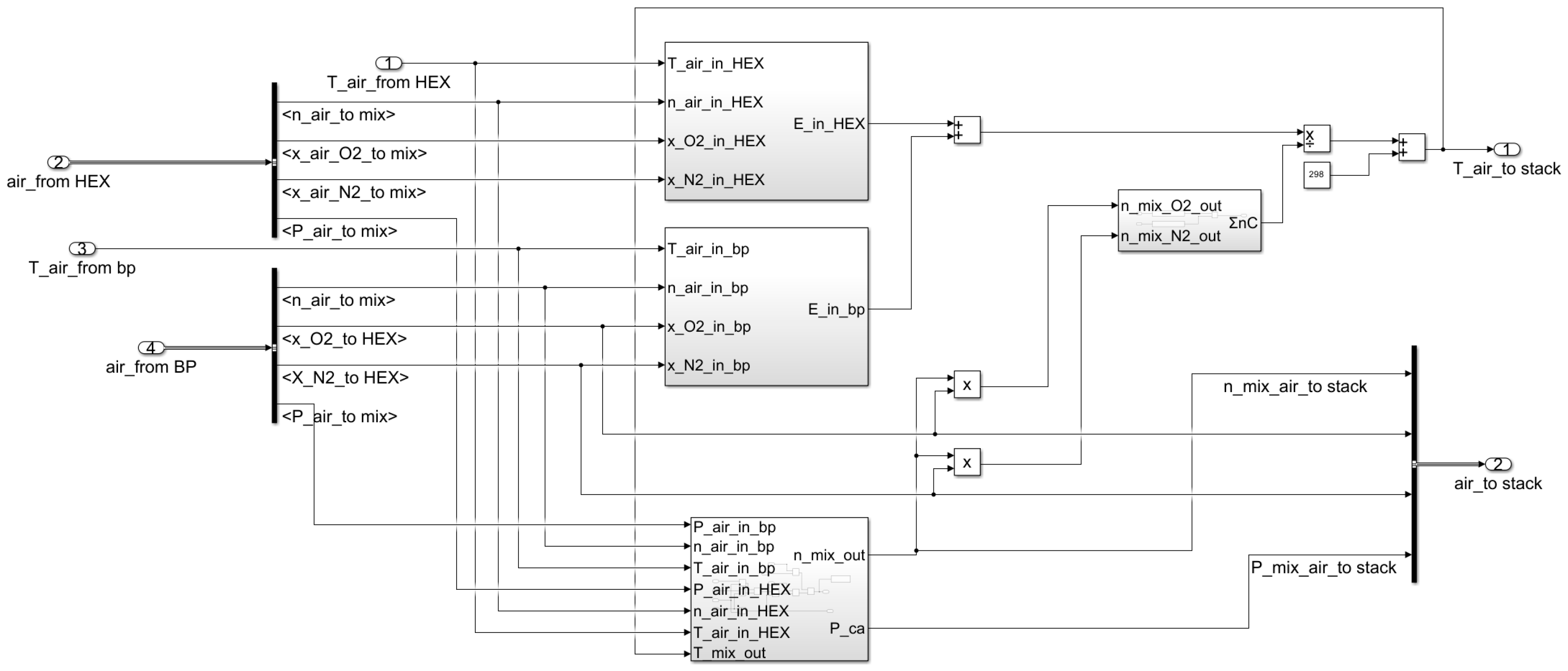
• Mixer model

Figure 6 illustrates the mixer model, which uniformly blends gas streams from different branches based on mass and energy conservation. After mixing, the total mass flow rate can be expressed as

$${\dot{m}}_{mix}=\sum _{i=1}^n{\dot{m}}_i$$

(14)

Figure 6. Mixer Model.

The outlet temperature is calculated based on energy balance:

$$T_{mix}={\displaystyle \frac{{\sum }_{i=1}^n{\dot{m}}_i{c}_{p,i}{T}_i}{{\dot{m}}_{mix}{c}_{p,i}}}$$

(15)

Here, ${\dot{m}}_i$ and $T_i$ represent the mass flow rate and temperature of the $i$-th branch, respectively, while $c_{p,i}$ denotes the specific heat capacity at constant pressure ($\mathrm{J}·{\mathrm{k}\mathrm{g}}^{-1}·{\mathrm{K}}^{-1}$).

2.

Pre-reformer model

Figure 7 illustrates the pre-reformer model, which partially converts hydrocarbon fuels into hydrogen-rich gas prior to entering the SOFC. Its dynamic process can typically be described using a first-order dynamic model:

$${\displaystyle \frac{d{C}_{H_2}}{dt}}={\displaystyle \frac{1}{{\tau }_f}}\left(C_{H_{2,eq}}-C_{H_2}\right)$$

(16)

Figure 7. Pre-reformer Model.

Here, $C_{H_2}$ represents the instantaneous concentration of hydrogen gas ($\mathrm{m}\mathrm{o}\mathrm{l}·{\mathrm{m}}^{-3}$), $C_{H_2,eq}$ denotes the equilibrium concentration ($\mathrm{m}\mathrm{o}\mathrm{l}·{\mathrm{m}}^{-3}$), and ${\tau }_f$ is the reforming time constant (s). For steady-state conditions, this can be further simplified to:

$$C_{H_{2,out}}={\eta }_{ref}·C_{fuel,in}$$

(17)

In this equation, ${\eta }_{ref}$ represents the reforming efficiency of the pre-reformer.

3.

Bypass valve model

The air bypass valve regulates the air flow entering the SOFC or combustion chamber, enabling rapid system load response and temperature control. Its flow characteristics are typically described by the valve opening $u_v$ and the pressure difference $\Delta p$:

$${\dot{m}}_{air}=C_v{u}_v\sqrt{\Delta p \rho }$$

(18)

Here, ${\dot{m}}_{air}$ represents the air flow rate at the valve outlet, $C_v$ denotes the valve flow coefficient, $\rho$ is the fluid density, and $\Delta p=p_{up}-p_{down}$ indicates the pressure difference across the valve (Pa).

The dynamic response of the bypass valve can be simplified to a first-order inertial model:

$${\tau }_v{\displaystyle \frac{d{\dot{m}}_{air}}{dt}}+{\dot{m}}_{air}={\dot{m}}_{air,set}$$

(19)

Here, ${\tau }_v$ represents the valve response time constant, and ${\dot{m}}_{air,set}$ denotes the desired air flow rate. This model reflects the bypass valve’s air regulation and precision, ensuring rapid load adjustment for the system.

4.

Catalytic combustion chamber model

Figure 8 shows the combustion chamber model. The chemical reactions occurring in the catalytic combustion chamber include:

$$2H_2+O_2\to 2H_{2}O$$

(20)

$$2CO+O_2\to 2C{O}_2$$

(21)

Figure 8. Combustion Chamber Model.

For modeling convenience, the combustion chamber is assumed to operate under complete combustion conditions with sufficient oxygen supply, uniform outlet gas properties, and constant thermophysical properties.

Its energy conservation can be expressed as

$${\dot{Q}}_{comb}={\eta }_{cat}·{\dot{m}}_{fuel}·LHV$$

(22)

Among these, ${\dot{Q}}_{comb}$ represents the heat power released during combustion ($\mathrm{J}·{\mathrm{s}}^{-1}$), ${\dot{m}}_{fuel}$ is the fuel mass flow rate ($\mathrm{k}\mathrm{g}·{\mathrm{s}}^{-1}$), LHV indicates the lower heating value ($\mathrm{J}·{\mathrm{k}\mathrm{g}}^{-1}$), and ${\eta }_{cat}$ signifies the catalytic combustion efficiency.

The outlet gas temperature can be calculated using an energy balance equation:

$$T_{out}={\displaystyle \frac{{\dot{Q}}_{comb}+\sum _i{\dot{m}}_i{c}_{p,i}{T}_i}{{\sum }_i{\dot{m}}_i{c}_{p,i}}}$$

(23)

In this model, the summation term $i$ represents the total mass flow entering the combustion chamber and ultimately becoming exhaust gas, while $c_{p,i}$ denotes the corresponding specific heat at constant pressure.

5.

Heat exchanger model

In the SOFC/GT hybrid system, the heat exchanger recovers waste heat from the SOFC exhaust to preheat the fuel and inlet air. The heat transfer power is expressed as

$$Q=UA\Delta T_{lm}$$

(24)

where $Q$ is the heat power transferred by the heat exchanger (W), $U$ is the overall heat transfer coefficient, $A$ is the heat transfer area (${\mathrm{m}}^2$), and $\Delta T_{lm}$ signifies the logarithmic mean temperature difference (K).

The law of conservation of energy is expressed as

$$Q=\dot{m}{c}_p\left(T_{out}-T_{in}\right)$$

(25)

where $Q$ is positive when heat is added to the fluid.

The outlet temperature of the heat exchanger can be calculated based on the law of conservation of energy as

$$T_{out}=T_{in}+{\displaystyle \frac{Q}{\dot{m}{c}_p}}$$

(26)

Here, $\dot{m}$ represents the fluid mass flow rate (kg$·{\mathrm{s}}^{-1}$), $c_p$ denotes the specific heat capacity, and $T_{in}$ and $T_{out}$ are the inlet and outlet temperatures of the fluid, respectively (K).

3.2. GT Subsystem Model

The gas turbine (GT) primarily consists of four components: the compressor model, turbine model, generator model, and shaft model. Its function is to convert the high-temperature energy from the SOFC exhaust into mechanical efficiency, thereby further enhancing the overall energy efficiency of the system.

During modeling, it is assumed that both air and fuel gas behave as ideal gases, all components operate in steady-state conditions, and the compressor and turbine efficiencies are constant values.

The compressor power is given by

$$P_c={\displaystyle \frac{{\dot{m}}_a{c}_p{T}_1}{{\eta }_c}}\left[{\left({\displaystyle \frac{p_2}{p_1}}\right)}^{{\displaystyle \frac{\gamma -1}{\gamma }}}-1\right]$$

(27)

The gas turbine output power is given by

$$P_t={\dot{m}}_g{c}_p{T}_3{\eta }_t\left[1-{\left({\displaystyle \frac{p_4}{p_3}}\right)}^{{\displaystyle \frac{\gamma -1}{\gamma }}}\right]$$

(28)

The net power output of the gas turbine is expressed as

$$P_{GT}=P_t-P_c$$

(29)

The system exhaust temperature is given by

$$T_{out}=T_4-{\displaystyle \frac{P_c}{{\dot{m}}_g{c}_p}}$$

(30)

Among these, ${\dot{m}}_a$ and ${\dot{m}}_g$ represent the air and fuel gas flow rates, $c_p$ denotes the specific heat capacity at constant pressure ($\mathrm{J}·{\mathrm{k}\mathrm{g}}^{-1}·{\mathrm{K}}^{-1}$), $T_1$ is the compressor inlet temperature (K), $\gamma$ is the specific heat ratio, and ${\eta }_c$ and ${\eta }_t$ are the compressor and turbine efficiencies, respectively.

• Compressor model

The compressor supplies pressurized air to the SOFC/GT system. The relationship between the outlet and inlet pressures is given by

$$p_{out}=p_{in}·{\pi }_c$$

(31)

$${\pi }_c={\left(1+{\displaystyle \frac{{\eta }_c{P}_{mech}}{{\dot{m}}_{air}{c}_p{T}_{in}}}\right)}^{{\displaystyle \frac{\gamma }{\gamma -1}}}$$

(32)

Among these, $p_{in}$ and $p_{out}$ represent the compressor inlet and outlet pressures (Pa), respectively; ${\pi }_c$ denotes the compressor pressure ratio; ${\eta }_c$ indicates the isentropic efficiency; $P_{mech}$ signifies the mechanical power driving the compressor (W); ${\dot{m}}_{air}$ denotes the air mass flow rate; $c_p$ and $\gamma$ represent the specific heat at constant pressure and the specific heat ratio, respectively; and $T_{in}$ denotes the compressor inlet temperature.

The air outlet temperature can be calculated using the isentropic relationship as

$$T_{out}=T_{in}\left[1+{\displaystyle \frac{1}{{\eta }_c}}\left({\pi }_c^{{\displaystyle \frac{\gamma -1}{\gamma }}}-1\right)\right]$$

(33)

2.

Turbine model

The turbine model is based on the isentropic expansion relationship:

$$T_{out,is}=T_{in}·{\pi }_t^{{\displaystyle \frac{\gamma -1}{\gamma }}}$$

(34)

Irreversible losses occur during the actual expansion process, so the entropy efficiency of the permeation process is defined as

$${\eta }_t={\displaystyle \frac{T_{in}-T_{out}}{T_{in}-T_{out,is}}}$$

(35)

After processing, the turbine’s actual outlet temperature is obtained as

$$T_{out}=T_{in}-{\eta }_t\left(T_{in}-T_{in}{\pi }_t^{{\displaystyle \frac{\gamma -1}{\gamma }}}\right)$$

(36)

where $T_{in}$ and $T_{out}$ denote the turbine inlet/outlet temperatures, ${\pi }_t={\displaystyle \frac{p_{out}}{p_{in}}}$ represents the pressure ratio, and ${\eta }_t$ is the isentropic efficiency.

The mechanical work produced by expansion is calculated from the conservation of energy as

$$P_t={\dot{m}}_{gas}{c}_p\left(T_{in}-T_{out}\right)$$

(37)

Here, $P_t$ denotes the mechanical power output of the turbine (W), ${\dot{m}}_{gas}$ represents the mass flow rate of gas entering the turbine, and $c_p$ is the specific heat capacity.

For systems coupled with compressors, power balance must also be satisfied:

$$P_t=P_c+P_{load}+P_{loss}$$

(38)

Among these, $P_c$ represents the power consumed by the drive compressor (W), $P_{load}$ denotes the net power supplied to the generator (W), and $P_{loss}$ indicates shaft train losses (W), which can be neglected.

3.3. Validation of SOFC/GT System Simulation Model

To validate the reliability and accuracy of the dynamic model established for the SOFC/GT hybrid system, this study compares simulation results with experimental data from Siemens Westinghouse Power Corporation (SWPC) [42] under steady-state operating conditions. The experimental data are presented in tabular form, with each row corresponding to a specific operating condition and each column corresponding to a measurement or calculation parameter, including current density, SOFC single-cell voltage, pressure ratio, air mass flow rate, turbine inlet temperature, SOFC direct current power, gas turbine alternating current power, system net alternating current power, and system efficiency. All values are steady-state experimental measurements. Some of these parameters were selected for model input and validation in this study. Table 3 presents the comparison between the simulation results obtained in this study and the corresponding experimental measurements from the SWPC. Simulation results demonstrate that the performance metrics obtained using the dynamic model established in this study exhibit excellent consistency with experimental results from the SWPC. This indicates that the constructed model can effectively reflect the steady-state operating characteristics of the SOFC/GT hybrid system, thereby validating the model’s effectiveness and feasibility.

Table 3. Performance Comparison of Hybrid Systems under Rated Conditions.

Parameter	SWPC	SOFC/GT Dynamic Model	Unit
Fuel utilization rate	0.85	0.784202	/
SOFC Single-Cell Operating Voltage	0.610	0.702	V
Pressure ratio	2.9	2.9	/
SOFC Output Power	187	176	kW
System Net Output Power	220	215	kW
GT Rated Speed	70,000	70,000	rpm
GT Output Power	47	39.98	kW
Turbomachinery Efficiency	94	94	%

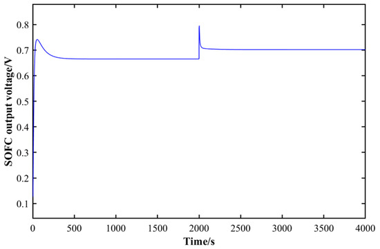
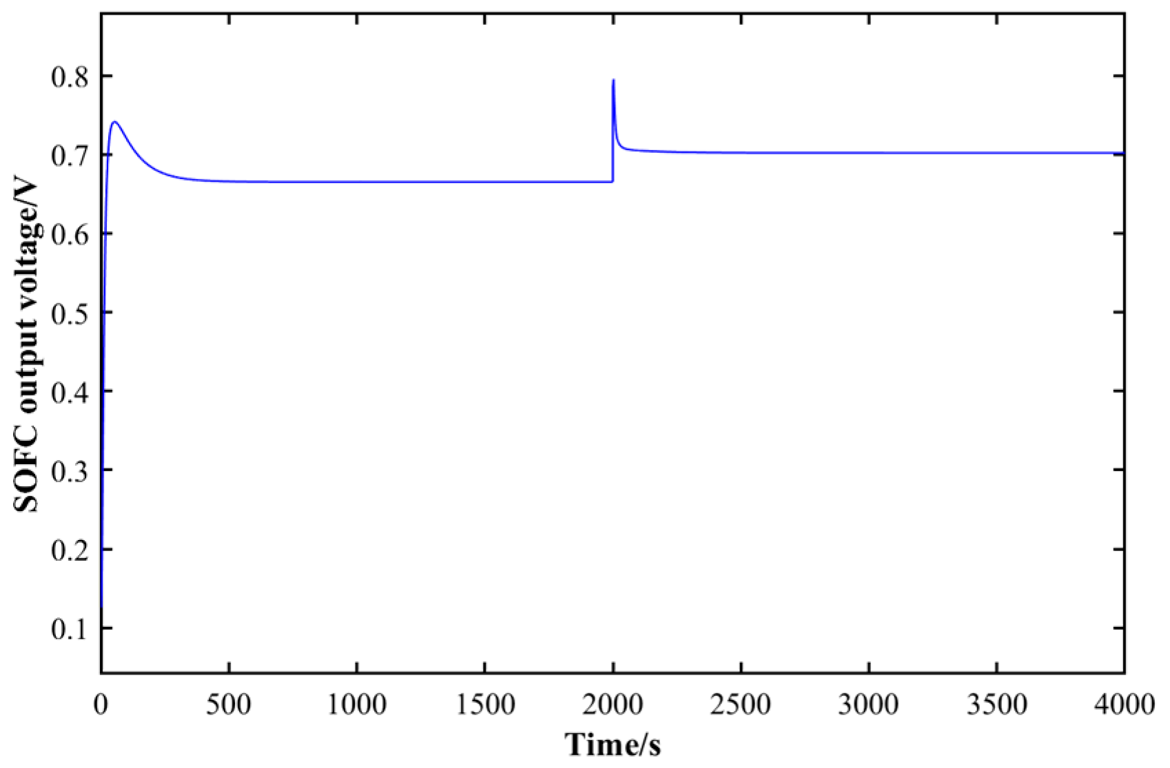
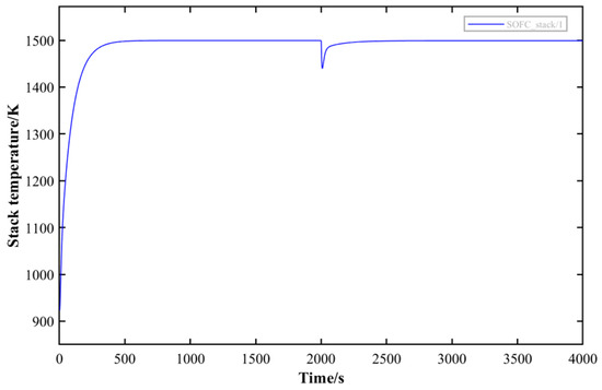
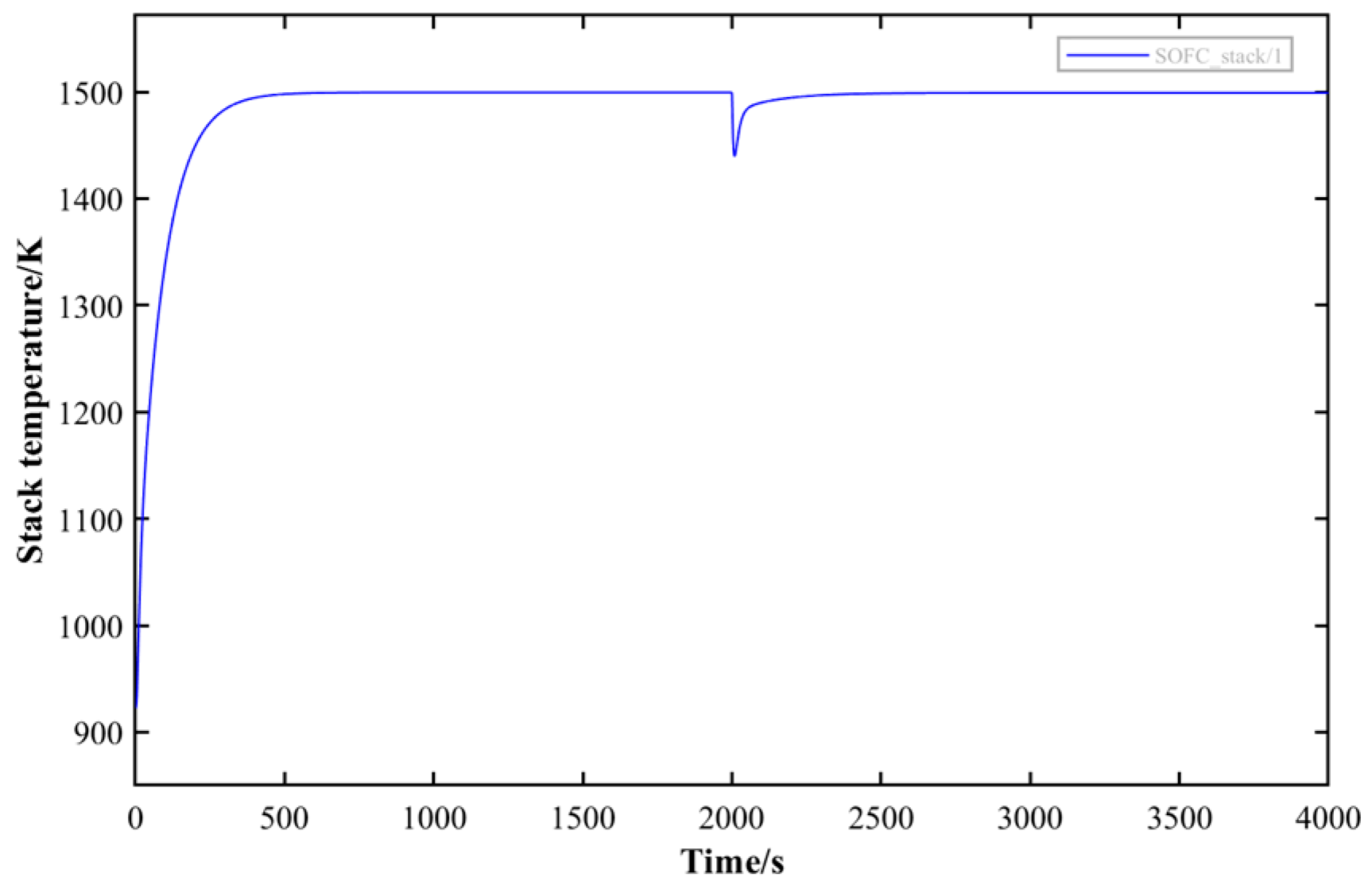
In the next analysis, the impact of fuel utilization efficiency on system performance was investigated. Figure 9 and Figure 10 show the SOFC output voltage and SOFC operating temperature as fuel utilization increases. Improved fuel utilization alters the equilibrium between exothermic reactions within the fuel cell and the cooling effect of gas flow, thereby inducing temperature changes.

Figure 9. SOFC Output Voltage with Increased Fuel Utilization.

Figure 10. SOFC Operating Temperature with Increased Fuel Utilization.

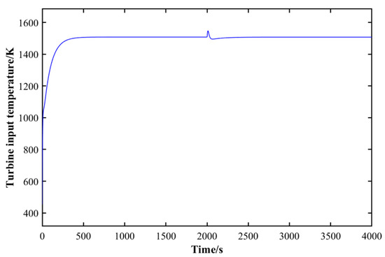
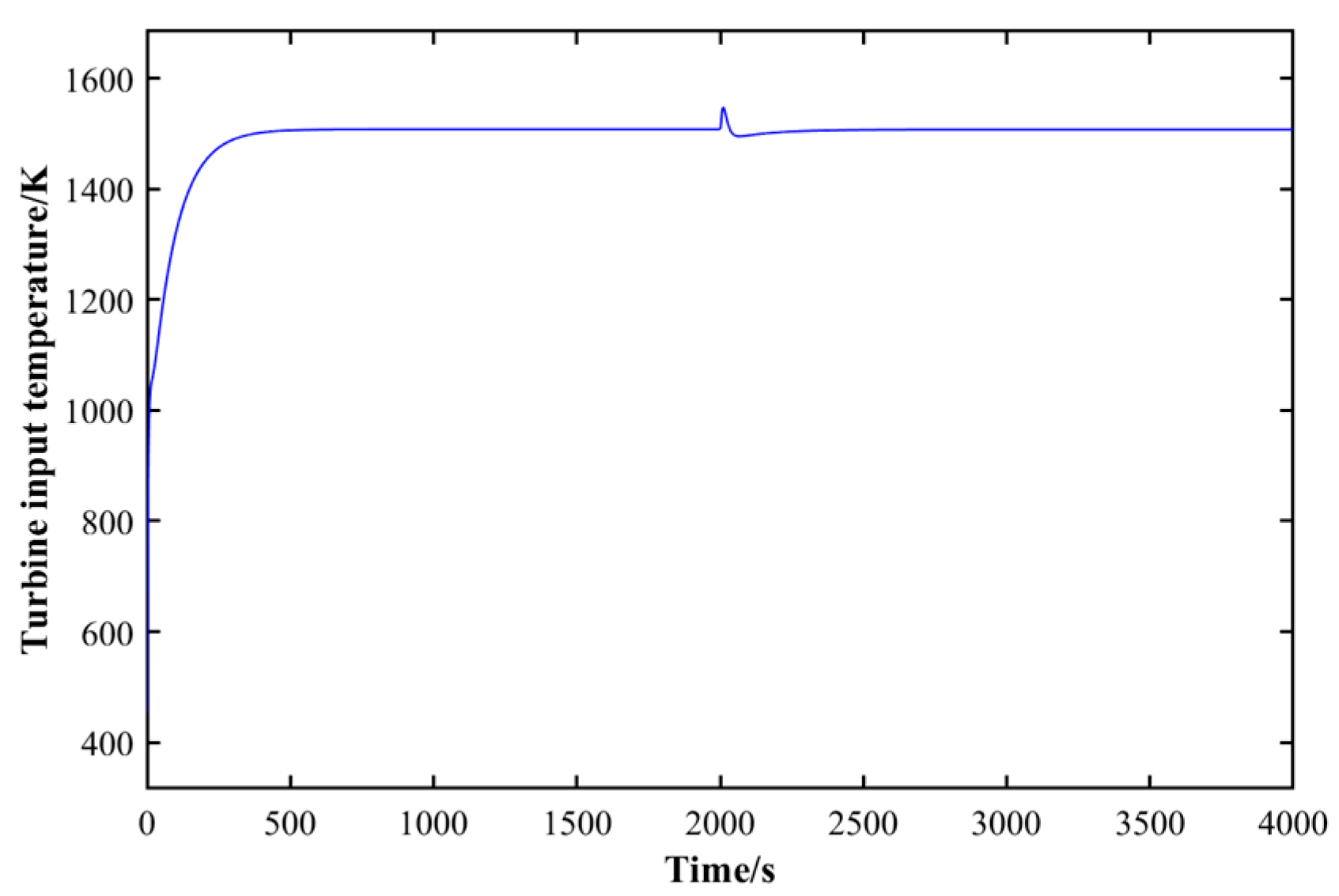
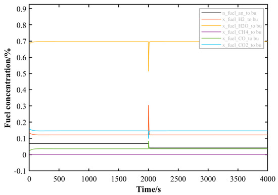
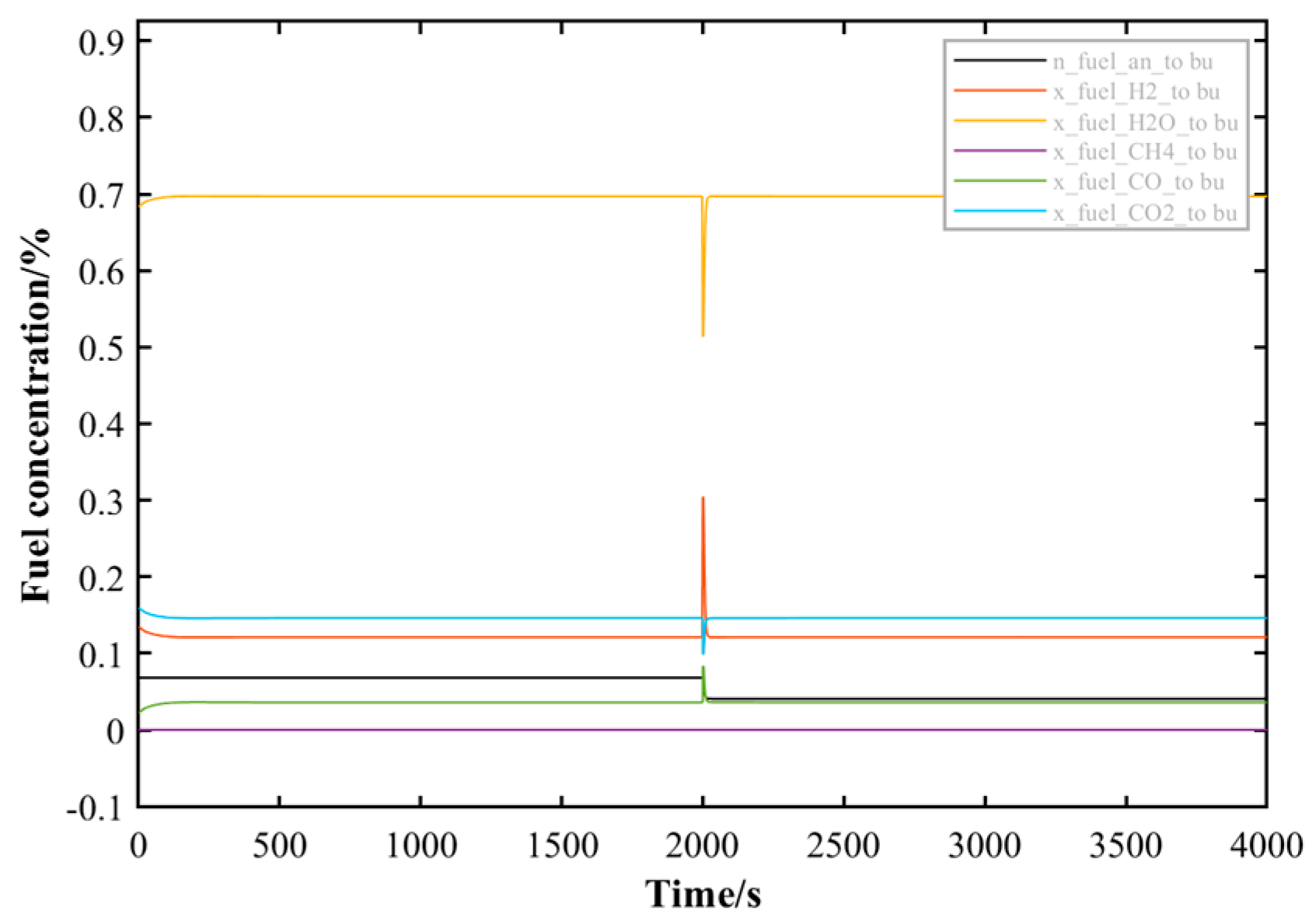
Figure 11 and Figure 12 show the turbine inlet temperature characteristics and combustible concentration performance, respectively, as fuel utilization increases. Changes in fuel utilization alter the exhaust temperature and composition of the SOFC, thereby affecting the turbine inlet temperature (TIT) at the combustion chamber outlet. x_fu-el_H2_to_bu and x_fuel_CO_to_bu represent the combustible hydrogen and carbon monoxide remaining in the anode off-gas, respectively. x_fuel_H2O_to_bu and x_fuel_CO2_to_bu represent the non-combustible water vapor and carbon dioxide, respectively. As fuel utilization increases, more hydrogen is consumed within the fuel cell stack, leading to a significant reduction in combustible components—particularly hydrogen concentration—within the anode exhaust gas.

Figure 11. Turbine input temperature when fuel utilization increases.

Figure 12. Fuel concentration when fuel utilization increases.

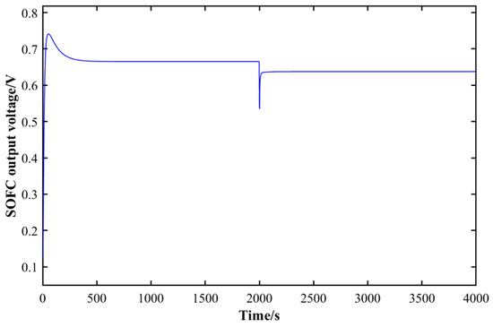
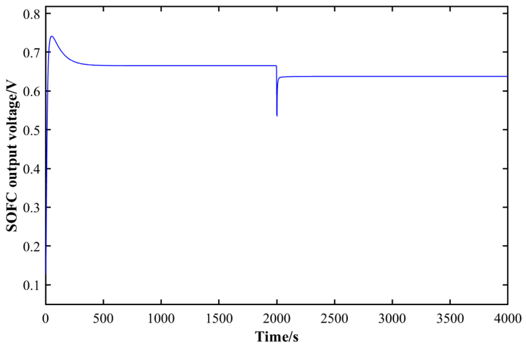
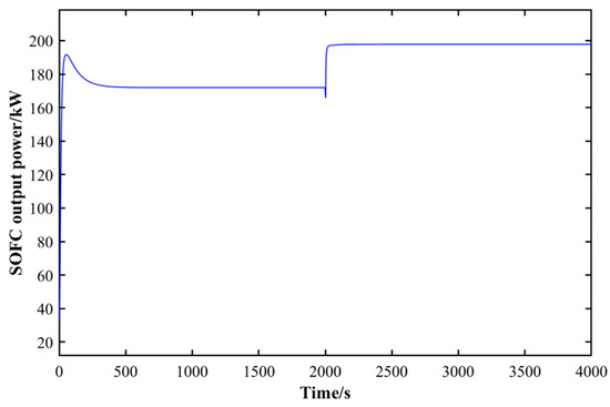
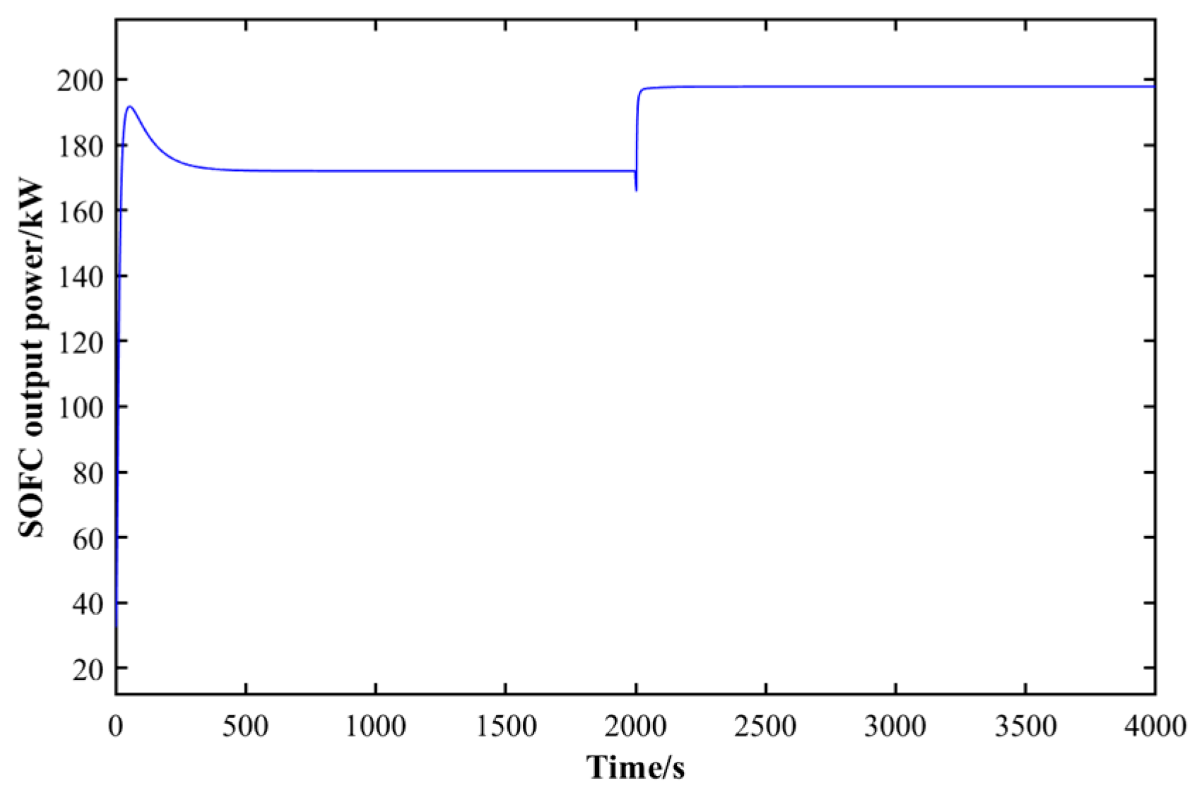
Figure 13 and Figure 14 show the dynamic response of the SOFC output voltage and output power when the current step increases by 20%. Sudden increases in current can intensify various polarization effects within the battery, causing the SOFC output voltage to decrease by approximately 7.53%. Despite the voltage drop, the current increased to a greater extent, resulting in an overall rise in the stack’s output power. From the perspective of time response characteristics, both the output voltage and power exhibit a gradual decay process. The initial changes are relatively pronounced, which are followed by a gradual reduction in fluctuation amplitude, ultimately reaching a stable state.

Figure 13. SOFC output voltage when the current step increases by 20%.

Figure 14. SOFC output power when the current step increases by 20%.

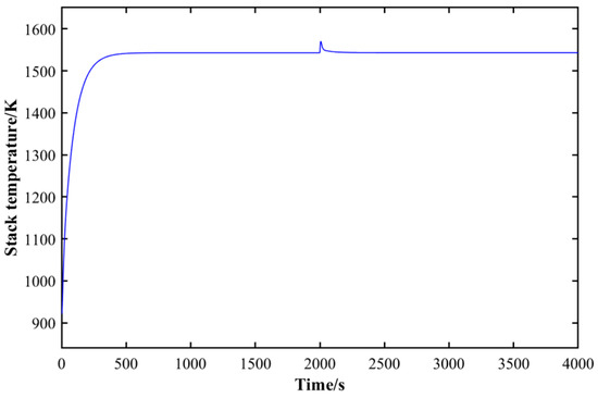
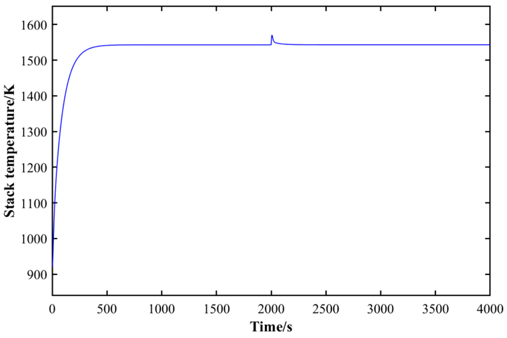
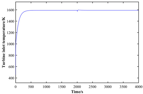
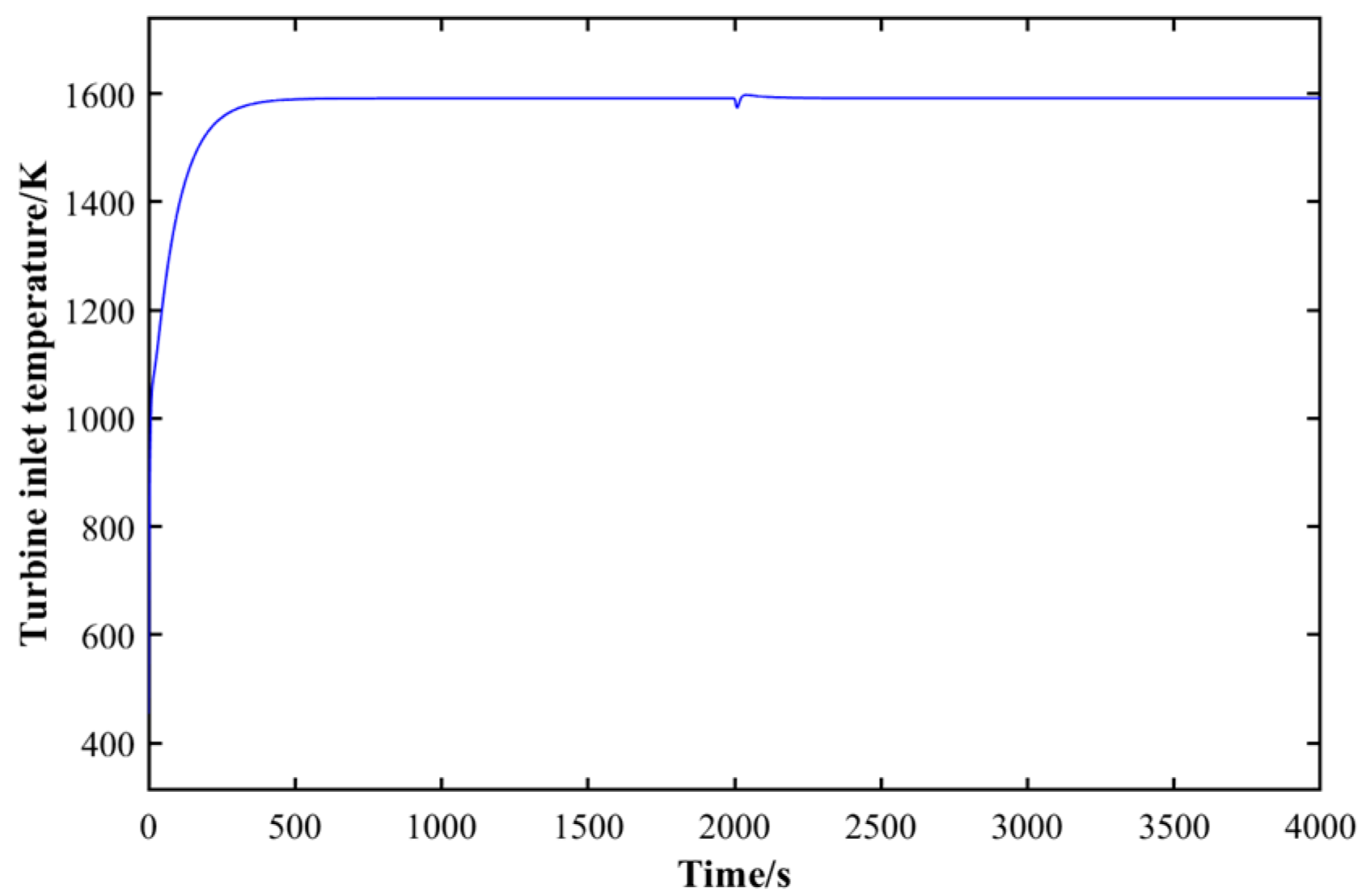
Figure 15 and Figure 16 show the dynamic response curves for the SOFC operating temperature and turbine inlet temperature, respectively. As the current increases, the electrochemical reaction rate intensifies, leading to a rise in the reaction heat release. An increase in current indicates a reduction in combustible gases within the anode exhaust, leading to a decrease in residual fuel entering the combustion chamber. This results in a drop in gas temperature at the combustion chamber outlet, consequently lowering the TIT. This dynamic response characteristic reflects the thermal-energy coupling mechanism between the SOFC and GT.

Figure 15. SOFC operating temperature when the current step increases by 20%.

Figure 16. Turbine inlet temperature when the current step increases by 20%.

4. Case Study

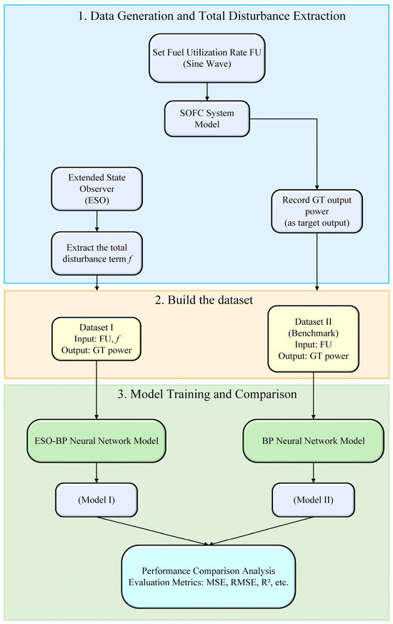
This section outlines the overall workflow employed in the experiment, covering data generation, perturbation extraction, dataset construction, model training, and performance comparison. Figure 17 illustrates the overall process of this study. First, by setting the fuel utilization rate to vary over time, the SOFC/GT hybrid system model was simulated to obtain the system’s input and output data. Simultaneously, the total disturbance to the system is estimated using an extended state observer, thereby obtaining the disturbance term $f$. Based on this, two datasets were constructed: Dataset I, with fuel utilization rate and total disturbance as inputs and GT power output as the output, was used to train an ESO-based BP neural network. Dataset II, using only FU as input, served as the baseline dataset for training a traditional BP neural network. Subsequently, both models were trained and tested under identical conditions. Their predictive performance was compared using RMSE, MSE and ${\mathrm{R}}^2$ metrics to evaluate the improvement in power forecasting accuracy achieved by incorporating ESO disturbance information.

Figure 17. Method Flowchart.

4.1. Construction of the GT Power Forecasting Dataset

To validate the improvement in neural network prediction performance achieved by the total disturbance term estimated by the extended state observer, a GT power prediction dataset was constructed based on simulation results from the SOFC/GT system. The dataset is used to train and validate the subsequently proposed ESO-BP neural network model.

By adjusting key operating parameters, such as the fuel utilization rate, the corresponding GT output power and total disturbance estimated by the ESO were obtained for the system. Therefore, the entire dataset comprises three variables: fuel utilization rate, total disturbance, and gas turbine output power. To analyze the impact of introducing ESO disturbance terms on prediction accuracy, two datasets were designed for comparison in this study. The first dataset uses fuel utilization rate (FU) and total disturbance $f$ as inputs, with GT power as the output, for training the ESO-BP neural network model. The second dataset uses only FU as input, with GT power as the output, for training the traditional BP neural network model. The two datasets are consistent in terms of sample size, distribution range, and preprocessing methods, differing only in the input feature dimensions.

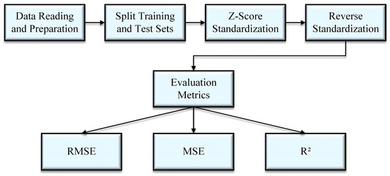
This study extracted operational data from the SOFC/GT system simulation model, collected at a fixed sampling interval of $\Delta t=1 \mathrm{s}$, yielding a total of 4000 discrete data points. This sampling frequency can fully capture the dynamic changes in variables such as gas turbine power and fuel utilization rate while ensuring the simulation time and data processing capacity. Through observation of the data training process, the training error of the BP neural network stabilizes when the sample size reaches approximately 4000, with a noticeable improvement in generalization performance. Further expanding the dataset yields limited gains in accuracy. Therefore, 4000 samples were selected as the dataset size to strike a balance between computational cost and model performance. The collected data is randomly split into training and test sets in an 8:2 ratio. To eliminate dimensional differences and accelerate network convergence, both inputs and outputs are sampled and normalized using z-scores as follows:

$$x_{std}={\displaystyle \frac{x-\mu }{\sigma }}$$

(39)

Here, $\mu$ and $\sigma$ represent the sample mean and standard deviation, respectively. The normalized data is used for neural network training. After training, the original physical quantities are restored through denormalization, ensuring the interpretation and physical significance of the prediction results. Figure 18 shows the data preprocessing and model evaluation flowchart.

Figure 18. Data Preprocessing and Model Evaluation Flowchart.

Table 4 presents the composition of the dataset. Dataset I includes two inputs, FU and the total disturbance term $f$, and was used to analyze the impact of $f$ on gas turbine power prediction performance. Dataset II contains only FU as the input variable and was used to compare whether incorporating $f$ improves the model’s prediction accuracy.

Table 4. Data Set Composition Table.

Dataset ID	Input Variables	Output Variable	Purpose
Dataset I	Fuel Utilization Factor FU, Total Disturbance Term $f$	Gas turbine power	Compare with Dataset II to see if $f$ improves the effect.
Dataset II	Fuel Utilization Factor FU	Gas turbine power	Serve as a baseline

4.2. Evaluation Indicators

The core objective of this study is to quantitatively analyze the role of ESO disturbance terms in GT power forecasting by comparing the prediction results of neural networks with and without disturbance terms. Two sets of data were input into BP neural networks with identical structures and parameters for training. The prediction results were compared with actual power values, and performance evaluation was conducted using metrics such as Mean Squared Error (MSE), Root Mean Squared Error (RMSE), and the coefficient of determination (${\mathrm{R}}^2$).

The prediction results are evaluated using MSE, RMSE, and ${\mathrm{R}}^2$, with the mathematical expressions as follows:

$$\mathrm{M}\mathrm{S}\mathrm{E}={\displaystyle \frac{1}{N}}\sum _{i=1}^N{\left(y_i-{\widehat{y}}_i\right)}^2$$

(40)

$$\mathrm{R}\mathrm{M}\mathrm{S}\mathrm{E}=\sqrt{{\displaystyle \frac{1}{N}}\sum _{i=1}^N{(y_i-{\widehat{y}}_i)}^2}$$

(41)

$${\mathrm{R}}^2=1-{\displaystyle \frac{{\sum }_{i=1}^{N=1}\left({\left(y_i-{\widehat{y}}_i\right)}^2\right)}{{\sum }_{i=1}^N{\left(y_i-\overline{y}\right)}^2}}$$

(42)

Here, $y_i$ represents the actual power, ${\widehat{y}}_i$ denotes the predicted power, $\overline{y}$ is the mean of the actual power, and $N$ is the sample size. Smaller values of MSE and RMSE indicate lower prediction errors, while a coefficient of determination ${\mathrm{R}}^2$ closer to 1 signifies stronger fitting capability.

4.3. Benchmark Strategy

4.3.1. BP Neural Network for Raw Features

The BP neural network is adopted as the primary method, and it is compared with three classical models: decision trees, support vector machines, and random forests. The BP neural network employs the fitnet function to construct a single-hidden-layer structure and utilizes the trainlm algorithm for training, enabling it to capture the nonlinear relationship between features and power. Among the comparison models, the decision tree serves as a basic interpretable reference, the random forest represents ensemble learning methods, and the support vector machine demonstrates the performance of traditional kernel-based approaches.

4.3.2. Decision Tree Model

A decision tree is a supervised learning algorithm that utilizes a tree structure to build predictive models by recursively partitioning the feature space [43]. Its core principle involves selecting optimal features for node splitting to maximize the purity of child nodes. This study employs MATLAB R2023a’s fitrtree function to implement regression decision trees, which are constructed based on the Classification and Regression Trees (CART) framework. Model parameters are set as follows: the splitting criterion employs the principle of minimizing mean squared error and the maximum depth is unrestricted to allow full growth. The advantages of decision trees as a benchmark strategy lie in their simple and intuitive model structure, high computational efficiency, and the ability to directly output feature importance rankings.

4.3.3. Support Vector Machine Model

Support Vector Machines (SVMs) are classical machine learning algorithms based on statistical learning theory and the principle of minimizing structural risk. In linearly inseparable scenarios, they employ kernel techniques to map original features into high-dimensional spaces and seek optimal regression hyperplanes within these spaces [44]. This study employs support vector machines as one of the benchmark strategies, implemented using MATLAB’s fitrsvm function. Support vector machines, as a powerful representative algorithm in traditional machine learning, excel through minimizing structural risk. They achieve strong generalization performance through finding the optimal regression hyperplane.

4.3.4. Random Forest Model

Random Forest is an ensemble learning algorithm proposed by Breiman [45] that enhances model accuracy and robustness by constructing multiple decision trees and combining their prediction results. By constructing multiple decision trees and integrating their prediction results, the model’s accuracy and robustness are enhanced. This algorithm employs bootstrap sampling to generate multiple subsamples from the original training dataset, providing each decision tree with slightly different training data. Simultaneously, it randomly selects feature subsets during node splitting. This dual randomization mechanism effectively reduces model variance and suppresses overfitting. This study employed MATLAB’s TreeBagger function to implement a random forest regression model with 50 trees. The number of trees was selected based on performance convergence observed on the training dataset, where metrics such as RMSE are stabilized. This choice ensures stable and reliable predictions while avoiding overfitting.

4.4. Simulation Results

4.4.1. Training and Testing Performance Evaluation of the BP Neural Network Power Forecasting Model

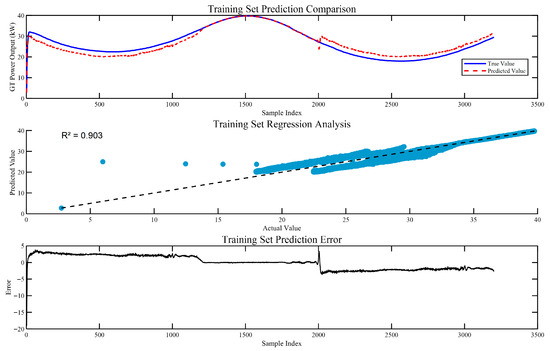
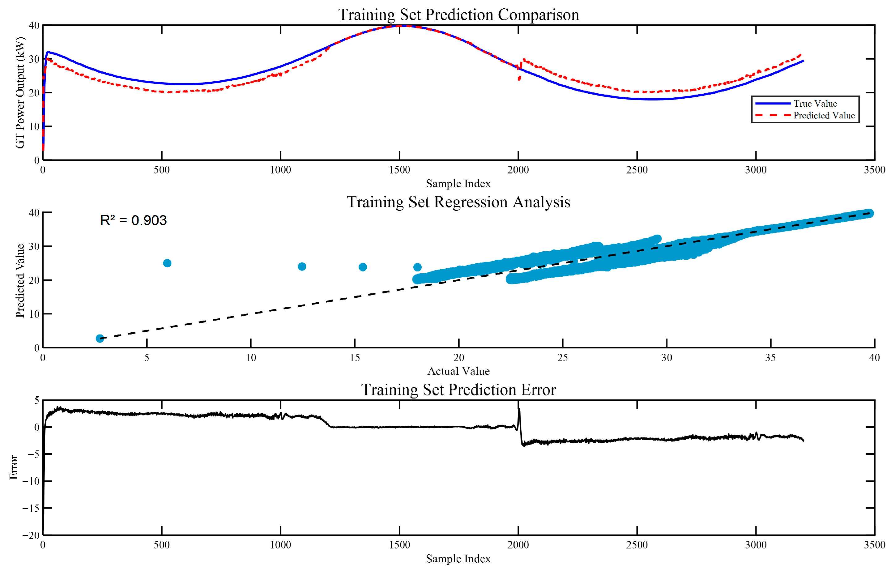
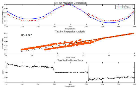
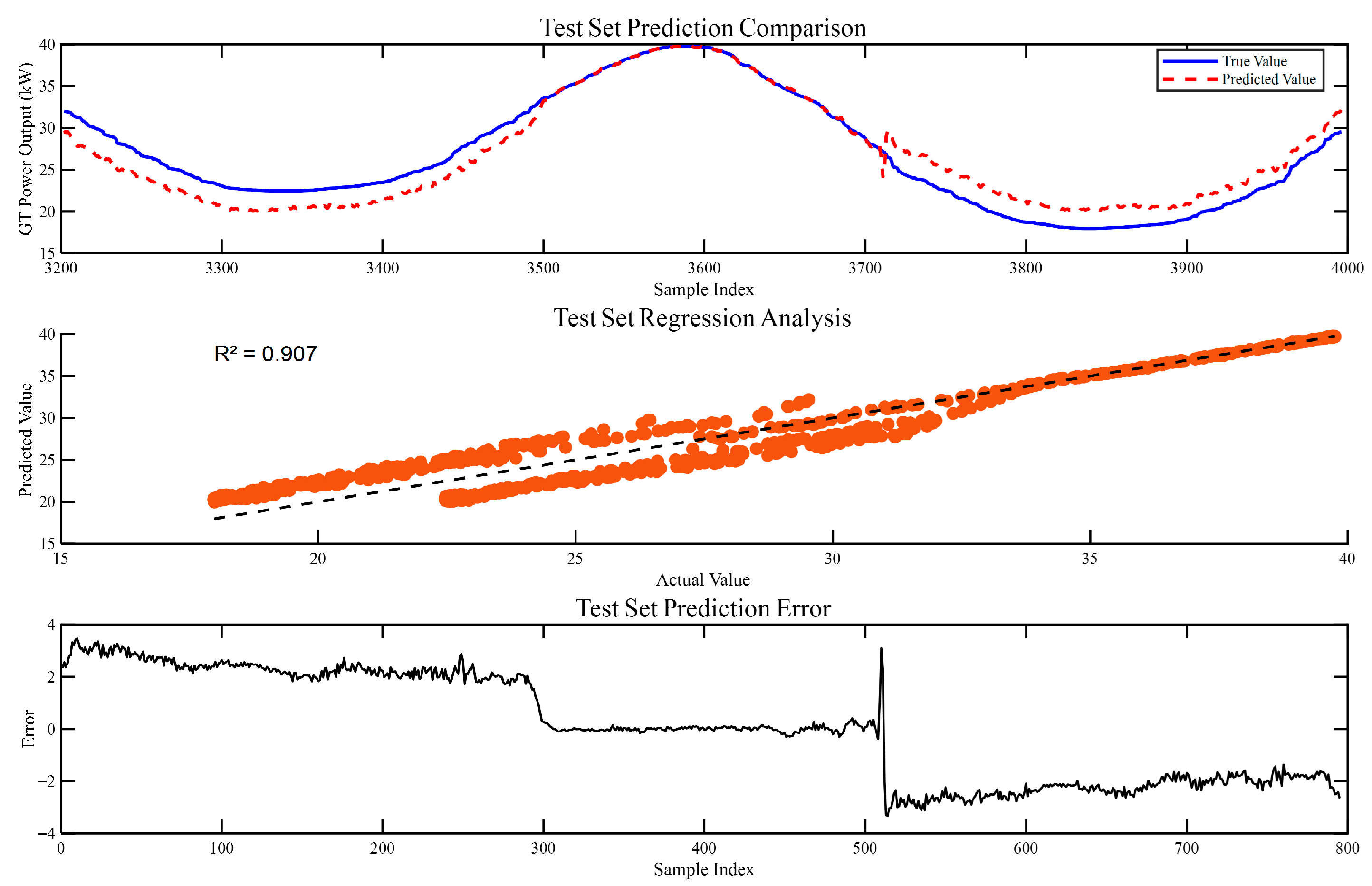
To validate the effectiveness of the BP neural network-based model for predicting gas turbine power, performance evaluations were conducted on both the training and test datasets. During the training phase, the model participates in learning using the training set, and its predictions are compared against the actual outputs. Figure 19 and Figure 20 present the prediction performance evaluation results of the neural network model on the training and test datasets, respectively. As shown in the figures, the predicted power output closely follows the actual values, indicating that the proposed model effectively captures the underlying nonlinear relationship between input features and system power. To further quantitatively evaluate the model performance, key statistical metrics including MSE, RMSE, and R² are analyzed. Table 5 lists their primary evaluation metrics. On the training dataset, the model achieves an MSE of 4.1666 and an RMSE of 2.0412, with an R² value of 0.9026. On the test dataset, the MSE and RMSE are 4.0081 and 2.0020, respectively, while the R² value slightly increases to 0.9075. Compared with the training results, the test MSE and RMSE decrease by approximately 3.8% and 1.9%, respectively, while the R² value improves by about 0.5%. This indicates that the model does not suffer from overfitting and maintains consistent prediction accuracy on unseen data. The close agreement between training and test performance demonstrates the robustness and generalization capability of the proposed neural network model. After completing training set validation, the trained model is applied to the test set to evaluate its predictive capability on unseen data. Test results indicate that the model maintains high predictive accuracy on the test set, with good consistency between predicted values and actual values. This further demonstrates that the constructed BP neural network model possesses strong generalization capabilities, enabling it to predict gas turbine power with high accuracy. This provides a solid foundation for subsequent research.

Figure 19. Evaluation of Neural Network Model Prediction Performance on the Training Set.

Figure 20. Evaluation of Neural Network Model Prediction Performance on the Test Set.

Table 5. Performance Comparison Between Training and Test Sets.

Evaluation Metric	Training Set Performance	Test Set Performance
MSE	4.1666	4.0081
RMSE	2.0412	2.0020
R2	0.9026	0.9075

4.4.2. Ablation Experiment

To further analyze the impact of the total disturbance term $f$ extracted from ESO on the model’s predictive performance, an ablation study was designed. In the simulation, fuel utilization was set as a sinusoidal signal to construct operating condition data with dynamic fluctuation characteristics. Two model sets were developed for comparison: Model A used both fuel utilization and disturbance term $f$ as inputs, while Model B used only fuel utilization as input. The network architecture, training parameters, and data partitioning of the two model sets remain identical, differing only in their input features. By evaluating prediction results on the same test set, we can compare and analyze the contribution of the perturbation term $f$ to prediction performance.

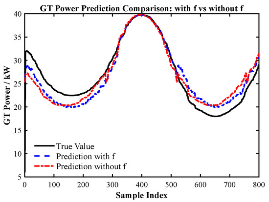
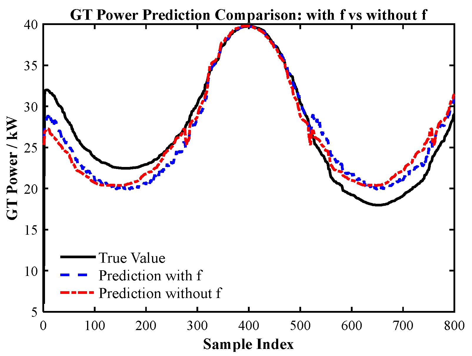
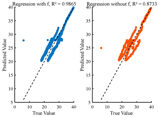
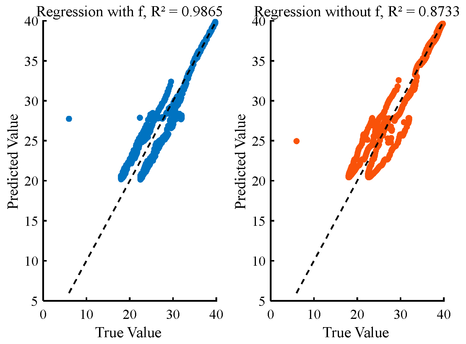
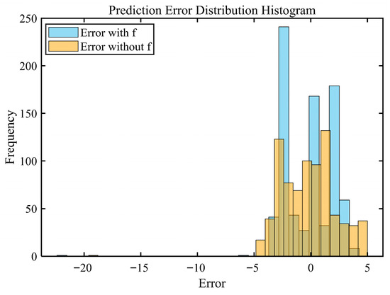
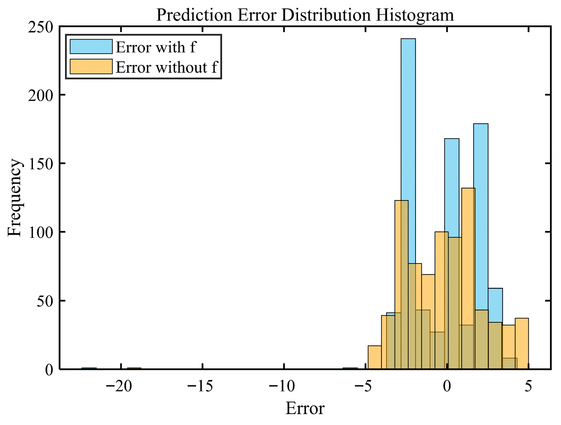
Figure 21 displays the output power prediction results for two sets of data. Figure 22 presents a comparison of the regression performance between the two models. Model A, which incorporates a disturbance term, achieves a coefficient of determination ${\mathrm{R}}^2$ of 0.9865, surpassing Model B’s 0.8733. This demonstrates that adding the disturbance term enhances the model’s fitting accuracy to the actual output. Figure 23 shows the histogram of error distribution, reflecting the statistical characteristics of the two sets of prediction errors. To more intuitively evaluate the impact of the disturbance term $f$ on prediction performance, the primary performance metrics of the two model sets were calculated separately, as shown in Table 6.

Figure 21. Gas Turbine (GT) Power Comparison.

Figure 22. Regression Comparison.

Figure 23. Prediction Error Distribution Histogram.

Table 6. Performance Metrics of Models with and without $f$.

Evaluation Metric	Model A (with f)	Model B (Without f)
MSE	0.5814	5.4512
RMSE	0.7625	2.3348
R2	0.9865	0.8733

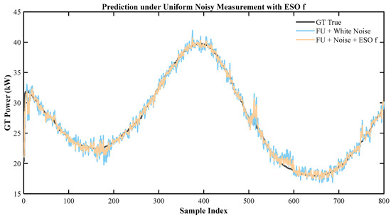
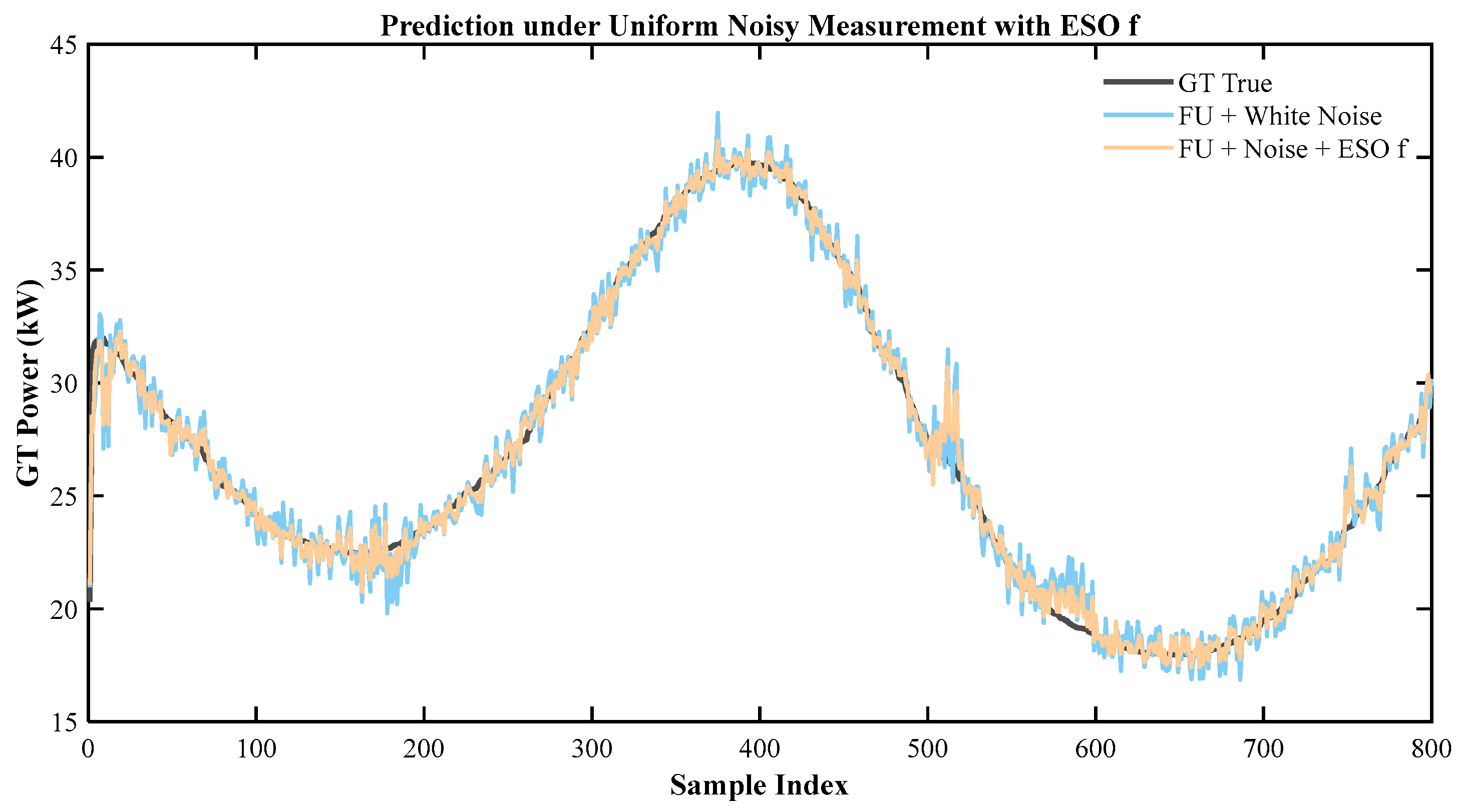
Under low-noise conditions, Figure 24 visually demonstrates signal contrast. This figure presents results from baseline prediction and noise addition, where the effect of adding f-values is clearly visible. For larger noise conditions, the visual difference becomes less noticeable due to the high noise level. Therefore, Table 7 presents quantitative metrics including MSE, RMSE, MAE, and ${\mathrm{R}}^2$. These metrics demonstrate that the proposed method still achieves improved performance compared to the baseline approach. Specifically, the RMSE decreased from 1.434 to 1.286, the MAE decreased from 1.113 to 0.911, and the R² increased from 0.952 to 0.961. These results demonstrate that the proposed method improves performance under low-noise conditions and still provides measurable gains under higher-noise conditions.

Figure 24. Prediction under low measurement noise.

Table 7. Quantitative Performance under Noisy Measurement Conditions.

Evaluation Indicators	FU + Noise	FU + Noise + f	Improvement
MSE	2.0556	1.6531	Reduction ≈ 19.6%
RMSE	1.4338	1.2857	Reduction ≈ 10.3%
MAE	1.1128	0.9108	Reduction ≈ 18.2%
${\mathrm{R}}^2$	0.95188	0.96131	Increase ≈ 0.99%

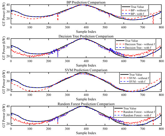
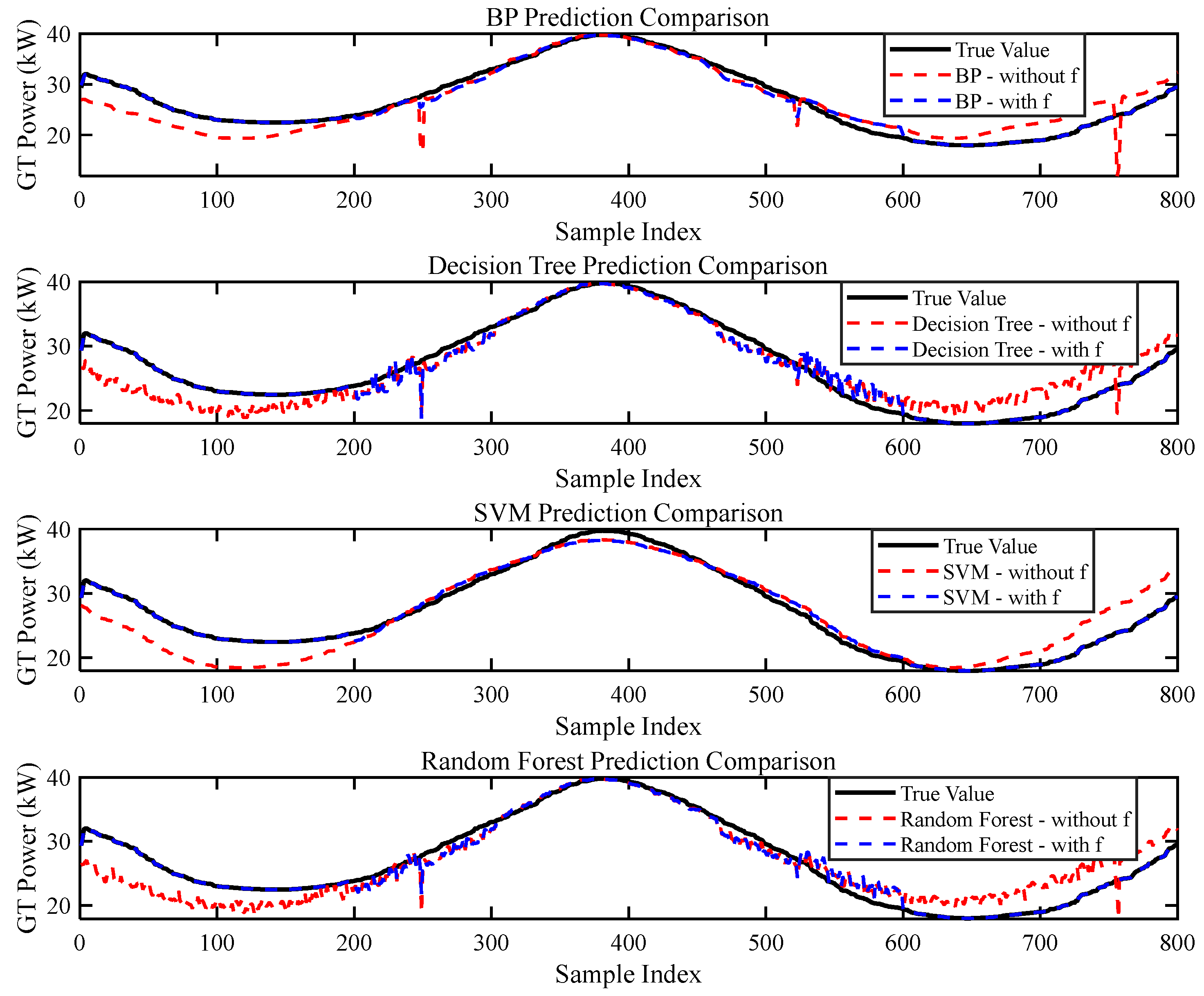
Figure 25 presents the prediction outputs of the BP neural network, decision tree, SVM, and random forest under the single input of FU and the combined input of FU + $f$. It can be observed that all models exhibit certain patterns: after introducing the $f$ estimation value, the fitting degree of the predicted values to the actual power curves significantly improves.

Figure 25. Comparison of Prediction Results Across Different Models with and without the Disturbance Term $f$.

Specifically, after introducing the disturbance term $f$, the BP neural network can more accurately capture power variation trends, significantly reducing the systematic bias that occurs when only FU is used as input in both the valley and peak regions. The FU model for decision trees and random forests exhibits significant fluctuations in areas with data variations, whereas FU + $f$ markedly reduces such volatility, yielding more stable prediction outcomes. The SVM model exhibits significant underfitting in the curve under the FU condition, whereas incorporating $f$ enables better capture of nonlinear trends, achieving high consistency with actual values.

4.4.3. Method Validation

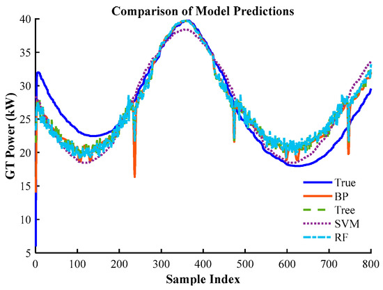
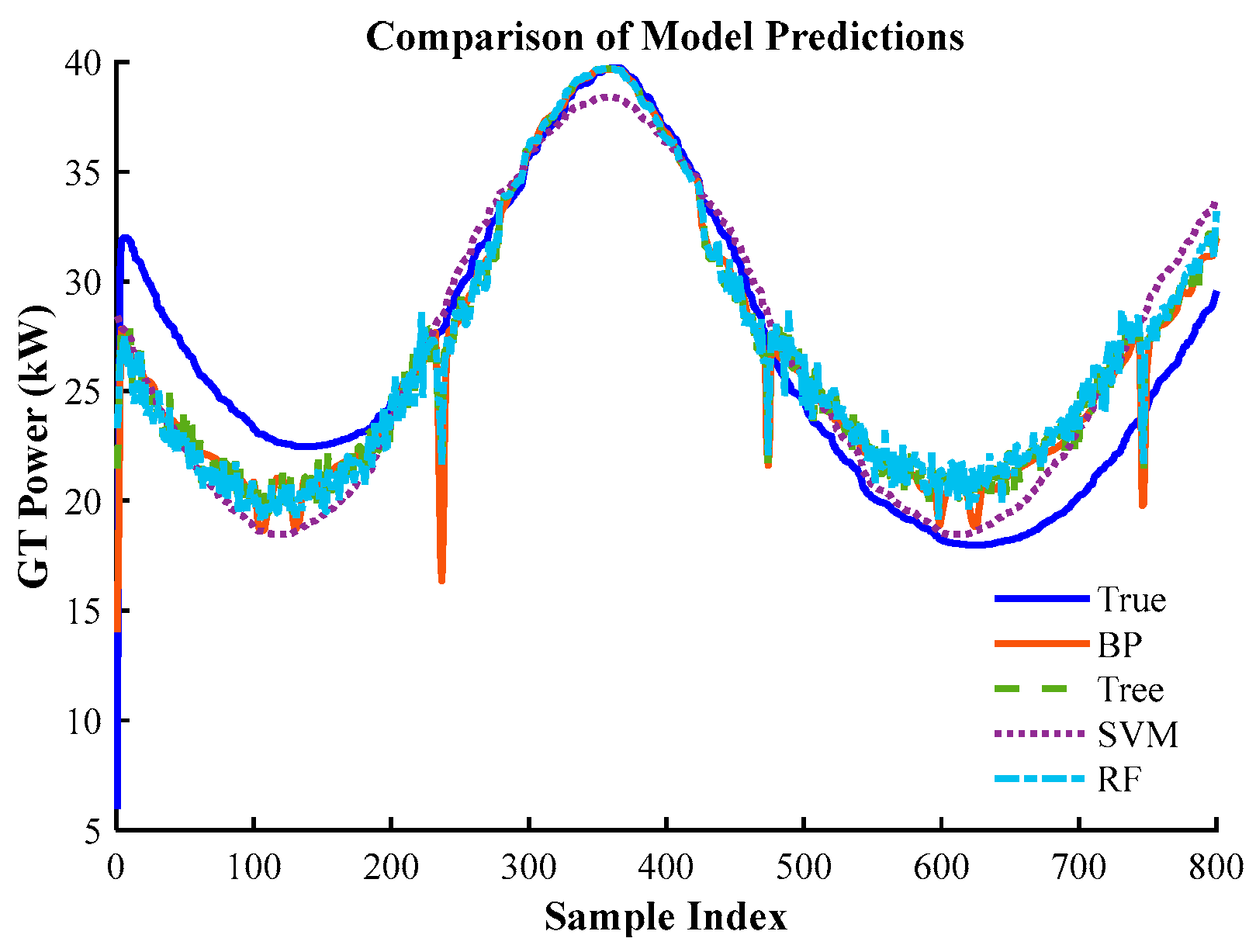
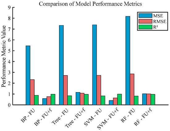
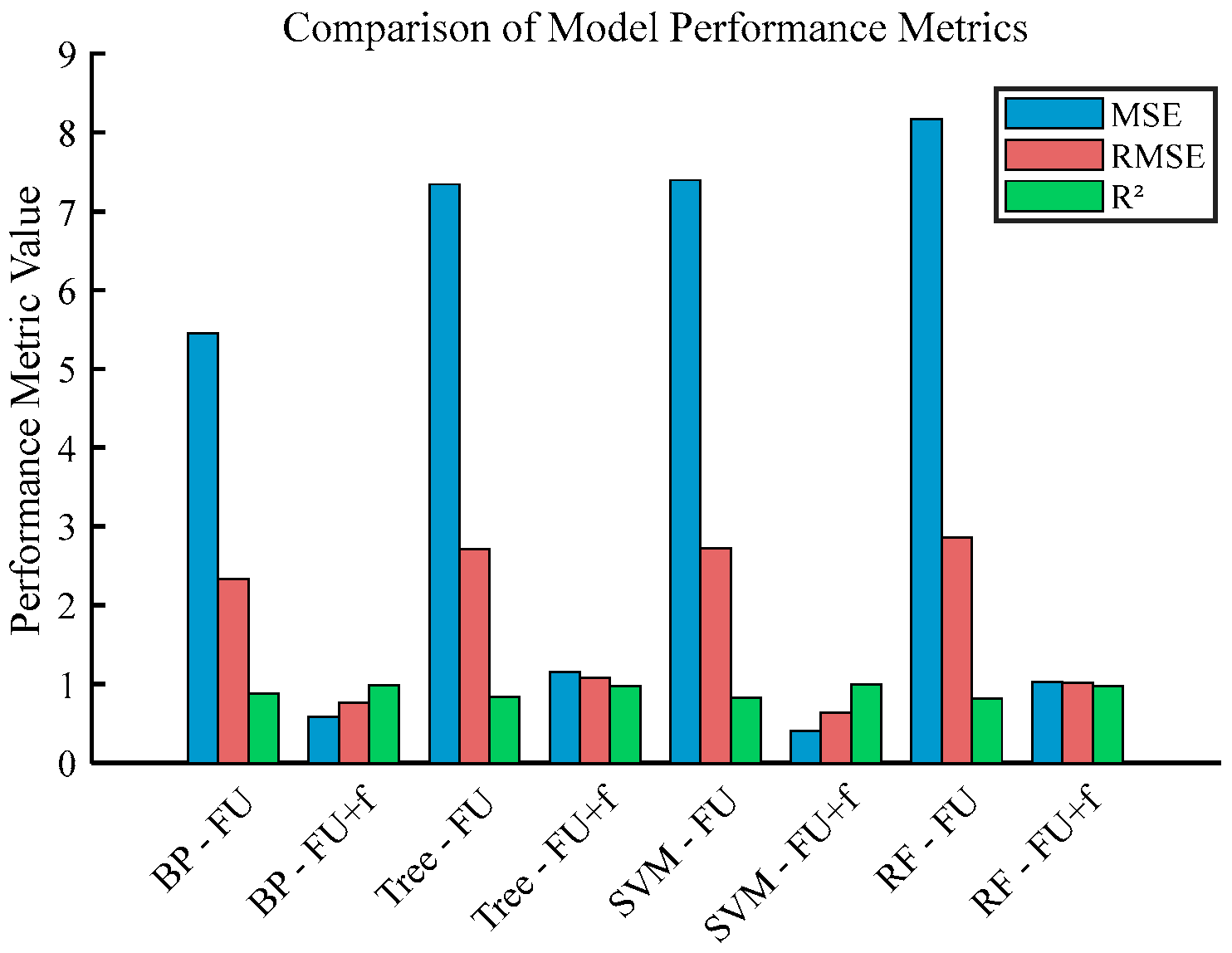
To further validate the improvement in predictive model performance achieved by incorporating the total disturbance estimated by ESO into the input features, we selected three regression models—decision trees, support vector machines, and random forests—for a unified comparison with the BP neural network. This comparison was conducted on the data constructed earlier to assess the impact of the disturbance term $f$ on predictive performance. The results of the operation are shown in Figure 26 and Figure 27. When fuel utilization rate is the sole input, the predictive accuracy of each model is comparable, but their overall performance remains limited. After incorporating the ESO perturbation term, the performance of all models improved significantly, indicating that perturbation information provides additional dynamic characteristics to the models, making it easier for them to capture the patterns of power variation with perturbations. As shown in Table 8, SVM achieved a higher ${\mathrm{R}}^2$ after incorporating $f$, demonstrating optimal performance. Random Forest exhibited the greatest improvement, indicating strong learning capabilities. Although the BP network showed a relatively smaller improvement, its predictive performance still improved significantly, suggesting it possesses a certain degree of responsiveness to disturbance information. From a quantitative perspective, all models achieved significant improvements after incorporating the disturbance term $f$. The MSE and RMSE of the BP neural network decreased by approximately 89.33% and 67.34%, respectively, while ${\mathrm{R}}^2$ improved by 0.1132. The MSE and RMSE of the decision tree decreased by 84.29% and 60.38%, respectively, and ${\mathrm{R}}^2$ increased by 0.1438. Support Vector Machine demonstrated the most outstanding performance, with MSE and RMSE decreasing by 95.55% and 76.67%, respectively, and ${\mathrm{R}}^2$ increasing by 0.1625; Random Forest also saw MSE and RMSE decrease by 87.43% and 64.53%, respectively, with ${\mathrm{R}}^2$ improving by 0.1660. Overall, the introduction of the disturbance term $f$ consistently improves the predictive quality of various regression models, further demonstrating the effectiveness of disturbance information estimated by ESO in power forecasting.

Figure 26. Regression Comparison of Four Models.

Figure 27. Comparison of Model Performance Metrics.

Table 8. Performance Metrics Comparison of Models with and without $f$.

Model	MSE	RMSE	R2
BP-FU	5.4512	2.3348	0.8733
BP-FU + f	0.5814	0.7625	0.9865
Tree-FU	7.3406	2.7094	0.8294
Tree-FU + f	1.1525	1.0736	0.9732
SVM-FU	7.3970	2.7198	0.8281
SVM-FU + f	0.4029	0.6347	0.9906
RF-FU	8.1708	2.8585	0.8101
RF-FU + f	1.0272	1.0135	0.9761

The primary reason why the disturbance term $f$ enhances prediction performance lies in the fact that $f$ represents the total disturbance estimated by the ESO, encompassing dynamic effects not explicitly modeled within the system, external disturbances, and internal coupling influences. These factors cannot be directly reflected by the single fuel utilization rate FU alone. By incorporating the disturbance term $f$ as an additional feature, the model gains access to more dynamic information relevant to the system’s true state. This enhances its ability to distinguish between different operating conditions, enabling the model to establish a more comprehensive feature representation for regression tasks. The simulation results demonstrate that regardless of whether BP neural networks, decision trees, SVM, or random forests are employed, incorporating the perturbation term $f$ yields lower error metrics and higher fitting accuracy on the test set. This indicates that the dynamic information carried by $f$ makes a tangible contribution to power forecasting and consistently enhances prediction performance across different model architectures.

5. Conclusions

This study investigates a prediction method that incorporates an ESO into a backpropagation neural network to address the power prediction challenge of gas turbines in SOFC/GT hybrid systems. Based on the constructed SOFC/GT hybrid system simulation model, a dataset for power forecasting was generated, and the performance of the forecasting model incorporating disturbance information was validated. This inclusion reduces the prediction error by approximately 89.33% (MSE) and 67.34% (RMSE), while the coefficient of determination R² increases by 0.1132. The results indicate that explicitly incorporating the disturbance terms estimated by ESO into the forecasting model enhances its ability to characterize unmodeled system dynamics and operational uncertainties. This, in turn, improves the stability and consistency of power forecasts to a certain extent.

From the perspective of integrating engineering modeling with data-driven approaches, this study offers a viable approach for power forecasting in complex energy systems. For complex multiphysics-coupled systems like SOFC/GT with intricate operating conditions, relying solely on single-mechanism models or purely data-driven approaches has inherent limitations. Incorporating auxiliary information that reflects the system’s dynamic characteristics can reduce the predictive model’s dependence on comprehensive operating condition coverage and data completeness. The relevant approach can provide reference for operational status assessment and predictive modeling of hybrid energy systems.

Although the total disturbance extraction based on ESO demonstrates good performance in simulations, it still has limitations from a practical application perspective. The accuracy of the total disturbance is highly dependent on the selection of ESO parameters, and choosing appropriate parameters requires a certain degree of skill, which may limit its scalability and ease of deployment in real engineering systems. Future work will focus on addressing this issue by exploring more systematic adaptive parameter tuning strategies to enhance the practicality and robustness of this method. Future research can be further developed at both the data and model levels. On the one hand, predictive models can be validated under a wider range of operating conditions and disturbance scenarios to assess their adaptability and generalization capabilities in auxiliary operating conditions. On the other hand, incorporating additional auxiliary information that characterizes the system’s dynamic characteristics into data-driven models can be explored to further enhance prediction performance.

References

- Huang, S.; Yang, C.; Chen, H.; Zhou, N.; Tucker, D. Coupling impacts of SOFC operating temperature and fuel utilization on system net efficiency in natural gas hybrid SOFC/GT system. Case Stud. Therm. Eng. 2022, 31, 101868. [Google Scholar] [CrossRef] [Scilit]
- Qiao, R.-P.; He, J.-N.; Liang, Q.-C.; Yang, F.; Fu, D.-W. Comparative analysis of SOFC-MGT top-level and new bottom-level system performance. E3S Web Conf. 2021, 271, 04013. [Google Scholar] [CrossRef] [Scilit]
- Javeri, I.Y.; Toutiaee, M.; Arpinar, I.B.; Miller, J.A.; Miller, T.W. Improving Neural Networks for Time-Series Forecasting using Data Augmentation and AutoML. In Proceedings of the 2021 IEEE Seventh International Conference on Big Data Computing Service and Applications (BigDataService), Virtual, 23–26 August 2021; pp. 1–8. [Google Scholar] [CrossRef] [Scilit]
- Zhang, J.; Yan, H. A long short-term components neural network model with data augmentation for daily runoff forecasting. J. Hydrol. 2023, 617, 128853. [Google Scholar] [CrossRef] [Scilit]
- Zhou, Y.; Dong, F.; Liu, Y.; Li, Z.; Du, J.; Zhang, L. Forecasting emerging technologies using data augmentation and deep learning. Scientometrics 2020, 123, 1–29. [Google Scholar] [CrossRef] [Scilit]
- Pu, Z.; Yuan, R.; Yi, J.; Tan, X. A class of adaptive extended state observers for nonlinear disturbed systems. IEEE Trans. Ind. Electron. 2015, 62, 5858–5869. [Google Scholar] [CrossRef] [Scilit]
- Du, Y.; Cao, W.; She, J. Analysis and design of active disturbance rejection control with an improved extended state observer for systems with measurement noise. IEEE Trans. Ind. Electron. 2022, 70, 855–865. [Google Scholar] [CrossRef] [Scilit]
- Zhang, X.; Zhang, X.; Xue, W.; Xin, B. An overview on recent progress of extended state observers for uncertain systems: Methods, theory, and applications. Adv. Control Appl. Eng. Ind. Syst. 2021, 3, e89. [Google Scholar] [CrossRef] [Scilit]
- Yao, J.; Jiao, Z.; Ma, D. Extended-State-Observer-Based Output Feedback Nonlinear Robust Control of Hydraulic Systems with Backstepping. IEEE Trans. Ind. Electron. 2014, 61, 6285–6293. [Google Scholar] [CrossRef] [Scilit]
- Li, K.; Peng, C.; Deng, Z.; Huang, W.; Zhang, Z. Field dynamic balancing for active magnetic bearings supporting rigid rotor shaft based on extended state observer. Mech. Syst. Signal Process. 2021, 158, 107801. [Google Scholar] [CrossRef] [Scilit]
- Liu, Z. Adaptive extended state observer based heading control for surface ships associated with sideslip compensation. Appl. Ocean Res. 2021, 110, 102605. [Google Scholar] [CrossRef] [Scilit]
- Han, J. From PID to Active Disturbance Rejection Control. IEEE Trans. Ind. Electron. 2009, 56, 900–906. [Google Scholar] [CrossRef] [Scilit]
- Gorai, A.K.; Mitra, G. A comparative study of the feed forward back propagation (FFBP) and layer recurrent (LR) neural network model for forecasting ground level ozone concentration. Air Qual. Atmos. Health 2016, 10, 213–223. [Google Scholar] [CrossRef] [Scilit]
- Zhang, L.; Wang, F.; Sun, T.; Xu, B. A constrained optimization method based on BP neural network. Neural Comput. Appl. 2016, 29, 413–421. [Google Scholar] [CrossRef] [Scilit]
- Laudani, A.; Lozito, G.M.; Fulginei, F.R.; Salvini, A. On Training Efficiency and Computational Costs of a Feed Forward Neural Network: A Review. Comput. Intell. Neurosci. 2015, 2015, 818243. [Google Scholar] [CrossRef] [Scilit] [PubMed]
- García-Ródenas, R.; Linares, L.J.; López-Gómez, J.A. Memetic algorithms for training feedforward neural networks: An approach based on gravitational search algorithm. Neural Comput. Appl. 2020, 33, 2561–2588. [Google Scholar] [CrossRef] [Scilit]
- Tian, Y.; Fu, D.; Li, G. Research on the Generalization Problem of BP Neural Network. IEEE Access 2024, 12, 125416–125426. [Google Scholar] [CrossRef] [Scilit]
- Deng, Y.; Zhou, X.; Shen, J.; Xiao, G.; Hong, H.; Lin, H.; Wu, F.; Liao, B.-Q. New methods based on back propagation (BP) and radial basis function (RBF) artificial neural networks (ANNs) for predicting the occurrence of haloketones in tap water. Sci. Total Environ. 2021, 772, 145534. [Google Scholar] [CrossRef] [Scilit]
- Song, S.; Xiong, X.; Wu, X.; Xue, Z. Modeling the SOFC by BP neural network algorithm. Int. J. Hydrogen Energy 2021, 46, 20065–20077. [Google Scholar] [CrossRef] [Scilit]
- Liu, Y.; Pu, H.; Sun, D.-W. Efficient extraction of deep image features using convolutional neural network (CNN) for applications in detecting and analysing complex food matrices. Trends Food Sci. Technol. 2021, 113, 193–204. [Google Scholar] [CrossRef] [Scilit]
- Zhao, X.; Wang, L.; Zhang, Y.; Han, X.; Deveci, M.; Parmar, M. A review of convolutional neural networks in computer vision. Artif. Intell. Rev. 2024, 57, 99. [Google Scholar] [CrossRef] [Scilit]
- Vishnoi, V.K.; Kumar, K.; Kumar, B.; Mohan, S.; Khan, A.A. Detection of Apple Plant Diseases Using Leaf Images Through Convolutional Neural Network. IEEE Access 2023, 11, 6594–6609. [Google Scholar] [CrossRef] [Scilit]
- Ghaderizadeh, S.; Abbasi-Moghadam, D.; Sharifi, A.; Zhao, N.; Tariq, A. Hyperspectral Image Classification Using a Hybrid 3D-2D Convolutional Neural Networks. IEEE J. Sel. Top. Appl. Earth Obs. Remote Sens. 2021, 14, 7570–7588. [Google Scholar] [CrossRef] [Scilit]
- Liao, K.; Zhao, Y.; Gu, J.; Zhang, Y.; Zhong, Y. Sequential Convolutional Recurrent Neural Networks for Fast Automatic Modulation Classification. IEEE Access 2021, 9, 27182–27188. [Google Scholar] [CrossRef] [Scilit]
- Oruh, J.; Viriri, S.; Adegun, A. Long Short-Term Memory Recurrent Neural Network for Automatic Speech Recognition. IEEE Access 2022, 10, 30069–30079. [Google Scholar] [CrossRef] [Scilit]
- Morchid, M. Parsimonious memory unit for recurrent neural networks with application to natural language processing. Neurocomputing 2018, 314, 48–64. [Google Scholar] [CrossRef] [Scilit]
- Chen, X.; Liu, X.; Wang, Y.; Gales, M.J.F.; Woodland, P.C. Efficient Training and Evaluation of Recurrent Neural Network Language Models for Automatic Speech Recognition. IEEE/ACM Trans. Audio Speech Lang. Process. 2016, 24, 2146–2157. [Google Scholar] [CrossRef] [Scilit]
- Reiser, P.; Neubert, M.; Eberhard, A.; Torresi, L.; Zhou, C.; Shao, C.; Metni, H.; van Hoesel, C.; Schopmans, H.; Sommer, T.; et al. Graph neural networks for materials science and chemistry. Commun. Mater. 2022, 3, 93. [Google Scholar] [CrossRef] [Scilit] [PubMed]
- Rossi, A.; Tiezzi, M.; Dimitri, G.M.; Bianchini, M.; Maggini, M.; Scarselli, F. Inductive–Transductive Learning with Graph Neural Networks. In Artificial Neural Networks in Pattern Recognition; Lecture Notes in Computer Science; Springer International Publishing: New York, NY, USA, 2018; Chapter 16; pp. 201–212. [Google Scholar]
- Zhao, X.; Ma, J.; Wang, L.; Zhang, Z.; Ding, Y.; Xiao, X. A review of hyperspectral image classification based on graph neural networks. Artif. Intell. Rev. 2025, 58, 172. [Google Scholar] [CrossRef] [Scilit]
- Min, S.; Gao, Z.; Peng, J.; Wang, L.; Qin, K.; Fang, B. STGSN—A Spatial–Temporal Graph Neural Network framework for time-evolving social networks. Knowl. -Based Syst. 2021, 214, 106746. [Google Scholar] [CrossRef] [Scilit]
- Tang, J.; Liang, J.; Liu, F.; Hao, J.; Wang, Y. Multi-community passenger demand prediction at region level based on spatio-temporal graph convolutional network. Transp. Res. Part C Emerg. Technol. 2021, 124, 102951. [Google Scholar] [CrossRef] [Scilit]
- Bentaleb, K.; Houad, M.B.; Mestari, M. A Graph Neural Network for Comparing the Propagation of Stock Market Shocks. IEEE Access 2024, 12, 158611–158626. [Google Scholar] [CrossRef] [Scilit]
- Gao, H.; Xin, R.; Chen, P.; Li, X.; Lu, N.; You, P. Memory-augment graph transformer based unsupervised detection model for identifying performance anomalies in highly-dynamic cloud environments. J. Cloud Comput. 2025, 14, 40. [Google Scholar] [CrossRef] [Scilit]
- Li, R.; Jiang, Z.; Wang, L.; Lu, X.; Zhao, M.; Chen, D. Enhancing Transformer-based language models with commonsense representations for knowledge-driven machine comprehension. Knowl. -Based Syst. 2021, 220, 106936. [Google Scholar] [CrossRef] [Scilit]
- Yang, E.; Li, M.D.; Raghavan, S.; Deng, F.; Lang, M.; Succi, M.D.; Huang, A.J.; Kalpathy-Cramer, J. Transformer versus traditional natural language processing: How much data is enough for automated radiology report classification? Br. J. Radiol. 2023, 96, 20220769. [Google Scholar] [CrossRef] [Scilit]
- Tucudean, G.; Bucos, M.; Dragulescu, B.; Caleanu, C.D. Natural language processing with transformers: A review. PeerJ Comput. Sci. 2024, 10, e2222. [Google Scholar] [CrossRef] [Scilit]
- Yu, W.; Zhou, J.; Wang, H.; Tao, L. SETransformer: Speech Enhancement Transformer. Cogn. Comput. 2021, 14, 1152–1158. [Google Scholar] [CrossRef] [Scilit]
- Huang, Y.; Turan, A. Mechanical equilibrium operation integrated modelling of hybrid SOFC—GT systems: Design analyses and off-design optimization. Energy 2020, 208, 118334. [Google Scholar] [CrossRef] [Scilit]
- Oryshchyn, D.; Harun, N.F.; Tucker, D.; Bryden, K.M.; Shadle, L. Fuel utilization effects on system efficiency in solid oxide fuel cell gas turbine hybrid systems. Appl. Energy 2018, 228, 1953–1965. [Google Scholar] [CrossRef] [Scilit]
- Choudhury, A.; Chandra, H.; Arora, A. Application of solid oxide fuel cell technology for power generation—A review. Renew. Sustain. Energy Rev. 2013, 20, 430–442. [Google Scholar] [CrossRef] [Scilit]
- Song, T.W.; Sohn, J.L.; Kim, J.H.; Kim, T.S.; Ro, S.T.; Suzuki, K. Performance analysis of a tubular solid oxide fuel cell/micro gas turbine hybrid power system based on a quasi-two dimensional model. J. Power Sources 2005, 142, 30–42. [Google Scholar] [CrossRef] [Scilit]
- Abdallah, I.; Dertimanis, V.; Mylonas, C.; Tatsis, K. Fault diagnosis of wind turbine structures using decision tree learning algorithms with big data. In Safety and Reliability–Safe Societies in a Changing World; CRC Press: Boca Raton, FL, USA, 2018; pp. 3053–3061. [Google Scholar]
- Aljarah, I.; Al-Zoubi, A.M.; Faris, H.; Hassonah, M.A.; Mirjalili, S.; Saadeh, H. Simultaneous Feature Selection and Support Vector Machine Optimization Using the Grasshopper Optimization Algorithm. Cogn. Comput. 2018, 10, 478–495. [Google Scholar] [CrossRef] [Scilit]
- Breiman, L. Random forests. Mach. Learn. 2001, 45, 5–32. [Google Scholar] [CrossRef] [Scilit]
Disclaimer/Publisher’s Note: The statements, opinions and data contained in all publications are solely those of the individual author(s) and contributor(s) and not of MDPI and/or the editor(s). MDPI and/or the editor(s) disclaim responsibility for any injury to people or property resulting from any ideas, methods, instructions or products referred to in the content. |
© 2026 by the authors. Licensee MDPI, Basel, Switzerland. This article is an open access article distributed under the terms and conditions of the Creative Commons Attribution (CC BY) license.