


Abstract
Ammonia is a carbon-free hydrogen carrier, but its low reactivity requires blending with hydrogen, and computational fluid dynamics of such flames needs accurate and efficient models for the laminar burning velocity. Detailed chemical kinetics is too expensive for large-eddy simulation and design optimisation, while algebraic correlations are valid only in narrow ranges of composition, pressure, and temperature. The novelty of this work is a complete and reproducible workflow in which an artificial neural network, trained exclusively on published measurements, is deployed as a run-time selectable laminar flame speed model for ammonia–hydrogen–air mixtures in the open-source code OpenFOAM, including a safeguard against extrapolation beyond the training data. The network has two hidden layers with 25 and 10 neurons and uses the hyperbolic tangent as activation function. It was trained on 1445 published measurements covering hydrogen fractions of 0–1, equivalence ratios of 0.5–1.8, pressures of 1–10 bar, and temperatures of 295–500 K. After the exclusion of four implausible data points, it reaches a coefficient of determination of 0.989 and a root-mean-square error of 10.3 cm/s, which is close to the scatter between different experiments. Coupled with the Weller flame-wrinkling model, the surrogate reproduces the prescribed burning velocity in a one-dimensional test case, responds consistently to local stoichiometry, pressure, and temperature in a two-dimensional stratified case, and runs stably in a three-dimensional engine case. In the engine case, the network and a lookup table give nearly identical results, whereas the Gülder correlation predicts faster combustion and an about 10% higher peak pressure; compared with the correlation, the table increases the total computing time by about 15% and the network by about 30%. Neural networks are therefore recommended when no validated chemical mechanism is available and the burning velocity must be derived from measurements, while lookup tables, generated from such a network or from a mechanism, are preferable when computing time is critical. The workflow can be transferred to other fuels and to further output quantities such as nitrogen oxide emissions.
1. Introduction
The defossilisation of the energy sector requires carbon-free energy carriers that can be produced where renewable electricity is abundant and transported to where energy is used. Hydrogen produced by electrolysis has a very high gravimetric energy density, but its low volumetric energy density makes storage and transport difficult [1,2]. Liquid hydrogen must be cooled below its boiling point of about −253 °C (20 K). Current liquefaction plants consume more than 10 kWh per kg of hydrogen, which corresponds to about 30% of its heating value, compared with 5–10% for liquefied natural gas and a theoretical minimum of about 2.7 kWh/kg [3]. In addition, the heat released by the ortho–para conversion of hydrogen exceeds its latent heat, so that boil-off losses can reach 18% within one day if the conversion is not completed during liquefaction [3]. Chemical conversion offers an alternative. Ammonia (NH3) boils at −33.4 °C at atmospheric pressure and condenses at about 1 MPa at room temperature, and the volumetric energy density of liquid ammonia exceeds that of liquid hydrogen by about 45% [1,4]. Ammonia can rely on decades of experience and existing infrastructure for production, transport, and storage [1,2]. It is stored and transported in liquid form and can either be decomposed catalytically to recover hydrogen, in which case residual ammonia must be separated from the product gas, for example by supersonic separation [5], used as a chemical feedstock, or burned directly as a carbon-free fuel.
As a fuel, however, ammonia has unfavourable combustion properties. Its laminar burning velocity (LBV) peaks at only about 7 cm/s near an equivalence ratio of 1.1, compared with about 36 cm/s for methane, and is less than one-fortieth of that of hydrogen [4]. Its high ignition temperature leads to long ignition delay times, and its fuel-bound nitrogen leads to nitrogen oxide (NOx) emissions [1,2]. Pure hydrogen shows the opposite behaviour: its very high reactivity and burning velocity increase the risk of flashback and premature ignition, and its high flame temperature promotes thermal NOx formation [6]. Blending the two fuels combines their advantages. Adding hydrogen to ammonia, for example when produced on site by partial cracking of ammonia, increases the reactivity and the LBV substantially and shortens the ignition delay [7,8]; therefore, ammonia–hydrogen blends are considered for gas turbines and internal combustion engines [2,8].
The same reasoning applies to blends of hydrogen with methane. In a non-premixed combustor, enriching methane with hydrogen reduced the outlet CO2 and CO concentrations, which vanish for pure hydrogen, but the peak NO mole fraction doubled from about 3000 ppm for pure methane to about 6000 ppm for pure hydrogen [6]. Ammonia–hydrogen blends avoid carbon oxides completely, but fuel-bound nitrogen increases NOx, and incomplete combustion can emit unburned ammonia and nitrous oxide (N2O), a strong greenhouse gas [1,2]. These emissions depend strongly on the equivalence ratio, which motivates staged rich–lean combustion concepts [1,2]. Regarding infrastructure, hydrogen–methane blends can be used in existing natural gas systems without extensive modifications, although blends with more than about 70% hydrogen may require redesigned injectors [6]. Ammonia–hydrogen blends require adapted burners and engines, whose design depends on reliable predictions of flame propagation over a wide range of blend ratios and operating conditions.
Combustion behaviour can be described either by detailed reaction mechanisms or by global parameters such as the ignition delay time and the LBV. Both parameters can be measured, although the results depend slightly on the experimental method [9]; alternatively, they can be computed from a known mechanism with one-dimensional (1D) flame simulations. In computational fluid dynamics (CFD) of premixed combustion, the LBV is a key input to turbulent flame speed closures. Solving detailed kinetics in every cell is prohibitive for large-eddy simulation (LES) and design optimisation, so simplified models are used instead. Algebraic correlations for NH3/H2 mixtures exist [10,11], but they are valid only within the ranges of pressure, temperature, and composition for which they were fitted, while kinetics-based lookup tables are memory- and computation-intensive.
Machine learning (ML) offers a fast surrogate for such properties [12,13]. Early studies applied artificial neural networks (ANNs) to the LBV of hydrogen-enriched natural gas, hydrogen, and propane [14,15], and comparisons of H2/CH4/air showed ANN accuracy close to a detailed mechanism at much lower cost [16]. Shahpouri et al. [17] trained ANN and support vector machine models on simulated LBV data for H2, CH3OH, and NH3 blends. For NH3/H2/air, Üstün et al. [18] compiled 1178 experimental points, added 5890 synthetic points from 1D simulations, and found Gaussian process regression (GPR) and ANN to be the best of 24 algorithms, with R2 = 0.999 and a speed-up of 9500–27,000 compared with 1D simulations. Yue et al. [19] reached R2 > 0.99 with a composite deep network trained on 487 experimental points that remained after removing 66 outliers, and Üstün et al. [20] extended the approach to ternary NH3/H2/CH4 blends. Rao et al. [21] combined a refined reaction mechanism with ML correction models for NH3/H2 mixtures. Using only experimental data, Klepp et al. [22] showed that GPR remains reliable down to about 100 training points, whereas ANN tends to overfit when data are scarce.
The integration of such models into CFD is far less developed. Ambrutis and Povilaitis [23] reported that a deep neural network (DNN) for the LBV of H2/air with four hidden layers was about 40 times slower than the Malet correlation; after reducing it to 7/10/7/5 neurons, they implemented it in the OpenFOAM 7 -based solver flameFoam without a significant increase in computing time. The DeepFlame platform [24,25] couples OpenFOAM, Cantera, and PyTorch to replace the integration of chemical source terms with neural networks and reports speed-ups of one to two orders of magnitude. Compared with lookup tables, neural networks are usually not faster but need far less memory, which becomes decisive when tables have more than three or four dimensions [26,27,28]. Üstün et al. [18] named the coupling of their NH3/H2 model to an open-source CFD code as future work, but no such implementation has been reported for ammonia–hydrogen mixtures.
The state of the art can therefore be summarised as follows: accurate ML models for the LBV of NH3/H2 mixtures exist, but they are evaluated offline, and the only CFD implementation of an ML-based LBV model is restricted to H2/air. The main goal of this work is to close this gap and to show how a measurement-based ML surrogate for the LBV of NH3/H2/air mixtures can be deployed in a standard CFD combustion model with little effort and without external libraries. The contributions are threefold: (i) an ANN trained exclusively on experimental data with physically motivated input variables, whose accuracy and data coverage are analysed by sub-range; (ii) its deployment as plain C code in a run-time selectable laminar flame speed model in OpenFOAM, including a guard against extrapolation beyond the training range; and (iii) its verification in 1D, 2D, and 3D test cases, including a grid independence study, a check against the network prediction, a quantitative comparison with the built-in Gülder correlation and a lookup table, and a comparison of computing times, from which recommendations for the choice of the burning velocity model are derived.
2. Materials and Methods
2.1. Overall Framework
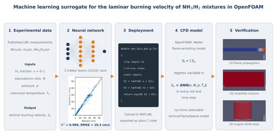
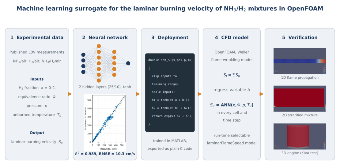
The workflow consists of five steps (Figure 1): (1) compiling published LBV measurements and defining physically motivated input variables; (2) training and cross-validating an ANN surrogate; (3) exporting the trained network as plain C code; (4) implementing this code as a laminar flame speed model in the premixed combustion solver of OpenFOAM; and (5) verifying the implementation in test cases of increasing complexity. Steps 1–3 were carried out in MATLAB [29], and steps 4 and 5 in OpenFOAM [30].
Figure 1.
Workflow of this study: from published measurements of the laminar burning velocity to a neural network surrogate that is deployed as C code in the OpenFOAM premixed combustion model and verified in 1D, 2D, and 3D test cases.
2.2. Experimental Data and Input Variables
The training data are 1445 published LBV measurements for NH3/air, H2/air, and NH3/H2/air mixtures, compiled from the literature in our previous work [22], which builds on the compilation of Üstün et al. [18]. Four implausible data points were excluded from the evaluation in Section 3.1: one H2/air point at 6 bar and Φ = 1 with Su = 531 cm/s, and three H2/air points at 350 K and 1 bar with Su = 30–44 cm/s, which are inconsistent with all other H2/air data and probably belong to an NH3/H2 blend. No synthetic data from kinetic simulations were added, because the surrogate is meant to represent measured flame behaviour and to be independent of the choice of reaction mechanism. The LBV is described as a function of four input variables (Table 1). The hydrogen fraction x is the volume fraction of H2 in the NH3/H2 fuel, and the equivalence ratio Φ is the ratio of the actual to the stoichiometric fuel–air ratio, with a stoichiometric oxygen demand of 0.75 mol O2 per mol NH3 and 0.5 mol O2 per mol H2. The dependence of the LBV on these variables changes strongly with the mixing ratio, and pure H2 and pure NH3 behave very differently.
Table 1.
Input and output variables and their ranges in the training dataset.
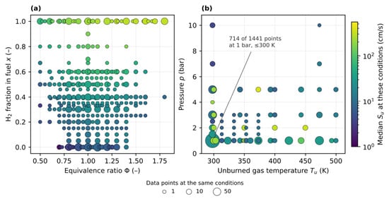
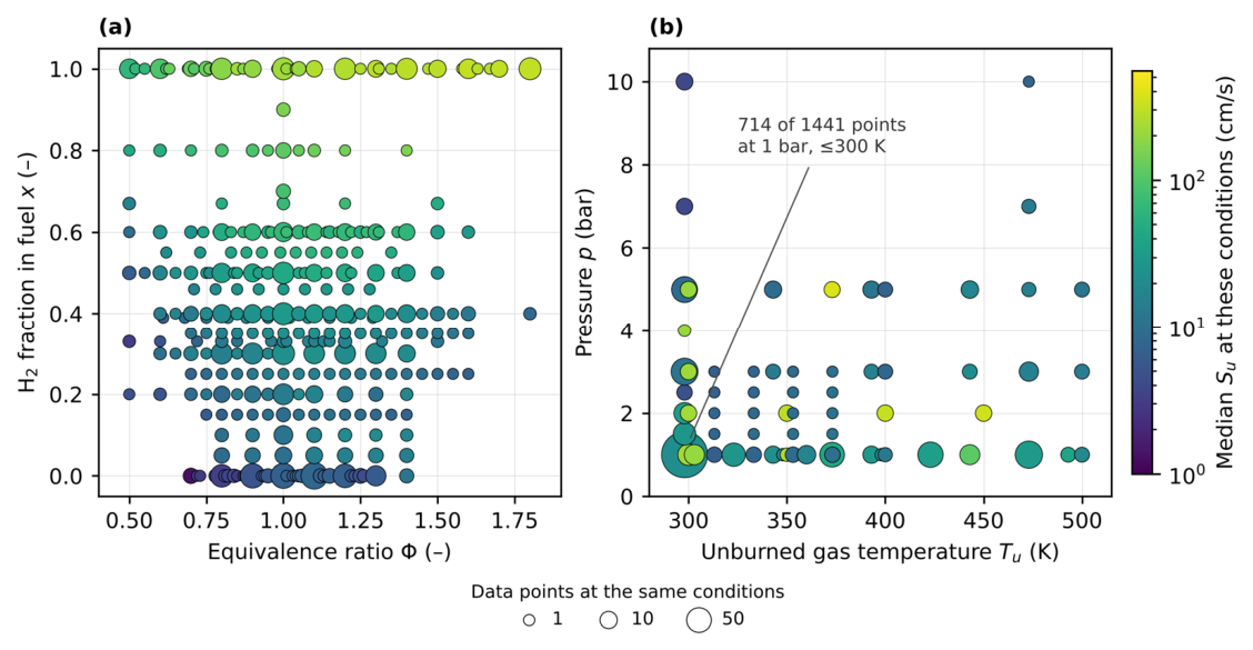
Measured data are challenging for ML algorithms. The data points are unevenly distributed in the parameter space, the values contain measurement errors, and the different measurement methods are not fully compatible [9,18]. Figure 2 shows the distribution of the data. Half of the measurements (714 of 1441) were taken at 1 bar and at most 300 K, and pure NH3 (338 points) and pure H2 (277 points) make up 43% of the data, whereas rich mixtures (Φ > 1.4, 102 points, of which 43 at Φ > 1.6), pressures above 5 bar (22 points), and hydrogen fractions between 0.6 and 1 (35 points) are sparsely covered. These regions are therefore analysed separately in Section 3.1. The choice of input variables is important. Physical and chemical insight was incorporated by using the hydrogen fraction of the fuel and the equivalence ratio instead of the molar fractions of NH3, H2, O2, and N2. Because the LBV spans more than two orders of magnitude, its natural logarithm was used as the training target, and all inputs were scaled to the interval [0, 1] using the minimum and maximum of the training data, as in [18].
Figure 2.
Distribution of the 1441 data points in the input space: (a) hydrogen fraction versus equivalence ratio, (b) pressure versus unburned gas temperature. Marker size indicates the number of data points at the same conditions, and colour the median measured laminar burning velocity.
2.3. Neural Network Architecture and Training
Several ML methods were tested, with GPR and ANN performing best, in agreement with [18,22]. For deployment in CFD, the ANN was chosen: its prediction requires only a fixed number of multiplications and additions, whereas a GPR prediction scales with the number of training points. The network is a fully connected feedforward network with four inputs, two hidden layers with 25 and 10 neurons, and one output (Table 2). With the vector of scaled inputs û, the prediction reads
where W1 (25 × 4), W2 (10 × 25), and w3 (10 × 1) are the weight matrices; c1, c2, and c3 are the bias vectors; and σ is the hyperbolic tangent activation function. The network has 396 trainable parameters. The hyperbolic tangent yields a smooth, continuously differentiable dependence of Su on the inputs, which avoids kinks in the burning velocity field of the CFD simulation, and the logarithmic output guarantees positive burning velocities.
Table 2.
Settings of the neural network and its training.
The network was trained with the MATLAB function fitrnet [29] with hyperbolic tangent activation, which minimises the mean squared error of ln Su with the limited-memory Broyden–Fletcher–Goldfarb–Shanno (L-BFGS) algorithm [31], without regularisation. Training stopped after at most 1000 iterations or when the relative change in the loss, the gradient, or the step fell below 10−6. The architecture was selected by varying the number of layers (1–3) and neurons per layer (5–50) and choosing the smallest network whose cross-validated error was within 8% of the best one. Performance was assessed by five-fold cross-validation: the data were randomly divided into five folds, each fold was predicted by a network trained on the other four, and the accuracy was evaluated using the coefficient of determination and the root-mean-square error.
where Su,i is the measured and Ŝu,i the predicted value of data point i;
u is the mean of the measurements; and N is the number of data points. Both metrics are evaluated for Su in cm/s, i.e., after back-transformation from the logarithm. The four implausible data points described in Section 2.2 were excluded from the evaluation. The final network used in CFD was trained on all data with the selected settings.
2.4. Premixed Combustion Model and Governing Equations
Premixed turbulent combustion is described by the flame-wrinkling model of Weller et al. [32], as implemented in the XiFluid solver module of OpenFOAM 13 [30]. The solver integrates the Favre-averaged conservation equations of mass and momentum,
where ρ is the density, U is the velocity field, p is the pressure, and τeff is the effective stress tensor, including the turbulent stresses from the turbulence model. Energy is described by transport equations for the total enthalpy and for the enthalpy of the unburned gas, from which the burned and unburned gas temperatures are obtained [30]. The flame position is tracked by the regress variable b (b = 1 unburned, b = 0 burned), which obeys the transport equation
where ρu is the density of the unburned gas, Dt is the turbulent diffusivity, and Su is the laminar burning velocity of the unburned gas. The interaction between turbulence and the flame front is represented by the flame-wrinkling factor Ξ, which is defined as the ratio of the turbulent to the laminar burning velocity,
St = Ξ Su.
In the transport model used here, Ξ obeys, in simplified form, the equation
where Ûs is the velocity of the flame surface, and the generation rate G and the removal rate R are chosen so that Ξ relaxes towards the equilibrium value [32,33]
where u′ is the turbulence intensity and Rη the Kolmogorov–Reynolds number.
The LBV thus enters both the source term of the b equation and the closure for Ξ, and it must be evaluated in every cell and time step from the local hydrogen fraction, equivalence ratio, pressure, and unburned gas temperature. OpenFOAM offers a constant value or algebraic correlations depending on stoichiometry, pressure, and temperature, such as the Gülder correlation [34]; alternatively, tables can be computed from chemical kinetics. Correlations are inaccurate outside their calibration range, especially for NH3/H2 blends [10,11], and kinetics-based tables are computationally expensive to generate and to interpolate in several dimensions. An ML model evaluated directly in the solver is an efficient alternative.
2.5. Implementation in OpenFOAM
The trained network was exported as a single C function containing the input scaling, the weights and biases of both hidden layers as constant arrays, the hyperbolic tangent activations, and the back-transformation of the output. This function has no dependencies beyond the C standard library. In OpenFOAM 13, it was wrapped in a new class derived from the abstract base class laminarFlameSpeed, which also underlies the built-in constant, Gülder, and Ravi–Petersen models. The class is registered in the run-time selection table, compiled with wmake into a shared library, and loaded through the libs entry of the controlDict file. It is selected in the combustionProperties dictionary with the entry laminarFlameSpeedCorrelation ANN, so that the solver itself is not modified. For every call, the model receives the cell fields of pressure and unburned gas temperature from the thermophysical model and the equivalence ratio, either as a constant for homogeneous mixtures or computed cell-wise from the fuel mass fraction for inhomogeneous mixtures. It loops over all cells and boundary faces and returns the field of Su.
The hydrogen fraction x is a run-time parameter of the model in the present version and is constant in space and time. Because the network was trained on the full range of x, any blend from pure NH3 to pure H2 can be selected for a simulation without retraining. A spatially and temporally varying hydrogen fraction requires an additional transport equation, which is discussed in Section 4. The model is therefore applicable only to mixtures with a uniform NH3/H2 ratio, in which the equivalence ratio may vary, but not to separate injection of the two fuels, in situ cracking, or strong preferential diffusion of H2. Because ∂ln Su/∂x ≈ 3.4–4.3 (Φ = 1, x = 0.3–0.95), a local deviation of x by ±0.03 already changes Su by 10%, i.e., by the scatter of the measurements.
To prevent uncontrolled extrapolation, all inputs are limited to the range of the training data before they are passed to the network (superscript *). Above the upper limits of temperature and pressure, the burning velocity at the limit is extrapolated with a power law,
where the exponents are the local logarithmic slopes of the network at the respective limit, αT = ∂ln Su/∂ln Tu at Tu = Tu,max and αp = ∂ln Su/∂ln p at p = pmax, evaluated for the current x and Φ. This choice makes the extrapolation continuous at the boundary and consistent with the trend of the data. For orientation, kinetic simulations for x = 0.6 and Φ = 1 at 300 K imply αp ≈ −0.37 between 1 and 5 bar [35], and the Gülder correlation uses temperature exponents of 1.56–2.0 and pressure exponents of −0.5 to −0.2 for hydrocarbon fuels [34]. Below the lower limits and for x and Φ, the inputs are clipped. The number of cells outside the training range is counted and written to the log file in every time step, so that the user can judge whether a simulation relies on extrapolated values.
Because the network is small, one evaluation requires about 400 multiply–add operations and 35 evaluations of the hyperbolic tangent, whose cost is quantified in Section 3.5.
For comparison, two alternative burning velocity models were used in the same solver. The first is the Gülder correlation built into OpenFOAM [34], Su = W Φη exp[−ξ (Φ − 1.075)2] (Tu/T0)α (p/p0)β, with T0 = 300 K and p0 = 1 bar, whose coefficients W, η, ξ, α, and β were fitted to the measurements for the selected hydrogen fraction. The second is a lookup table of Su over equivalence ratio, pressure, and unburned gas temperature for the selected hydrogen fraction, which was generated from the trained network on a grid of 27 × 42 × 19 points (Φ, Tu, p) and is interpolated trilinearly.
2.6. Test Cases and Numerical Setup
The implementation was verified with three test cases of increasing complexity (Table 3). The 1D case is a straight channel of 50 mm length with a uniform premixed mixture, ignited at the inlet (Table 3), which checks the implementation directly because the burning velocity and the wrinkling factor are uniform, so that the flame propagates at Ξ Su relative to the unburned gas. The 2D case is a rectangular domain of 70 mm × 35 mm bounded by symmetry planes, i.e., one quarter of a closed vessel, with a stratified mixture, richer in the lower half, and ignition in the lower left corner, which checks the response to local equivalence ratio, pressure, and temperature. It is based on the XiFluid tutorial moriyoshiHomogeneous [36]. The 3D case is the KIVA test engine of the XiFluid tutorials [36], with a homogeneous premixed charge, which demonstrates the use in a transient application with a moving mesh. The grid has 27,544 active cells and a compression ratio of 8.85, which we computed from the cell volumes at bottom dead centre (631 cm3) and the displacement (560 cm3). Instead of the tutorial values (1 bar, 373 K), the initial state was set to 0.6 bar and 300 K, representing throttled part load, so that the cylinder pressure remains within the pressure range of the training data until ignition.
Table 3.
Numerical setup of the test cases.
Following the OpenFOAM tutorials [36], the regress variable and the mixture fraction were convected with the bounded limitedLinear01 scheme, the enthalpies with the limitedLinear scheme, and, in the 3D case, velocity and turbulence quantities with the upwind scheme; diffusive terms used central differencing with limited non-orthogonal correction, and time was discretised with the implicit Euler scheme. Pressure–velocity coupling used the PIMPLE algorithm with two pressure correctors. In every corrector, the linear systems were solved to an absolute tolerance of 10−6 for pressure and 10−5 for all other variables, without relative tolerance in the final corrector. Grid independence was assessed for the 1D and 2D cases with three successively refined grids (Section 3.2).
3. Results
3.1. Accuracy of the Neural Network
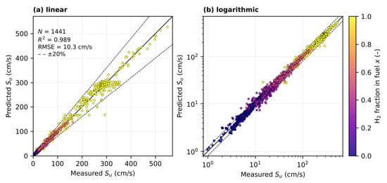
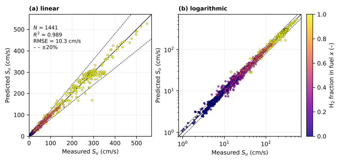
The network reaches R2 = 0.989 and RMSE = 10.3 cm/s on the 1441 data points, with a mean absolute error of 4.6 cm/s and a mean relative error of 8.4% (Figure 3). Most predictions lie within ±20% of the measurements. Table 4 breaks the error down by sub-range. In absolute terms, the error is largest for pure H2 (RMSE = 22.8 cm/s), where the burning velocity is highest; in relative terms, it is largest for lean mixtures with Φ < 0.8 (16.7%). At elevated pressure and temperature, the errors are small despite the sparse data (7.2% for p > 1 bar and 5.9% for Tu > 400 K). To quantify the scatter between experiments, the 676 data points that were measured at the same conditions as at least one other point were analysed. Their pooled standard deviation is 13.1 cm/s, or 6.8% on average. Even the mean of the measurements at each condition, which is the best possible deterministic prediction, has an RMSE of 11.1 cm/s for these points, compared with 13.1 cm/s for the network. The error of the network is therefore close to the scatter of the data. For comparison, GPR trained and evaluated on the same folds reached R2 = 0.988 and RMSE = 10.7 cm/s. On a similar experimental dataset of 1178 points, Üstün et al. [18] reported R2 = 0.976–0.988 and RMSE = 10.9–12.0 cm/s for neural networks and R2 = 0.983 and RMSE = 11.4 cm/s for GPR, evaluated on a fixed test subset.
Figure 3.
Predicted versus measured laminar burning velocity of the ANN for the 1441 data points on (a) linear and (b) logarithmic axes. Colour indicates the hydrogen fraction, and the dashed lines mark deviations of ±20%.
Table 4.
Error of the neural network with respect to the measurements by sub-range of the data.
The high absolute RMSE for pure H2 is not caused by a systematic bias of the network. Its relative error (8.4%) equals that of the other sub-ranges, and grouped by the predicted value, the mean deviation lies between −4.0% and +1.1% in all classes above 50 cm/s. The apparent underprediction of the highest measured values (−6% for 300–400 cm/s) is a regression-to-the-mean effect of the scatter: at 1 bar and 298 K, single measurements at Φ = 1.4–1.8 range from 252 to 354 cm/s, while the network reproduces the means at each condition within −3.4% to +5.6%. For the 149 pure-H2 points measured at repeated conditions, even these condition means have an RMSE of 23.4 cm/s, compared with 27.6 cm/s for the network.
To quantify the prediction uncertainty, ten replicas of the network (same architecture and scaling, RMSE = 10.0–10.3 cm/s) were retrained from different initial weights in Python 3.13 (scikit-learn 1.9.1), and ten networks per cross-validation fold were trained on bootstrap samples. Combined with the scatter of repeated measurements (standard deviation of ln Su of 0.09–0.17, depending on Φ), the bootstrap spread gives a 95% prediction interval that contained 91–100% of the held-out measurements in all sub-ranges in Table 4. Where data are dense, the interval spans a factor of about 1.25 (1.46 for Φ < 0.8). In the sparse sub-ranges, it widens to a factor of 1.6 for p > 5 bar and to a factor of 2.3–3.4 for p = 5–10 bar combined with x > 0.6 or Φ > 1.4 (14–37 data points, nearly all at 5 bar), where equally accurate replicas differ by 22–24%. Predictions in these sub-ranges are therefore estimates with an uncertainty of a factor of two or more.
3.2. One-Dimensional Flame Propagation and Grid Independence
The 1D case verifies the programming and implementation. A premixed mixture at uniform composition, pressure, and temperature is ignited at one end of a straight channel, so the LBV is constant throughout the domain (Figure 4). The propagation speed of the flame front, determined from the motion of the b = 0.5 isoline relative to the unburned gas, therefore corresponds to the value returned by the network multiplied by the wrinkling factor Ξ, i.e., 150 cm/s. On the medium grid, the computed propagation speed is 143.5 cm/s (Table 5), 4% below this value. The flame front is smeared over several cells because of the spatial discretisation, but its speed remains constant.
Figure 4.
One-dimensional test case: regress variable b (colour scale from 0, blue, burned, to 1, red, unburned) during flame propagation at constant laminar burning velocity.
Table 5.
Grid independence of the 1D and 2D test cases.
Table 5 shows the grid independence study. Refining the grid from 100 to 400 cells changes the propagation speed by less than 1%. For the 2D case, the burnout time changes by less than 1% between the medium and the fine grid.
3.3. Two-Dimensional Stratified Mixture
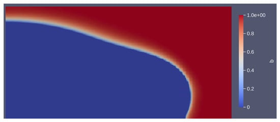
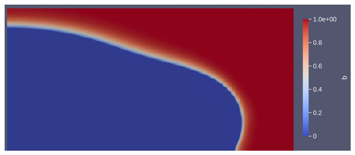
The 2D case checks the dependence on stoichiometry, temperature, and pressure. The closed domain is initialised with a non-uniform fuel–air mixture, with more fuel in the lower part than in the upper part (Figure 5). Ignition starts in the lower left corner. As combustion proceeds, temperature and pressure rise throughout the domain, so the unburned gas ahead of the flame is compressed and heated. Since the network returns a different LBV for each local combination of Φ, p, and Tu, the flame front progresses unevenly. The flame advances faster in the lower zone, whose equivalence ratio is closer to the maximum of the LBV, and the local Su at the flame front rises from 190 cm/s to 430 cm/s as pressure and unburned gas temperature increase from 1.2 bar to 7 bar and 300 K to 500 K.
Figure 5.
Two-dimensional test case with stratified fuel–air mixture (richer at the bottom); ignition in the lower left corner. Colour: regress variable b from 0 (blue, burned) to 1 (red, unburned).
3.4. Three-Dimensional Engine Case
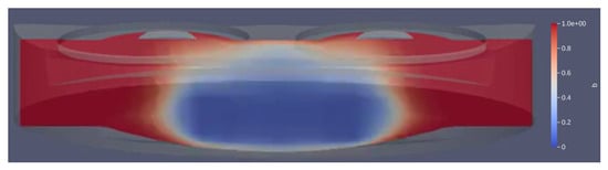
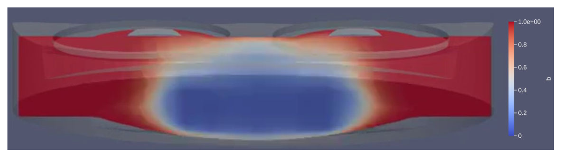
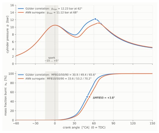
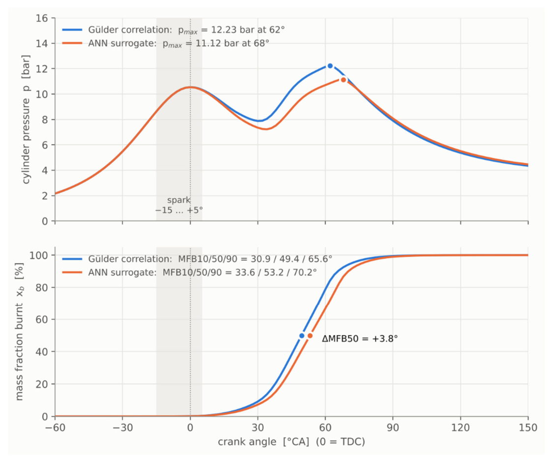
The 3D case is a transient application based on the KIVA test geometry distributed with OpenFOAM: a homogeneous premixed fuel–air mixture in the cylinder of a spark-ignition engine (Figure 6). During the compression stroke, pressure and temperature increase. At a specified piston position the mixture is ignited, and the flame propagates through the moving domain. The LBV is evaluated in every cell and time step from the instantaneous pressure and unburned gas temperature, which change continuously during compression and combustion. Figure 7 compares the cylinder pressure and the burned mass fraction obtained with the network and with the Gülder correlation; the lookup table, which was generated from the network, gives nearly identical results to the network. The Gülder correlation agrees with the network during the early flame development but predicts faster combustion in the phase of higher pressure and temperature: the peak pressure is 12.2 bar at 62 °CA after top dead centre with the correlation and 11.1 bar at 68 °CA with the network, 50% of the mass is burned at 49.4 °CA and 53.2 °CA, and the combustion duration (10–90% burned) is 34.7 °CA and 36.6 °CA, respectively. This is consistent with the structure of the correlation: its temperature and pressure exponents are constant, whereas the network and the table reproduce the dependence of these exponents on equivalence ratio and hydrogen fraction contained in the data. Because the training data are limited to 500 K and 10 bar, the cylinder pressure at ignition is within the training range, but the unburned gas temperature locally exceeds 500 K during the late compression stroke and the combustion phase, and the pressure exceeds 10 bar during combustion. The burning velocity is therefore obtained from the extrapolation of Equation (10) in 7% of the evaluations during combustion. The 3D case thus demonstrates the robustness of the coupling in a moving-mesh engine simulation, but not the accuracy of the surrogate at engine conditions, which requires training data at higher temperatures.
Figure 6.
Three-dimensional engine test case (KIVA test geometry): regress variable b in the cylinder with homogeneous premixed charge (colour scale from 0, blue, burned, to 1, red, unburned).
Figure 7.
Three-dimensional engine case: cylinder pressure and burned mass fraction over crank angle with the neural network and the Gülder correlation.
The sensitivity to the 7% extrapolated evaluations was assessed offline with the ten replicas at end-gas states of the engine case (x = 0.3, Φ = 1). At the boundary of the data (10 bar, 500 K), the replicas differ by a factor of 2.4 (16–38 cm/s), because no measurements exist for this combination. At 12 bar and 600 K, extrapolation with the local slopes of Equation (10) gives 18–96 cm/s, bounded exponents (1.5 ≤ αT ≤ 2.5, −0.5 ≤ αp ≤ 0) give 22–60 cm/s, and the literature exponents of Section 2.5 (αT = 1.8, αp = −0.37) give 21–50 cm/s, whereas clipping keeps the boundary value. The burning velocity in the extrapolated cells is therefore uncertain by about a factor of two, and bounded exponents are recommended.
The use of the unstretched LBV in the Weller model causes two further errors. Flame stretch κ changes the burning velocity approximately to Su − Lbκ, with the Markstein length Lb; this error decreases inversely with the kernel radius and mainly affects the early flame development. Thermodiffusive instabilities increase the flame speed of lean hydrogen-rich flames by factors of 1–4, increasingly with decreasing Φ and increasing pressure [37,38]. For NH3/H2 blends, direct numerical simulations give a stretch factor (enhancement of the local burning rate) of about 3 for x = 0.81 and Φ = 0.44 but about 1 for x = 0.43 and Φ = 0.95, and local shifts in Φ at the flame front by −0.2 to +0.1 [38], which change Su by −30% to +9% according to the network. For the present cases, this error vanishes in the planar 1D case, is limited to the kernel phase in the near-stoichiometric 3D case, and is small at the near-stoichiometric flame front of the 2D case, but it can dominate for lean mixtures with high hydrogen fractions.
3.5. Computing Time
Table 6 compares the three burning velocity models. The Gülder correlation needs the least computing time; compared with the correlation, the lookup table increases the total computing time by about 15% and the neural network by about 30%. The additional cost of the network results from the matrix–vector products and the evaluations of the hyperbolic tangent in every cell and time step; nevertheless, the evaluation of the burning velocity remains a smaller part of the total cost, which is dominated by the solution of the transport and pressure equations.
Table 6.
Comparison of the laminar burning velocity models in the OpenFOAM simulations.
To separate the cost of the burning velocity submodule from that of the pressure and transport equations, the three models were also timed in a stand-alone C benchmark for the 27,544 cells of the engine grid (one core, 2.8 GHz). One evaluation takes 42 ns for the Gülder correlation, 21 ns for the trilinear table, and 920 ns for the network (1000 ns including the input guard), i.e., 1.2, 0.6, and 25–28 ms per evaluation of the field. About 80% of the network cost is due to the 35 evaluations of the hyperbolic tangent; computing it from the exponential function halves the cost without changing the results. Because the table alone is cheaper than the correlation, the differences in total computing time also contain effects of the solution procedure and of the implementation, not only the cost of the submodule.
4. Discussion
The results show that an ML surrogate trained on experimental data can replace algebraic correlations or kinetics-based tables for the LBV in a standard CFD combustion model with little implementation effort. The workflow, consisting of training in MATLAB, export as C source code, and implementation as a run-time selectable model, uses generally available tools and does not require coupling a deep learning library to the solver, in contrast to platforms such as DeepFlame [24,25]. It is closest to the approach of Ambrutis and Povilaitis [23] for H2/air. The increments of the present work are the extension to a two-fuel system with the blend ratio as an additional input, training exclusively on measurements instead of a mixed experimental–synthetic dataset, the guard against extrapolation, and the quantitative verification including computing times. The dataset builds on the published compilation of [18], which makes the results comparable with the literature.
Accuracy and data. The ANN reached R2 = 0.989 and RMSE = 10.3 cm/s. This is comparable to the neural networks of Üstün et al. [18], who reported R2 = 0.976–0.988 and RMSE = 10.9–12.0 cm/s on 1178 experimental points, although the present network is deliberately small (25/10 neurons, 396 parameters), because it is evaluated in every cell and time step. Higher values were obtained only after adding 5890 synthetic points from 1D simulations (R2 = 0.999 [18]) or after removing 66 of 553 points as outliers (R2 > 0.99 [19]). The remaining error is of the order of the scatter between experiments (Section 3.1), which sets a lower limit for any model trained on measurements. The largest absolute errors occur for pure H2, where both the burning velocity and the scatter between experiments are largest. For many CFD applications, an error of this order is comparable to the uncertainty of the turbulent combustion model itself. The GPR model trained on the same folds achieved similar accuracy (Section 3.1) and is more robust for small datasets [22], but its prediction cost grows with the size of the training set, so the ANN is the better choice for evaluation in every cell and time step. Adding data from a validated mechanism would raise R2, but it would also transfer the uncertainties of that mechanism into the surrogate.
Validity range. An ML model is reliable only within the range of its training data. Outside this range, the tanh neurons saturate, so that the network tends towards constant values and does not reproduce the physical trends, for instance the increase in the burning velocity at the high unburned gas temperatures reached late in the compression stroke of an engine. The input guard of Section 2.5 makes the behaviour outside the training range explicit and controllable, and the logged number of out-of-range cells shows how strongly a simulation relies on extrapolation. The 3D engine case shows that this is not an academic concern: because the experimental data end at 500 K, 7% of the evaluations during combustion had to be extrapolated. Because the data are concentrated near atmospheric conditions (Figure 2), the sub-range errors in Table 4 should be consulted before applying the model to rich or high-pressure conditions. Augmenting the data with 1D simulations at engine-relevant conditions, as in [18], is one remedy.
Model limitations. The Weller model uses the unstretched LBV. Lean hydrogen-rich flames are affected by flame stretch and thermodiffusive instabilities, which the present closure does not represent. This limitation is shared by all LBV-based closures with a Ξ equation and is not specific to the ML surrogate. For lean mixtures with high hydrogen fractions, the results should therefore be regarded as qualitative. Two extensions are possible within the same framework: training a second output for the Markstein length, for which measurements of NH3/H2 flames exist, and combining it with Ξ closures that include Markstein-number effects, which are available in OpenFOAM. Likewise, the constant hydrogen fraction restricts the present model to mixtures with a fixed blend ratio, such as premixed charges from an upstream cracker or blending unit.
Comparison with correlation and lookup table. The network and the lookup table gave nearly identical engine results, while the Gülder correlation predicted faster combustion and an about 10% higher peak pressure. The correlation has two structural disadvantages. First, it describes the burning velocity only through the equivalence ratio, pressure, and temperature, with fuel-specific coefficients; the composition of the fuel, here the hydrogen fraction, and other concentrations such as dilution are not inputs and can only be considered by refitting the coefficients. Second, it imposes power laws with constant exponents, whereas measurements of NH3/H2 flames show that the temperature and pressure sensitivity changes with equivalence ratio and hydrogen fraction [10,11], so that such dependencies are captured only approximately. Both the network and the table represent these dependencies directly.
Computational cost. Little has been published on the cost of ML-based LBV models inside a CFD solver. Ambrutis and Povilaitis [23] found that a large DNN needed about 45 s for 106 predictions, compared with less than 1 s for the Malet correlation, whereas a reduced network showed no significant difference in flameFoam. Lookup tables are usually at least as fast as neural networks, because retrieval requires only a few memory accesses and an interpolation; in a flamelet application, simulations with unoptimised networks were 40–100 times slower than with the table [26]. The present results agree with this picture: compared with the correlation, the table increased the total computing time by about 15% and the small network by about 30%, while the network is about four orders of magnitude faster than 1D kinetic simulations [18]. The advantage of networks over tables lies in memory and in the number of inputs, because table size grows exponentially with the number of input variables [27,28]. For the three inputs in the present table, memory is not limiting, but each additional variable, such as a transported hydrogen fraction or dilution, multiplies the table size.
Best practice. From these results, the following recommendations can be derived for the choice of the burning velocity model in CFD. If a validated chemical mechanism is available, the burning velocity can be computed with 1D simulations and stored in a lookup table, which is faster than the network (Table 6). If no validated mechanism is available, as is still the case for many NH3/H2 conditions, a neural network trained on measurements is the method of choice, because it represents the measured dependencies on all inputs, including the fuel composition, without an assumed functional form. If computing time is critical, the trained network can itself be used to generate a lookup table, which combines the measurement basis of the network with the speed of tabulation. Algebraic correlations remain useful for quick estimates within their calibration range, but they do not account for the fuel composition and represent the temperature and pressure dependence only approximately.
Outlook. Three extensions follow directly. First, additional transport equations for the mixture composition will allow varying NH3/H2 ratios, for example from partial ammonia cracking or stratified injection. Second, the same workflow can predict further output variables such as the Markstein length, ignition delay time, or NOx formation, which is critical for ammonia combustion. Third, the method can be transferred to other fuels and fuel blends for which measurements exist but reliable mechanisms or correlations do not. Uncertainty estimates from GPR or network ensembles could additionally flag predictions outside the reliable range and guide new experiments through active learning [22].
5. Conclusions
To the author’s knowledge, this study presents the first implementation of a measurement-based machine learning surrogate for the laminar burning velocity of ammonia–hydrogen–air mixtures in a CFD combustion model. A neural network with two hidden layers of 25 and 10 neurons and hyperbolic tangent activation, trained on 1445 published measurements with the hydrogen fraction and the equivalence ratio as inputs and the logarithm of the burning velocity as output, reaches R2 = 0.989 and RMSE = 10.3 cm/s over the full range of hydrogen fractions, which is close to the scatter between experiments; the largest absolute errors occur for pure H2 and the largest relative errors for lean mixtures. Exported as plain C code, the network was implemented as a run-time selectable laminar flame speed model in OpenFOAM with a guard that limits the inputs to the training range and extrapolates temperature and pressure effects with a power law.
Coupled with the Weller flame-wrinkling model, the surrogate reproduced the prescribed burning velocity in the 1D case on a grid-independent mesh, responded consistently to local stoichiometry, pressure, and temperature in the 2D stratified case, and ran stably in the 3D engine case, although 7% of the burning velocity evaluations during combustion had to be extrapolated beyond the training range of 500 K and 10 bar. In the engine case, the network and a lookup table gave nearly identical results, whereas the Gülder correlation predicted faster combustion and an about 10% higher peak pressure, because it does not account for the fuel composition and represents the temperature and pressure dependence only approximately. Compared with the correlation, the table increased the total computing time by about 15% and the network by about 30%. As best practice, neural networks trained on measurements are recommended when no validated chemical mechanism is available, and lookup tables, generated from such a network or from a mechanism, when computing time is critical. The accuracy is limited by the uneven distribution and uncertainty of the experimental data, by the training range, and by the use of the unstretched burning velocity, which restricts quantitative predictions for lean hydrogen-rich flames. Future work will extend the training data to engine-relevant temperatures and pressures, add a transport equation for the hydrogen fraction, extend the surrogate to Markstein lengths and NOx formation, validate the coupled model against engine and burner experiments, and apply the workflow to other fuels.
Funding
This research received no external funding.
Data Availability Statement
The experimental data used for training are available from the publications compiled in [18,22]. The trained model and the OpenFOAM implementation are available from the author on request.
Conflicts of Interest
The author declares no conflicts of interest.
Abbreviations
The following symbols and abbreviations are used in this manuscript:
| b | Regress variable (1 unburned, 0 burned) |
| c1, c2, c3 | Bias vectors and output bias of the network |
| Dt | Turbulent diffusivity (m2/s) |
| G, R | Generation and removal rates of Ξ (1/s) |
| i | Index of the data point |
| k | Turbulent kinetic energy (m2/s2) |
| L | Length of the 1D domain (m) |
| N | Number of data points |
| p | Pressure (bar) |
| R2 | Coefficient of determination |
| Rη | Kolmogorov–Reynolds number |
| St | Turbulent burning velocity (m/s) |
| Su | Laminar burning velocity of the unburned gas (cm/s) |
| Su,ANN | Laminar burning velocity predicted by the network (cm/s) |
| Ŝu | Predicted laminar burning velocity (cm/s) |
| S̄u | Mean of the measured laminar burning velocities (cm/s) |
| T0, p0 | Reference temperature (300 K) and pressure (1 bar) of the Gülder correlation |
| Tu | Unburned gas temperature (K) |
| t | Time (s) |
| U | Velocity field (m/s) |
| Ûs | Velocity of the flame surface (m/s) |
| u′ | Turbulence intensity (m/s) |
| û | Vector of scaled network inputs |
| W | Coefficient of the Gülder correlation (cm/s) |
| W1, W2, w3 | Weight matrices and output weight vector of the network |
| x | Volume fraction of H2 in the fuel |
| αT, αp | Temperature and pressure exponents of the extrapolation |
| α, β | Temperature and pressure exponents of the Gülder correlation |
| ε | Dissipation rate of turbulent kinetic energy (m2/s3) |
| η, ξ | Coefficients of the Gülder correlation |
| Ξ, Ξeq | Flame-wrinkling factor and its equilibrium value |
| ρ, ρu | Density and density of the unburned gas (kg/m3) |
| σ | Activation function (hyperbolic tangent) |
| τeff | Effective stress tensor (Pa) |
| Φ | Equivalence ratio |
| * | Superscript: input limited to the training range |
| ANN | Artificial neural network |
| CFD | Computational fluid dynamics |
| DNN | Deep neural network |
| GPR | Gaussian process regression |
| LBV | Laminar burning velocity |
| L-BFGS | Limited-memory Broyden–Fletcher–Goldfarb–Shanno algorithm |
| LES | Large-eddy simulation |
| ML | Machine learning |
| NOx | Nitrogen oxides |
| RAS | Reynolds-averaged simulation |
| RMSE | Root-mean-square error |
| °CA | Degree crank angle |
References
- Kobayashi, H.; Hayakawa, A.; Somarathne, K.D.K.A.; Okafor, E.C. Science and technology of ammonia combustion. Proc. Combust. Inst. 2019, 37, 109–133. [Google Scholar] [CrossRef] [Scilit]
- Valera-Medina, A.; Xiao, H.; Owen-Jones, M.; David, W.I.F.; Bowen, P.J. Ammonia for power. Prog. Energy Combust. Sci. 2018, 69, 63–102. [Google Scholar] [CrossRef] [Scilit]
- Yang, J.; Li, Y. Effective and realistic strategies for large-scale liquid hydrogen production. Cryo 2025, 1, 8. [Google Scholar] [CrossRef] [Scilit]
- Yang, X.; Xiao, Z.; Hu, R.; Feng, D. A review on laminar burning velocity of ammonia flames. Energies 2025, 18, 6000. [Google Scholar] [CrossRef] [Scilit]
- Sahami, M.; Ghassemi, H.; Terziev, A.; Fikiin, K.; Stankov, B.; Pitchurov, G.; Ivanov, M. A CFD model for the evaporation of sub-micron droplet sprays across normal shocks. Thermo 2026, 6, 15. [Google Scholar] [CrossRef] [Scilit]
- Sahami, M.; Terziev, A.; Pitchurov, G.; Ivanov, M.; Fiaschi, D. Modeling the non-premixed combustion of methane enriched by hydrogen in a cylindrical combustor. Hydrogen 2026, 7, 132. [Google Scholar] [CrossRef] [Scilit]
- Li, J.; Huang, H.; Kobayashi, N.; Wang, C.; Yuan, H. Numerical study on laminar burning velocity and ignition delay time of ammonia flame with hydrogen addition. Energy 2017, 126, 796–809. [Google Scholar] [CrossRef] [Scilit]
- Lhuillier, C.; Brequigny, P.; Lamoureux, N.; Contino, F.; Mounaïm-Rousselle, C. Experimental investigation on laminar burning velocities of ammonia/hydrogen/air mixtures at elevated temperatures. Fuel 2020, 263, 116653. [Google Scholar] [CrossRef] [Scilit]
- Konnov, A.A.; Mohammad, A.; Kishore, V.R.; Kim, N.I.; Prathap, C.; Kumar, S. A comprehensive review of measurements and data analysis of laminar burning velocities for various fuel+air mixtures. Prog. Energy Combust. Sci. 2018, 68, 197–267. [Google Scholar] [CrossRef] [Scilit]
- Goldmann, A.; Dinkelacker, F. Approximation of laminar flame characteristics on premixed ammonia/hydrogen/nitrogen/air mixtures at elevated temperatures and pressures. Fuel 2018, 224, 366–378. [Google Scholar] [CrossRef] [Scilit]
- Pessina, V.; Berni, F.; Fontanesi, S.; Stagni, A.; Mehl, M. Laminar flame speed correlations of ammonia/hydrogen mixtures at high pressure and temperature for combustion modeling applications. Int. J. Hydrogen Energy 2022, 47, 25780–25794. [Google Scholar] [CrossRef] [Scilit]
- Ihme, M.; Chung, W.T.; Mishra, A.A. Combustion machine learning: Principles, progress and prospects. Prog. Energy Combust. Sci. 2022, 91, 101010. [Google Scholar] [CrossRef] [Scilit]
- Üstün, C.E.; De Freitas, R.D.S.M.; Okafor, E.C.; Shahbakhti, M.; Jiang, X.; Paykani, A. Machine learning applications for predicting fuel ignition and flame properties: Current status and future perspectives. Energy Fuels 2025, 39, 13281–13314. [Google Scholar] [CrossRef] [Scilit]
- Mehra, R.K.; Duan, H.; Luo, S.; Ma, F. Laminar burning velocity of hydrogen and carbon-monoxide enriched natural gas (HyCONG): An experimental and artificial neural network study. Fuel 2019, 246, 476–490. [Google Scholar] [CrossRef] [Scilit]
- Malik, K.; Żbikowski, M.; Teodorczyk, A. Laminar burning velocity model based on deep neural network for hydrogen and propane with air. Energies 2020, 13, 3381. [Google Scholar] [CrossRef] [Scilit]
- Eckart, S.; Prieler, R.; Hochenauer, C.; Krause, H. Application and comparison of multiple machine learning techniques for the calculation of laminar burning velocity for hydrogen-methane mixtures. Therm. Sci. Eng. Prog. 2022, 32, 101306. [Google Scholar] [CrossRef] [Scilit]
- Shahpouri, S.; Norouzi, A.; Hayduk, C.; Fandakov, A.; Rezaei, R.; Koch, C.R.; Shahbakhti, M. Laminar flame speed modeling for low carbon fuels using methods of machine learning. Fuel 2023, 333, 126187. [Google Scholar] [CrossRef] [Scilit]
- Üstün, C.E.; Herfatmanesh, M.R.; Valera-Medina, A.; Paykani, A. Applying machine learning techniques to predict laminar burning velocity for ammonia/hydrogen/air mixtures. Energy AI 2023, 13, 100270. [Google Scholar] [CrossRef] [Scilit]
- Yue, W.; Zhang, B.; Zhang, S.; Wang, B.; Xia, Y.; Liang, Z. A deep learning model for predicting the laminar burning velocity of NH3/H2/air. Appl. Sci. 2024, 14, 9603. [Google Scholar] [CrossRef] [Scilit]
- Üstün, C.E.; Eckart, S.; Valera-Medina, A.; Paykani, A. Data-driven prediction of laminar burning velocity for ternary ammonia/hydrogen/methane/air premixed flames. Fuel 2024, 368, 131581. [Google Scholar] [CrossRef] [Scilit]
- Rao, A.; Li, W.; Abbasi, M.S.; Shahid, M.I.; Farhan, M.; Zulfiqar, S.; Chen, T.; Ma, F.; Li, X. Machine learning-enhanced combustion modeling for predicting laminar burning velocity of ammonia-hydrogen mixtures using improved reaction mechanisms. Energy 2025, 320, 135259. [Google Scholar] [CrossRef] [Scilit]
- Klepp, G.; Sharma, A.; Dörksen, H. Laminar burning velocity of ammonia-hydrogen mixtures predicted by machine learning. Chem. Ing. Tech. 2026, e70179. [Google Scholar] [CrossRef] [Scilit]
- Ambrutis, A.; Povilaitis, M. Development of a CFD-suitable deep neural network model for laminar burning velocity. Appl. Sci. 2022, 12, 7460. [Google Scholar] [CrossRef] [Scilit]
- Mao, R.; Lin, M.; Zhang, Y.; Zhang, T.; Xu, Z.-Q.J.; Chen, Z.X. DeepFlame: A deep learning empowered open-source platform for reacting flow simulations. Comput. Phys. Commun. 2023, 291, 108842. [Google Scholar] [CrossRef] [Scilit]
- Li, H.; Yang, R.; Zhang, M.; Mao, R.; Chen, Z.X. A comprehensive study on the accuracy and generalization of deep learning-generated chemical ODE integrators. arXiv 2023, arXiv:2312.16387. [Google Scholar] [CrossRef] [Scilit]
- Shadram, Z.; Nguyen, T.M.; Sideris, A.; Sirignano, W.A. Neural network flame closure for a turbulent combustor with unsteady pressure. arXiv 2020, arXiv:2005.14167. [Google Scholar] [CrossRef] [Scilit]
- Salunkhe, A.; Deighan, D.; DesJardin, P.E.; Chandola, V. ChemTab: A physics guided chemistry modeling framework. In Computational Science—ICCS 2022; Lecture Notes in Computer Science; Springer: Cham, Switzerland, 2022. [Google Scholar] [CrossRef] [Scilit]
- Armstrong, E.; Hewson, J.C.; Sutherland, J.C. Characterizing tradeoffs in memory, accuracy, and speed for chemistry tabulation techniques. Combust. Sci. Technol. 2023, 195, 2614–2633. [Google Scholar] [CrossRef] [Scilit]
- MATLAB, version R2025b; The MathWorks, Inc.: Natick, MA, USA, 2025. Available online: https://www.mathworks.com (accessed on 26 October 2026).
- Weller, H.G.; Tabor, G.; Jasak, H.; Fureby, C. A tensorial approach to computational continuum mechanics using object-oriented techniques. Comput. Phys. 1998, 12, 620–631. [Google Scholar] [CrossRef] [Scilit]
- Liu, D.C.; Nocedal, J. On the limited memory BFGS method for large scale optimization. Math. Program. 1989, 45, 503–528. [Google Scholar] [CrossRef] [Scilit]
- Weller, H.G.; Tabor, G.; Gosman, A.D.; Fureby, C. Application of a flame-wrinkling LES combustion model to a turbulent mixing layer. Symp. (Int.) Combust. 1998, 27, 899–907. [Google Scholar] [CrossRef] [Scilit]
- Gülder, Ö.L. Turbulent premixed flame propagation models for different combustion regimes. Symp. (Int.) Combust. 1991, 23, 743–750. [Google Scholar] [CrossRef] [Scilit]
- Gülder, Ö.L. Correlations of laminar combustion data for alternative S.I. engine fuels. In Proceedings of the West Coast International Meeting and Exposition, San Diego, CA, USA, 6 August 1984; p. 841000. [Google Scholar] [CrossRef] [Scilit] [PubMed]
- Bochicchio, F.; D’Amato, M.; Magi, V.; Viggiano, A. On the influence of H2 addition on NH3 laminar flame speed under engine-like conditions. Energies 2024, 17, 4181. [Google Scholar] [CrossRef] [Scilit]
- The OpenFOAM Foundation. OpenFOAM-13, Source Code and Tutorials. Available online: https://github.com/OpenFOAM/OpenFOAM-13 (accessed on 26 October 2026).
- Berger, L.; Attili, A.; Pitsch, H. Intrinsic instabilities in premixed hydrogen flames: Parametric variation of pressure, equivalence ratio, and temperature. Part 2: Non-linear regime and flame speed enhancement. Combust. Flame 2022, 240, 111936. [Google Scholar] [CrossRef] [Scilit]
- Gaucherand, J.; Laera, D.; Schulze-Netzer, C.; Poinsot, T. DNS of turbulent premixed ammonia/hydrogen flames: The impact of thermo-diffusive effects. Flow Turbul. Combust. 2024, 112, 587–614. [Google Scholar] [CrossRef] [Scilit]



Disclaimer/Publisher’s Note: The statements, opinions and data contained in all publications are solely those of the individual author(s) and contributor(s) and not of MDPI and/or the editor(s). MDPI and/or the editor(s) disclaim responsibility for any injury to people or property resulting from any ideas, methods, instructions or products referred to in the content. |
© 2026 by the author. Licensee MDPI, Basel, Switzerland. This article is an open access article distributed under the terms and conditions of the Creative Commons Attribution (CC BY) license.