


Abstract
Day-ahead photovoltaic (PV) forecasting must resolve the coexistence of a smooth diurnal generation envelope and shorter-scale fluctuations while providing uncertainty information suitable for operational decision making. This paper develops a multi-resolution Wavelet–CNN–LSTM framework for 24 h ahead PV power forecasting and evaluates it using a five-year PVGIS-derived dataset for a 334.116 MW Rabigh case study. The forecasting information set is restricted to the preceding 24 h of PV power and meteorological observations, together with deterministic target-day temporal variables. A validation study selects a Haar level-2 decomposition of PV history into , , and components, which are processed through parallel convolutional branches before recurrent fusion. The resulting network contains 87,032 trainable parameters. On the 2023 temporal evaluation period, the proposed model achieves an RMSE of 17.228 MW, , and a daylight RMSE of 24.636 MW, corresponding to 25.69% forecast skill relative to 24 h seasonal persistence. A 7-day moving-block bootstrap confirms clear RMSE reductions relative to persistence and XGBoost, while the intervals for LSTM and CNN–LSTM include zero, indicating statistically comparable performance among the strongest recurrent models. Probabilistic forecasts obtained from 100-pass Monte Carlo dropout yield daylight PICP = 0.9279, MPIW = 84.06 MW, and Winkler score = 122.08 for nominal 90% intervals; an independent conformal calibration set requires no additional widening of the neural interval. The results show that multi-resolution representation can improve squared-error performance without sacrificing model compactness, while calibrated uncertainty provides a complementary measure of forecast reliability.
1. Introduction
Large-scale photovoltaic generation is increasingly exposed to scheduling, balancing, and reserve decisions that must be taken before the actual solar resource is realized. In this setting, forecast quality is not determined only by average point accuracy; the temporal distribution of forecast errors and the reliability of the associated uncertainty estimates are equally important for system operation [1,2,3]. This challenge is particularly relevant in high-irradiance power systems such as Saudi Arabia, where rapid PV deployment is increasing the operational importance of short-term and day-ahead forecasting [4,5].
PV power exhibits a pronounced diurnal structure superimposed with variability over several temporal scales. Persistence and classical time-series models capture the dominant periodic component but often struggle with nonlinear and regime-dependent behavior [6,7]. Machine learning models, including tree-based ensemble methods, can represent nonlinear relationships between historical conditions and future output [8,9]. Recurrent neural networks, and especially long short-term memory (LSTM) models, further exploit temporal dependence in sequential data [10,11,12,13], while CNN–LSTM architectures introduce local feature extraction before recurrent integration [14,15,16].
A remaining challenge is that a single raw PV sequence mixes a slowly varying diurnal structure with faster fluctuations. Multi-resolution representations provide a natural way to separate these components before learning. Wavelet decomposition has therefore been combined with deep-learning models for renewable-energy forecasting [17]. Recent multiscale CNN–LSTM work has likewise shown that explicitly resolving information at different temporal scales can improve PV forecasting [18]. Yet, a more informative assessment of such hybrid models requires more than reporting the best test error: the information available at the forecast origin must be controlled, the contribution of the decomposition must be validated, and the uncertainty in model-to-model performance differences must be quantified.
Weather information is another central element of the day-ahead problem. Forecasting frameworks that incorporate NWP or corrected irradiance forecasts explicitly account for target-horizon atmospheric uncertainty [19]. When archived operational weather forecasts are unavailable, however, using realized target-day weather can create an unrealistically favorable information set. The present study therefore restricts the model to historical meteorological observations and deterministic target-day temporal variables, providing a causal benchmark that does not rely on realized future weather.
The second methodological requirement is uncertainty quantification. Point forecasts alone do not indicate whether a predicted day is routine or difficult. Monte Carlo (MC) dropout offers a practical way to obtain stochastic neural forecasts [20,21], whereas conformal calibration provides a data-driven mechanism for assessing and, when necessary, adjusting predictive intervals [22]. Combining these elements with time-series-aware statistical testing allows point accuracy and predictive reliability to be evaluated within one framework.
Motivated by these considerations, this paper develops a compact Wavelet–CNN–LSTM model for direct 24 h PV forecasting. Its contribution lies in the integration of four elements: (i) a validation-selected multi-resolution representation of historical PV power; (ii) a causal day-ahead information set based on historical observations; (iii) temporal statistical inference for model comparisons; and (iv) independently calibrated probabilistic forecasting. The framework is evaluated using a PVGIS-derived Rabigh dataset spanning 2019–2023 and is compared with 24 h seasonal persistence, LSTM, CNN–LSTM, and XGBoost baselines.
The specific contributions are as follows:
- (1)
- A Haar level-2 Wavelet–CNN–LSTM architecture that decomposes the historical PV sequence into , , and components and learns scale-specific features through parallel CNN branches before recurrent fusion.
- (2)
- A validation-driven representation study covering wavelet configuration, retained subbands, and training objective, providing direct evidence for the selected multi-resolution input rather than treating the DWT as an untested preprocessing step.
- (3)
- A statistically rigorous deterministic evaluation using forecast skill and a 7-day moving-block bootstrap for RMSE differences, thereby preserving the temporal dependence of day-ahead forecast errors.
- (4)
- A probabilistic forecasting layer combining MC dropout with an independent calibration subset and daylight-specific PICP, MPIW, and Winkler score.
2. Related Work
2.1. Day-Ahead PV Forecasting
Day-ahead PV forecasting spans physical, statistical, machine learning, and hybrid approaches. Persistence remains a useful reference because it preserves the previous day’s diurnal profile, while statistical models provide interpretable temporal baselines [6,23]. Tree-based learners and other nonlinear regressors can capture interactions among historical power, weather, and temporal covariates without an explicit dynamical model [8,9].
Sequence models have become particularly important for solar forecasting. LSTM networks model long-range temporal dependencies through gated recurrent states [10,11,12,13], and CNN–LSTM architectures add local feature extraction to the recurrent pipeline [14,15]. Xue et al. [18] demonstrated a multiscale CNN–LSTM formulation for photovoltaic microgrids, illustrating the benefit of exposing the learner to multiple temporal representations. Wavelet-enhanced models pursue a related objective by decomposing a signal into approximation and detail components before learning [17].
The relevance of structured deep learning extends beyond PV forecasting. Graph-attention and recurrent architectures have been used for real-time inertia estimation from PMU measurements [24,25], while learning-based state estimators have been developed to maintain accuracy under hidden adversarial attacks [26]. These applications illustrate a broader principle that also motivates the present work: power-system data often contain structure across multiple temporal or spatial scales, and architectures that expose this structure explicitly can improve learning efficiency.
2.2. Weather Information and Operational Forecasting
The meteorological information available at the forecast origin fundamentally shapes a day-ahead PV forecasting problem. Operational systems commonly rely on NWP or other weather forecasts for the target horizon. Dai et al. [19], for example, combined irradiance correction with weather-mode reliability decisions to improve day-ahead PV forecasts. Such approaches explicitly model the uncertainty of future atmospheric conditions.
The present study addresses a different information regime. Because archived NWP forecasts corresponding to the historical PVGIS record are not available, the model uses historical meteorological context rather than realized target-day weather. This formulation isolates the predictive value of historical PV dynamics and multi-resolution representation without granting access to future observed meteorology. The resulting benchmark is therefore complementary to, rather than a replacement for, NWP-driven operational forecasting.
2.3. Probabilistic Forecasting
Probabilistic solar forecasting has increasingly focused on the joint requirements of reliability and sharpness [2,27]. MC dropout approximates predictive uncertainty by retaining dropout during repeated inference passes [20,21]. Although MC dropout provides a practical predictive distribution, raw prediction intervals are not guaranteed to achieve their nominal empirical coverage and should therefore be assessed for calibration [22,27]. Conformal methods provide an additional layer of calibration by using held-out conformity scores to assess the required interval adjustment [22]. This separation between model fitting and interval calibration is adopted here through a dedicated chronological calibration period.
Taken together, the literature identifies three complementary needs in day-ahead PV forecasting: a representation able to resolve multi-scale temporal behavior, an information set that respects forecast-time availability, and uncertainty estimates that are evaluated for both coverage and sharpness. The proposed framework is designed around these three requirements.
3. Proposed Methodology
3.1. Study Area and Data
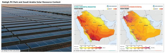
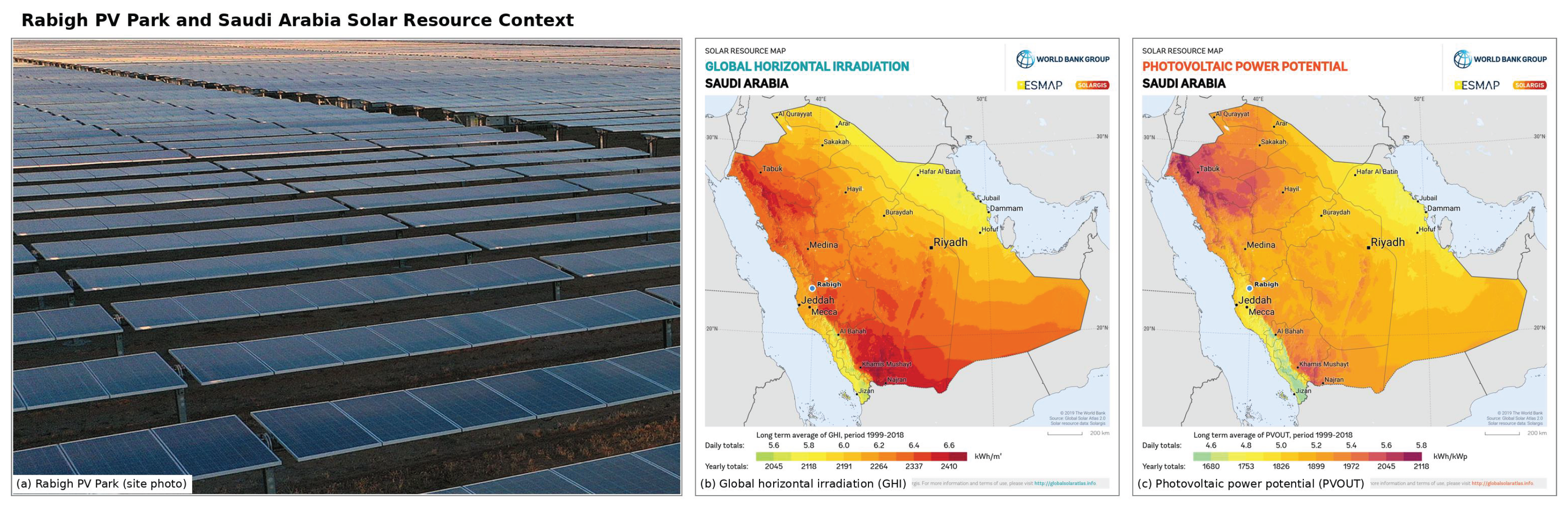
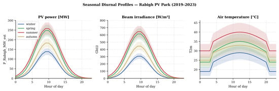
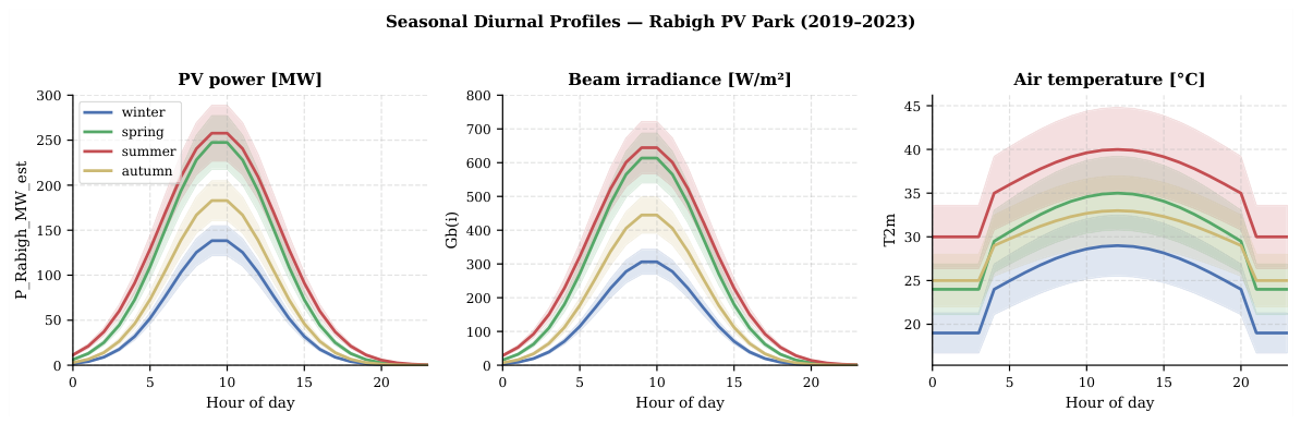
The case study is centred at approximately 22.80° N and 39.163° E near Rabigh on Saudi Arabia’s western Red Sea coast. The location and regional solar-resource context are shown in Figure 1. The site is characterized by a strong solar resource and marked seasonal variation (see Figure 2), providing a useful setting for evaluating day-ahead PV forecasting.
Figure 1.
Rabigh case-study location within the Saudi Arabian solar-resource context: (a) site image, (b) long-term global horizontal irradiation, and (c) photovoltaic power potential.
Figure 2.
Seasonal diurnal profiles of PV power, beam irradiance, and air temperature over the 2019–2023 record.
Hourly data for 2019–2023 were obtained from PVGIS (version 5.3) using the SARAH3 database [28,29]. The modeled PV system has a nominal capacity of 334.116 MW, crystalline-silicon technology, free mounting, optimal orientation, and 14% system loss. The target variable is PVGIS-estimated AC power, while the meteorological record includes beam irradiance , diffuse irradiance , ground-reflected irradiance , air temperature , wind speed , and solar height .
Before constructing forecasting windows, the hourly time index was verified for uniqueness and continuity, and the variables were screened against their physical bounds. Forecasting examples were formed only from complete contiguous sequences; no interpolation was introduced into the modeling pipeline. PV power was normalized by nominal capacity, and meteorological scaling parameters were estimated from the training period only. Deterministic cyclical temporal variables were used to encode hour-of-day and day-of-year information.
Table 1 summarizes the five-year record. The large difference between median and upper-percentile PV output reflects the expected combination of nighttime zeros and high daytime production and motivates the separate daylight evaluation later in the paper.
Table 1.
Summary statistics of hourly PVGIS-derived variables over 2019–2023. Nighttime observations are included.
3.2. Forecasting Problem and Chronological Protocol
At 00:00 local time, the model produces the complete 24 h PV profile for the target day,
The input consists of the previous 24 h of PV power and meteorological observations, together with deterministic temporal variables aligned with the target day. Realized target-day irradiance, temperature, and wind are not supplied to the model.
The data are partitioned chronologically to separate model fitting, model selection, interval calibration, and evaluation (Table 2). This separation is particularly important for probabilistic forecasting because the conformity scores must be estimated independently of model fitting.
Table 2.
Chronological experimental protocol.
3.3. Multi-Resolution PV Representation
For each forecast origin, the wavelet transform is applied only to the corresponding 24 h historical PV sequence. This window-local construction prevents future target values from influencing the decomposition. With the selected Haar level-2 representation,
where represents the low-frequency component of the historical PV profile and and represent progressively finer variations. The transform is implemented using the PyWavelets (v1.9.0) DWT multiresolution analysis with symmetric boundary extension [30]. All models were implemented in Python (v3.12) using TensorFlow/Keras (v2.19).
The representation was selected on VAL before the final model evaluation. The search considered alternative wavelet families, decomposition levels, historical contexts, subband combinations, and loss functions. Table 3 summarizes the two analyses most directly related to the final design. Removing any one of the three retained components degraded validation daylight RMSE. Among the evaluated training objectives, absolute-error loss produced the lowest validation daylight RMSE and was therefore used for model fitting.
Table 3.
Validation evidence supporting the selected wavelet representation and training objective.
3.4. Wavelet–CNN–LSTM Architecture
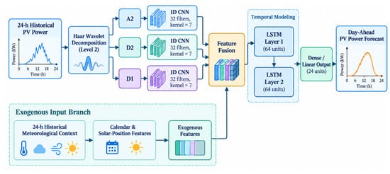
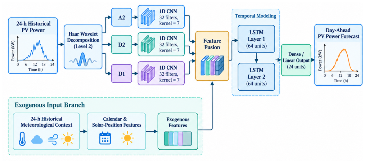
Figure 3 illustrates the proposed architecture. The three wavelet components are processed through parallel one-dimensional CNN branches with 32 filters and kernel size 7. Their learned representations are fused with a 24-step weather-and-calendar sequence and passed to two stacked LSTM layers with 64 units each. The model generates the complete 24 h PV forecast directly.
Figure 3.
Proposed Wavelet–CNN–LSTM architecture for direct 24 h PV power forecasting.
The final configuration is listed in Table 4. The network contains 87,032 trainable parameters, providing a compact recurrent model despite the parallel multi-resolution input representation.
Table 4.
Final Wavelet–CNN–LSTM configuration.
3.5. Baselines
Four baselines are used to place the proposed model in context. The 24 h seasonal persistence forecast uses the preceding day’s hourly PV profile. The LSTM baseline captures recurrent temporal dependence without convolutional or wavelet processing. The CNN–LSTM baseline introduces convolutional feature extraction but does not decompose the PV history. XGBoost (v3.1) [31] provides a non-recurrent nonlinear benchmark and is configured with 350 estimators, maximum depth 4, and learning rate 0.005. All models are evaluated against the same 2023 target sequence.
3.6. Probabilistic Forecasting
The deterministic Wavelet–CNN–LSTM is extended probabilistically by retaining dropout during inference and generating stochastic forecasts [20]. For a nominal 90% interval, the empirical 5th and 95th percentiles define the raw MC-dropout limits. Calibration is performed on CAL using the nonconformity score [22]
and finite-sample quantile . The calibrated interval becomes
For XGBoost, the calibration scores are based on absolute residuals, yielding a symmetric split-conformal interval.
4. Evaluation Framework
4.1. Deterministic Performance
Root mean square error is used as the primary point-forecast metric because it penalizes larger deviations more strongly, which is relevant for balancing and reserve decisions:
The coefficient of determination is
Forecast skill relative to seasonal persistence is defined as
Because deterministic nighttime zeros can mask differences among PV forecasting models, daylight RMSE is evaluated separately for .
4.2. Statistical Comparison
Model-to-model RMSE differences are quantified as
A positive value favors the proposed model. Confidence intervals are estimated using 5000 moving-block bootstrap replications with a 7-day block length, preserving short-range temporal dependence across adjacent forecasting days. A paired Wilcoxon signed-rank test applied to daily absolute-error summaries is reported as complementary evidence of distributional differences.
4.3. Probabilistic Performance
Prediction intervals are evaluated during daylight using three complementary measures of calibration and sharpness [2,32]. PICP measures empirical coverage,
while MPIW measures sharpness,
The Winkler score combines interval width with a penalty for misses,
Coverage is interpreted relative to the nominal 90% target; interval width is meaningful only jointly with coverage.
5. Results and Discussion
5.1. Overall Forecasting Performance
Table 5 summarizes deterministic performance over 2023. The Wavelet–CNN–LSTM achieves the lowest RMSE, 17.228 MW, and the highest , 0.9641. Its daylight RMSE is 24.636 MW. Relative to seasonal persistence, the reduction in RMSE is 25.69%, establishing that the model captures information beyond a repeated previous-day profile. Relative to XGBoost, the reduction is 20.12%, indicating a material advantage for explicit temporal representation in this experiment.
Table 5.
Deterministic forecasting performance over the 2023 evaluation period.
The comparison with the two recurrent baselines is more nuanced. The Wavelet–CNN–LSTM improves RMSE by 1.48% relative to LSTM and 0.74% relative to CNN–LSTM. These differences are small in absolute terms, suggesting that the principal value of the wavelet stage is not wholesale replacement of recurrent modeling but a modest redistribution of error through a more structured representation of PV history. This interpretation is examined further using horizon-dependent, seasonal, and statistical analyses.
5.2. Where the Multi-Resolution Representation Helps
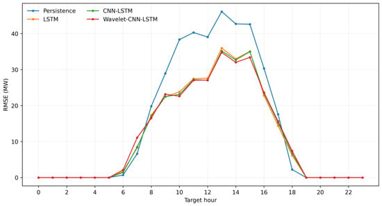
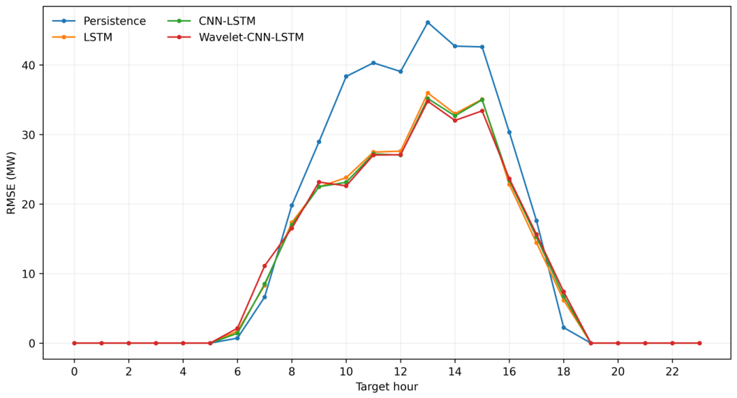
Forecast error varies strongly across the 24 target hours (Figure 4). The largest errors occur during the central daylight period, when absolute PV output is high and deviations contribute most strongly to annual RMSE. The Wavelet–CNN–LSTM achieves lower RMSE than both recurrent baselines at several of these high-output hours, including hours 10–15, while LSTM or CNN–LSTM remain better near some morning and evening transitions. The resulting pattern explains how a relatively small average difference can still lead to the lowest annual squared error.
Figure 4.
Target-hour RMSE for seasonal persistence and the recurrent neural models.
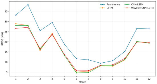
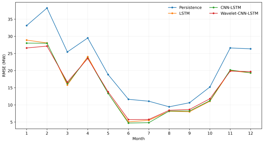
The monthly analysis reveals a related pattern (Figure 5). The proposed model performs particularly well in several of the higher-error months, including January and February, whereas LSTM or CNN–LSTM can be slightly better during lower-error summer periods. This behavior suggests that the multi-resolution representation is most useful when the historical PV trajectory contains stronger deviations from the regular diurnal pattern. It does not confer a uniform advantage under every operating condition.
Figure 5.
Monthly RMSE for seasonal persistence and the recurrent models.
This operating-regime dependence is consistent with the validation ablation in Table 3. Removing the low-frequency approximation or either detail component reduces validation performance, indicating that the three retained scales contribute complementary information. The result also aligns conceptually with multiscale CNN–LSTM forecasting [18], where explicitly resolving temporal scales improves feature extraction.
5.3. Statistical Evidence
The moving-block bootstrap provides a more rigorous interpretation of the numerical ranking. As shown in Table 6, the Wavelet–CNN–LSTM reduces RMSE relative to persistence by 5.955 MW, with a 95% confidence interval of [4.342, 7.478] MW. The corresponding reduction relative to XGBoost is 4.338 MW, with an interval of [3.119, 5.686] MW. Both intervals remain clearly above zero.
Table 6.
Statistical comparison against Wavelet–CNN–LSTM. Positive ΔRMSE denotes lower RMSE for the proposed model.
In contrast, the differences relative to LSTM and CNN–LSTM are 0.259 MW and 0.129 MW, with confidence intervals of [, 0.830] and [, 0.470] MW, respectively. These intervals include zero. Thus, the evidence supports a clear improvement over persistence and XGBoost, but not a statistically established RMSE advantage over the strongest recurrent baselines.
The Wilcoxon tests indicate that the paired daily absolute-error distributions differ, but the bootstrap intervals are more informative for the direction and magnitude of the RMSE comparison. This distinction is important: a small p-value does not imply that the proposed model dominates every baseline under every error criterion.
5.4. Probabilistic Forecasting
Table 7 reports the daylight performance of nominal 90% prediction intervals. MC dropout for the Wavelet–CNN–LSTM achieves PICP = 0.9279, slightly above the nominal target, with MPIW = 84.06 MW and Winkler score = 122.08. The XGBoost split-conformal interval is narrower (79.41 MW) but under-covers at 0.8690 and consequently has a higher Winkler score of 128.18.
Table 7.
Daylight probabilistic forecasting performance for nominal 90% prediction intervals.
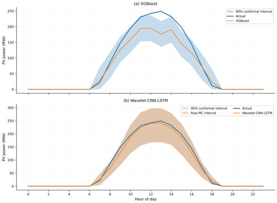
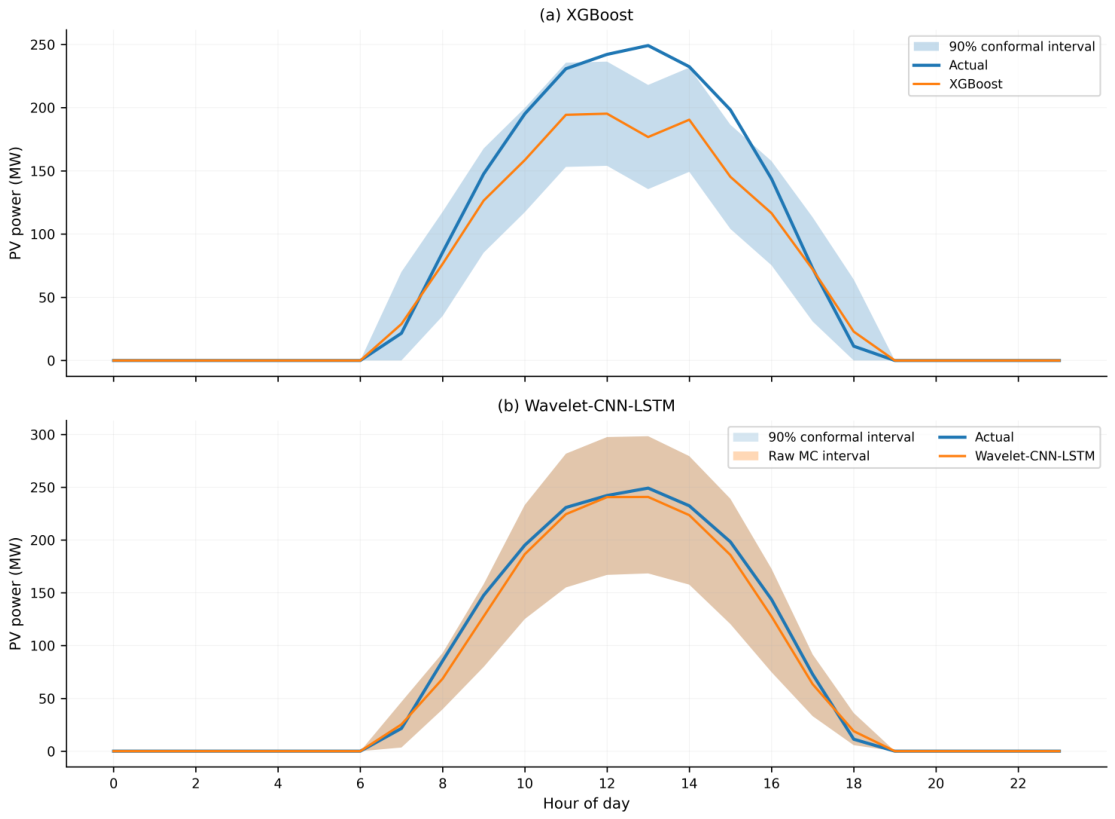
For the neural model, the calibration quantile is MW. Under the adopted conformity score, the raw MC-dropout intervals therefore required no additional widening on CAL. This result is informative in two ways. First, the stochastic network already generated an interval that was sufficiently conservative on the calibration period. Second, the test coverage of 92.8% shows that this conservatism persisted into 2023, albeit with modest overcoverage. The lower Winkler score relative to XGBoost indicates that the wider neural interval is compensated by improved coverage. Figure 6 illustrates representative 90% prediction intervals for XGBoost and Wavelet–CNN–LSTM, highlighting the differences in interval width and uncertainty characterization between the two approaches.
Figure 6.
Representative nominal 90% prediction intervals for XGBoost and Wavelet–CNN–LSTM.
6. Limitations and Future Work
The study has three principal limitations. First, the target is PVGIS-estimated AC power rather than measured SCADA production. Consequently, the benchmark does not fully represent plant-specific effects such as soiling, degradation, inverter behavior, equipment outages, maintenance, curtailment, or plant controls. Curtailment in particular can introduce time-dependent differences between available and delivered PV power [33]. Validation against measured plant output is therefore necessary before operational performance claims can be made.
Second, the forecasting information set does not include archived operational NWP forecasts. Restricting the model to historical meteorological observations avoids use of realized future weather, but it also means that the experiment does not represent the full information available to a modern day-ahead forecasting system. A natural next step is to evaluate the frozen architecture with archived NWP fields and compare the value of multi-resolution historical context under realistic weather-forecast uncertainty.
Third, the analysis is limited to one PVGIS-based location. For uncertainty quantification, rolling or adaptive conformal approaches are also worth investigating because seasonal changes can weaken the exchangeability assumptions of standard split-conformal calibration.
7. Conclusions
This paper developed a multi-resolution Wavelet–CNN–LSTM framework for direct 24 h PV power forecasting under a causal historical-information setting. A validation study selected a Haar level-2 decomposition of the preceding 24 h PV profile into , , and , and the resulting components were processed through parallel CNN branches before recurrent fusion with exogenous context.
On the 2023 temporal evaluation period, the model achieved an RMSE of 17.228 MW, , daylight RMSE of 24.636 MW, and 25.69% forecast skill relative to seasonal persistence. Moving-block bootstrap analysis showed clear RMSE reductions relative to persistence and XGBoost, while LSTM and CNN–LSTM remained statistically competitive. The probabilistic extension achieved daylight PICP = 0.9279 for nominal 90% intervals, together with MPIW = 84.06 MW and Winkler score = 122.08.
These results indicate that multi-resolution representation can improve squared-error performance without requiring a large network, while probabilistic forecasting adds information that point metrics alone cannot provide. The strongest next validation step is a frozen-model study using archived operational NWP forecasts and measured SCADA power across multiple PV sites.
Author Contributions
Conceptualisation, F.A. (Faisal Albeladi); methodology, F.A. (Faisal Albeladi) and M.E.D.; software, F.A. (Faisal Albeladi); formal analysis, F.A. (Faisal Albeladi) and M.A.; investigation, F.A. (Faisal Albeladi), M.A., and K.B.; writing—original draft, F.A. (Faisal Albeladi); writing—review and editing, M.E.D., M.A., K.B., A.A., and F.A. (Faisal Alhassani); supervision, F.A. (Faisal Albeladi); funding acquisition, F.A. (Faisal Albeladi). All authors have read and agreed to the published version of the manuscript.
Funding
This project was funded by the KAU Endowment (WAQF) at King Abdulaziz University, Jeddah, Saudi Arabia. The authors gratefully acknowledge WAQF and the Deanship of Scientific Research (DSR) for their technical and financial support.
Data Availability Statement
The PVGIS source data are publicly available from [28].
Conflicts of Interest
The authors declare no conflicts of interest.
Abbreviations
| PV | Photovoltaic |
| PVGIS | Photovoltaic Geographical Information System |
| DWT | Discrete wavelet transform |
| CNN | Convolutional neural network |
| LSTM | Long short-term memory |
| MC | Monte Carlo |
| PICP | Prediction interval coverage probability |
| MPIW | Mean prediction interval width |
| RMSE | Root mean square error |
| NWP | Numerical weather prediction |
| SCADA | Supervisory control and data acquisition |
| CAL | Calibration subset |
References
- International Renewable Energy Agency (IRENA). Renewable Power Generation Costs in 2023; Technical Report; IRENA: Abu Dhabi, United Arab Emirates, 2024. [Google Scholar]
- Lauret, P.; David, M.; Pedro, H.T.C. Probabilistic solar forecasting using quantile regression models. Energies 2017, 10, 1591. [Google Scholar] [CrossRef] [Scilit]
- Gandhi, O.; Zhang, W.; Kumar, D.S.; Rodriguez-Gallegos, C.D.; Yagli, G.M.; Yang, D.; Reindl, T.; Srinivasan, D. The value of solar forecasts and the cost of their errors: A review. Renew. Sustain. Energy Rev. 2024, 189, 113915. [Google Scholar] [CrossRef] [Scilit]
- Kingdom of Saudi Arabia Vision 2030. National Renewable Energy Program (NREP). Saudi Vision 2030 Secretariat, Riyadh, 2023. Available online: https://www.vision2030.gov.sa (accessed on 1 May 2026).
- Gherboudj, I.; Zorgati, M.; Chamarthi, P.K.; Tuomiranta, A.; Mohandes, B.; Beegum, N.S.; Al-Sudairi, J.; Al-Owain, O.; Shibli, H.; El-Moursi, M.; et al. Renewable energy management system for Saudi Arabia: Methodology and preliminary results. Renew. Sustain. Energy Rev. 2021, 149, 111334. [Google Scholar] [CrossRef] [Scilit]
- Inman, R.H.; Pedro, H.T.; Coimbra, C.F. Solar forecasting methods for renewable energy integration. Prog. Energy Combust. Sci. 2013, 39, 535–576. [Google Scholar] [CrossRef] [Scilit]
- Das, U.K.; Tey, K.S.; Seyedmahmoudian, M.; Mekhilef, S.; Idris, M.Y.I.; Van Deventer, W.; Horan, B.; Stojcevski, A. Forecasting of photovoltaic power generation and model optimization: A review. Renew. Sustain. Energy Rev. 2018, 81, 912–928. [Google Scholar] [CrossRef] [Scilit]
- Voyant, C.; Notton, G.; Kalogirou, S.; Nivet, M.L.; Paoli, C.; Motte, F.; Fouilloy, A. Machine learning methods for solar radiation forecasting: A review. Renew. Energy 2017, 105, 569–582. [Google Scholar] [CrossRef] [Scilit]
- Ahmad, M.W.; Mourshed, M.; Rezgui, Y. Tree-based ensemble methods for predicting PV power generation and their comparison with support vector regression. Energy 2018, 164, 465–474. [Google Scholar] [CrossRef] [Scilit]
- Hochreiter, S.; Schmidhuber, J. Long short-term memory. Neural Comput. 1997, 9, 1735–1780. [Google Scholar] [CrossRef] [Scilit] [PubMed]
- Wang, F.; Xuan, Z.; Zhen, Z.; Li, K.; Wang, T.; Shi, M. A day-ahead PV power forecasting method based on LSTM-RNN model and time correlation modification under partial daily pattern prediction framework. Energy Convers. Manag. 2020, 212, 112766. [Google Scholar] [CrossRef] [Scilit]
- Abdel-Nasser, M.; Mahmoud, K. Accurate photovoltaic power forecasting models using deep LSTM-based learning. Neural Comput. Appl. 2019, 31, 2727–2740. [Google Scholar] [CrossRef] [Scilit]
- Gao, M.; Li, J.; Hong, F.; Long, D. Day-ahead power forecasting in a large-scale photovoltaic plant based on weather classification using LSTM. Energy 2019, 187, 115838. [Google Scholar] [CrossRef] [Scilit]
- Tovar, M.; Robles, M.; Rashid, F. PV Power Prediction, Using CNN-LSTM Hybrid Neural Network Model. Case of Study: Temixco-Morelos, México. Energies 2020, 13, 6512. [Google Scholar] [CrossRef] [Scilit]
- Yu, D.; Choi, W.; Kim, M.; Liu, L. Forecasting Day-Ahead Hourly Photovoltaic Power Generation Using Convolutional Self-Attention Based Long Short-Term Memory. Energies 2020, 13, 4017. [Google Scholar] [CrossRef] [Scilit]
- Unlu, A.; Peña, M. Comparative Analysis of Hybrid Deep Learning Models for Electricity Load Forecasting During Extreme Weather. Energies 2025, 18, 3068. [Google Scholar] [CrossRef] [Scilit]
- Mishra, M.; Byomakesha Dash, P.; Nayak, J.; Naik, B.; Kumar Swain, S. Deep learning and wavelet transform integrated approach for short-term solar PV power prediction. Measurement 2020, 166, 108250. [Google Scholar] [CrossRef] [Scilit]
- Xue, H.; Ma, J.; Zhang, J.; Jin, P.; Wu, J.; Du, F. Power Forecasting for Photovoltaic Microgrid Based on MultiScale CNN-LSTM Network Models. Energies 2024, 17, 3877. [Google Scholar] [CrossRef] [Scilit]
- Dai, H.; Zhang, Y.; Wang, F. A Day-Ahead PV Power Forecasting Method Based on Irradiance Correction and Weather Mode Reliability Decision. Energies 2025, 18, 2809. [Google Scholar] [CrossRef] [Scilit]
- Gal, Y.; Ghahramani, Z. Dropout as a Bayesian approximation: Representing model uncertainty in deep learning. In Proceedings of the 33rd International Conference on Machine Learning (ICML), New York, NY, USA, 19–24 June 2016; pp. 1050–1059. [Google Scholar]
- Wang, K.; Du, H.; Jia, R.; Jia, H. Performance Comparison of Bayesian Deep Learning Model and Traditional Bayesian Neural Network in Short-Term PV Interval Prediction. Sustainability 2022, 14, 12683. [Google Scholar] [CrossRef] [Scilit]
- Angelopoulos, A.N.; Bates, S. Conformal Prediction: A Gentle Introduction. Found. Trends Mach. Learn. 2023, 16, 494–591. [Google Scholar] [CrossRef] [Scilit]
- Pedro, H.T.C.; Coimbra, C.F.M. Assessment of forecasting techniques for solar power production with no exogenous inputs. Sol. Energy 2012, 86, 2017–2028. [Google Scholar] [CrossRef] [Scilit]
- Albeladi, F.; Basulaiman, K.; Barati, M. Enhancing System Inertia Estimation: Multi-Head Graph Attention Networks Leveraging PMU Measurements. In Proceedings of the 2024 IEEE Texas Power and Energy Conference (TPEC), College Station, TX, USA, 12–13 February 2024; IEEE: New York, NY, USA, 2024; pp. 1–6. [Google Scholar] [CrossRef] [Scilit]
- Albeladi, F.; Basulaiman, K.; Barati, M. Beyond GCN: Accurate Real-Time Inertia Estimation With Multi-Head Spatial-Temporal Graph Attention Network Coupled With LSTM. IEEE Trans. Ind. Appl. 2026, 62, 5069–5078. [Google Scholar] [CrossRef] [Scilit]
- Basulaiman, K.; Albeladi, F.; Almutairi, F.M.; Saeed, A.; Barati, M. LBSCA: Learning Real-Time Power System State Estimation Under Hidden Adversarial Attacks. IEEE Access 2025, 13, 169340–169351. [Google Scholar] [CrossRef] [Scilit]
- Doubleday, K.; Van Scyoc-Hernandez, V.; Hodge, B.M. Benchmark probabilistic solar forecasts: Characteristics and recommendations. Sol. Energy 2020, 206, 52–67. [Google Scholar] [CrossRef] [Scilit]
- European Commission, Joint Research Centre. Photovoltaic Geographical Information System (PVGIS). 2024. Available online: https://joint-research-centre.ec.europa.eu/pvgis (accessed on 4 April 2025).
- Pfeifroth, U.; Druecke, J.; Kothe, S.; Trentmann, J.; Schroeder, M.; Hollmann, R. SARAH-3–satellite-based climate data records of surface solar radiation. Earth Syst. Sci. Data 2024, 16, 5243–5265. [Google Scholar] [CrossRef] [Scilit]
- Lee, G.R.; Gommers, R.; Wasilewski, F.; Wohlfahrt, K.; O’Leary, A. PyWavelets: A Python package for wavelet analysis. J. Open Source Softw. 2019, 4, 1237. [Google Scholar] [CrossRef] [Scilit]
- Chen, T.; Guestrin, C. XGBoost: A Scalable Tree Boosting System. In Proceedings of the 22nd ACM SIGKDD International Conference on Knowledge Discovery and Data Mining, San Francisco, CA, USA, 13–17 August 2016; pp. 785–794. [Google Scholar] [CrossRef] [Scilit]
- Gneiting, T.; Raftery, A.E. Strictly Proper Scoring Rules, Prediction, and Estimation. J. Am. Stat. Assoc. 2007, 102, 359–378. [Google Scholar] [CrossRef] [Scilit]
- Alduhaymi, M.; Alqahtani, M.H.; Kesici, M.; Albeladi, F.; Basulaiman, K. Time-series analysis of photovoltaic curtailment in radial distribution networks. Sustain. Energy Grids Netw. 2026, 47, 102430. [Google Scholar] [CrossRef] [Scilit]

Disclaimer/Publisher’s Note: The statements, opinions and data contained in all publications are solely those of the individual author(s) and contributor(s) and not of MDPI and/or the editor(s). MDPI and/or the editor(s) disclaim responsibility for any injury to people or property resulting from any ideas, methods, instructions or products referred to in the content. |
© 2026 by the authors. Licensee MDPI, Basel, Switzerland. This article is an open access article distributed under the terms and conditions of the Creative Commons Attribution (CC BY) license.