STR-GRU: A Spatio-Temporal Representation-Enhanced GRU for Short-Term Station-Level EV Charging Demand Forecasting

Abstract

Accurate short-term station-level electric vehicle (EV) charging demand forecasting is important for efficient charging-station operation and local grid management. However, several challenges remain. First, charging demand exhibits overall demand evolution and rapid short-term variations that are difficult to model simultaneously. Second, demand varies across spatially distinct stations and exhibits recurring intraday and weekly patterns, requiring effective spatio-temporal representations to capture such characteristics. Existing methods commonly combine graph-based inter-station modeling with temporal modeling, but uneven station distributions complicate inter-station modeling and general temporal modeling may not fully capture recurring patterns. Third, electricity price and temperature provide complementary information, but their predictive relevance can differ across stations. To address these challenges, we propose a Spatio-Temporal Representation-Enhanced GRU (STR-GRU). The proposed model includes three core modules: LD-GRU, STRE, and AEFF. The Level-Difference Dual-Branch GRU (LD-GRU) separately encodes demand levels and first-order differences to model overall demand evolution and short-term variations. Spatio-Temporal Representation Enhancement (STRE) uses learnable station, time-of-day, and day-of-week embeddings to represent demand differences across spatially distinct stations and recurring temporal patterns without inter-station graph construction or information propagation. Adaptive Exogenous Feature Fusion (AEFF) adaptively fuses electricity price and temperature according to station-specific demand representations to account for differences in their predictive relevance. Experiments on six urban charging networks and three forecasting horizons demonstrate competitive forecasting performance and a favorable accuracy–efficiency trade-off.

1. Introduction

The need to reduce fossil-fuel dependence and transport-related emissions has driven the transition toward low-carbon transportation [1]. Electric vehicles (EVs) play an important role in this transition. Growing EV adoption has increased charging demand and the need for effective deployment and operation of charging infrastructure [2]. Meanwhile, large-scale EV charging can increase load variability and pose operational challenges for local distribution networks [3]. Therefore, accurate short-term charging demand forecasts can support charging resource allocation, charging-station operation, local load management, and coordination between charging infrastructure and the power grid [4].

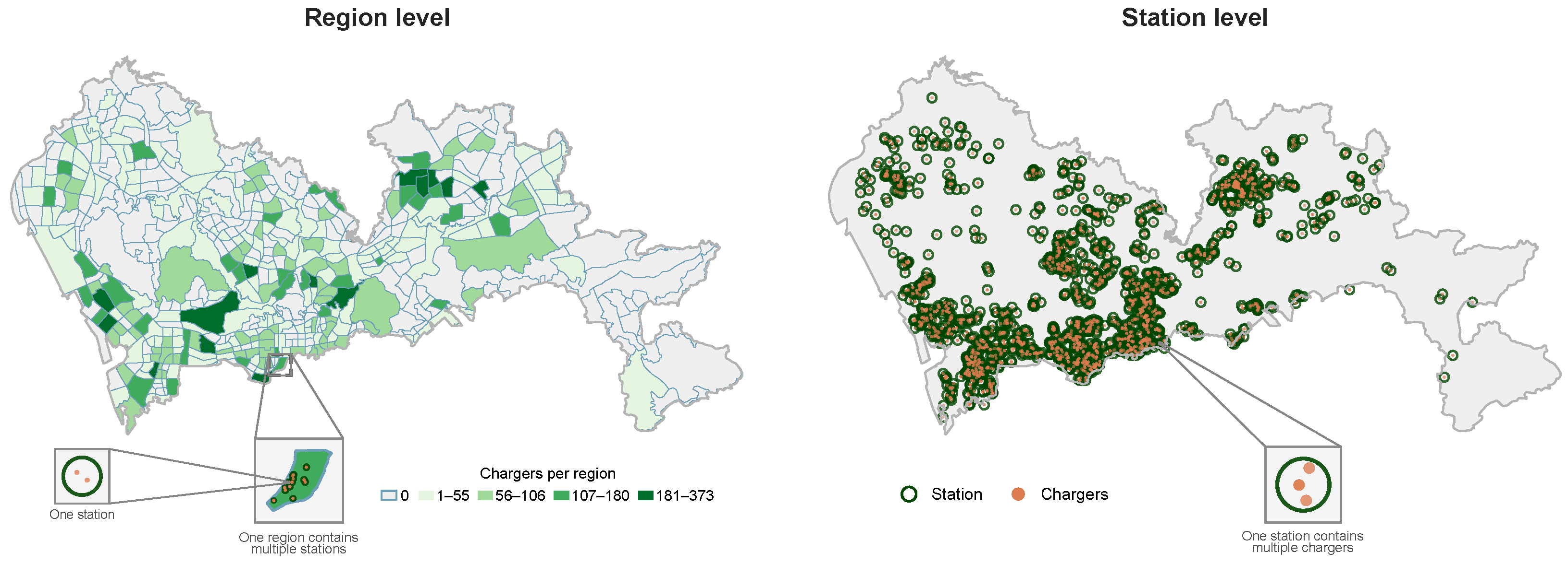
EV charging demand forecasting is commonly formulated at the regional and station levels [5,6]. As illustrated in Figure 1, regional-level forecasting predicts aggregated demand within spatial units containing multiple charging stations, whereas station-level forecasting predicts demand at individual stations. Regional studies typically partition urban areas into grids, traffic zones, or functional regions. Charging demand within these spatial units exhibits temporal dependencies, while demand across different units can exhibit spatial relationships. Accordingly, existing regional-level methods commonly combine temporal modeling with graph-based spatial modeling [7,8,9]. However, aggregating charging demand across spatial units can smooth local demand variations [10]. Such aggregation may limit the usefulness of regional forecasts for operational decisions that require station-specific demand information. In contrast, station-level forecasting treats each charging station as a distinct spatial entity and directly predicts its demand, providing finer-grained information for station operation and charging resource allocation.

Figure 1. Regional-level and station-level representations of EV charging demand forecasting.

At the station level, forecasting methods have gradually evolved from temporal modeling to spatio-temporal modeling by incorporating inter-station spatial relationships. Early studies mainly focused on temporal dependencies in historical charging observations. For example, Ma and Faye [11] combined LSTM-based temporal modeling with time-related features for multistep charging-station occupancy prediction, while Wang et al. [6] employed LSTM for short-term station-level charging demand forecasting. However, charging demand can exhibit spatial correlations across stations, motivating the joint modeling of temporal dependencies and inter-station spatial relationships. Accordingly, subsequent studies developed graph-based spatio-temporal models. Shi et al. [12] combined gated temporal convolution, spatio-temporal attention, and multi-graph convolution to capture temporal and spatial dependencies. Kim et al. [13] combined CBi-LSTM-based temporal modeling with graph convolution over spatial relationships derived from station attributes. More recently, Wang et al. [14] integrated adaptive graph learning and graph convolution with GRU to jointly capture inter-station correlations and temporal dependencies. Overall, these studies demonstrate the effectiveness of graph-based modeling for capturing inter-station spatial dependencies in station-level EV charging demand forecasting.

In addition to temporal dependencies and inter-station spatial relationships, exogenous variables can provide complementary predictive information for station-level EV charging demand forecasting. Among these variables, electricity price and temperature are particularly relevant to charging demand. Electricity price can influence charging decisions and charging patterns [15,16], while temperature is associated with vehicle energy consumption and charging behavior [17]. Accordingly, recent station-level forecasting studies have incorporated electricity price and temperature together with historical charging observations. For example, Cao et al. [18] incorporated regional electricity price, air temperature, and weather conditions as dynamic exogenous variables for charging demand forecasting at individual stations. Similarly, Yang et al. [19] considered time-of-use electricity price and temperature, together with other influencing factors, for EV charging-station load forecasting. These studies demonstrate the value of incorporating electricity price and temperature into station-level EV charging demand forecasting.

Despite these advances, several challenges remain in station-level EV charging demand forecasting. First, station-level charging demand exhibits both overall demand evolution and rapid short-term variations [20]. Existing temporal models can capture overall demand evolution, but rapid short-term variations remain difficult to model. Thus, accurately modeling both overall demand evolution and short-term variations remains challenging for short-term forecasting. Second, charging demand varies substantially across spatially distinct charging stations and also exhibits recurring intraday and weekly patterns [21]. This requires effective spatio-temporal representations that capture demand differences across spatially distinct stations and recurring temporal patterns. Graph-based methods commonly model inter-station spatial relationships and combine them with temporal modeling to learn such representations [14]. However, uneven station distributions complicate inter-station modeling [22], while recurring temporal patterns may not be fully captured by general temporal modeling. Therefore, effectively representing demand differences across spatially distinct stations and recurring temporal patterns remains challenging. Finally, electricity price and temperature provide complementary predictive information, but their predictive relevance can differ [19]. Previous studies commonly fuse exogenous variables directly with demand features [18,19]. Such fusion may not adequately account for differences in predictive relevance. Therefore, adaptively fusing exogenous variables remains challenging.

To address these challenges, we propose a Spatio-Temporal Representation-Enhanced GRU (STR-GRU) for short-term station-level EV charging demand forecasting. The proposed model consists of three core modules: the Level-Difference Dual-Branch GRU (LD-GRU), Spatio-Temporal Representation Enhancement (STRE), and Adaptive Exogenous Feature Fusion (AEFF). The main contributions are summarized as follows:

• We propose LD-GRU, which separately encodes historical demand levels and their first-order differences to model overall demand evolution and short-term variations.
• We develop STRE, which uses learnable station, time-of-day, and day-of-week embeddings to represent demand differences across spatially distinct stations and recurring temporal patterns without inter-station graph construction or information propagation.
• We develop AEFF, which adaptively fuses electricity price and temperature according to station-specific demand representations to account for differences in their predictive relevance across stations.
• Extensive experiments on six urban charging networks and three forecasting horizons demonstrate the competitive forecasting performance of STR-GRU and its favorable accuracy–efficiency trade-off.

The remainder of this paper is organized as follows. Section 2 reviews related work on EV charging demand forecasting. Section 3 presents STR-GRU. Section 4 reports the experimental setup and results. Section 5 discusses the findings and limitations. Finally, Section 6 concludes the paper and outlines future work.

2. Related Work

2.1. Temporal Modeling for EV Charging Demand Forecasting

Short-term EV charging demand forecasting requires effective modeling of temporal dependencies in historical charging observations. Statistical and machine learning methods have been widely used to model these temporal dependencies [23,24]. However, these methods have limited ability to model nonlinear and time-varying charging demand. Accordingly, deep learning methods have been increasingly used for short-term forecasting [4]. Among them, recurrent neural networks are widely used to model temporal dependencies. Ma and Faye [11] combined LSTM-based temporal modeling with time-related features for multistep charging-station occupancy prediction. Wang et al. [6] employed LSTM for short-term station-level charging demand forecasting. These studies show that recurrent models can effectively capture temporal dependencies from historical charging observations.

Although recurrent models can capture temporal dependencies, charging demand can also exhibit rapid variations over short time intervals [25]. This has led to the use of convolutional and hybrid methods for modeling local and multi-scale temporal patterns. Tian et al. [26] combined temporal convolution with recurrent modeling for short-term EV charging-load forecasting. Zhang et al. [25] employed multi-channel and temporal convolutions to model charging-load variations across different time scales. More recently, Cheng and Liu [27] incorporated feature extraction, frequency enhancement, and error correction for multistep charging-load forecasting. These methods extend temporal modeling from sequential dependencies to short-term and multi-scale demand variations.

Despite these advances, station-level charging demand exhibits both overall demand evolution and rapid short-term variations. These characteristics place different requirements on temporal modeling and can be difficult to model simultaneously. Thus, accurately modeling both overall demand evolution and short-term variations remains challenging for short-term station-level EV charging demand forecasting.

2.2. Spatio-Temporal Modeling for Station-Level EV Charging Demand Forecasting

Beyond temporal dynamics, station-level charging demand varies substantially across spatially distinct stations and also exhibits recurring intraday and weekly patterns [28]. These characteristics require effective spatio-temporal representations that capture demand differences across spatially distinct stations and recurring temporal patterns. Existing studies have developed different ways to learn such representations. A common approach is to combine inter-station spatial modeling with temporal modeling through graph-based methods.

Graph-based methods often construct inter-station relationships from predefined station information. Shi et al. [12] proposed STMGCN, which combines gated temporal convolution, spatio-temporal attention, and multi-graph convolution to capture temporal and spatial dependencies. Kim and Kim [13] combined CBi-LSTM-based temporal modeling with graph convolution over spatial relationships derived from station attributes. Other studies have used additional spatial information to construct inter-station relationships. Xie et al. [29] constructed multiple graphs from geographic distance, transportation networks, and traffic density. Hou et al. [30] used station location and historical load information to model inter-station relationships. These methods provide effective ways to incorporate predefined spatial information, but their spatial modeling depends on inter-station relationships specified in advance. To reduce this dependence, more recent studies have learned inter-station relationships directly from data. Wang et al. [14] proposed ASTGRN, which learns inter-station correlations from historical charging observations through adaptive graph learning. The learned relationships are then combined with graph convolution and GRU-based temporal modeling. Compared with predefined graphs, adaptive graph learning reduces the need to manually define inter-station relationships. However, both predefined and adaptive graph methods still model spatial information through inter-station graphs and information propagation [12,14].

Recent studies have also considered information associated with individual stations and recurring temporal patterns. Dai and Shi [20] incorporated station identifiers together with hour-of-day and day-of-week information into station-level spatio-temporal forecasting. A related representation approach has also been explored in general spatio-temporal forecasting. Shao et al. [31] proposed STID, which uses learnable spatial and temporal identity embeddings. Spatial identities distinguish individual nodes, while temporal identities represent recurring temporal patterns. Unlike graph-based methods, STID does not rely on inter-node graph construction or information propagation.

These studies provide different ways to learn spatio-temporal representations. Graph-based methods can effectively model inter-station spatial relationships, but uneven station distributions can complicate inter-station modeling [22]. Meanwhile, recurring temporal patterns may not be fully captured by general temporal modeling. Thus, effectively representing demand differences across spatially distinct stations and recurring temporal patterns remains challenging for station-level EV charging demand forecasting.

2.3. Exogenous Variable Modeling for EV Charging Demand Forecasting

EV charging demand is influenced not only by historical charging observations but also by exogenous variables. Among these variables, electricity price and temperature are particularly relevant to charging demand. Previous studies have examined their relationships with charging demand from different perspectives. Bao et al. [15] investigated temporal and spatial price elasticities of public charging demand. Kuang et al. [16] further analyzed heterogeneous price responses and spatial spillover effects across charging areas. For temperature, weather-related studies have examined the effects of weather conditions on EV charging load [17]. These findings show that electricity price and temperature can provide complementary information for charging demand forecasting.

Based on these findings, forecasting studies have incorporated exogenous variables together with historical charging observations. Cao et al. [18] incorporated regional electricity price, air temperature, and weather conditions into station-level charging demand forecasting. Yang et al. [19] considered time-of-use electricity price, temperature, and other influencing factors for charging-station load forecasting. Beyond feature incorporation, more structured methods have also been developed to use exogenous information. PIAST [7] modeled price–demand relationships and spatial spillover effects within a physics-informed citywide forecasting framework. At the station level, Dai and Shi [20] integrated historical observations, station attributes, periodic information, and exogenous variables within a multi-source spatio-temporal framework. These studies show that exogenous information can be incorporated through different modeling strategies in charging demand forecasting.

Different exogenous variables can have different predictive relevance [19]. Existing studies have used feature selection and feature enhancement to incorporate such information [18,19]. However, these methods do not adapt exogenous feature fusion to station-specific demand characteristics. Thus, effectively integrating exogenous variables with different predictive relevance remains challenging for station-level EV charging demand forecasting.

3. Methodology

This section formulates the station-level EV charging demand forecasting task and presents the proposed STR-GRU. STR-GRU consists of three main modules: Level-Difference Dual-Branch GRU (LD-GRU), Spatio-Temporal Representation Enhancement (STRE), and Adaptive Exogenous Feature Fusion (AEFF). We first formulate the forecasting task and introduce the overall architecture. We then describe the three modules in sequence, followed by the direct multi-step prediction head and model training procedure.

3.1. Problem Formulation

Consider an urban EV charging network containing N charging stations. Let ${\mathbf{x}}_t\in {\mathbb{R}}^N$ denote the charging demand observed at all stations at time step t. Given a historical window of P time steps, the historical demand sequence is defined as

$${\mathbf{X}}_{t-P+1:t}=[{\mathbf{x}}_{t-P+1},\dots ,{\mathbf{x}}_t]\in {\mathbb{R}}^{N\times P},$$

(1)

where P denotes the historical input length.

In addition to historical charging demand, electricity price and temperature are used as exogenous variables. Their historical sequences over the same input window are denoted by

$${\mathbf{Z}}_{t-P+1:t}^{\mathrm{price}},{\mathbf{Z}}_{t-P+1:t}^{\mathrm{temp}}\in {\mathbb{R}}^{N\times P}.$$

(2)

Given a forecasting horizon of H, the prediction target is

$${\mathbf{Y}}_{t+1:t+H}=[{\mathbf{x}}_{t+1},\dots ,{\mathbf{x}}_{t+H}]\in {\mathbb{R}}^{N\times H}.$$

(3)

Accordingly, the forecasting task is formulated as

$${\widehat{\mathbf{Y}}}_{t+1:t+H}=f_{\mathit{\theta }}\left({\mathbf{X}}_{t-P+1:t},{\mathbf{Z}}_{t-P+1:t}^{\mathrm{price}},{\mathbf{Z}}_{t-P+1:t}^{\mathrm{temp}}\right)$$

(4)

where $f_{\mathit{\theta }}(·)$ denotes the forecasting function and $\mathit{\theta }$ represents its trainable parameters.

3.2. Overall Architecture

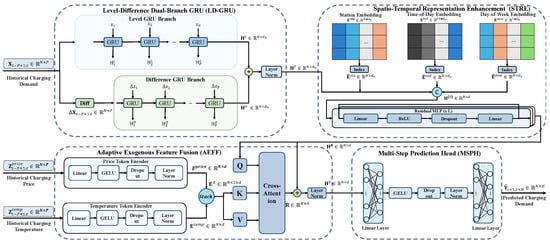
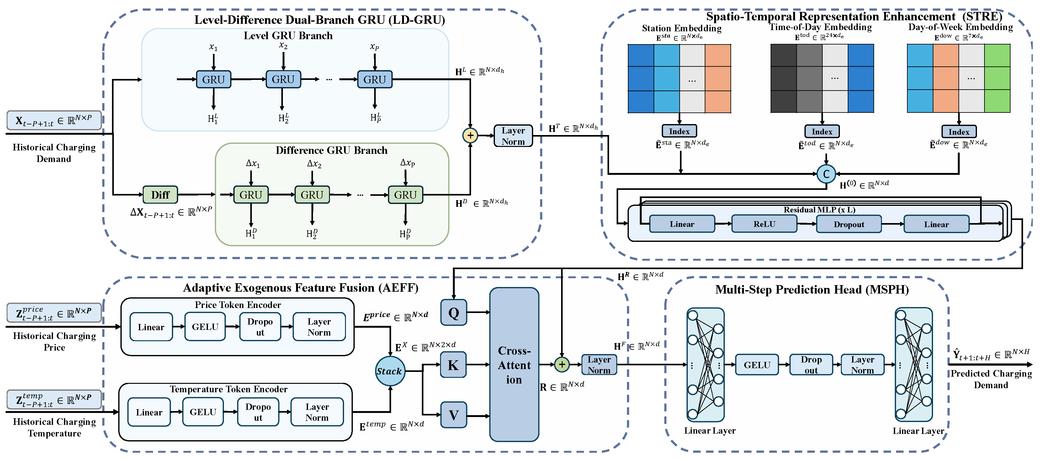
Figure 2 shows the overall architecture and data flow of STR-GRU. LD-GRU first separately encodes historical demand levels and first-order differences to model overall demand evolution and short-term variations, producing the temporal representation ${\mathbf{H}}^T$. STRE then combines ${\mathbf{H}}^T$ with station, time-of-day, and day-of-week embeddings to represent demand differences across spatially distinct stations and recurring temporal patterns, producing the enhanced spatio-temporal representation ${\mathbf{H}}^R$. Based on ${\mathbf{H}}^R$, AEFF adaptively fuses electricity price and temperature according to station-specific demand representations to account for differences in their predictive relevance across stations, producing the fused representation ${\mathbf{H}}^F$. Finally, the prediction head maps ${\mathbf{H}}^F$ directly to the future H time steps.

Figure 2. Overall architecture of the proposed STR-GRU.

3.3. Level-Difference Dual-Branch GRU

LD-GRU uses two parallel GRU branches to model overall demand evolution and short-term variations. The level branch encodes historical demand levels to model overall demand evolution, while the difference branch encodes first-order differences to model short-term variations.

To construct the input of the difference branch, let $x_{n,p}={\left[{\mathbf{X}}_{t-P+1:t}\right]}_{n,p}$ denote the charging demand of station n at the p-th position of the historical window. The first-order difference is defined as

$$\Delta x_{n,p}=\left\{\begin{array}{cc}0,\hfill & p=1,\hfill \\ x_{n,p}-x_{n,p-1},\hfill & 2\le p\le P,\hfill \end{array}\right.$$

(5)

yielding $\Delta {\mathbf{X}}_{t-P+1:t}\in {\mathbb{R}}^{N\times P}$. The historical demand sequence and its first-order difference sequence therefore form the inputs of the level and difference branches, respectively.

The two sequences are then encoded separately by two GRU branches:

$$\begin{array}{cc}\hfill {\mathbf{H}}^L& ={\mathrm{GRU}}_L\left({\mathbf{X}}_{t-P+1:t}\right),\hfill \end{array}$$

(6)

$$\begin{array}{cc}\hfill {\mathbf{H}}^D& ={\mathrm{GRU}}_D\left(\Delta {\mathbf{X}}_{t-P+1:t}\right),\hfill \end{array}$$

(7)

where ${\mathbf{H}}^L,{\mathbf{H}}^D\in {\mathbb{R}}^{N\times d_h}$ denote the final hidden representations of the level and difference branches, respectively, and $d_h$ denotes the GRU hidden dimension. Both branches encode the temporal sequence of each charging station independently.

After temporal encoding, the two branch representations are combined through element-wise addition followed by layer normalization:

$${\mathbf{H}}^T=\mathrm{LN}\left({\mathbf{H}}^L+{\mathbf{H}}^D\right),$$

(8)

where ${\mathbf{H}}^T\in {\mathbb{R}}^{N\times d_h}$. The resulting ${\mathbf{H}}^T$ combines the representations of historical demand levels and first-order differences and is passed to STRE for spatio-temporal representation enhancement.

3.4. Spatio-Temporal Representation Enhancement

Given the temporal representation ${\mathbf{H}}^T$ generated by LD-GRU, STRE further incorporates learnable station, time-of-day, and day-of-week embeddings. Following the identity-based representation strategy in spatio-temporal forecasting [31], a learnable station embedding is assigned to each charging station to represent demand differences across spatially distinct stations. Time-of-day and day-of-week embeddings are used to represent recurring intraday and weekly patterns, respectively. STRE therefore represents these spatial and temporal characteristics without inter-station graph construction or information propagation.

To represent the station and temporal information, three learnable embedding tables are defined as

$$\begin{array}{cc}\hfill {\mathbf{E}}^{\mathrm{sta}}& \in {\mathbb{R}}^{N\times d_e},{\mathbf{E}}^{\mathrm{tod}}\in {\mathbb{R}}^{24\times d_e},\hfill \\ \hfill {\mathbf{E}}^{\mathrm{dow}}& \in {\mathbb{R}}^{7\times d_e},\hfill \end{array}$$

(9)

where $d_e$ denotes the embedding dimension. The three tables contain learnable embeddings for charging stations, time-of-day, and day-of-week, respectively.

For each prediction instance, let $h_t\in \{0,\dots ,23\}$ and $w_t\in \{0,\dots ,6\}$ denote the time-of-day and day-of-week indices associated with time step t, respectively. The station embeddings correspond directly to the N charging stations, while the time-of-day and day-of-week embeddings are selected according to $h_t$ and $w_t$ and expanded along the station dimension. The resulting embeddings are denoted by ${\tilde{\mathbf{E}}}^{\mathrm{sta}}$, ${\tilde{\mathbf{E}}}^{\mathrm{tod}}$, and ${\tilde{\mathbf{E}}}^{\mathrm{dow}}\in {\mathbb{R}}^{N\times d_e}$.

The resulting embeddings are then concatenated with the temporal representation ${\mathbf{H}}^T$:

$${\mathbf{H}}^{\left(0\right)}={\mathbf{H}}^T\parallel {\tilde{\mathbf{E}}}^{\mathrm{sta}}\parallel {\tilde{\mathbf{E}}}^{\mathrm{tod}}\parallel {\tilde{\mathbf{E}}}^{\mathrm{dow}},$$

(10)

where ‖ denotes concatenation along the feature dimension and ${\mathbf{H}}^{\left(0\right)}\in {\mathbb{R}}^{N\times d}$, with $d=d_h+3d_e$.

After concatenation, the representation is further encoded using L residual MLP blocks:

$${\mathbf{H}}^{(\mathsf{\ell })}={\mathbf{H}}^{(\mathsf{\ell }-1)}+{\mathrm{MLP}}_{\mathsf{\ell }}\left({\mathbf{H}}^{(\mathsf{\ell }-1)}\right),\mathsf{\ell }=1,\dots ,L,$$

(11)

where each MLP consists of Linear–ReLU–Dropout–Linear operations and preserves the feature dimension. The residual MLP blocks further encode the concatenated representation.

After L residual MLP blocks, the output of STRE is

$${\mathbf{H}}^R={\mathbf{H}}^{\left(L\right)}\in {\mathbb{R}}^{N\times d}.$$

(12)

Here, ${\mathbf{H}}^R$ denotes the enhanced spatio-temporal representation. Each row ${\mathbf{h}}_n^R$ represents the demand of station n together with its station and recurring temporal information. These station-specific demand representations are then passed to AEFF for adaptive exogenous feature fusion.

3.5. Adaptive Exogenous Feature Fusion

Based on the station-specific demand representations generated by STRE, AEFF further incorporates electricity price and temperature. These variables provide complementary predictive information beyond historical charging observations, but their predictive relevance can differ across charging stations. AEFF therefore adaptively fuses electricity price and temperature according to the station-specific demand representations to account for these differences in predictive relevance.

Before adaptive fusion, electricity price and temperature are encoded separately:

$$\begin{array}{cc}\hfill {\mathbf{E}}^{\mathrm{price}}& ={\varphi }_{\mathrm{price}}\left({\mathbf{Z}}_{t-P+1:t}^{\mathrm{price}}\right),\hfill \end{array}$$

(13)

$$\begin{array}{cc}\hfill {\mathbf{E}}^{\mathrm{temp}}& ={\varphi }_{\mathrm{temp}}\left({\mathbf{Z}}_{t-P+1:t}^{\mathrm{temp}}\right),\hfill \end{array}$$

(14)

where ${\mathbf{E}}^{\mathrm{price}},{\mathbf{E}}^{\mathrm{temp}}\in {\mathbb{R}}^{N\times d}$. Each encoder consists of Linear–GELU–Dropout–LayerNorm operations and maps the corresponding P-step sequence to the same feature dimension as ${\mathbf{H}}^R$.

To jointly weight electricity price and temperature, the two encoded representations are stacked along the variable dimension:

$${\mathbf{E}}^X=\mathrm{Stack}\left({\mathbf{E}}^{\mathrm{price}},{\mathbf{E}}^{\mathrm{temp}}\right)\in {\mathbb{R}}^{N\times 2\times d}.$$

(15)

For each station, ${\mathbf{E}}^X$ contains the encoded representations of the two exogenous variables.

To adapt the contribution of the two exogenous variables to each charging station, AEFF uses the station-specific demand representation ${\mathbf{h}}_n^R$ as the query and the corresponding exogenous representations in ${\mathbf{E}}^X$ as the keys and values. For station n,

$$\begin{array}{cc}\hfill {\mathbf{q}}_n& ={\mathbf{h}}_n^R{\mathbf{W}}^Q,\hfill \end{array}$$

(16)

$$\begin{array}{cc}\hfill {\mathbf{K}}_n& ={\mathbf{E}}_n^X{\mathbf{W}}^K,\hfill \end{array}$$

(17)

$$\begin{array}{cc}\hfill {\mathbf{V}}_n& ={\mathbf{E}}_n^X{\mathbf{W}}^V,\hfill \end{array}$$

(18)

where ${\mathbf{h}}_n^R\in {\mathbb{R}}^d$, ${\mathbf{E}}_n^X\in {\mathbb{R}}^{2\times d}$, and ${\mathbf{W}}^Q,{\mathbf{W}}^K,{\mathbf{W}}^V\in {\mathbb{R}}^{d\times d}$ are trainable projection matrices.

Based on the query and keys, the attention weights over electricity price and temperature are calculated using scaled dot-product attention:

$${\mathit{\alpha }}_n=\mathrm{softmax}\left({\displaystyle \frac{{\mathbf{q}}_n{\mathbf{K}}_n^{\top }}{\sqrt{d}}}\right),{\mathit{\alpha }}_n\in {\mathbb{R}}^2.$$

(19)

The two encoded exogenous variables are then combined according to these weights:

$${\mathbf{r}}_n={\mathit{\alpha }}_n{\mathbf{V}}_n\in {\mathbb{R}}^d.$$

(20)

Because the query is derived from the station-specific demand representation, the attention weights over electricity price and temperature can differ across charging stations.

The resulting exogenous representations are collected for all stations:

$$\mathbf{R}={[{\mathbf{r}}_1,\dots ,{\mathbf{r}}_N]}^{\top }\in {\mathbb{R}}^{N\times d}.$$

(21)

To retain the station-specific demand representation while incorporating the adaptively weighted exogenous information, $\mathbf{R}$ is fused with ${\mathbf{H}}^R$ through a residual connection:

$${\mathbf{H}}^F=\mathrm{LN}\left({\mathbf{H}}^R+\mathbf{R}\right),$$

(22)

where ${\mathbf{H}}^F\in {\mathbb{R}}^{N\times d}$ denotes the fused representation passed to the prediction head.

3.6. Direct Multi-Step Prediction Head

After exogenous feature fusion, the fused representation ${\mathbf{H}}^F$ is used to generate the future charging demand. A nonlinear projection is first applied to obtain the hidden representation $\mathbf{G}$:

$$\mathbf{G}=\mathrm{LN}\left(\mathrm{Dropout}\left(\mathrm{GELU}\left({\mathbf{H}}^F{\mathbf{W}}_1+{\mathbf{b}}_1\right)\right)\right),$$

(23)

where ${\mathbf{W}}_1\in {\mathbb{R}}^{d\times d}$ and ${\mathbf{b}}_1\in {\mathbb{R}}^d$ are trainable parameters.

The hidden representation is then mapped directly to the future H time steps:

$${\widehat{\mathbf{Y}}}_{t+1:t+H}=\mathbf{G}{\mathbf{W}}_2+{\mathbf{b}}_2,$$

(24)

where ${\mathbf{W}}_2\in {\mathbb{R}}^{d\times H}$ and ${\mathbf{b}}_2\in {\mathbb{R}}^H$. The resulting prediction satisfies ${\widehat{\mathbf{Y}}}_{t+1:t+H}\in {\mathbb{R}}^{N\times H}$. Thus, the future H time steps for all charging stations are predicted simultaneously without recursively feeding previous predictions back into the model.

3.7. Model Training

Given the predicted demand ${\widehat{\mathbf{Y}}}_{t+1:t+H}$ and the corresponding target ${\mathbf{Y}}_{t+1:t+H}$, STR-GRU is trained end-to-end using mean squared error (MSE):

$${\mathcal{L}}_{\mathrm{MSE}}={\displaystyle \frac{1}{NH}}{∥{\mathbf{Y}}_{t+1:t+H}-{\widehat{\mathbf{Y}}}_{t+1:t+H}∥}_F^2,$$

(25)

where ${\parallel ·\parallel }_F$ denotes the Frobenius norm. The loss is averaged over the mini-batch, and all model parameters are optimized jointly through backpropagation. Optimization settings are provided in Section 4.1.5.

4. Experimental Study

This section evaluates STR-GRU across six urban charging networks. The experiments cover forecasting performance, peak-demand prediction, ablation analysis, fusion-weight analysis, parameter sensitivity, and computational efficiency.

4.1. Experimental Setup

4.1.1. Dataset

The experiments use the CHARGED dataset [21], which provides hourly EV charging records and auxiliary variables from six cities: Amsterdam (AMS), Johannesburg (JHB), Los Angeles (LOA), Melbourne (MEL), São Paulo (SPO), and Shenzhen (SZH). Hourly charging energy, measured in kWh, is used as the prediction target. Each observation represents the charging energy recorded at one station during one hourly interval. Each retained station has 4392 consecutive hourly records from 1 April to 30 September 2023. Historical electricity price and temperature are used as exogenous variables, while local timestamps are used to construct the time-of-day and day-of-week indices.

All retained stations have complete hourly records over the study period. No missing values are present in the charging-demand, electricity-price, or temperature inputs. Zero-valued hourly charging-demand observations are retained as valid observations.

Table 1 summarizes the main characteristics of the six charging networks, including station counts, numbers of station-hour observations, and charging-demand distributions. The mean, population standard deviation (SD), median, and 99th percentile (P99) are calculated from all retained station-hour observations within each city, including zero values, over the full study period before standardization.

Table 1. Dataset statistics.

City	Stations (N)	Observations	Mean (kWh)	SD (kWh)	Median (kWh)	P99 (kWh)	Zero Demand (%)
AMS	1388	6,096,096	24.555	83.183	6.400	281.600	22.98
JHB	35	153,720	7.865	9.637	4.947	49.432	14.13
LOA	224	983,808	7.283	13.357	3.741	55.268	20.10
MEL	62	272,304	47.945	165.232	11.000	700.000	28.65
SPO	41	180,072	4.024	7.416	1.233	41.667	17.79
SZH	1379	6,056,568	164.724	2145.543	12.250	2314.083	2.49

The six charging networks differ substantially in network size and demand distribution. The number of stations ranges from 35 for JHB to 1388 for AMS, while mean hourly charging energy ranges from 4.024 kWh for SPO to 164.724 kWh for SZH. Zero-demand observations account for 2.49–28.65% of the records. For SZH, the median is 12.250 kWh, well below the mean of 164.724 kWh, while P99 reaches 2314.083 kWh, indicating a strongly right-skewed demand distribution. These statistics show substantial differences in charging-demand scale and distribution across the six cities.

4.1.2. Forecasting Protocol

For each city, the data are chronologically divided into training, validation, and test sets at a ratio of 7:1:2. Charging demand is standardized separately for each station using statistics from the training set, which are also applied to the validation and test sets. Predictions are transformed back to the original kWh scale before evaluation. The training set is used for model optimization, the validation set for model selection, and the test set only for final evaluation.

The historical input length is set to 12 time steps, corresponding to the previous 12 h of charging observations. Three direct multi-step forecasting tasks with horizons of 3, 6, and 9 h are considered, denoted as P3, P6, and P9, respectively. A separate model is trained for each forecasting horizon, and all predicted steps within the corresponding horizon are included in the evaluation.

To ensure a fair comparison, all methods use the same chronological data partitions, historical input length, forecasting horizons, and training-only standardization. When implementation-specific window construction produces slightly different prediction origins, evaluation is performed on the common test origins. When results are averaged over forecasting horizons, the arithmetic mean of P3, P6, and P9 is calculated separately within each city and metric.

4.1.3. Baseline Methods

Nine representative baselines are selected for comparison. They cover temporal forecasting, forecasting with exogenous variables, and spatio-temporal forecasting.

• Temporal forecasting.

• DLinear [32] decomposes the input sequence into trend and seasonal components and performs forecasting through linear projections.
• GRU [33] is adopted as a recurrent baseline for modeling nonlinear temporal dependencies in historical charging observations.
• PatchTST [34] segments the input sequence into patches and applies channel-independent Transformer modeling to capture temporal dependencies.

• Forecasting with exogenous variables.

• TimeXer [35] is a Transformer-based model designed to capture interactions between endogenous and exogenous time series.

• Spatio-temporal forecasting.

• STID [31] incorporates learnable station and temporal identity embeddings into a residual MLP-based forecasting architecture.
• STGCN [36] combines graph convolution and temporal convolution to model spatial relationships and temporal dependencies.
• T-GCN [37] integrates graph convolution with gated recurrent units for joint spatial and temporal modeling.
• Graph WaveNet [38] combines dilated causal convolution with graph convolution and adaptive graph learning.
• ASTGRN [14] combines adaptive graph learning with graph-recurrent modeling for station-level EV charging demand forecasting.

For graph-based baselines that require predefined spatial relationships, a distance-based graph is constructed using the inter-station distances provided by CHARGED. The edge weight between stations i and j is defined as

$$A_{ij}=\exp \left(-{\displaystyle \frac{d_{ij}^2}{{\sigma }^2}}\right),$$

(26)

where $d_{ij}$ denotes the distance between stations i and j in kilometres and $\sigma$ is the standard deviation of the positive inter-station distances within the corresponding city. Edges with $A_{ij}<0.1$ are removed to suppress weak long-range connections. Adaptive graph components follow the corresponding model designs.

The input variables and spatial or identity information used by each baseline are summarized in Table 2. No method is provided with future observed covariates.

Table 2. Main architecture and training configurations of the compared forecasting models.

Model	Input	Spatial/Identity	Main Configuration	LR	Batch	Max Epochs	Patience
DLinear	Demand	–	Moving-average kernel 25	${10}^{-4}$	32	200	15
GRU	Demand	–	Hidden dimension 64; 1 recurrent layer	${10}^{-3}$	32	200	15
PatchTST	Demand	–	Model width 128; 3 encoder layers; 16 heads; patch/stride 4/2	${10}^{-4}$	32	200	15
TimeXer	Demand + Price + Temp.	–	Model width 128; 1 encoder layer; 8 heads; patch length 4	${10}^{-4}$	32	200	15
STID	Demand	Station + TOD + DOW	Embedding dimension 32; 3 residual MLP blocks	$2\times {10}^{-3}$	32	200	15
STGCN	Demand	Distance graph	2 ST blocks; channels 32/64/128; kernel size 3	${10}^{-3}$	32	200	15
T-GCN	Demand	Distance graph	Hidden dimension 64; 1 graph-recurrent cell	${10}^{-3}$	32	200	15
Graph WaveNet	Demand	Adaptive + distance graph	Residual channels 32; 4 blocks × 2 layers	${10}^{-3}$	32	200	15
ASTGRN	Demand	Adaptive graph	Hidden dimension 64; node embedding 10; 1 recurrent cell	${10}^{-3}$	32	200	15
STR-GRU	Demand + Price + Temp.	Station + TOD + DOW	GRU hidden dimension 48; identity embedding 32; 3 residual blocks	${10}^{-3}$	32	200	15

4.1.4. Evaluation Metrics

Forecasting performance is evaluated using mean absolute error (MAE), root mean squared error (RMSE), and symmetric mean absolute percentage error (sMAPE). MAE and RMSE are reported in kWh, while sMAPE is reported as a percentage. Let $y_i$ and ${\widehat{y}}_i$ denote the observed and predicted charging demand, respectively. For a given city and forecasting task, M denotes the total number of evaluated observations across stations, prediction origins, and output steps.

• MAE.

$$\mathrm{MAE}={\displaystyle \frac{1}{M}}\sum _{i=1}^M|y_i-{\widehat{y}}_i|,$$

(27)

• RMSE.

$$\mathrm{RMSE}=\sqrt{{\displaystyle \frac{1}{M}}\sum _{i=1}^M{(y_i-{\widehat{y}}_i)}^2},$$

(28)

• sMAPE.

$$\mathrm{sMAPE}={\displaystyle \frac{100\%}{|\Omega |}}\sum _{i\in \Omega }{\displaystyle \frac{2|y_i-{\widehat{y}}_i|}{|y_i|+|{\widehat{y}}_i|}},$$

(29)

where $\Omega =\{i\mid |y_i|+|{\widehat{y}}_i|>{10}^{-6}\}$. Observations for which both the observed and predicted values are effectively zero are excluded from the sMAPE calculation. All metrics are computed on the original demand scale after inverse transformation. Lower values indicate better forecasting performance.

4.1.5. Implementation Details

The experiments are implemented in Python 3.10.20 and PyTorch 2.11.0 with CUDA 12.8 on an NVIDIA GeForce RTX 5080 GPU. NumPy 1.26.4, pandas 2.1.4, and scikit-learn 1.7.2 are used for numerical computation and data preprocessing.

STR-GRU is optimized using Adam. All repeated experiments use three fixed random seeds (2025, 2026, and 2027), and the mean and sample standard deviation are reported. For the forecasting comparisons, all models are trained with a batch size of 32 for up to 200 epochs. Early stopping with a patience of 15 epochs is applied, and the checkpoint with the best validation performance is retained for final evaluation. The efficiency measurements use separate model-specific configurations and are described in Section 4.7.

Model-specific architecture and learning-rate settings follow the corresponding papers or official implementations. The patch-related settings of PatchTST and TimeXer are adjusted to the 12-h historical input window, and the output settings are adjusted to the corresponding P3, P6, and P9 forecasting tasks. Other model-specific settings follow the corresponding papers or official implementations. The parameter-selection procedure for STR-GRU is described in Section 4.6.

Table 2 summarizes the input variables, spatial or identity information, main architecture settings, learning rates, and common training settings of the compared models. DLinear, GRU, and PatchTST use historical demand only, while TimeXer additionally uses electricity price and temperature. STID uses station and temporal identities, whereas STGCN, T-GCN, Graph WaveNet, and ASTGRN use different forms of graph-based spatial information. STR-GRU uses historical demand and the two exogenous variables together with station and temporal identities. The specific architecture and training settings of each model are listed in the table.

4.2. Forecasting Performance

4.2.1. Overall Performance

Table 3 presents the forecasting performance averaged over P3, P6, and P9 within each city. For each run and city, the metric values of the three forecasting tasks are first averaged, and the mean and sample standard deviation are then calculated across the three random seeds. MAE and RMSE are reported in kWh, while sMAPE is reported as a percentage. Bold and underlined entries indicate the lowest and second-lowest mean values, respectively.

Table 3. Forecasting performance averaged over P3, P6, and P9.

Model	AMS	JHB	LOA	MEL	SPO	SZH
(a) MAE
DLinear	0.500 ± 0.017	1.022 ± 0.007	2.341 ± 0.011	23.714 ± 0.146	1.748 ± 0.003	23.743 ± 0.027
GRU	0.676 ± 0.073	0.818 ± 0.035	1.872 ± 0.012	21.190 ± 0.234	1.542 ± 0.010	22.741 ± 0.019
PatchTST	1.124 ± 0.001	1.152 ± 0.004	1.973 ± 0.004	21.994 ± 0.050	1.887 ± 0.002	23.055 ± 0.025
TimeXer	0.127 ± 0.001	0.831 ± 0.002	1.818 ± 0.001	19.854 ± 0.044	1.581 ± 0.002	23.162 ± 0.022
STID	1.070 ± 0.008	0.974 ± 0.005	1.709 ± 0.008	19.087 ± 0.007	1.417 ± 0.009	17.552 ± 0.065
STGCN	1.996 ± 0.159	1.100 ± 0.015	1.875 ± 0.064	26.849 ± 0.045	2.293 ± 0.076	19.698 ± 0.266
T-GCN	11.086 ± 0.185	3.380 ± 0.066	3.259 ± 0.029	41.063 ± 0.246	3.442 ± 0.067	31.953 ± 0.100
Graph WaveNet	0.625 ± 0.072	0.876 ± 0.025	1.704 ± 0.020	21.068 ± 0.346	1.498 ± 0.017	20.697 ± 0.236
ASTGRN	0.640 ± 0.039	0.976 ± 0.037	1.724 ± 0.059	21.731 ± 0.054	1.564 ± 0.038	15.784 ± 1.341
STR-GRU (Ours)	0.843 ± 0.075	0.901 ± 0.025	1.692 ± 0.009	18.855 ± 0.193	1.387 ± 0.005	13.445 ± 0.312
(b) RMSE
DLinear	2.606 ± 0.089	3.448 ± 0.004	4.591 ± 0.007	93.845 ± 0.104	4.752 ± 0.002	225.830 ± 0.256
GRU	5.764 ± 0.704	3.289 ± 0.013	4.141 ± 0.011	85.026 ± 0.286	4.559 ± 0.009	218.983 ± 0.750
PatchTST	11.815 ± 0.002	3.825 ± 0.001	4.996 ± 0.007	103.866 ± 0.184	5.660 ± 0.004	233.777 ± 0.235
TimeXer	0.703 ± 0.001	3.372 ± 0.003	4.538 ± 0.003	92.100 ± 0.408	4.843 ± 0.003	233.673 ± 0.231
STID	11.249 ± 0.149	3.784 ± 0.002	4.096 ± 0.014	87.306 ± 0.265	4.750 ± 0.030	165.017 ± 0.580
STGCN	11.892 ± 1.783	3.312 ± 0.006	3.713 ± 0.054	98.061 ± 1.159	4.797 ± 0.078	156.020 ± 2.058
T-GCN	66.730 ± 1.793	5.881 ± 0.112	5.735 ± 0.056	113.922 ± 0.555	6.622 ± 0.058	227.256 ± 1.042
Graph WaveNet	3.179 ± 0.354	3.218 ± 0.033	3.619 ± 0.010	88.066 ± 2.017	4.221 ± 0.047	198.906 ± 1.419
ASTGRN	4.221 ± 0.583	3.318 ± 0.058	3.590 ± 0.104	88.574 ± 1.586	4.301 ± 0.082	140.465 ± 10.976
STR-GRU (Ours)	8.059 ± 0.761	3.286 ± 0.033	3.634 ± 0.011	75.621 ± 0.384	4.072 ± 0.031	118.479 ± 2.168
(c) sMAPE (%)
DLinear	2.770 ± 0.031	18.796 ± 0.052	57.985 ± 0.153	82.079 ± 0.167	46.076 ± 0.069	18.167 ± 0.064
GRU	3.163 ± 0.181	17.874 ± 0.220	53.385 ± 0.390	82.016 ± 0.321	46.296 ± 0.260	17.382 ± 0.153
PatchTST	3.962 ± 0.005	18.938 ± 0.013	52.362 ± 0.058	82.402 ± 0.135	46.952 ± 0.077	15.742 ± 0.010
TimeXer	1.931 ± 0.005	17.652 ± 0.047	51.060 ± 0.015	81.376 ± 0.277	45.358 ± 0.060	15.908 ± 0.005
STID	3.740 ± 0.014	18.141 ± 0.022	52.039 ± 0.018	81.735 ± 0.119	46.430 ± 0.312	15.082 ± 0.040
STGCN	5.858 ± 0.064	19.521 ± 0.128	54.754 ± 0.654	84.336 ± 1.093	58.260 ± 1.985	20.038 ± 0.126
T-GCN	28.317 ± 0.200	41.973 ± 0.267	73.967 ± 0.569	101.844 ± 0.398	75.952 ± 3.241	30.477 ± 0.043
Graph WaveNet	3.632 ± 0.144	17.344 ± 0.182	51.888 ± 0.099	82.581 ± 1.010	45.070 ± 0.722	16.140 ± 0.146
ASTGRN	3.417 ± 0.225	18.004 ± 0.335	52.542 ± 0.652	82.225 ± 0.278	46.736 ± 0.891	15.890 ± 0.293
STR-GRU (Ours)	3.412 ± 0.234	17.475 ± 0.120	50.915 ± 0.141	79.434 ± 0.660	44.173 ± 0.540	14.788 ± 0.147

Within each city and metric, bold and underlined numerical entries indicate the lowest and second-lowest mean errors, respectively.

STR-GRU achieves the lowest horizon-averaged MAE, RMSE, and sMAPE on MEL, SPO, and SZH, as well as the lowest MAE and sMAPE on LOA. The largest relative MAE and RMSE reductions against the best competing baselines occur on SZH, where STR-GRU achieves an MAE of 13.445 kWh and an RMSE of 118.479 kWh, compared with 15.784 kWh and 140.465 kWh for ASTGRN. These results correspond to reductions of 14.82% and 15.65%, respectively. STR-GRU also achieves an sMAPE of 14.788%, compared with 15.082% for STID.

The gains are also observed on MEL and SPO, while the results on LOA are more mixed. On MEL, STR-GRU reduces the horizon-averaged RMSE from 85.026 kWh for GRU, the best baseline for this metric, to 75.621 kWh, corresponding to an 11.06% reduction. On SPO, STR-GRU reduces MAE by 2.15% relative to STID and RMSE by 3.54% relative to Graph WaveNet. On LOA, STR-GRU achieves slightly lower MAE than Graph WaveNet and slightly lower sMAPE than TimeXer, while ASTGRN retains the lowest RMSE.

The ranking differs on AMS and JHB. TimeXer achieves the lowest values for all three metrics on AMS, while GRU has the lowest MAE and Graph WaveNet has the lowest RMSE and sMAPE on JHB. STR-GRU therefore shows its most consistent advantage on MEL, SPO, and SZH, where it achieves the lowest values for all three horizon-averaged metrics. The next analysis examines whether these advantages are maintained across different forecasting horizons.

4.2.2. Performance Across Forecasting Horizons

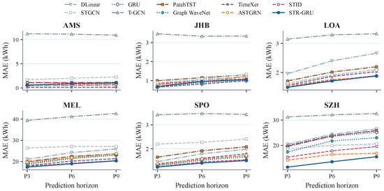
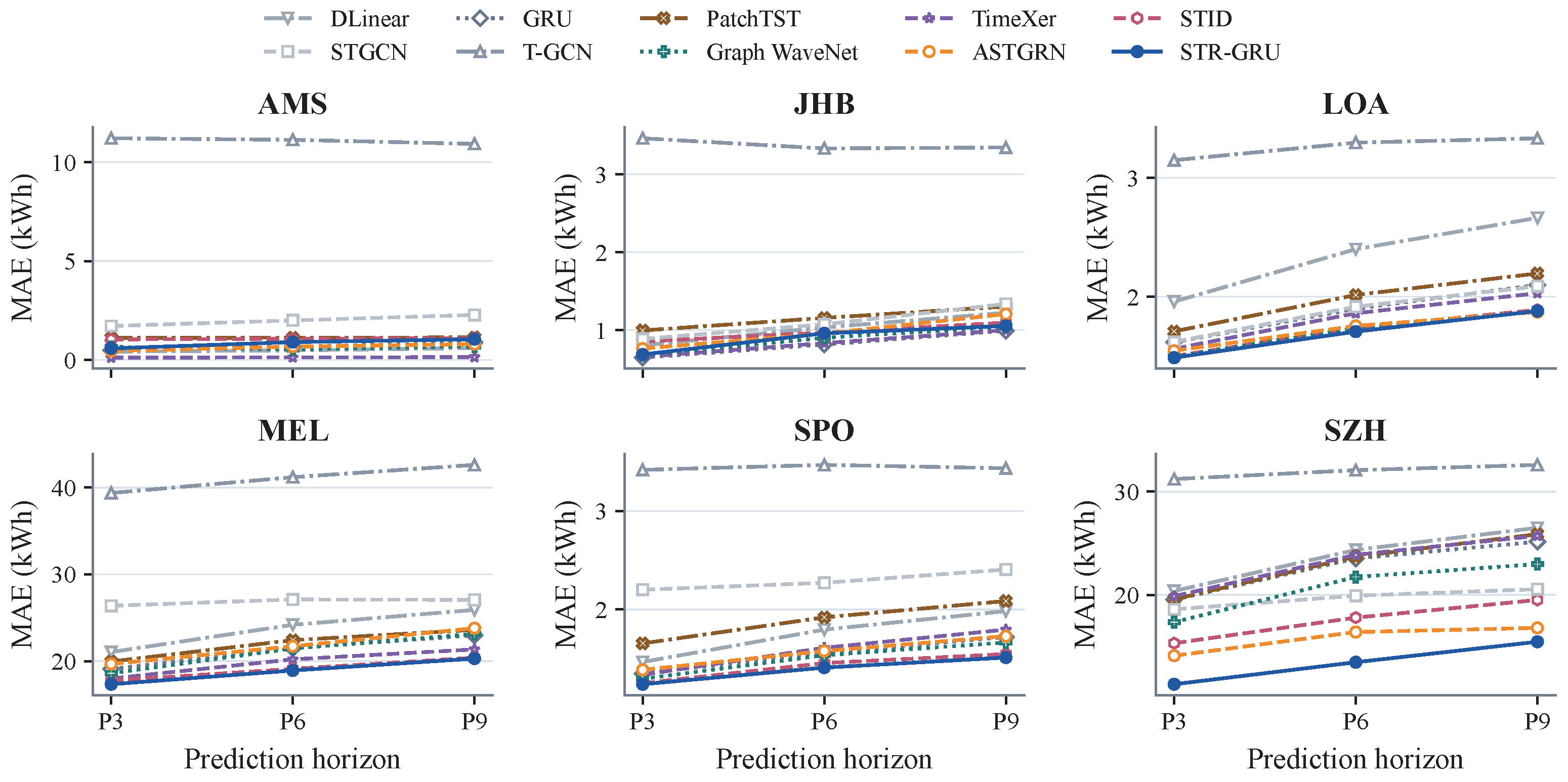
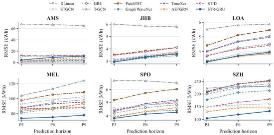
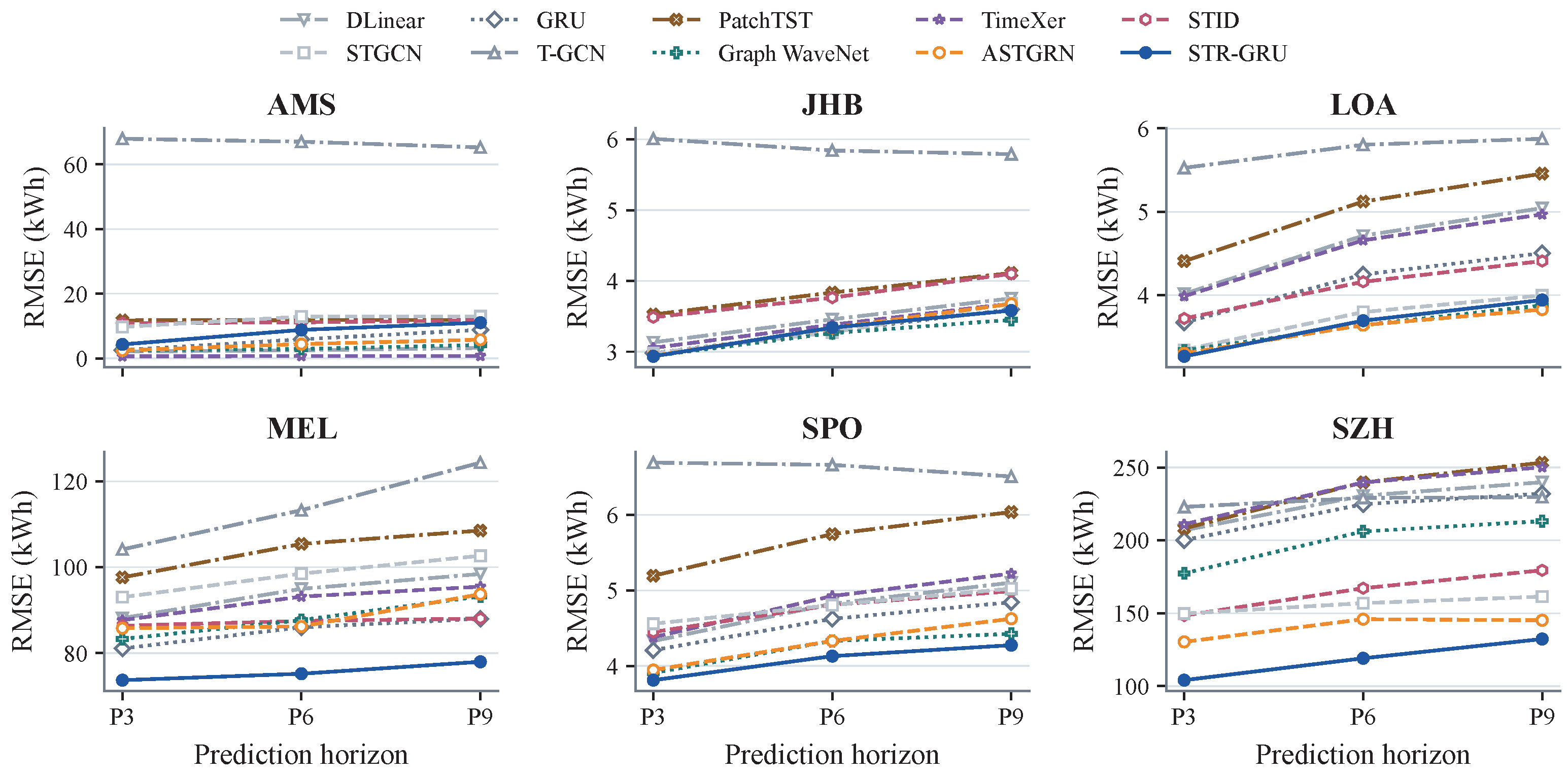
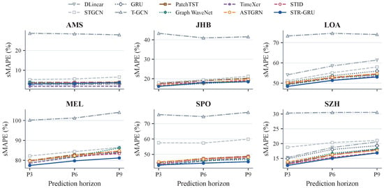
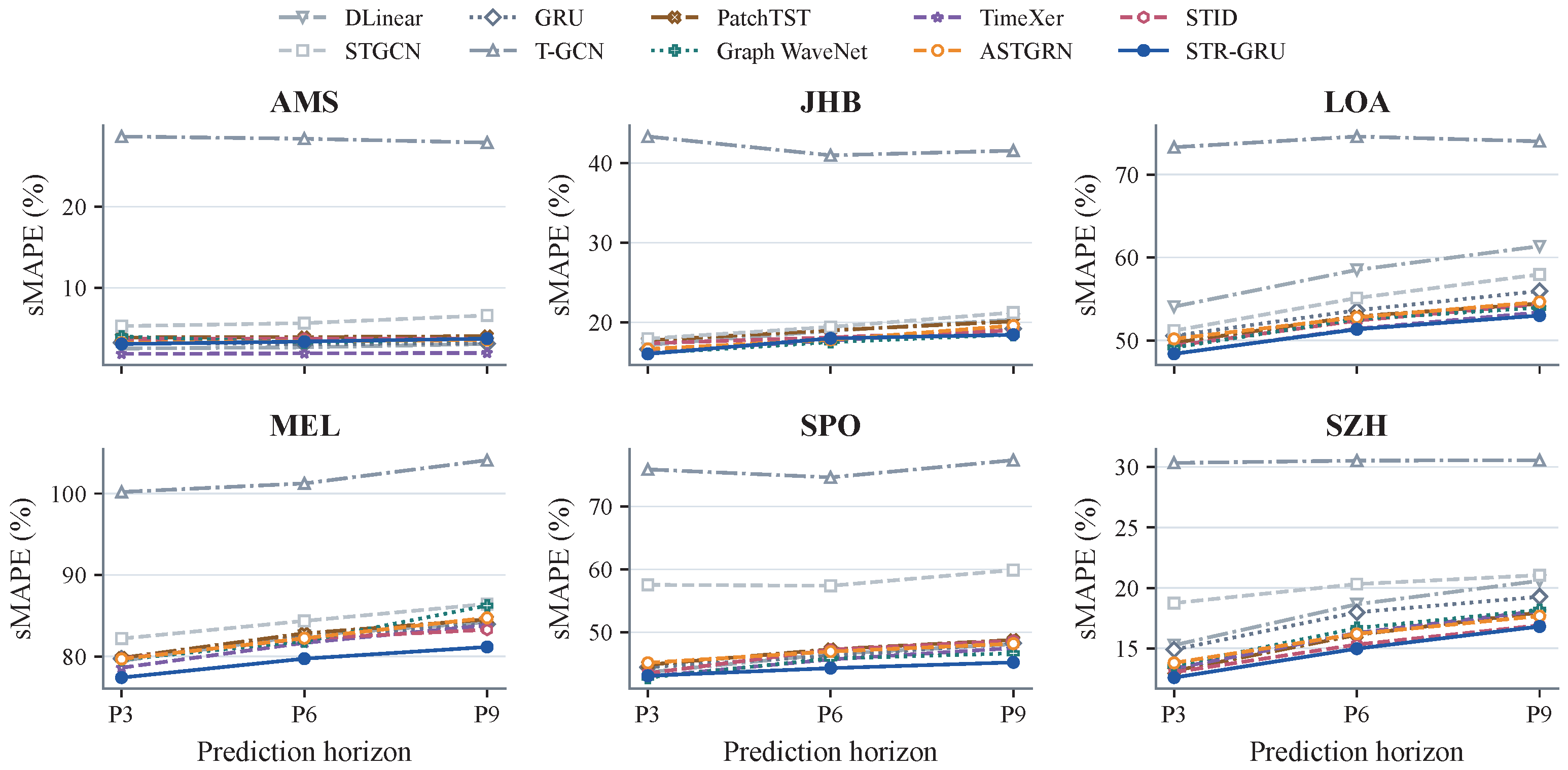
Figure 3, Figure 4 and Figure 5 compare MAE, RMSE, and sMAPE across P3, P6, and P9. Each metric is calculated using all predicted steps within the corresponding direct multi-step forecasting task.

Figure 3. MAE at different prediction horizons.

Figure 4. RMSE across prediction horizons.

Figure 5. sMAPE across prediction horizons.

STR-GRU achieves the lowest MAE and RMSE at all three forecasting horizons on MEL, SPO, and SZH. The improvements are largest on SZH, where MAE is 19.54%, 17.77%, and 7.98% lower than that of ASTGRN at P3, P6, and P9, respectively. The corresponding RMSE reductions are 20.16%, 18.38%, and 8.85%. Although the improvement becomes smaller as the forecasting horizon increases, STR-GRU maintains the lowest MAE and RMSE through P9.

The results on MEL and SPO show a similar pattern. At P6, STR-GRU reduces RMSE by 12.59% relative to GRU on MEL. On SPO, it reduces MAE by 3.15% relative to STID and RMSE by 4.65% relative to ASTGRN. STR-GRU also achieves the lowest sMAPE at every horizon on MEL and SZH and at P6 and P9 on SPO. On LOA, the results vary across horizons: STR-GRU has the lowest MAE at P3 and P6, while ASTGRN performs better at P9. These results show that the MAE and RMSE advantages of STR-GRU on MEL, SPO, and SZH are maintained across the evaluated forecasting horizons.

4.2.3. Station-Level Forecasting Analysis

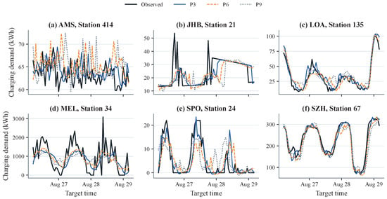
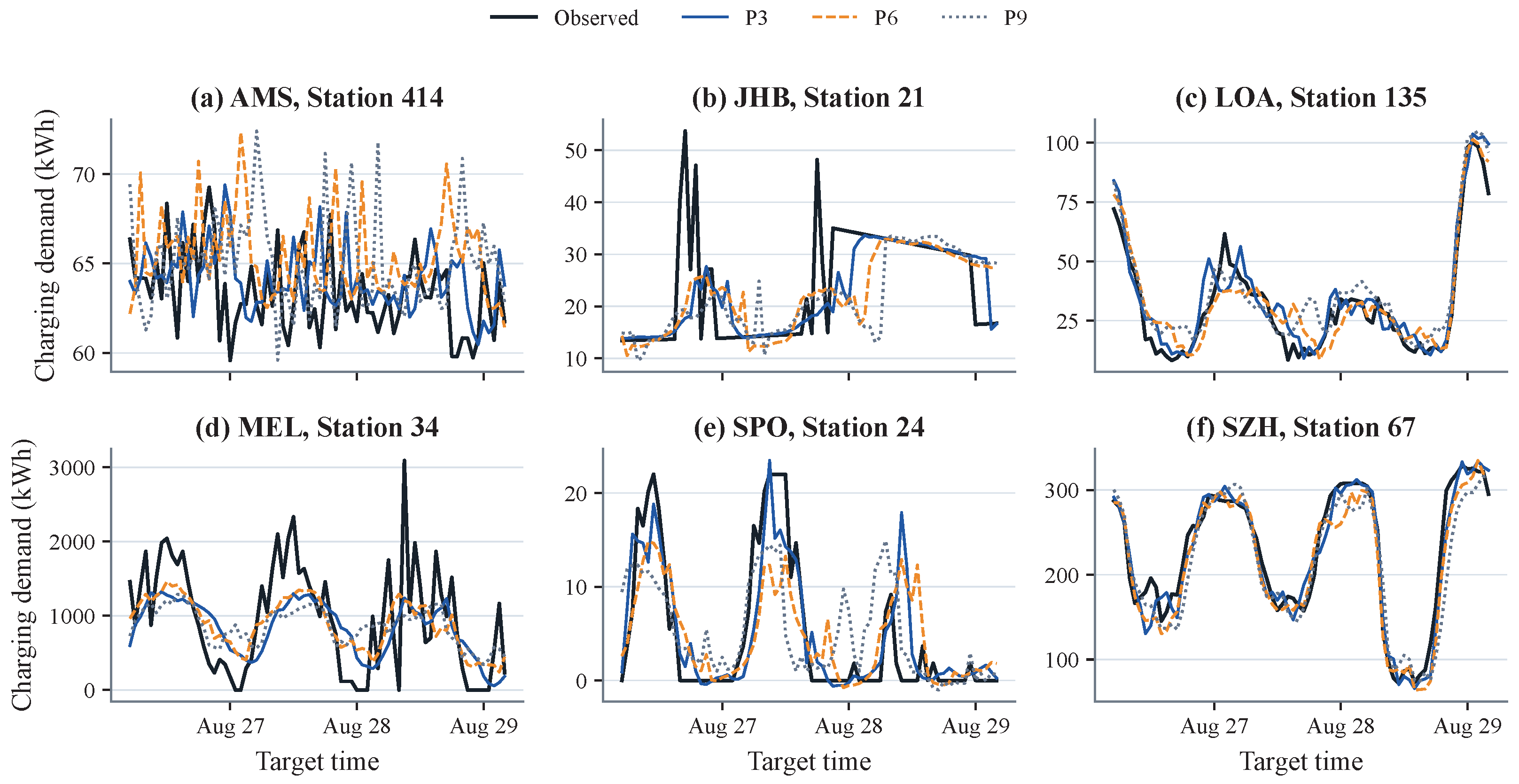
To further examine station-level forecasting behavior, Figure 6 presents illustrative forecasts from the six cities over a common 72-h period. For P3, P6, and P9, the final output step of each forecasting task is aligned with the corresponding observed demand.

Figure 6. Station-level demand forecasts.

Across the selected stations, the forecasts generally capture the main demand patterns despite clear differences in demand scale and variability. For AMS Station 414, the forecasts remain near the overall demand level, although many local peaks and troughs are not fully captured. Similar behavior is observed for LOA Station 135 and SZH Station 67, where the broad rises, declines, and low-demand intervals are captured. On SPO Station 24, the forecasts also capture the main recurring demand bursts and intervening low-demand periods, although differences remain in peak magnitudes and local fluctuations.

Abrupt local peaks are more difficult to predict. The observed peak of 53.712 kWh at JHB Station 21 is underestimated at all three forecasting horizons, and a similar underestimation occurs for the large demand peak at MEL Station 34. These examples show that STR-GRU can capture the main demand patterns in the selected stations, while abrupt peak magnitudes remain more difficult to predict. The peak-demand performance is examined quantitatively in the following section.

4.3. Daily Peak-Demand Evaluation

Daily peak demand is evaluated across all six cities using the same STR-GRU configurations and random seeds as in the main experiments. For each city, STR-GRU is compared with the non-STR-GRU model having the lowest horizon-averaged MAE in Table 3. Final-step predictions are aligned with their target timestamps, and the peak metrics are calculated using complete 24-h station-days. The same eligible station-days are used for STR-GRU and the selected baseline.

Following the daily peak-deviation measure for EV charging loads [39], Peak MAE is defined as

$$\mathrm{PeakMAE}={\displaystyle \frac{1}{K}}{\displaystyle \sum _{i=1}^K}\left|p_i-{\widehat{p}}_i\right|,$$

(30)

where $p_i={\max }_{h=0,\dots ,23}{y}_{i,h}$ and ${\widehat{p}}_i={\max }_{h=0,\dots ,23}{\widehat{y}}_{i,h}$ are the observed and predicted daily peak magnitudes of hourly charging energy (kWh), respectively, and K is the number of evaluated station-days.

Signed Peak Bias is defined as

$$\mathrm{PeakBias}=100\%{\displaystyle \frac{{\sum }_{i=1}^K({\widehat{p}}_i-p_i)}{{\sum }_{i=1}^K{p}_i}},$$

(31)

where negative values indicate overall underestimation and positive values indicate overall overestimation. Table 4 reports the mean and sample standard deviation across three seeds after averaging each metric over P3, P6, and P9 within each city and seed. Peak MAE measures the absolute error in daily peak magnitude, while signed Peak Bias measures the overall direction of peak-estimation error.

Table 4. Daily peak-demand errors.

City	Baseline	Peak MAE (kWh)		Peak Bias (%)
		STR-GRU	Baseline	STR-GRU	Baseline
AMS	TimeXer	$1.196\pm 0.155$	$0.339\pm 0.001$	$0.22\pm 0.67$	$-0.81\pm 0.01$
JHB	GRU	$2.413\pm 0.028$	$2.326\pm 0.043$	$-13.15\pm 0.37$	$-14.18\pm 0.14$
LOA	Graph WaveNet	$3.556\pm 0.071$	$3.246\pm 0.035$	$-4.00\pm 0.91$	$-16.60\pm 1.13$
MEL	STID	$34.510\pm 1.545$	$30.503\pm 0.852$	$-29.80\pm 1.72$	$-27.33\pm 1.17$
SPO	STID	$2.719\pm 0.028$	$2.685\pm 0.043$	$-25.82\pm 0.50$	$-27.69\pm 0.61$
SZH	ASTGRN	$14.406\pm 0.448$	$17.435\pm 1.529$	$-1.47\pm 0.47$	$-2.30\pm 1.21$

STR-GRU achieves a lower mean Peak MAE on SZH, decreasing from 17.435 kWh for ASTGRN to 14.406 kWh, corresponding to a 17.37% reduction. The selected baselines achieve lower Peak MAE in the other five cities, although the differences on JHB and SPO are small, at approximately 0.09 and 0.03 kWh, respectively. Thus, the improvement in absolute peak error is mainly observed on SZH.

The signed Peak Bias shows a different pattern. STR-GRU has bias closer to zero than the selected baselines on AMS, JHB, LOA, SPO, and SZH. On LOA, the bias changes from $-16.60\%$ to $-4.00\%$, a difference of 12.6 percentage points. The bias remains negative on JHB, MEL, SPO, LOA, and SZH, while AMS shows near-zero overall bias ($0.22\%$). These results show that STR-GRU reduces the overall peak-estimation bias in most of the evaluated cities.

The two metrics describe different aspects of peak-demand forecasting. STR-GRU reduces both Peak MAE and the magnitude of signed Peak Bias on SZH. On AMS, JHB, LOA, and SPO, its signed Peak Bias is closer to zero, while its Peak MAE is higher than that of the selected baseline. This difference occurs because positive and negative peak errors can offset each other in signed Peak Bias, whereas Peak MAE measures their absolute magnitudes. The two metrics therefore provide complementary information on daily peak forecasting.

4.4. Ablation Study

The ablation study evaluates the main modules and design choices of STR-GRU. We first examine LD-GRU, STRE, and the exogenous pathway, and then analyze the individual embeddings, STRE representation, and exogenous fusion strategies. Unless a forecasting horizon is specified, the reported averages are calculated over P3, P6, and P9 within the same city and metric. Relative reductions are calculated from these averages.

4.4.1. Core-Module Ablation

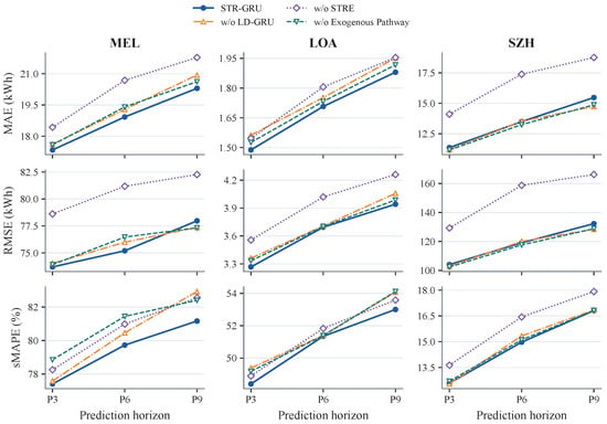
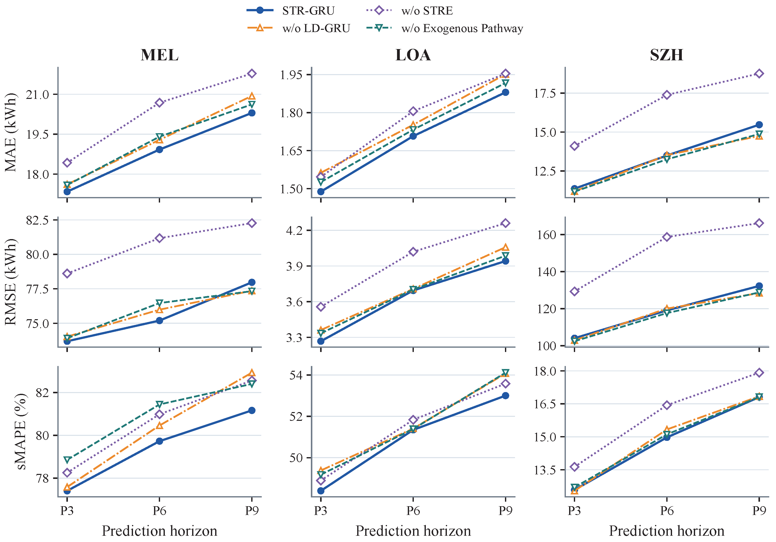
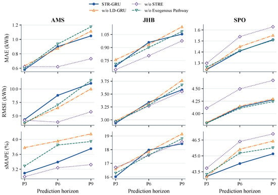
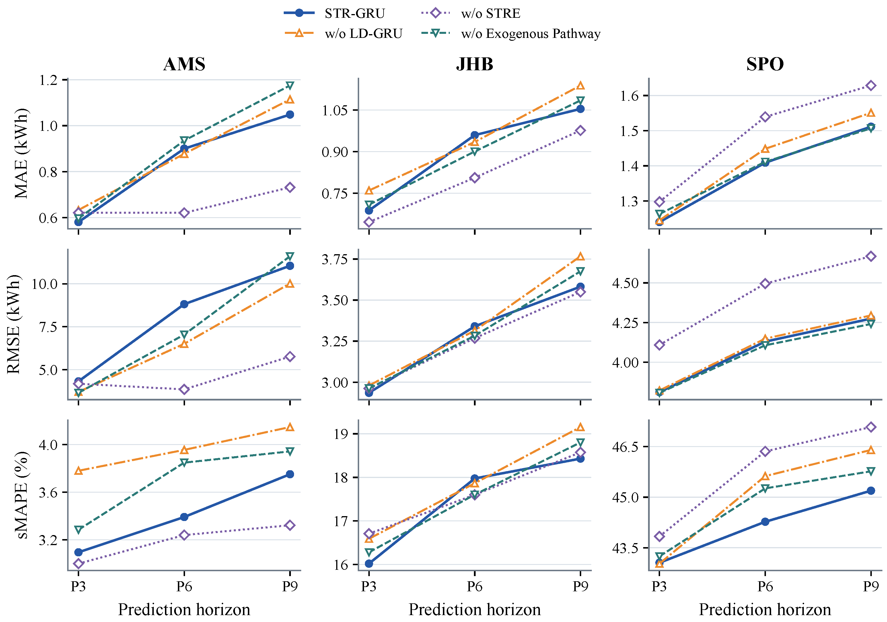
Figure 7 and Figure 8 compare STR-GRU with three variants. w/o LD-GRU replaces the level–difference dual-branch encoder with a single GRU. w/o STRE removes the spatio-temporal representation-enhancement module. w/o Exogenous Pathway removes electricity price and temperature together with their fusion pathway.

Figure 7. Core-module ablation on MEL, LOA, and SZH.

Figure 8. Core-module ablation on AMS, JHB, and SPO.

Compared with w/o LD-GRU, STR-GRU achieves lower horizon-averaged MAE, RMSE, and sMAPE on JHB, LOA, MEL, and SPO. MAE decreases by 4.65% on JHB and 3.62% on LOA. On LOA and SPO, both MAE and RMSE are lower at every forecasting horizon. Horizon-averaged sMAPE also decreases in all six cities, with reductions of 0.78–13.85%. Separately encoding demand levels and first-order differences allows the model to represent both overall demand evolution and recent short-term changes. The improvement is most consistent for sMAPE, together with absolute-error gains on JHB, LOA, MEL, and SPO.

STRE also improves performance on several charging networks. STR-GRU achieves lower horizon-averaged MAE, RMSE, and sMAPE than w/o STRE on MEL, LOA, SPO, and SZH. On SZH, MAE decreases from 16.752 to 13.445 kWh, while MAE, RMSE, and sMAPE are reduced by 19.74%, 21.75%, and 7.55%, respectively. The MAE reductions on MEL and SPO are 7.11% and 6.84%. These gains suggest that station-specific and recurring temporal information provides useful context beyond historical demand alone. In contrast, removing STRE gives lower values for all three metrics on AMS and lower MAE and RMSE on JHB, showing that its effect varies across charging networks.

The exogenous pathway also has different effects across networks. STR-GRU achieves lower horizon-averaged MAE, RMSE, and sMAPE than w/o Exogenous Pathway on LOA and MEL, while removing the pathway gives lower MAE and RMSE on SZH. This suggests that electricity price and temperature do not provide the same forecasting benefit in every charging network. Section 4.4.4 further examines the effect of exogenous inputs and their fusion strategy.

4.4.2. Embedding Ablation

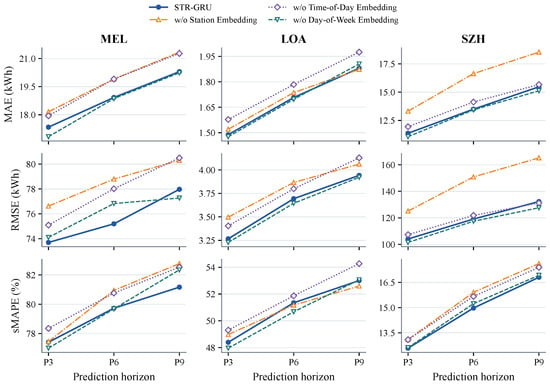
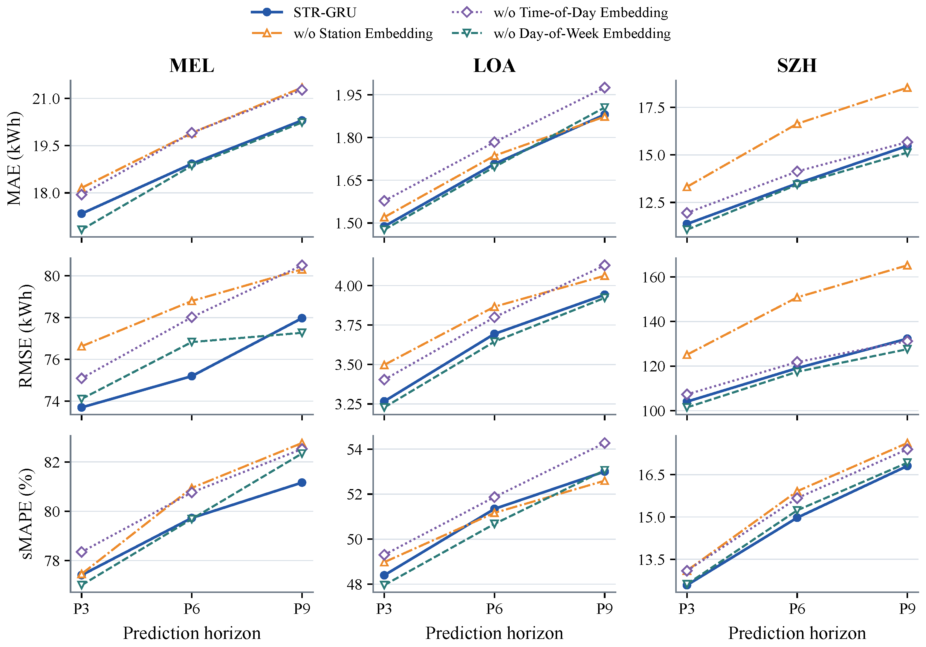
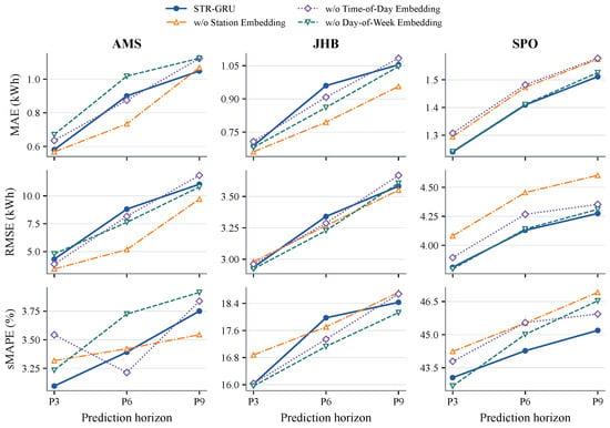
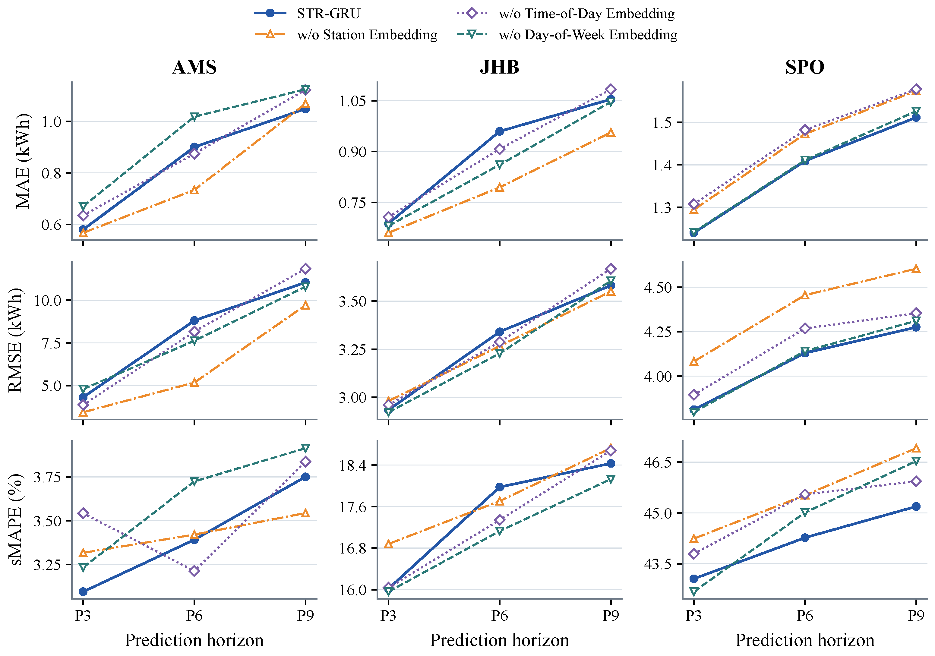
Figure 9 and Figure 10 compare variants that remove the station, time-of-day, and day-of-week embeddings separately while keeping the remaining architecture unchanged.

Figure 9. Embedding ablation on MEL, LOA, and SZH.

Figure 10. Embedding ablation on AMS, JHB, and SPO.

The station embedding provides clear gains on MEL, SPO, and SZH. Retaining this embedding lowers the horizon-averaged MAE, RMSE, and sMAPE on all three networks. On SZH, STR-GRU reduces these metrics by 16.83%, 19.43%, and 4.86%, respectively, compared with the variant without the station embedding. On SPO, MAE and RMSE decrease by 4.16% and 7.04%, while both metrics are lower at every horizon on MEL and SPO. This suggests that station identity provides useful information for distinguishing station-specific demand patterns. The effects on AMS and JHB vary by metric.

The time-of-day embedding also improves performance on several networks. Retaining this embedding lowers all three horizon-averaged errors on MEL, LOA, SPO, and SZH, with MAE reductions of 3.39–4.88% and RMSE reductions of 1.37–3.78%. This is consistent with the recurring intraday patterns in charging demand and supports the use of time-of-day information in addition to the 12-h demand history. The effect is not consistent at every horizon: on SZH, P9 RMSE is 132.294 kWh for STR-GRU and 131.205 kWh without the time-of-day embedding. The results on AMS and JHB also vary by metric.

The day-of-week embedding provides less consistent gains across cities and metrics. On MEL, SPO, and SZH, the horizon-averaged MAE benefit from the station or time-of-day embedding is larger than that from the day-of-week embedding. Among the three embeddings, station identity and time-of-day information therefore provide the most consistent gains on these networks.

4.4.3. STRE Representation Analysis

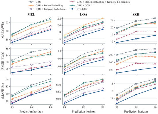
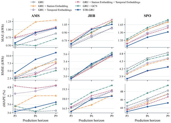
Figure 11 and Figure 12 compare GRU, GRU + Station Embedding, GRU + Temporal Embeddings, GRU + Station Embedding + Temporal Embeddings, and GRU + GCN. Temporal Embeddings include the time-of-day and day-of-week embeddings, while GRU + GCN uses distance-based graph convolution. The complete STR-GRU is included as an additional reference.

Figure 11. Representation comparison on MEL, LOA, and SZH.

Figure 12. Representation comparison on AMS, JHB, and SPO.

Combining station and temporal embeddings improves the basic GRU on several networks. GRU + Station Embedding + Temporal Embeddings achieves lower horizon-averaged MAE, RMSE, and sMAPE than GRU on MEL, SPO, and SZH. On SZH, the reductions reach 29.46%, 35.45%, and 8.09%, respectively. These results show that station and temporal identities provide useful information beyond historical demand alone.

The comparison with GRU + GCN further examines the spatial representation. Combined station and temporal embeddings achieve lower horizon-averaged MAE, RMSE, and sMAPE on MEL, LOA, SPO, and SZH. On SZH, MAE and RMSE decrease by 21.69% and 27.83%, respectively, while the reductions on MEL are 10.17% and 7.93%. These results suggest that station identities can provide useful spatial information without distance-based inter-station propagation on these networks. GRU + GCN performs better on all three metrics on AMS, while the results on JHB vary by metric. The relative benefit of identity-based and graph-based representations therefore depends on the charging network.

The complete STR-GRU provides further gains beyond the combined embeddings. Compared with GRU + Station Embedding + Temporal Embeddings, STR-GRU achieves lower horizon-averaged MAE in all six cities, including reductions of 9.01% on LOA and 16.19% on SZH. Its sMAPE is also lower in every city, while the RMSE ranking varies across cities. The complete STR-GRU therefore provides further gains beyond the combined embedding variant.

4.4.4. Exogenous Feature Fusion

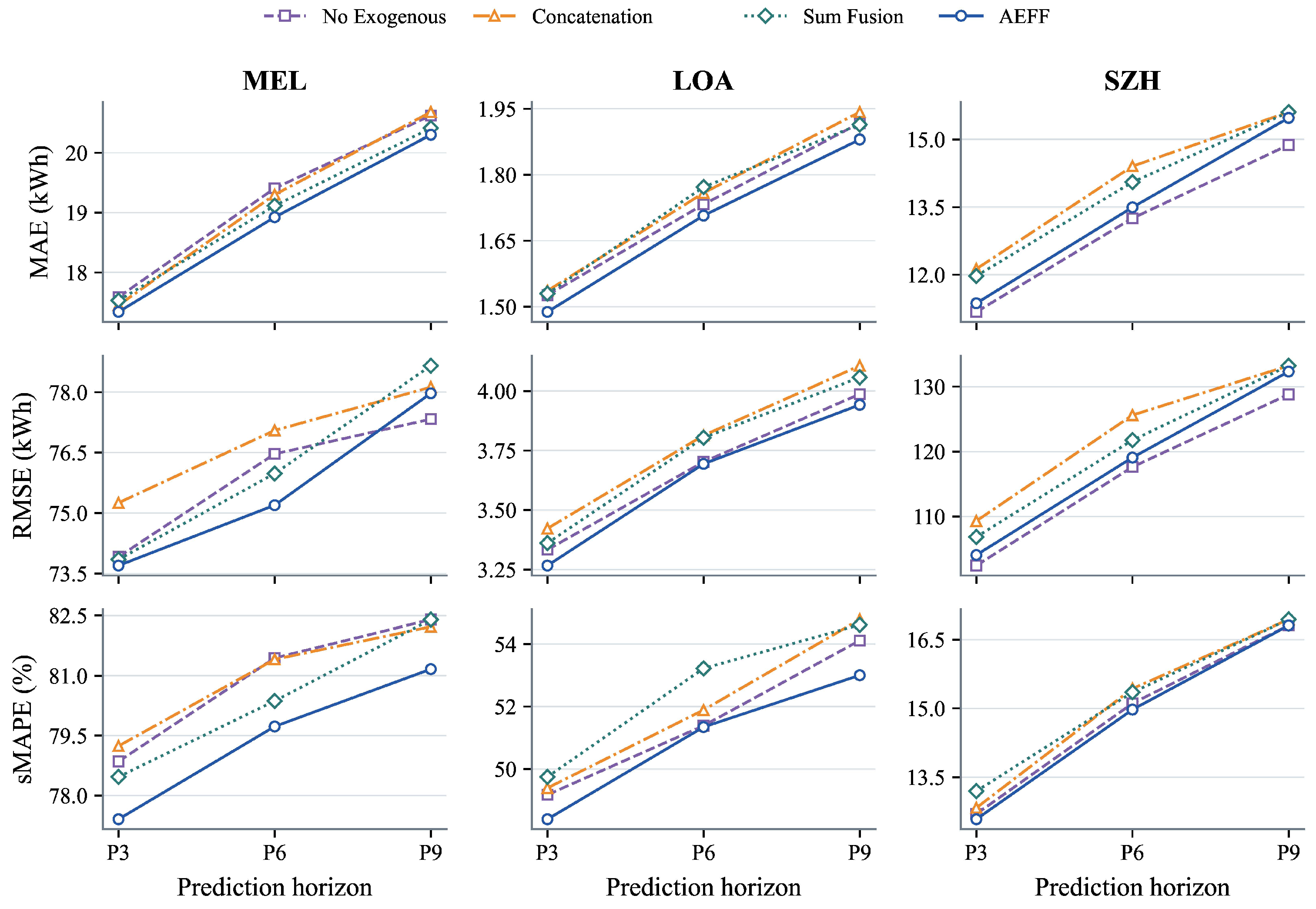
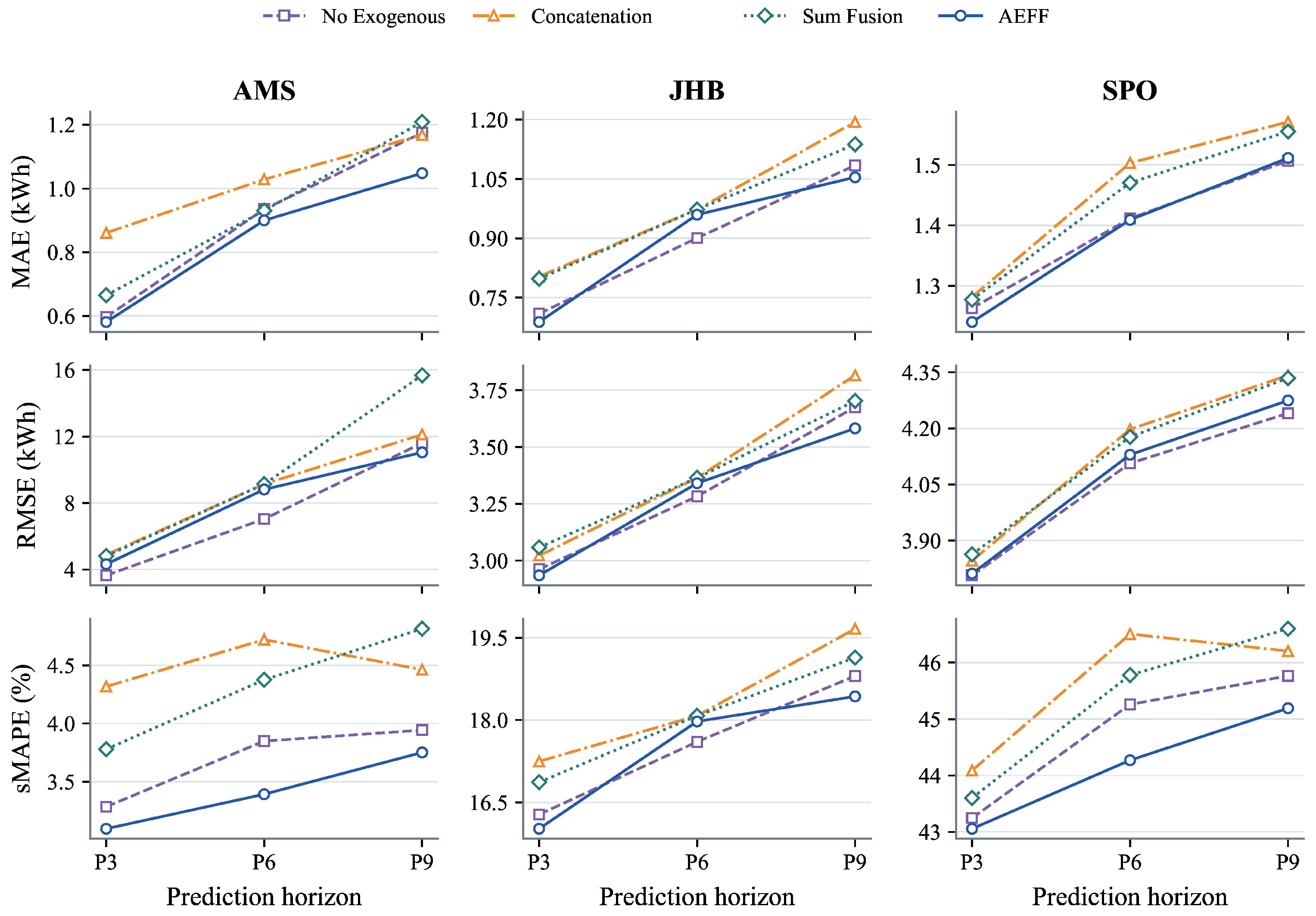
Figure 13 and Figure 14 compare four exogenous-feature configurations: No Exogenous, Concatenation, Sum Fusion, and AEFF. No Exogenous removes electricity price and temperature. Concatenation directly combines their encoded representations with the demand representation. Sum Fusion combines the encoded electricity price and temperature representations by element-wise addition, while AEFF generates station-conditioned fusion weights.

Figure 13. Exogenous fusion on MEL, LOA, and SZH.

Figure 14. Exogenous fusion on AMS, JHB, and SPO.

Following the aggregation used in Table 3, the comparisons below use the arithmetic mean of P3, P6, and P9 separately within each city and metric. The plotted curves retain the horizon-specific results, while the overall conclusions are based on these horizon averages.

Among the four configurations, AEFF achieves the lowest horizon-averaged MAE, RMSE, and sMAPE on MEL and LOA. On AMS and SPO, it has the lowest average MAE and sMAPE, while No Exogenous has lower average RMSE. On JHB, AEFF has the lowest average RMSE and sMAPE, whereas No Exogenous has lower average MAE. On SZH, AEFF has the lowest average sMAPE, while No Exogenous has lower average MAE and RMSE. Thus, the best configuration depends on the city and error metric even after averaging over the three forecasting horizons.

Restricting the comparison to the three configurations that include the same electricity-price and temperature inputs, AEFF has lower horizon-averaged MAE, RMSE, and sMAPE than Concatenation and Sum Fusion in all six cities. On AMS, its average MAE is 17.29% lower than Concatenation and 9.82% lower than Sum Fusion; the corresponding reductions on SZH are 4.27% and 3.11%. These average-error comparisons favor AEFF among the tested fusion designs, while the comparison with No Exogenous shows that the benefit of including external inputs remains city- and metric-dependent. The horizon-specific curves provide additional context for these average results. All comparisons describe reported means rather than statistical significance.

4.5. AEFF Fusion-Weight Analysis

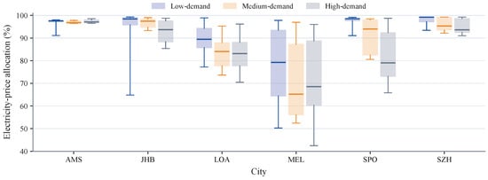
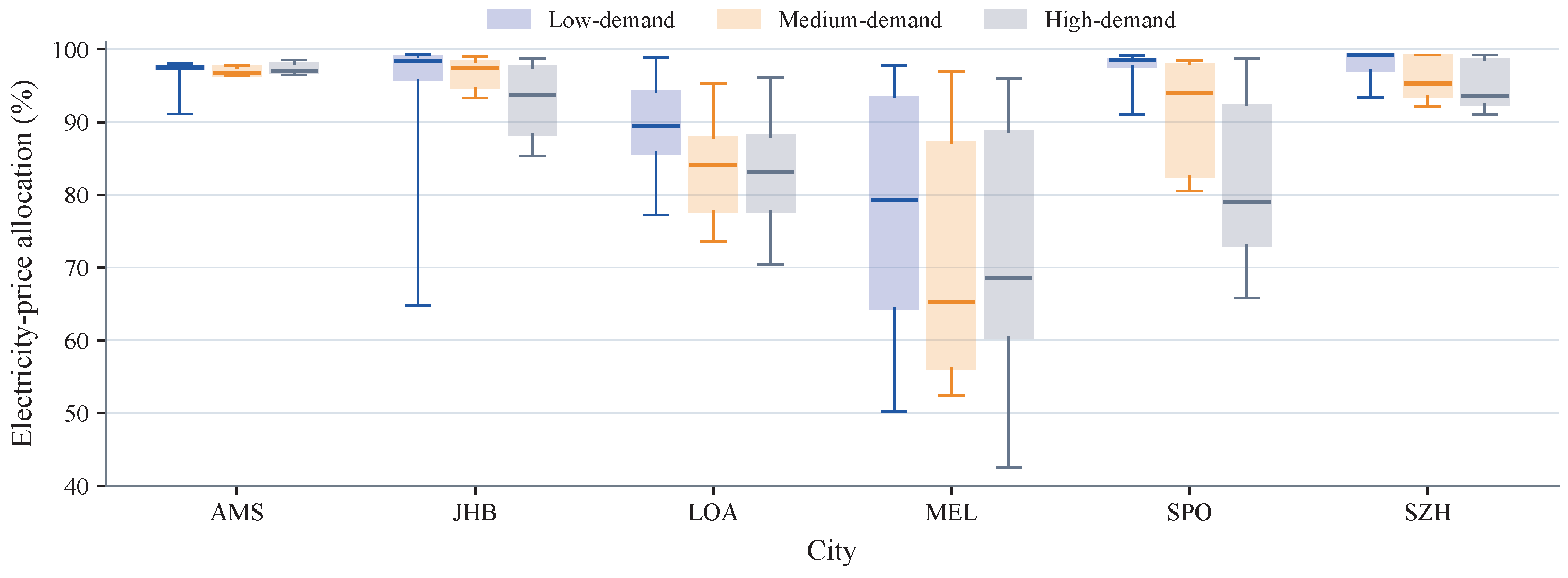
To examine the fusion behavior of AEFF, Figure 15 shows the learned weights for electricity price at P6. Within each city, stations are divided into three groups according to tertiles of mean training-set demand. Since the price and temperature weights sum to one, only the price weights are shown. Each box summarizes the station-level mean weights. The box spans the interquartile range, the internal line shows the median, and the whiskers extend to observations within the 5th–95th percentile range.

Figure 15. Electricity-price fusion weights by demand group.

The learned weights vary across cities and demand groups. AMS has high and concentrated weights for electricity price, with group medians ranging from 96.79% to 97.55%. MEL has lower and more dispersed weights, with medians of 79.23%, 65.25%, and 68.53% for the low-, medium-, and high-demand groups, respectively. On SPO, the median decreases from 98.53% in the low-demand group to 79.04% in the high-demand group, a difference of 19.49 percentage points. The median also decreases across demand groups on LOA and JHB, while SZH maintains high price weights. The relation between demand group and price weight therefore differs across cities, with no common trend across all six networks.

These distributions describe model-dependent allocations between the encoded electricity-price and temperature representations across stations and demand groups. The weights alone do not establish feature importance or a predictive benefit from adaptive weighting. The error comparisons in Section 4.4.4 separately assess forecasting performance, including the settings where No Exogenous has lower error.

4.6. Parameter Sensitivity Analysis

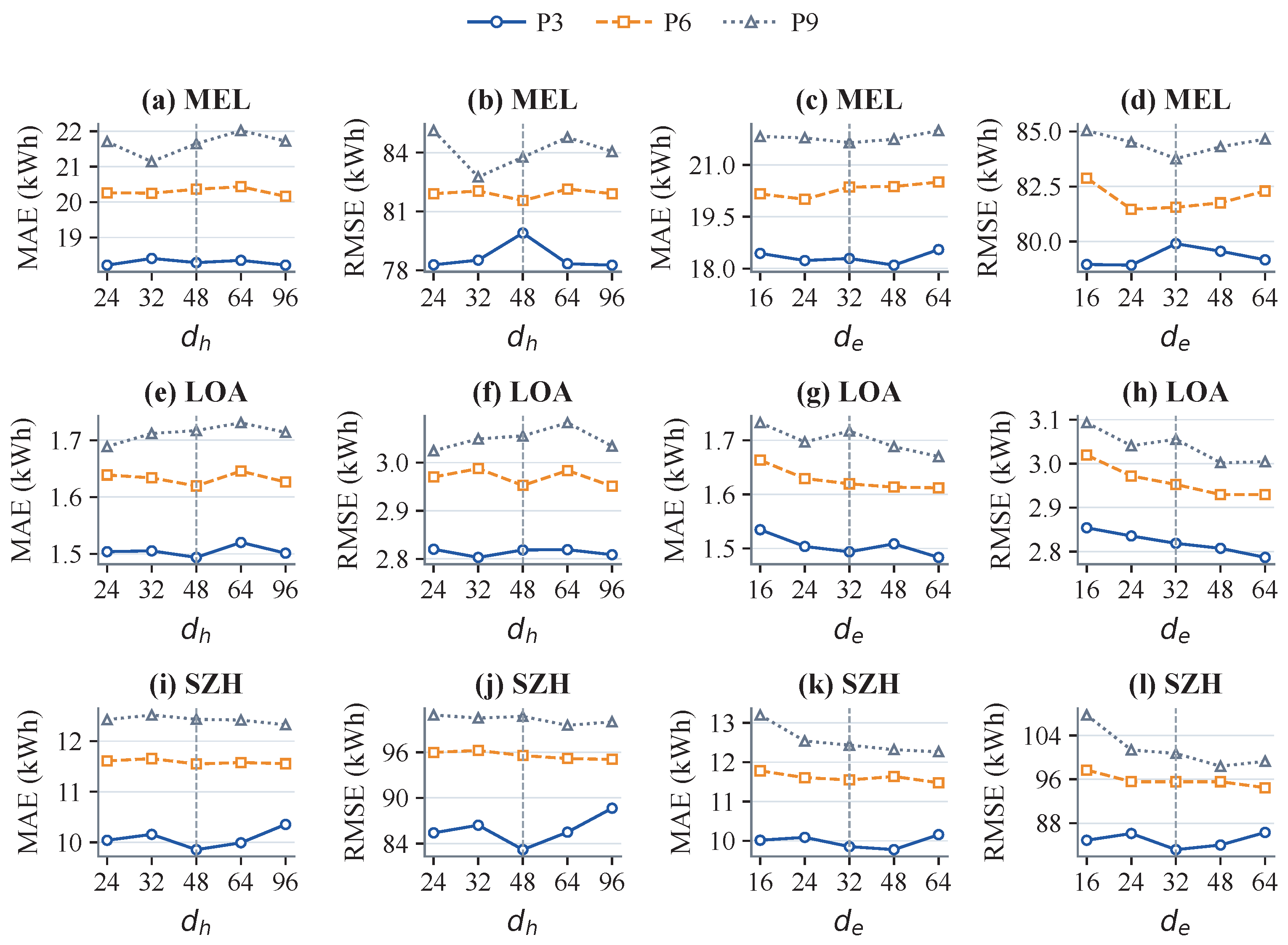
Parameter selection and sensitivity analysis are conducted in two stages. First, all 25 combinations of the temporal hidden dimension $d_h\in \{24, 32, 48, 64, 96\}$ and embedding dimension $d_e\in \{16, 24, 32, 48, 64\}$ are evaluated on the validation sets of the six cities. For each city and configuration, validation MAE is averaged over P3, P6, and P9. The resulting city-wise comparisons are used to select $(d_h,d_e)=(48, 32)$ as a common configuration for the main experiments.

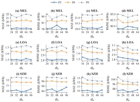
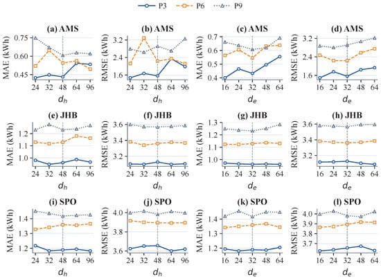
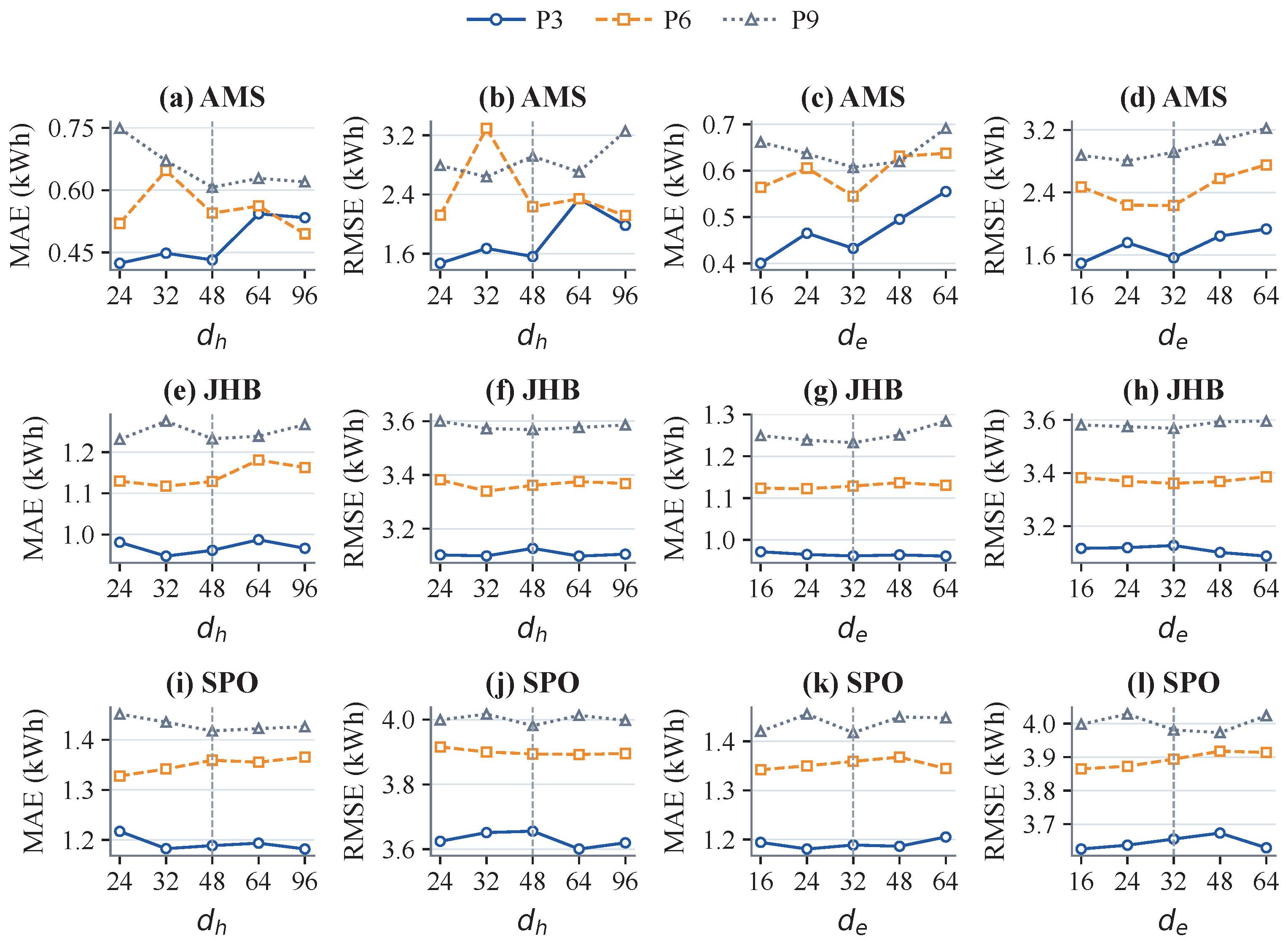
A one-factor-at-a-time analysis is then performed around this common configuration. The temporal hidden dimension is varied over $\{24, 32, 48, 64, 96\}$ with $d_e=32$ fixed, while the embedding dimension is varied over $\{16, 24, 32, 48, 64\}$ with $d_h=48$ fixed. Figure 16 and Figure 17 show the results for MEL, LOA, and SZH and for AMS, JHB, and SPO, respectively. The curves report validation MAE and RMSE on the original demand scale for P3, P6, and P9.

Figure 16. Parameter sensitivity on MEL, LOA, and SZH.

Figure 17. Parameter sensitivity on AMS, JHB, and SPO.

Increasing $d_h$ does not consistently reduce forecasting error. The lowest horizon-averaged MAE occurs at $d_h=48$ on AMS, JHB, LOA, and SZH and at $d_h=32$ on MEL and SPO. For example, horizon-averaged MAE on LOA varies only from 1.610 to 1.632 kWh across the examined hidden dimensions, while increasing $d_h$ from 48 to 96 on SZH slightly increases both MAE and RMSE. Thus, a larger hidden dimension does not necessarily lead to lower forecasting error.

The response to $d_e$ is more city dependent. The lowest horizon-averaged MAE occurs at $d_e=32$ on AMS and JHB, at $d_e=24$ on MEL, and at $d_e=16$ on SPO, while the corresponding minima occur at $d_e=64$ on LOA and $d_e=48$ on SZH. The preferred embedding dimension therefore varies across cities.

The one-factor results support the selected configuration. With $d_e=32$ fixed, $d_h=48$ achieves the lowest horizon-averaged validation MAE on AMS, JHB, LOA, and SZH and is only 0.83% and 0.15% above the respective minima on MEL and SPO. With $d_h=48$ fixed, $d_e=32$ is within 1.36% of the minimum in each city. These results support $d_h=48$ and $d_e=32$ as a common configuration across the six cities.

4.7. Computational Efficiency

Table 5 reports the parameter count, training time per epoch, and median inference latency for P6 using seed 2025 and FP32 precision on an NVIDIA GeForce RTX 5080 GPU. Training times use the reported model-specific configurations, while inference latency is measured with a batch size of one.

Table 5. Computational efficiency on P6.

Model/City (N)	AMS (1388)	JHB (35)	LOA (224)	MEL (62)	SPO (41)	SZH (1379)
(a) Parameters (K)
DLinear	0.2	0.2	0.2	0.2	0.2	0.2
GRU	13.3	13.3	13.3	13.3	13.3	13.3
PatchTST	403.5	403.5	403.5	403.5	403.5	403.5
TimeXer	665.0	665.0	665.0	665.0	665.0	665.0
STID	146.4	103.1	109.2	104.0	103.3	146.2
STGCN	1076.5	210.5	331.5	227.8	214.4	1070.7
T-GCN	13.1	13.1	13.1	13.1	13.1	13.1
Graph WaveNet	314.2	287.1	290.9	287.7	287.3	314.0
ASTGRN	266.0	252.5	254.4	252.8	252.5	265.9
STR-GRU (Ours)	134.2	112.6	115.6	113.0	112.7	134.1
(b) Training time (s/epoch)
DLinear	0.111	0.152	0.106	0.158	0.111	0.110
GRU	1.330	0.090	0.206	0.073	0.073	1.320
PatchTST	13.575	0.432	2.249	0.575	0.439	13.417
TimeXer	23.349	0.792	4.197	1.042	0.812	23.906
STID	1.436	0.064	0.236	0.080	0.065	1.456
STGCN	3.097	0.147	0.289	0.147	0.153	3.116
T-GCN	4.515	0.599	0.608	0.600	0.590	4.570
Graph WaveNet	16.996	0.406	1.671	0.418	0.408	17.732
ASTGRN	9.884	1.507	1.478	1.481	1.479	9.932
STR-GRU (Ours)	2.722	0.687	0.721	0.688	0.674	2.699
(c) Median inference latency (ms/window)
DLinear	0.151	0.123	0.123	0.142	0.131	0.123
GRU	0.163	0.104	0.099	0.114	0.109	0.165
PatchTST	1.960	1.225	1.247	1.273	1.263	1.961
TimeXer	3.066	0.962	1.279	1.024	1.004	3.168
STID	0.214	0.204	0.229	0.218	0.202	0.213
STGCN	1.178	0.531	0.524	0.511	0.553	1.176
T-GCN	1.567	1.679	1.681	1.696	1.646	1.614
Graph WaveNet	3.060	2.518	2.431	2.500	2.419	3.252
ASTGRN	9.159	4.353	4.201	4.267	4.262	9.132
STR-GRU (Ours)	1.023	1.068	1.020	1.038	1.016	1.026

STR-GRU contains 112.6–134.2 K trainable parameters across the six charging networks. On AMS, its parameter count is 49.55% lower than that of ASTGRN and 79.82% lower than that of TimeXer, while PatchTST contains 403.5 K parameters. Thus, STR-GRU uses fewer parameters than several larger baselines.

The runtime differences are most clear on AMS and SZH. STR-GRU requires approximately 2.7 s per epoch, compared with approximately 9.9 s for ASTGRN and 23.3–23.9 s for TimeXer under the reported configurations. Its inference latency is approximately 1.02–1.03 ms and is lower than that of ASTGRN and PatchTST on these two networks. On AMS, training time per epoch is 72.46% lower than that of ASTGRN, while inference latency is 88.83% lower.

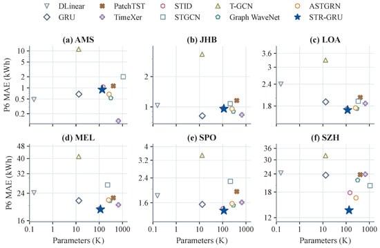
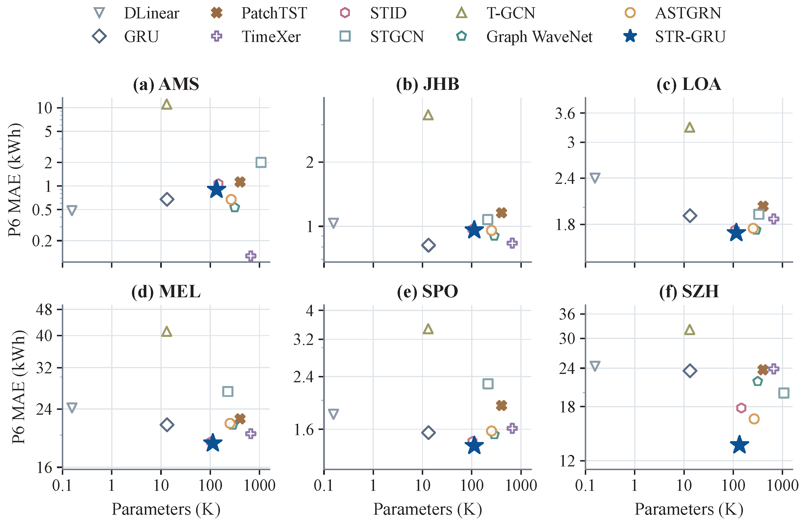
Figure 18 compares P6 MAE, averaged over the three random seeds, with trainable parameter count for each charging network. Both axes use logarithmic scales.

Figure 18. Accuracy–parameter trade-off.

On MEL, LOA, SPO, and SZH, STR-GRU achieves the lowest P6 MAE while using fewer parameters than PatchTST, TimeXer, STGCN, Graph WaveNet, and ASTGRN. TimeXer achieves the lowest P6 MAE on AMS, while GRU achieves the lowest on JHB.

On SZH, STR-GRU reduces P6 MAE by 17.77% relative to ASTGRN while using 49.58% fewer parameters. On MEL, it achieves the lowest P6 MAE with 113.0 K parameters, compared with 403.5 K for PatchTST and 665.0 K for TimeXer. Although DLinear, GRU, and T-GCN use fewer parameters, they have higher P6 MAE on MEL, LOA, SPO, and SZH. These results show a favorable balance between forecasting accuracy, model size, and measured runtime.

5. Discussion

Across the six charging networks, STR-GRU shows competitive forecasting performance, while its relative advantages vary across cities and forecasting settings. Results from the LD-GRU ablation help explain part of this variation. Separating historical demand levels from first-order differences provides useful additional information on several networks. Historical demand describes overall demand evolution, while first-order differences make recent changes more explicit. The varying gains suggest that difference encoding is most useful when short-term variations contain predictive information that is not fully represented by the original demand sequence. Its contribution therefore depends on the demand characteristics of the target charging network.

Controlled representation experiments provide further insight into the role of STRE. Station embeddings represent demand differences across spatially distinct stations, while time-of-day and day-of-week embeddings represent recurring intraday and weekly patterns. This design is related to the identity-based representation used in STID [31]. In STR-GRU, these representations are integrated with level–difference temporal encoding to form the enhanced demand representation, which is subsequently used in exogenous feature fusion. Compared with the basic GRU, the combined station and temporal embeddings reduce the three horizon-averaged errors on MEL, SPO, and SZH. Compared with the tested distance-based graph convolution, they perform better on MEL, LOA, SPO, and SZH, whereas GRU + GCN performs better on AMS and gives mixed results on JHB. Geographic distance may not always reflect charging-demand relationships between stations [14]. These results suggest that identity-based representation and graph-based modeling capture different aspects of station-level charging demand. Representation-based modeling is particularly useful when station-specific demand differences and recurring temporal patterns provide strong predictive information, while graph-based modeling can remain effective when inter-station relationships provide additional information.

Exogenous-feature experiments reveal a similar dependence on the charging network. Electricity price and temperature provide useful predictive information in some settings, while their contribution is smaller or mixed in others. The comparison with No Exogenous reflects the value of introducing these variables, whereas the fusion comparisons examine how the same exogenous information is integrated. AEFF achieves lower errors than the simpler fusion methods in several settings, while Concatenation or Sum Fusion remains competitive in others. This distinction shows that the value of exogenous inputs and the value of a particular fusion strategy are related but separate issues. Learned fusion weights also vary across cities and station demand groups. High price weights in several settings indicate that AEFF allocates a larger share of the encoded exogenous information to electricity price, while the variation across stations and cities shows that this allocation changes with the demand context. Overall, the results suggest that both exogenous information and its fusion strategy should be considered in relation to the target charging network and forecasting task.

City-level rankings further illustrate how model design interacts with network characteristics. TimeXer performs particularly well on AMS. Its explicit modeling of interactions between endogenous and exogenous time series may be well suited to the demand characteristics of this network. Results on JHB are more mixed: GRU gives the lowest MAE, while Graph WaveNet gives the lowest RMSE and sMAPE. This indicates that temporal modeling and inter-station modeling provide different benefits on this smaller network. SZH presents a different demand pattern, with a strongly right-skewed distribution and much larger values in its upper tail. Station-wise standardization reduces scale differences during training, while inverse transformation restores the original kWh scale for evaluation. Large-demand observations therefore have a greater effect on absolute errors, particularly RMSE. The clear STRE gains on SZH further indicate that station and temporal representations are useful under this demand pattern. Taken together, these city-level differences show that forecasting performance depends on the interaction between model design and the characteristics of the target charging network.

Computational results provide an additional perspective on model selection. Increasing the hidden or embedding dimension does not consistently reduce validation error, and the selected configuration remains close to the city-specific minima without using the largest tested dimensions. STR-GRU also uses fewer parameters than several graph- and Transformer-based baselines and has competitive measured runtime under the reported settings. DLinear and GRU use fewer parameters, while STID can be faster. On the larger AMS and SZH networks, STR-GRU remains compact and efficient compared with several more complex baselines while maintaining competitive forecasting performance. These results indicate that the main computational advantage of STR-GRU lies in its favorable balance between forecasting accuracy and model cost. This balance is particularly relevant for station-level forecasting on larger charging networks.

Peak-demand evaluation provides a complementary view of forecasting performance. STR-GRU reproduces recurring demand patterns in the selected station-level examples, while abrupt peaks remain more difficult to predict. It achieves lower horizon-averaged Peak MAE on SZH, whereas the selected baselines have lower Peak MAE in the other five cities. Peak Bias is closer to zero for STR-GRU on AMS, JHB, LOA, SPO, and SZH, but not on MEL. Because positive and negative errors can cancel in signed Peak Bias, Peak MAE and Peak Bias describe different aspects of peak forecasting. These results show that peak-specific evaluation provides information beyond average MAE and RMSE and is important when forecasts are used for station operation and local grid management. Peak-aware objectives, peak-timing evaluation, and uncertainty estimation therefore provide useful directions for improving forecasting performance during high-demand periods.

Generalization to unseen stations and new cities is another important direction for future work. Station embeddings are learned from the station identities observed during training, so a new station requires an initial representation before the learned identity-based information can be used. Station attributes such as location, charging capacity, station type, and nearby points of interest could provide this initial representation, followed by adaptation using early demand observations. Cross-city transfer could also be explored using the multi-city dataset. Future work could further combine station embeddings with selected inter-station spatial relationships and include additional variables such as traffic conditions and calendar events. These extensions could improve the applicability of STR-GRU to unseen stations, new cities, and broader operating conditions.

6. Conclusions

This study proposed STR-GRU for short-term station-level EV charging demand forecasting. STR-GRU combines level–difference temporal modeling, spatio-temporal representation enhancement, and adaptive exogenous feature fusion. LD-GRU separately encodes historical demand levels and first-order differences to model overall demand evolution and short-term variations. STRE uses station, time-of-day, and day-of-week embeddings to represent demand differences across spatially distinct stations and recurring temporal patterns without inter-station graph construction or information propagation. AEFF adaptively fuses electricity price and temperature according to station-specific demand representations.

Experiments on six urban charging networks and three forecasting horizons show that STR-GRU achieves the lowest horizon-averaged MAE, RMSE, and sMAPE on MEL, SPO, and SZH and the lowest MAE and sMAPE on LOA. The ablation and controlled representation experiments show that the effects of level–difference temporal modeling and spatio-temporal representation vary across charging networks. Using the same P3/P6/P9 averaging as the main comparison, AEFF achieves the lowest average errors for all three metrics on MEL and LOA in the fusion experiment. It also has lower horizon-averaged errors than Concatenation and Sum Fusion in all six cities, while No Exogenous is better on several city–metric combinations. The overall value of exogenous inputs therefore remains city- and metric-dependent. The computational results show a favorable balance between forecasting accuracy, model size, and measured runtime. The peak-demand evaluation also shows that abrupt demand peaks remain difficult to predict. Overall, STR-GRU provides competitive forecasting performance and a favorable accuracy–efficiency trade-off on several evaluated charging networks, while its effectiveness depends on the characteristics of the target network.

These limitations motivate further work on abrupt-peak prediction and generalization to unseen stations and new charging networks. Attribute-based station representations and cross-city transfer will be studied to improve generalization beyond the stations used for training. Future work will also examine selective inter-station modeling and additional exogenous variables under broader forecasting settings.

References

- Sarda, J.; Patel, N.; Patel, H.; Vaghela, R.; Brahma, B.; Bhoi, A.K.; Barsocchi, P. A Review of the Electric Vehicle Charging Technology, Impact on Grid Integration, Policy Consequences, Challenges and Future Trends. Energy Rep. 2024, 12, 5671–5692. [Google Scholar] [CrossRef] [Scilit]
- Patil, P.; Kazemzadeh, K.; Bansal, P. Integration of Charging Behavior into Infrastructure Planning and Management of Electric Vehicles: A Systematic Review and Framework. Sustain. Cities Soc. 2023, 88, 104265. [Google Scholar] [CrossRef] [Scilit]
- Srivastava, A.; Manas, M.; Dubey, R.K. Integration of Power Systems with Electric Vehicles: A Comprehensive Review of Impact on Power Quality and Relevant Enhancements. Electr. Power Syst. Res. 2024, 234, 110572. [Google Scholar] [CrossRef] [Scilit]
- Rashid, M.; Elfouly, T.; Chen, N. A Comprehensive Survey of Electric Vehicle Charging Demand Forecasting Techniques. IEEE Open J. Veh. Technol. 2024, 5, 1348–1373. [Google Scholar] [CrossRef] [Scilit]
- Wang, S.; Chen, A.; Wang, P.; Zhuge, C. Predicting Electric Vehicle Charging Demand Using a Heterogeneous Spatio-Temporal Graph Convolutional Network. Transp. Res. Part C Emerg. Technol. 2023, 153, 104205. [Google Scholar] [CrossRef] [Scilit]
- Wang, S.; Zhuge, C.; Shao, C.; Wang, P.; Yang, X.; Wang, S. Short-Term Electric Vehicle Charging Demand Prediction: A Deep Learning Approach. Appl. Energy 2023, 340, 121032. [Google Scholar] [CrossRef] [Scilit]
- Kuang, H.; Qu, H.; Deng, K.; Li, J. A Physics-Informed Graph Learning Approach for Citywide Electric Vehicle Charging Demand Prediction and Pricing. Appl. Energy 2024, 363, 123059. [Google Scholar] [CrossRef] [Scilit]
- Kuang, H.; Deng, K.; You, L.; Li, J. Citywide Electric Vehicle Charging Demand Prediction Approach Considering Urban Region and Dynamic Influences. Energy 2025, 320, 135170. [Google Scholar] [CrossRef] [Scilit]
- Jiang, D.; Gong, X.; Wei, Y.; Peng, B.; Xu, Z. An Electric Vehicle Charging Demand Prediction Approach Based on a Graph-Based Spatio-Temporal Attention Network. Sustain. Energy Grids Netw. 2025, 44, 101975. [Google Scholar] [CrossRef] [Scilit]
- Ostermann, A.; Haug, T. Probabilistic Forecast of Electric Vehicle Charging Demand: Analysis of Different Aggregation Levels and Energy Procurement. Energy Inform. 2024, 7, 13. [Google Scholar] [CrossRef] [Scilit]
- Ma, T.Y.; Faye, S. Multistep Electric Vehicle Charging Station Occupancy Prediction Using Hybrid LSTM Neural Networks. Energy 2022, 244, 123217. [Google Scholar] [CrossRef] [Scilit]
- Shi, J.; Zhang, W.; Bao, Y.; Gao, D.W.; Wang, Z. Load Forecasting of Electric Vehicle Charging Stations: Attention Based Spatiotemporal Multi-Graph Convolutional Networks. IEEE Trans. Smart Grid 2024, 15, 3016–3027. [Google Scholar] [CrossRef] [Scilit]
- Kim, H.J.; Kim, M.K. Spatial-Temporal Graph Convolutional-Based Recurrent Network for Electric Vehicle Charging Stations Demand Forecasting in Energy Market. IEEE Trans. Smart Grid 2024, 15, 3979–3993. [Google Scholar] [CrossRef] [Scilit]
- Wang, S.; Li, Y.; Shao, C.; Wang, P.; Wang, A.; Zhuge, C. An Adaptive Spatio-Temporal Graph Recurrent Network for Short-Term Electric Vehicle Charging Demand Prediction. Appl. Energy 2025, 383, 125320. [Google Scholar] [CrossRef] [Scilit]
- Bao, Z.; Hu, Z.; Kammen, D.M.; Su, Y. Data-Driven Approach for Analyzing Spatiotemporal Price Elasticities of EV Public Charging Demands Based on Conditional Random Fields. IEEE Trans. Smart Grid 2021, 12, 4363–4376. [Google Scholar] [CrossRef] [Scilit]
- Kuang, H.; Zhang, X.; Qu, H.; You, L.; Zhu, R.; Li, J. Unraveling the Effect of Electricity Price on Electric Vehicle Charging Behavior: A Case Study in Shenzhen, China. Sustain. Cities Soc. 2024, 115, 105836. [Google Scholar] [CrossRef] [Scilit]
- Wang, W.; Tang, A.; Wei, F.; Yang, H.; Xinran, L.; Peng, J. Electric Vehicle Charging Load Forecasting Considering Weather Impact. Appl. Energy 2025, 383, 125337. [Google Scholar] [CrossRef] [Scilit]
- Cao, T.; Xu, Y.; Liu, G.; Tao, S.; Tang, W.; Sun, H. Feature-Enhanced Deep Learning Method for Electric Vehicle Charging Demand Probabilistic Forecasting of Charging Station. Appl. Energy 2024, 371, 123751. [Google Scholar] [CrossRef] [Scilit]
- Yang, M.; Li, W.; Sun, P.; Su, X.; Huang, T.; Zheng, T. Charging-Load Prediction for Electric Vehicle Stations Using Correlation Analysis and RIME-CNN-LSTM-Attention Model. IET Gener. Transm. Distrib. 2026, 20, e70219. [Google Scholar] [CrossRef] [Scilit]
- Dai, Y.; Shi, B. Multi-Source Spatio-Temporal Model for Station-Level Electric Vehicle Charging Demand Forecasting. Pervasive Mob. Comput. 2026, 122, 102251. [Google Scholar] [CrossRef] [Scilit]
- Guo, Z.; You, L.; Zhu, R.; Zhang, Y.; Yuen, C. A City-Scale and Harmonized Dataset for Global Electric Vehicle Charging Demand Analysis. Sci. Data 2025, 12, 1254. [Google Scholar] [CrossRef] [Scilit]
- Tian, R.; Wang, J.; Sun, Z.; Wu, J.; Lu, X.; Chang, L. Multi-Scale Spatial-Temporal Graph Attention Network for Charging Station Load Prediction. IEEE Access 2025, 13, 29000–29017. [Google Scholar] [CrossRef] [Scilit]
- Amara-Ouali, Y.; Goude, Y.; Hamrouche, B.; Bishara, M. A Benchmark of Electric Vehicle Load and Occupancy Models for Day-Ahead Forecasting on Open Charging Session Data. In Proceedings of the Thirteenth ACM International Conference on Future Energy Systems (e-Energy’22), Virtual Event, 28 June–1 July 2022; Association for Computing Machinery: New York, NY, USA, 2022; pp. 193–207. [Google Scholar] [CrossRef] [Scilit]
- Bampos, Z.N.; Laitsos, V.M.; Afentoulis, K.D.; Vagropoulos, S.I.; Biskas, P.N. Electric Vehicles Load Forecasting for Day-Ahead Market Participation Using Machine and Deep Learning Methods. Appl. Energy 2024, 360, 122801. [Google Scholar] [CrossRef] [Scilit]
- Zhang, J.; Liu, C.; Ge, L. Short-Term Load Forecasting Model of Electric Vehicle Charging Load Based on MCCNN-TCN. Energies 2022, 15, 2633. [Google Scholar] [CrossRef] [Scilit]
- Tian, J.; Liu, H.; Gan, W.; Zhou, Y.; Wang, N.; Ma, S. Short-Term Electric Vehicle Charging Load Forecasting Based on TCN-LSTM Network with Comprehensive Similar Day Identification. Appl. Energy 2025, 381, 125174. [Google Scholar] [CrossRef] [Scilit]
- Cheng, F.; Liu, H. Multi-Step Electric Vehicles Charging Loads Forecasting: An Autoformer Variant with Feature Extraction, Frequency Enhancement, and Error Correction Blocks. Appl. Energy 2024, 376, 124308. [Google Scholar] [CrossRef] [Scilit]
- Hussain, A.; Lu, Q.C.; Rizvi, S.S.; Wang, S.; Kwon, S.J. Short term demand forecasting of electric vehicle charging stations using context aware temporal transformer model. Sci. Rep. 2025, 15, 36652. [Google Scholar] [CrossRef] [Scilit] [PubMed]
- Xie, T.; Yun, X.; Zhang, G.; Li, H.; Zhang, K.; Wang, R. Charging Station Cluster Load Prediction: Spatiotemporal Multi-Graph Fusion Technology. Renew. Sustain. Energy Rev. 2024, 206, 114855. [Google Scholar] [CrossRef] [Scilit]
- Hou, S.; Zhang, X.; Yu, H. Electric Vehicle Charging Load Prediction Considering Spatio-Temporal Node Importance Information. Energies 2024, 17, 4840. [Google Scholar] [CrossRef] [Scilit]
- Shao, Z.; Zhang, Z.; Wang, F.; Wei, W.; Xu, Y. Spatial-Temporal Identity: A Simple Yet Effective Baseline for Multivariate Time Series Forecasting. In Proceedings of the 31st ACM International Conference on Information and Knowledge Management (CIKM’22), Atlanta, GA, USA, 17–21 October 2022; Association for Computing Machinery: New York, NY, USA, 2022; pp. 4454–4458. [Google Scholar] [CrossRef] [Scilit]
- Zeng, A.; Chen, M.; Zhang, L.; Xu, Q. Are Transformers Effective for Time Series Forecasting? In Proceedings of the Thirty-Seventh AAAI Conference on Artificial Intelligence (AAAI-23), Washington, DC, USA, 7–14 February 2023; AAAI Press: Washington, DC, USA, 2023; Volume 37, pp. 11121–11128. [Google Scholar] [CrossRef] [Scilit]
- Cho, K.; van Merriënboer, B.; Gulcehre, C.; Bahdanau, D.; Bougares, F.; Schwenk, H.; Bengio, Y. Learning Phrase Representations Using RNN Encoder–Decoder for Statistical Machine Translation. In Proceedings of the 2014 Conference on Empirical Methods in Natural Language Processing (EMNLP), Doha, Qatar, 25–29 October 2014; Association for Computational Linguistics: Stroudsburg, PA, USA, 2014; pp. 1724–1734. [Google Scholar] [CrossRef] [Scilit]
- Nie, Y.; Nguyen, N.H.; Sinthong, P.; Kalagnanam, J. A Time Series is Worth 64 Words: Long-term Forecasting with Transformers. In Proceedings of the Eleventh International Conference on Learning Representations (ICLR 2023), Kigali, Rwanda, 1–5 May 2023; Available online: https://openreview.net/forum?id=Jbdc0vTOcol (accessed on 17 October 2026).
- Wang, Y.; Wu, H.; Dong, J.; Qin, G.; Zhang, H.; Liu, Y.; Qiu, Y.; Wang, J.; Long, M. TimeXer: Empowering Transformers for Time Series Forecasting with Exogenous Variables. In Proceedings of the Thirty-Eighth Conference on Neural Information Processing Systems (NeurIPS 2024), Vancouver, BC, Canada, 10–15 December 2024; Neural Information Processing Systems Foundation: San Diego, CA, USA, 2024; Volume 37, pp. 469–498. [Google Scholar] [CrossRef] [Scilit]
- Yu, B.; Yin, H.; Zhu, Z. Spatio-Temporal Graph Convolutional Networks: A Deep Learning Framework for Traffic Forecasting. In Proceedings of the Twenty-Seventh International Joint Conference on Artificial Intelligence (IJCAI-18), International Joint Conferences on Artificial Intelligence, Stockholm, Sweden, 13–19 July 2018; IJCAI: Marina Del Rey, CA, USA, 2018; pp. 3634–3640. [Google Scholar] [CrossRef] [Scilit]
- Zhao, L.; Song, Y.; Zhang, C.; Liu, Y.; Wang, P.; Lin, T.; Deng, M.; Li, H. T-GCN: A Temporal Graph Convolutional Network for Traffic Prediction. IEEE Trans. Intell. Transp. Syst. 2020, 21, 3848–3858. [Google Scholar] [CrossRef] [Scilit]
- Wu, Z.; Pan, S.; Long, G.; Jiang, J.; Zhang, C. Graph WaveNet for Deep Spatial–Temporal Graph Modeling. In Proceedings of the Twenty-Eighth International Joint Conference on Artificial Intelligence (IJCAI-19), International Joint Conferences on Artificial Intelligence, Macao, China, 10–16 August 2019; IJCAI: Marina Del Rey, CA, USA, 2019; pp. 1907–1913. [Google Scholar] [CrossRef] [Scilit]
- Unterluggauer, T.; Rauma, K.; Järventausta, P.; Rehtanz, C. Short-Term Load Forecasting at Electric Vehicle Charging Sites Using a Multivariate Multi-Step Long Short-Term Memory: A Case Study from Finland. IET Electr. Syst. Transp. 2021, 11, 405–419. [Google Scholar] [CrossRef] [Scilit]
Disclaimer/Publisher’s Note: The statements, opinions and data contained in all publications are solely those of the individual author(s) and contributor(s) and not of MDPI and/or the editor(s). MDPI and/or the editor(s) disclaim responsibility for any injury to people or property resulting from any ideas, methods, instructions or products referred to in the content. |
© 2026 by the authors. Licensee MDPI, Basel, Switzerland. This article is an open access article distributed under the terms and conditions of the Creative Commons Attribution (CC BY) license.