


Abstract
Due to their advantageous heat transfer characteristics and compact design, helically coiled heat exchangers have found extensive application in HVAC systems and are also gaining importance in advanced nuclear technologies, particularly in Small Modular Reactor (SMR) concepts. Accurate correlations for heat transfer are essential for their effective design; however, reliable predictive relationships remain limited, particularly for flow in annular channels. This study presents a new combined experimental and numerical approach for the simultaneous identification ofheat transfer correlations for the hot and cold fluids in a helically coiled concentric-tube heat exchanger. A nonlinear least-squares approach was employed to identify the unknown correlation coefficients by minimising the sum of squared residuals between the experimental and predicted outlet temperatures of both fluids. Experimental investigations were conducted over a broad range of inlet temperatures and water flow rates using a computerised data acquisition system. The experimental results provided the basis for establishing new Nusselt number relationships for the hot and cold water. Application of these relationships yielded outlet-temperature predictions that closely matched the values obtained from the measurements. In addition, 95% confidence intervals were established for each identified coefficient. The inner-tube correlation was examined in relation to correlations available in the literature, showing close agreement with previously published results.
1. Introduction
Prediction of heat exchanger thermal performance under steady and transient operating conditions requires an appropriate mathematical description of how the Nusselt number varies with the Reynolds and Prandtl numbers.
Accurate correlations are required not only at the design stage but also during operational analyses, diagnostics, and optimisation of heat exchanger systems.
Despite 110 years having passed since Wilson published his method [1], it is still widely employed in the formulation of Nusselt number correlations for heat exchangers. Below is a brief discussion of recently published works that utilise Wilson’s method to determine average heat transfer coefficients (HTCs) in various types of heat exchangers. Despite its many shortcomings, Wilson’s method remains in use, with several hundred publications describing its application in heat exchanger research.
In the work by Fu et al. [2], Wilson’s method was used to analyse heat transfer on the air side in three similar heat exchangers used to cool aircraft engines. The aim was to determine the HTCs and their dependence on flow conditions and heat exchanger geometry. The HTC inside the tubes in a coil heat exchanger was determined using the Gnielinski [3] formula for Reynolds numbers less than or equal to 10,000 and the Petukhov-Kirillov correlation [4] for Reynolds numbers exceeding 10,000. It is important to emphasise that both the Gnielinski and Petukhov–Kirillov correlations were derived for straight tubes, under fully developed hydrodynamic and thermal flow conditions. The overall HTC was determined through experimental testing. The air-side thermal resistance was obtained from the reciprocal of the overall heat transfer coefficient after accounting for the contributions of convection and heat conduction through the tube wall. Experimental results were subsequently used to evaluate the air-side heat transfer coefficient over the investigated range of Reynolds numbers. The corresponding Nusselt number was then expressed using a power-law relationship , where is the Prandtl number at the fluid bulk temperature and is the Prandtl number at the temperature of the tube’s inner surface. To determine the coefficient C and the exponent n, Wilson’s method [1] was employed, reducing the problem of determining C and n to a linear regression. Then, the experimental values of the Y function, which contained the HTC from the air side, were approximated by a linear function . This is one of the main weaknesses of Wilson’s method, as the constants C and n are determined not by a non-linear least squares method, but by a linear function containing transformed variables and . Replacing non-linear functions with linear functions in the least-squares method often leads to noticeable errors in estimating C and n. Introducing it as an independent variable means that, for example, and differ only slightly, which makes it difficult to establish the constants C and n correctly. Despite its limited predictive accuracy, the air-side Nusselt number correlation described above has been widely adopted in studies published in well-established heat transfer journals. The limited accuracy of these correlations is mainly attributed to uncertainty in evaluating the heat transfer coefficient at the internal tube wall and to the application of linear regression in the treatment of the external-surface data. A detailed assessment of the limitations associated with this approach to developing an air-side Nusselt number relationship for gas–liquid heat exchangers, particularly when the surface heat transfer coefficient is obtained from previously published correlations, is provided in [5].
Nguyen et al. [6] adopted Wilson’s approach to evaluate the HTC in a plate-type heat exchanger with plate surfaces modified by electrochemical etching. Taler [5] focused on establishing whether the creation of a surface structure on the heat exchanger plates enhances the HTC and investigating how the flow resistance (pressure drop in the heat exchanger) and the heat exchanger efficiency are affected. A common power-law formulation was adopted to describe the Nusselt number for both the hot- and cold-water sides , where is the dynamic viscosity at the water bulk temperature and is the dynamic viscosity at the plate’s surface temperature. Based on experimental research, the HTC was determined, and then the C and n coefficients were determined using the Wilson plot method.
Taler [7] investigated a plate-fin-and-tube configuration and introduced an alternative methodology for developing separate heat transfer correlations for the air and water sides. The coefficients appearing in both correlations were identified by applying a weighted least-squares procedure. To account for the greater uncertainty associated with the air-side thermal-flow measurements, their contribution to the objective function was reduced by assigning lower weighting factors to the corresponding experimental data.
Taler et al. [8] introduced a new methodology for developing Nusselt number correlations for both the hot- and cold-water sides of the heat exchanger. Unlike the commonly adopted assumption that a single correlation form can be applied to both fluids, separate correlations were formulated for the hot- and cold-water flows. This distinction can be attributed to the different ranges of Prandtl number variation observed on each side of the exchanger. The findings reported in [8] also support the correlations previously derived for turbulent flow in tubes [9], where the exponent related to the Prandtl number varies depending on the Prandtl number range.
An experimental investigation of heat transfer in shell-and-plate heat exchangers was carried out by Lee et al. [10]. The authors determined the convective HTCs on the plate surfaces and on the shell side of the exchanger. A procedure similar to Wilson’s method was used to determine the HTC. HTCs are determined once on the plate surface and then on the shell side. If the HTC is determined on the plate surface, the medium’s mass flow on the shell side is very high, thereby ensuring a high HTC. This ensures greater accuracy in determining the HTC on the plate side, as the convective thermal resistance on the shell side has little effect on the overall HTC.
In the power correlation, one coefficient is determined for the Nusselt number and one exponent for the Reynolds number. The power exponent for the Prandtl number was assumed to be equal to 1/3, i.e., the value resulting from the Chilton-Colburn analogy [11]. Unknown coefficients were determined by trial and error. However, this method is very labour-intensive and not very accurate.
Seol et al. [12] analysed the impact of flow and thermal parameters on condensation heat transfer in a plate heat exchanger with plate fins. Wilson’s method was used to determine the convective HTC on the air side of an offset-fin heat exchanger. The heat transfer correlation for the air side was obtained through application of the classical Wilson method. A single coefficient and power exponent were determined for the Reynolds number in correlation with the Nusselt number. In accordance with Wilson’s method, the power correlation for the Nusselt number was logarithmised, and linear regression (linear least squares) was used to determine the two unknown parameters. However, as discussed previously, linear regression does not provide sufficiently accurate estimates of the correlation coefficient and the Reynolds-number exponent.
A simplified modification of the Gnielinski equation was employed by Zhang et al. [13] to determine the water-side HTC in the tubes. First, the HTC at the inner tube surface was evaluated using the Gnielinski correlation multiplied by a constant coefficient Ci. The value of this coefficient was determined experimentally to achieve good agreement between the calculated and experimentally measured HTC. Small fins were located on the inner and outer surfaces of the tubes. The fins on the external surface of the tubes were intended to ensure proper condensate drainage, thereby dispersing the water layer and reducing its thermal resistance. The fins on the inner surface of the tube enhanced heat transfer on the cold-water side.
Xiang [14] combined experimental and simulation analysis to characterise heat transfer and fluid-flow behaviour in compact heat exchangers. Wilson’s method was employed to determine the actual convective coefficients on the air side, enabling accurate calibration of the numerical model and reducing errors arising from boundary assumptions. The use of this method allowed the author to separate the thermal resistances on both sides of the exchanger and determine Nusselt correlations for different Reynolds numbers. The work exemplifies the integration of the classical Wilson method with modern CFD tools in analysing the thermal performance of the heat exchanger.
Noor et al. [15] performed an extensive study of heat transfer in compact heat exchangers using various working fluids. The analysis used Wilson’s method to experimentally determine the convective HTC for both fluid tube walls and to determine the Nusselt number correlation. The data obtained were then used to validate the CFD numerical model and develop universal relationships between the Nusselt, Reynolds and Prandtl numbers for different fluids. The work exemplifies the effective combination of the classical Wilson method with numerical modelling to optimise the design and thermal-flow characteristics of heat exchangers.
Kim [16] conducted experimental studies of single-phase heat transfer in a shell-and-plate heat exchanger. A series of measurements was performed at variable water mass flow rates. Using the classic Wilson method, correlations for the Nusselt number as a function of the Reynolds and Prandtl numbers were determined. The results were also used to validate models for predicting heat transfer in shell-and-plate heat exchangers and to demonstrate the practical usefulness of the Wilson method for obtaining engineering design correlations. As in previous works, by logarithmising the power formula for the Nusselt number and using linear regression to determine two parameters, the coefficient and the power exponent at the Reynolds number, the accuracy of the parameters determined on the basis of experimental data is lost.
Xu et al. [17] determined the mean HTC at the inner surface of a helical tube (coil) when cooling supercritical CO2 flowing inside the tube. The tube was cooled from the outside with water. The average HTC was evaluated using the expression , where is the average heat flux on the inner surface of the tube, and LMTD is the logarithmic mean temperature difference between the fluid and the tube wall. The measurement section was 500 mm in length. The temperature was measured at ten equally spaced points along the length of the tube, with an inner diameter of 4 mm and a wall thickness of 1 mm. This method of measurement has several disadvantages. It is challenging to obtain accurate temperature measurements of a 1 mm thick tube wall due to the contact resistance between the thermocouple and the tube wall, as well as the heat dissipation from the temperature measurement point through the thermocouple jacket into the surrounding water. A power-law relationship was adopted to describe the Nusselt number in terms of Reynolds and Prandtl numbers.
A comparable approach was used by Lei [18] to experimentally determine the HTC and calculate the Nusselt number. Aviation kerosene flowed inside a helical tube. The tests were carried out for laminar kerosene flow. In both studies, it was not necessary to determine the external- surface HTC. However, high measurement errors in the tube wall temperature can lead to low accuracy in the determined correlation for the HTC on the inner surface of the helical tube. The temperature difference between the inner surface of the tube and the fluid flowing inside is small, making it difficult to avoid measurement errors in this difference.
Liu et al. [19] determined Nusselt number correlations for the annular channel of a helical heat exchanger through which RP-3 aviation kerosene flows. In the heat exchanger, compressed air is cooled from 823 K to 519 K as it flows through the inner tube. The heat exchanger tubes are fabricated from type 304 stainless steel. The tube-in-tube helical coil heat exchanger demonstrated excellent cooling capabilities of compressed air in a turbine aero-engine.
A widely used correlation for the Nusselt number in helically coiled tubes was proposed by Mori and Nakayama [20]. This correlation is cited and recommended for use in heat transfer textbooks, for example by Kreith et al. [21]. Similar Nusselt number values are given by the correlation of Xin and Ebadian [22]. The high accuracy of the correlations presented in [20,22] is also confirmed by the results of the research presented in this article.
According to Louw and Meyer [23], direct contact between the two tubes in a helically coiled concentric-tube configuration leads to a marked reduction in heat transfer performance. The correlations derived in this work for exchangers with contacting tubes and those without annular contact differ significantly.
Fazzari et al. [24] note that reliable prediction of thermal–hydraulic characteristics is key to the design of steam generators for small modular reactors, especially when helical coiled tube (HCT) configurations are involved. A review of published heat transfer models indicates considerable variation in reported values of the average heat transfer coefficient at the tube’sinner surface [24].
The available literature indicates that the most commonly used method is Wilson’s method, which is used to determine heat transfer correlations on the side of one fluid, while on the side of the other fluid, a correlation from the literature is used to calculate the Nusselt number in a straight axial tube or channel. When determining the coefficient and power exponents in the Nusselt number correlation using the Wilson method, logarithmic conversion is applied to the Nusselt number. This allows linear regression to estimate the unknown parameters in the Nusselt number correlation. However, this approach leads to noticeable inaccuracies in the determined parameters. A nonlinear least-squares approach is more suitable for identifying the unknown parameters in the Nusselt number correlations for both fluids.
A novel method was developed to simultaneously identify correlations for the Nusselt numbers on both the cold- and hot-water sides of a tube-in-tube helical heat exchanger. The heat exchanger operates by circulating hot water through the inner tube, while cold water flows through the annular gap between the inner and outer tubes. The experimental investigation was conducted on a coil heat exchanger operating as an evaporator or a condenser within a heat pump system.
Recent investigations have also demonstrated the importance of flow configuration and parameter identification in heat transfer analysis. Ye et al. [25] investigated the influence of cooling-slot geometry on flow behaviour and cooling performance in turbine vane leading-edge cooling. Li et al. [26] applied a data assimilation approach to optimise turbulence model parameters for heat transfer in low-Prandtl-number, negatively buoyant jets. Although these studies concern different thermal systems, they illustrate the importance of accounting for flow characteristics and model parameters when predicting heat transfer.
A tube-in-tube heat exchanger was selected due to the complex fluid flow within the central tube and the annular channel, characterised by secondary flow induced by centrifugal effects. Accurate prediction of the Nusselt number in annular passages remains challenging due to the complex flow structure and the influence of heat exchanger geometry.
To calculate the temperatures of the cold and hot water at the outlet of the heat exchanger, formulas for calculating fluid temperature in a co-current tube-in-tube heat exchanger, as reported in the literature and included in several heat transfer textbooks, were used. This is not a drawback of the proposed method but rather an advantage, as it is easy to calculate the outlet fluid temperatures without developing a complex mathematical model of the heat exchanger.
The proposed method can be applied to tube-in-tube coil heat exchangers with different numbers of internal tubes. The method also enables correlations to be determined for heat exchangers of this type, where different methods of heat transfer intensification are employed on the hot and cold fluid sides, such as inserts to enhance fluid turbulence in the inner tube and the annular channel.
2. Mathematical Formulation of the Heat Exchanger
The experimental measurements comprised the hot- and cold-water temperatures at the heat exchanger inlet and outlet, together with the corresponding volumetric flow rates measured at the inlet. Data acquisition was performed using a computerised system, and only steady-state data were retained for further analysis. Based on extensive experimental testing, four unknown parameters—two associated with each side of the central tube wall—were identified by means of a nonlinear least-squares approach. The parameter values were identified using a least-squares procedure based on the residuals between the experimental and numerically predicted outlet temperatures of the hot and cold fluids.Relations describing the Nusselt numbers on both boundaries of the central tube were formulated using the momentum and energy balance equations governing turbulent flow through a straight circular tube. The uncertainty associated with the fitted parameters was quantified by determining 95% confidence intervals for each of the four coefficients. The resulting heat transfer correlations describe thermal performance in both the central-tube passage and the surrounding annular channel, providing practical relationships for heat exchanger design and performance evaluation.
The heat exchanger discussed in this paper employs a co-current flow configuration. Within the proposed approach for establishing Nusselt number correlations on both the hot and cold fluid sides, repeated measurements of the outlet temperatures of the two media are required for each experimental condition. This section provides a detailed description of the procedure for calculating the outlet temperatures of hot and cold water in a coil heat exchanger by applying the P-NTU (effectiveness–number of transfer units) approach.
Analytical expressions describing the axial temperature variation in tube-in-tube heat exchangers can be found in standard heat transfer references, including the textbooks by Incropera et al. [27], Çengel [28], and Sekulić and Shah [29].Given the temperature distributions of the hot and cold fluids, the heat exchanger’s effectiveness can be easily determined using the P-NTU method.
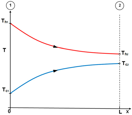
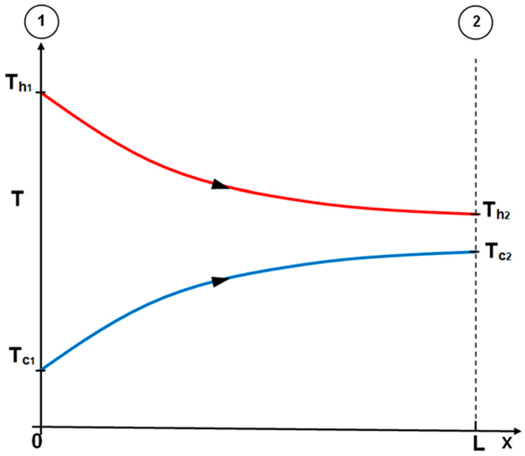
Figure 1 illustrates how the temperatures of both fluid streams vary along the heat exchanger length during co-current operation.
Figure 1.
Changes in temperatures for cold and hot water in a co-current helical heat exchanger; the heat exchanger inlet is marked with the symbol ①, and the outlet with the symbol ②.
Outlet temperatures of hot and cold water were evaluated using the P-NTU approach:
Efficiency is defined as follows:
where the heat transfer unit numbers corresponding to the cold- and hot-water flows are defined as follows:
After calculating the efficiency from Equation (2), the temperature for hot water at the outlet of the heat exchanger is obtained from Equation (1):
By substituting expression (2) into formula (3), the following is obtained:
The rate of heat transported from the hot water, , is equivalent to the rate of heat absorbed by the cold water, :
Transforming Equation (1) gives
After substituting expressions (7) and (8) into Equation (6), one obtains
By performing simple transformations, Equation (10) gives
The outlet temperature of the cold water, , calculated from Equation (6), is expressed by the following formula:
The temperature can alternatively be evaluated using Equation (8):
The P-NTU method is particularly useful for determining the outlet temperatures of hot and cold media for heat exchangers with complex flow configurations. For many types of heat exchanger designs, the appropriate relationships for calculating the efficiency of hot and cold factors can be found in the literature [6]. For calculating the physical properties of water, both hot and cold, arithmetic mean values of inlet and outlet temperatures are used.
3. Experimental Setup and Investigations
The flow and thermal measurements were performed under steady operating conditions. At the heat exchanger inlet, the temperatures of the hot and cold water were maintained constant throughout the measurements. For this reason, a large-capacity hot-water tank with a capacity of 1000L was used. The water was heated in a domestic electric boiler used in central heating systems. Cold water was drawn directly from the municipal water supply network and, after passing through a heat exchanger, was discharged into the sewer system. Due to the large capacity of the municipal water supply network, the temperature of the cold water at the heat exchanger inlet remained constant. The flow rates of both water circuits were controlled by changing the rotational speed of the pumps. Pump speed, expressed in revolutions per minute (rpm), was regulated by means of a frequency converter connected to the power supply.
A computerised data acquisition system was used to collect and store measurement data.
During the experimental tests, particular attention was paid to maintaining constant inlet temperatures throughout a given measurement series. As a result, the heat flow rates determined based on measurements on the hot-water side were equal to the heat flow rates determined based on measurements on the cold-water side. Unlike other methods for determining heat transfer coefficients on the hot and cold fluid sides, such as the Wilson method [1], the water flow rates on the hot and cold sides might vary across successive measurement series, and the flow rate of one fluid need not be constant.
The determination of the HTCs on the hot- and cold-water sides is the inverse heat transfer problem (IHTP). From the m measurement series, the following values are known: hot- and cold-water volume flow rates and at the inlet of the heat exchanger, inlet hot and cold water temperatures and also outlet hot and cold water temperatures.
Based on experimental research, coefficients and exponents will be determined in the assumed form of the heat transfer correlations.
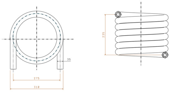
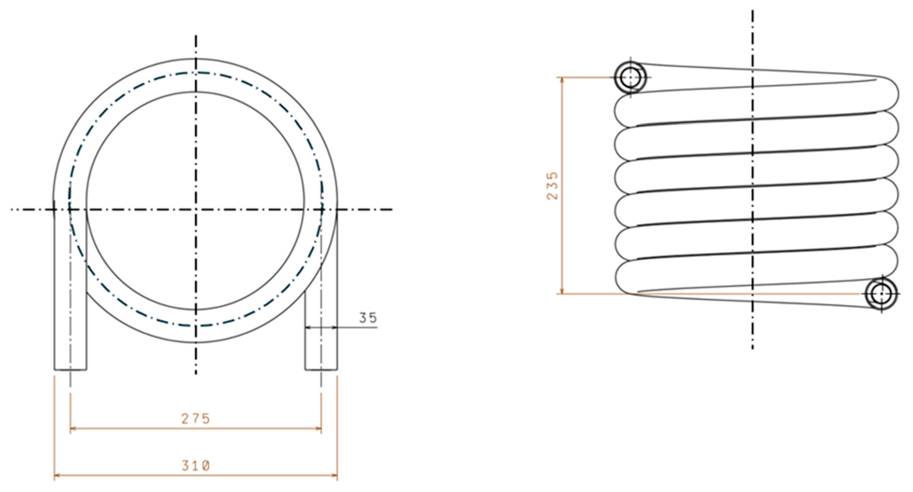
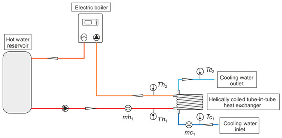
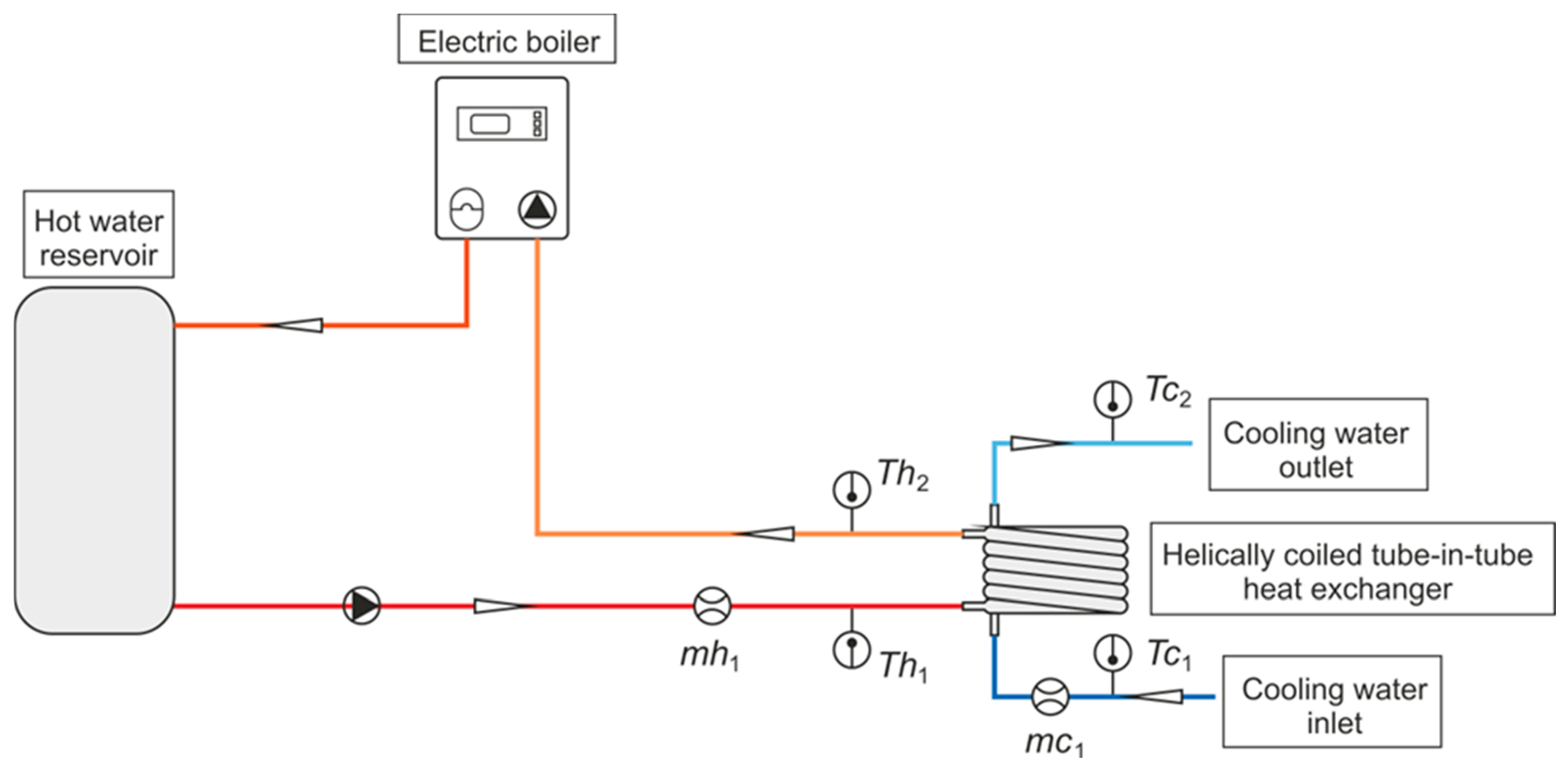
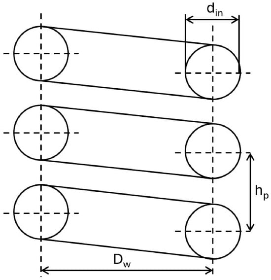
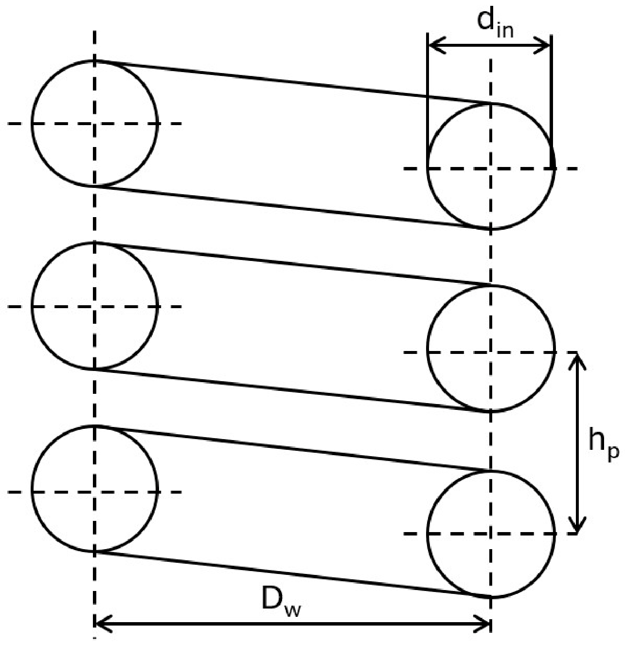
The geometry and dimensions of the tested helically coiled heat exchanger are shown in Figure 2, while the experimental test rig is presented in Figure 3.
Figure 2.
Helically coiled heat exchanger with dimensions.
Figure 3.
Test rig for flow and heat transfer studies of a co-current tube-in-tube coil heat exchanger; and —mass flow rate of the cold water and the mass flow rate of the hot water measured at the inlet of the heat exchanger; —measured water temperature of the cold and hot water at the heat exchanger inlet; —measured water temperature of the cold and hot water at the heat exchanger outlet.
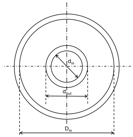
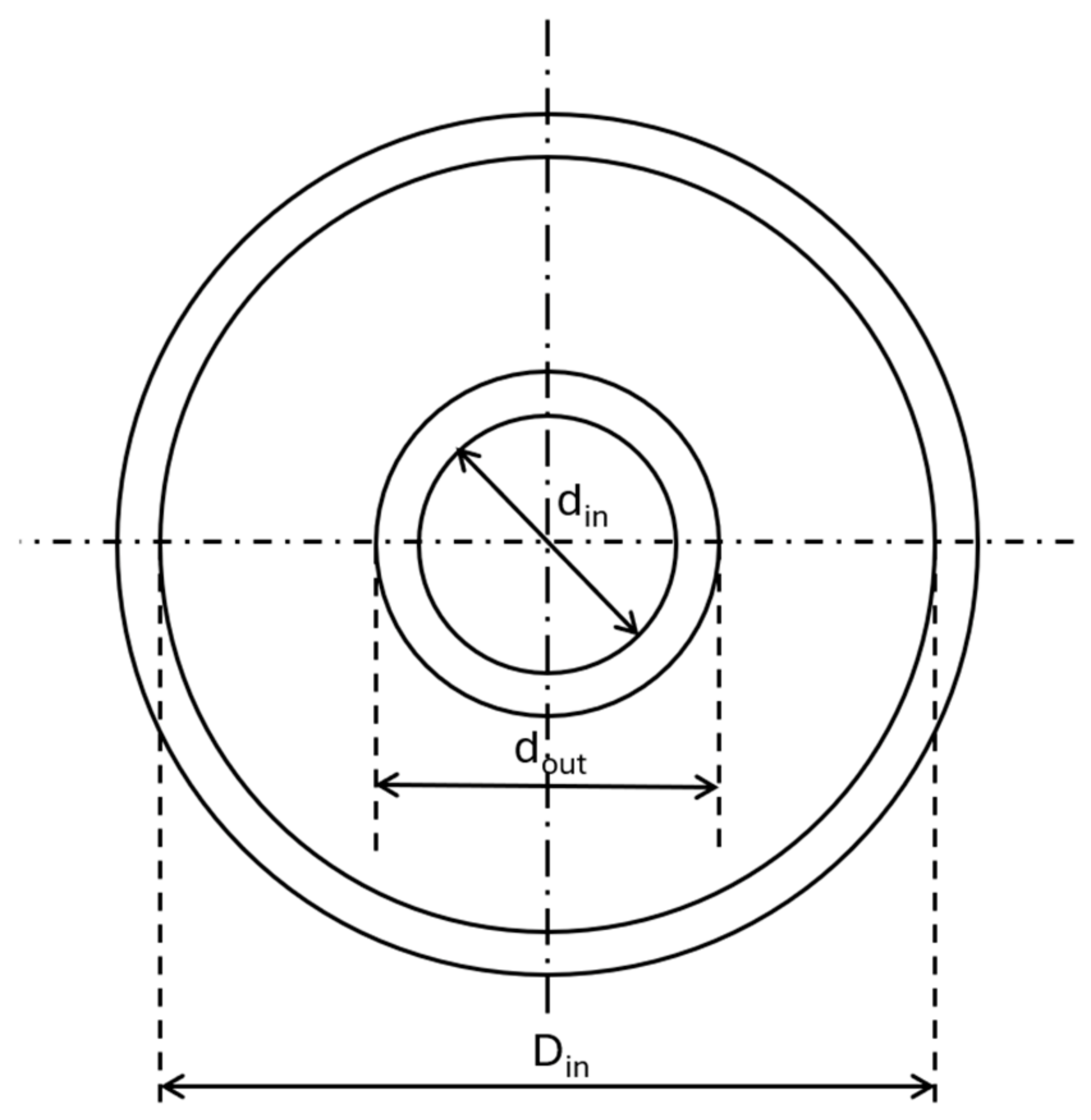
Thermal and flow tests were performed for a tube-in-tube heat exchanger consisting of 6.5 loops. Cold water flows through the annular channel, and hot water flows in the centre tube. The inner diameter Din of the shell tube was 32 mm, and the wall thickness s was equal to 1.5 mm. For the inner tube, the inner diameter din was 20 mm, and the outer diameter dout was 22 mm. The total length of the exchanger was 5.99 m. The diameter of the coil was 275 mm, while its pitch was 70 mm. To avoid energy loss to the environment, the heat exchanger was insulated with polyurethane foam. During the measurement series, the hot-water mass flow rate varied from 0.06 kg/s to 0.33 kg/s, and the cold-water mass flow rate from 0.067 kg/s to 0.13 kg/s. Axial turbine flow meters were employed to monitor the volumetric flow rates of both fluid streams over a measuring range of 2–40 L/min, with an accuracy of ±2% of the indicated value. Temperatures of the hot and cold water at the heat exchanger inlet and outlet were recorded over 53 measurement series. The inlet hot-water temperature ranged from 49.4 °C to 80.9 °C, while the cold-water temperature varied between 9.2 °C and 16.8 °C. Water temperatures were monitored with 1.5 mm-diameter sheathed K-type (NiCr–Ni) thermocouples. Prior to the experiments, each sensor was calibrated using a dedicated calibration furnace. The resulting uncertainty associated with the temperature measurements was estimated at ±0.5 K.
Heat transfer correlations were developed using 4 unknowns: , on the hot-water side and , on the cold-water side.
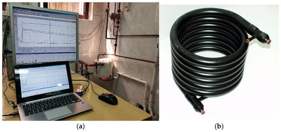
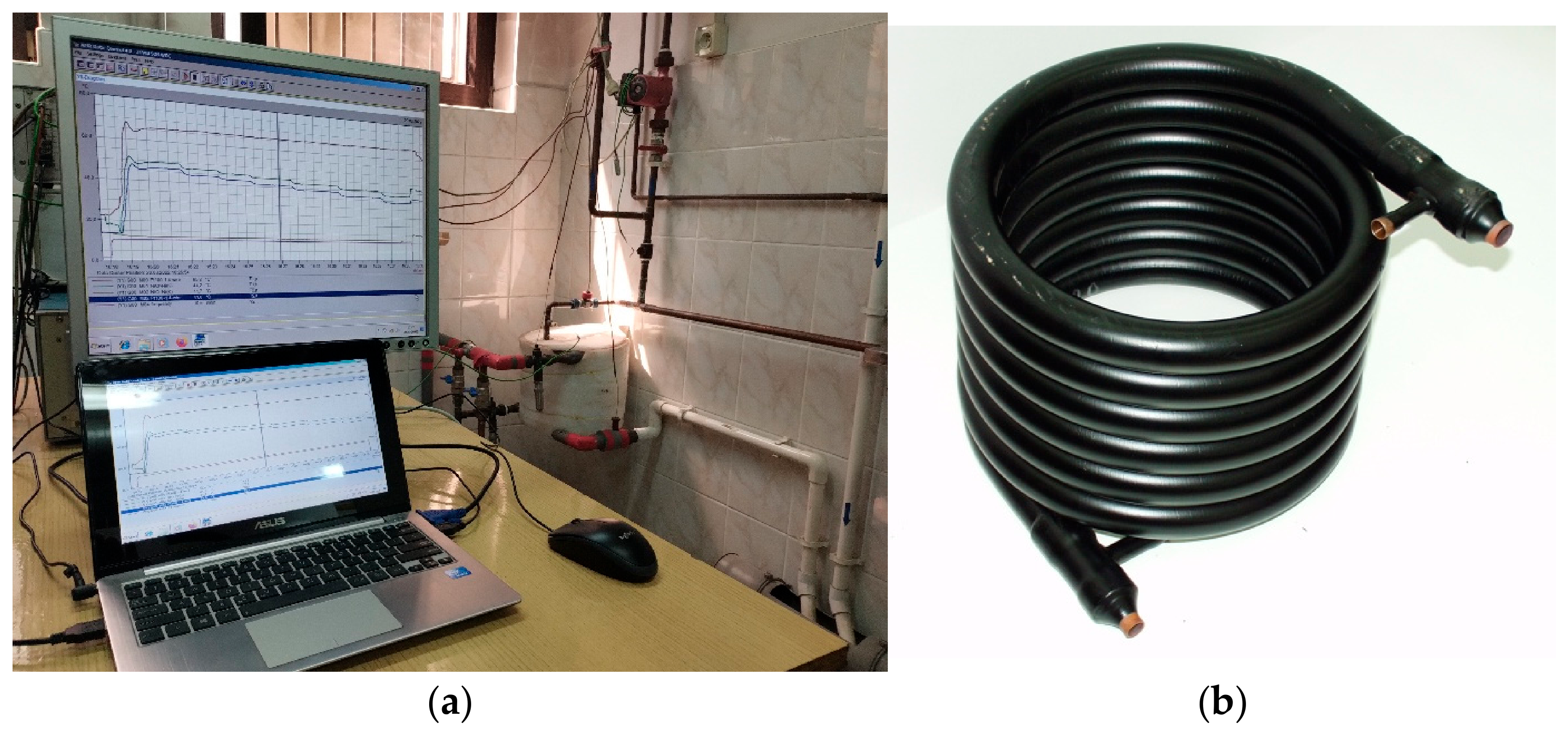
The experimental test rig for the co-current tube-in-tube coil heat exchanger is presented in Figure 4a, and the heat exchanger under test is shown in Figure 4b. On the left-hand side of Figure 4a is a computer, forming an integral part of the computerised data acquisition system. In the bottom right-hand corner is the heat exchanger under test, thermally insulated on its outer surface.
Figure 4.
General view of the test rig for flow and heat transfer studies (a) and view of the tube-in-tube coil heat exchanger under examination (b).
The measured volumetric flow rates, along with the inlet and outlet temperatures of both fluids, are summarised in Table 1.
Table 1.
Measurements including the volumetric flow rates of both hot and cold water, along with their respective temperatures at the exchanger inlet and outlet.
The measured values reported in Table 1 were used to simultaneously identify the unknown coefficients and exponents appearing in the heat transfer relationships for both water flows.
4. Parameter Estimation in Nusselt Number Correlations for Both Water Flows
The following relationship was employed to determine the overall HTC with reference to the external surface area of the inner tube:
Equation (14) is applicable over the entire flow regime, from laminar through transitional to turbulent conditions.
To characterise heat transfer in both flow regions, separate Nusselt number relationships are considered for the flow inside the central tube and for the annular space bounded by the outer wall of the inner tube and the inner wall of the surrounding tube.
Based on several dozen measurement series, unknown parameters were determined in the Nusselt numbers for the hot water flowing in the inner tube and the cold water flowing in the annular channel.
On the basis of the experimental investigations, two unknown parameters, and , in the Nusselt number correlation for the hot-water side were determined. In addition, two parameters, and , were identified for the Nusselt number correlation corresponding to the cold-water side.
The parameter identification procedure begins by establishing the total number n of unknown coefficients appearing in the Nusselt number relationships for the hot- and cold-water streams. For the correlations considered in this study, the number of coefficients to be identified is given by , where specifies the total set of unknown parameters in the Nusselt number correlation for hot water, and represents the total set of unknown parameters for cold water.
In the present study, were adopted, resulting in a total of unknown parameters. These parameters were identified by minimising the sum of squared differences between the calculated and experimentally measured outlet temperatures of the hot and cold water:
The symbols appearing in Equation (15) are defined as follows:
—the total number of experimental series, and —the calculated outlet temperatures of hot and cold water for the i-th measurement series, and —the measured outlet temperatures of hot and cold water for the i-th measurement series.
Temperatures and are functions of the sought parameters .
The Nusselt numbers and on the cold- and hot-water side were subsequently evaluated using the adopted functional forms of the heat transfer relationships, containing unknown coefficients . The coefficients were identified using the least squares procedure, so that the sum given by Equation (15) is minimum. The unknown parameter values were estimated by applying the Levenberg–Marquardt method [30,31,32], which combines the steepest descent method with the Gauss–Newton method. At the beginning of the iterative process, when the values of the sought parameters are far from the values of the parameters at which the sum S reaches its minimum, the steepest descent method is used. In subsequent iterations, when the values of the sought parameters are close to those at which the sum S reaches its minimum, the Gauss–Newton method is employed. The Gauss–Newton algorithm is slow, but allows the parameters to be determined with high accuracy.
The parameters were estimated through successive iterations of the Levenberg–Marquardt algorithm [26,27,28]:
where
The upper index denotes the iteration number, and the weighting factor.
The vectors of the measured and calculated temperatures of hot and cold water at the heat exchanger outlet are as follows:
The Jacobian matrix J is defined as
and evaluated using the finite-difference method.
The symbol In stands for the identity matrix of n × n dimensions, and μ(k) represents the weight factor, modified following the Levenberg–Marquardt algorithm [30,31,32]. The superscript T denotes the transpose of the matrix. Convergence is typically achieved within a small number of iterations. The desired parameters are obtained after just a few to several iterations.
The uncertainties of the estimated parameters in the heat transfer correlations were estimated using the Gauss variance propagation rule. Furthermore, 95% confidence intervals of the determined parameters in the correlations for the Nusselt numbers on the sides of hot and cold water were established. The real values of the determined parameters ,…, are found with a probability of in the following intervals [7]:
where —a parameter determined using the least squares method; —quantile of the t-Student distribution for 95%confidence level; (2m − n)—degree of freedom; —diagonal elements of the variance–covariance matrix.
The least squares sum is characterised by the variance of the fit , which is an estimate of the variance of the data and is calculated according to
where m designates the number of measurement points and n is the number of searched parameters.
The subject matter of the next section is determining heat transfer correlations for calculating the Nusselt number on the hot-water side, i.e., for water flowing in the inner tube.
5. Development of Nusselt Number Correlations for the Hot- and Cold-Water Sides
For laminar flow through the inner tube depicted in Figure 5, the wall Nusselt number was obtained from correlations reported in the literature. Identification of the unknown parameters in the hot-water correlation was restricted to the turbulent regime, defined by , where is the Reynolds number of the hot water flowing through the inner tube and denotes the critical Reynolds number corresponding to the onset of turbulence.
Figure 5.
Configuration of the inner tube forming the helically coiled tube-in-tube heat exchanger.
5.1. Heat Transfer Correlation for Calculating the Nusselt Number on the Inner Surface of the Central Tube for Laminar Flow
Schmidt’s correlation [33] was employed to evaluate the critical Reynolds number corresponding to the onset of turbulent flow:
where (Figure 5)
The following symbols are used in Equations (21) and (22): D—equivalent coil diameter, Dw—average coil diameter, hp—coil pitch, and —internal diameter of the inner coil tube.
Under laminar-flow conditions, the friction factor is given by [34]
where stands for the Reynolds number , —fluid velocity, —density, —kinematic viscosity, and —dynamic viscosity.
The correlation for Nusselt number for laminar flow in a co-current heat exchanger is as follows [23]:
where the constant m is given by
The symbol denotes the Nusselt number for fully developed hydrodynamic and thermal conditions in a straight tube. The Nusselt number for laminar flow is when the wall temperature of the inner tube is constant. The HTC for laminar flow is calculated using the following formula .
In the next Section 5.2, a methodology for establishing the Nusselt number correlation for turbulent flow, based on experimental measurements, will be discussed.
5.2. Heat Transfer Correlation for Calculating the Nusselt Number on the Inner Surface of the Central Tube for Turbulent Flow
Heat transfer correlations for the turbulent flow of hot water were determined based on the experimental data reported in Table 1.
Initially, the form of the function for calculating Nusselt numbers on both the inner and outer surfaces of the inner tube should be specified. The mathematical formula for calculating the Nusselt number for straight tubes is [35]
with the Darcy–Weisbach friction factor calculated according to [36]
Correlation (26) cannot be directly applied to a coil due to the complex fluid flow in the cross-section [9]. The friction coefficient is also higher in a coil compared to a straight tube. The friction coefficient for a coil is determined by the formula [34]
The analysis of Equation (28) reveals that the friction coefficient is the sum of the friction coefficient for a smooth-walled tube, calculated using the Blasius formula [37], and a term accounting for flow in the coil.
Three alternative correlation forms were considered to describe the dependence of the Nusselt number on the Reynolds and Prandtl numbers, each of which calculated the friction coefficient using formula (28). Using the experimental data presented in Table 1, the following correlations were obtained for calculating the Nusselt number.
- First correlation for hot water
For the heat exchanger under study, the lower limit of the range of validity of Equation (29) is set by the critical Reynolds number .
The following values of the parameters were identified using the minimum sum-of-squares criterion (Equation (15)):
The minimised sum of squared residuals is , whereas the corresponding mean squared error is
The uncertainty associated with the identified parameters was quantified by constructing 95% confidence intervals according to the Gauss variance propagation approach [7], yielding the following ranges:
- Second correlation for hot water
The following values of the parameters were identified using the minimum sum-of-squares criterion (Equation (15)):
The minimised sum of squared residuals is , whereas the corresponding mean squared error is
The uncertainty associated with the identified parameters was quantified by con-structing 95% confidence intervals according to the Gauss variance propagation approach [7], yielding the following ranges:
- Third correlation for hot water
The parameter values listed below were determined based on the minimum sum-of-squares condition (Equation (15)):
The minimised sum of squared residuals is , whereas the corresponding mean squared error is
The uncertainty associated with the identified parameters was quantified by con-structing 95% confidence intervals according to the Gauss variance propagation approach [7], yielding the following ranges:
An analysis of Equations (29)–(37) shows that the determined values and are very similar for all three determined correlations. Minor differences in the determined values and are attributed to variations in the correlations applied for the Nusselt number on the cold-water side flowing through the annular channel.
The analysis that follows focuses on developing Nusselt number correlations for the cold-water flow through the annular passage.
5.3. Nusselt Number Correlation for Turbulent Flow in the Annular Channel
As illustrated in Figure 6, the cold-water stream passes through the annular passage. The Nusselt number relationships for this flow region were formulated using Equation (26), originally established for flow in a straight circular tube, as the reference form. The friction coefficient for cold water was calculated using the relationship proposed by Xin et al. [38]:
Figure 6.
Cross-section of helically coiled heat exchanger.
The corresponding Reynolds and Dean numbers are calculated using the following expressions:
The symbols in Equation (39) designate the following: —fluid velocity, —density, —kinematic viscosity, and —dynamic viscosity.
Hydraulic equivalent diameter is given by
where denotes the cross-sectional area of the annular channel, and represents its wetted perimeter.
The Nusselt number on the cold-water side was approximated using three different correlations:
- First correlation for cold water
The following parameter values were identified using the minimum sum-of-squares criterion (Equation(15)):
The minimised sum of squared residuals is , whereas the corresponding mean squared error is
The uncertainty associated with the identified parameters was quantified by constructing 95% confidence intervals according to the Gauss variance propagation approach [7], yielding the following ranges:
- Second correlation for cold water
The following parameter values were identified using the minimum sum-of-squares criterion (Equation(15)):
The minimised sum of squared residuals is , whereas the corresponding mean squared error is
The uncertainty associated with the identified parameters was quantified by constructing 95% confidence intervals according to the Gauss variance propagation approach [7], yielding the following ranges:
- Third correlation for cold water
Minimization of the sum-of-squares objective function defined by Equation (15) yielded the following parameter estimates:
The minimised sum of squared residuals is , whereas the corresponding mean squared error is
The uncertainty associated with the identified parameters was quantified by constructing 95% confidence intervals according to the Gauss variance propagation approach [7], yielding the following ranges:
6. Discussion of the Results
The Nusselt number correlations on the hot and cold-water sides are highly accurate. The minimum sum of squares was 8.10 K2, despite the large number of measurement series, indicating a close match between the calculated and experimentally measured temperatures at the heat exchanger outlet. Table 2 presents the temperatures of hot and cold water at the outlet of the heat exchanger, both calculated and measured, along with the relative differences between them.
Table 2.
Comparison of predicted and experimental outlet temperatures for the hot- and cold-water streams, including their relative deviations.
The differences and between the measured values and the corresponding model predictions presented in Table 2, expressed as relative values, were determined using the following equations:
The agreement between the measured and calculated values was additionally assessed using the root mean square error (RMSE), defined as
where (n) is the number of measurement series, is the calculated value, and is the corresponding measured value.
Analysis of the data in Table 2 indicates a very close correspondence between the predicted outlet temperatures and the corresponding experimental values. The maximum absolute relative deviation observed is 1.01% for the cold water and 2% for the hot water.
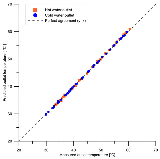
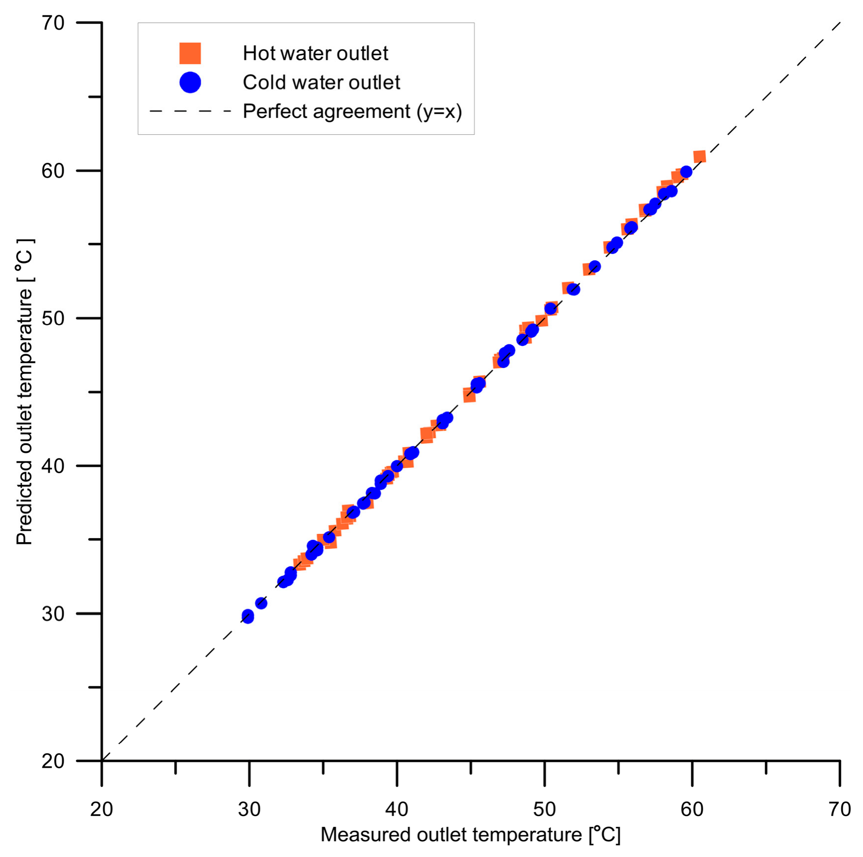
To provide a graphical assessment of the agreement between the experimental measurements and the model predictions, Figure 7 compares the measured and calculated outlet temperatures of the hot- and cold-water streams for all 53 measurement series. The dashed line represents perfect agreement between the measured and calculated values. The root mean square error (RMSE), calculated using the data presented in Table 2, is 0.197 K for the cold water and 0.334 K for the hot water. The results indicate good agreement between the measured and calculated outlet temperatures over the investigated operating conditions.
Figure 7.
Comparison of measured and calculated outlet temperatures for hot and cold water for 53 experimental measurement series. The dashed line represents perfect agreement (y = x).
For the 53 measurement series listed in Table 3, the heat transfer rates were evaluated separately from the measurements obtained for the hot and cold flows using the following expressions:
Table 3.
Experimental and predicted heat transfer rates for both water flows, including deviations relative to their respective mean values.
Relative deviations between the heat flow rates achieved from the hot- and cold-water sides and the corresponding average rates of heat flow were evaluated according to the following expressions:
Between the differences and , a relationship exists: .
The predicted heat flow rates for the hot- and cold-water sides are equal:
The relative difference between the experimental and predicted mean heat flow rates were calculated from the equation
In Equations (50)–(53), the following notation is adopted: , , —the heat flow rates associated with the cold and hot flows and their mean value, respectively, for the i-th measurement series; —heat flow rate evaluated from the cold- or hot-water data for the i-th experimental series; , —the discrepancy between the experimentally obtained heat flow rates and and the average value for the i-th measurement series; —the deviation between the measured mean heat flow rates and calculated .
The results summarized in Table 3 demonstrate close consistency between the experimental and calculated heat flow rates on both the hot- and cold-water sides. At most operating points, the hot- and cold-side values remain within of the corresponding mean heat flow rate. Furthermore, the model predictions for heat transfer between the two flows agree closely with the mean values derived from the experimental data, with the largest relative discrepancy being only 2.04%.
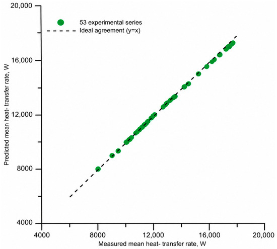
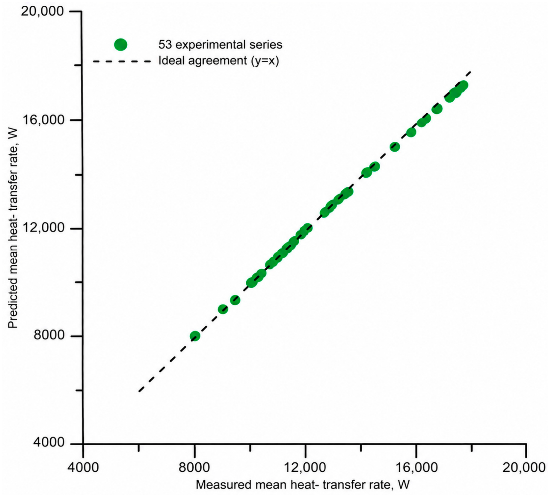
Figure 8 compares the experimental and calculated heat transfer rates for all 53 measurement series. The experimental heat transfer rate was taken as the mean of the values determined from the energy balances of the hot- and cold-water streams. The dashed line represents perfect agreement between the experimental and calculated values. The root mean square error (RMSE) was 143.44 W, confirming the close agreement between the experimental results and the model predictions.
Figure 8.
Comparison of experimental and calculated heat transfer rates for 53 measurement series. The dashed line represents perfect agreement (y = x).
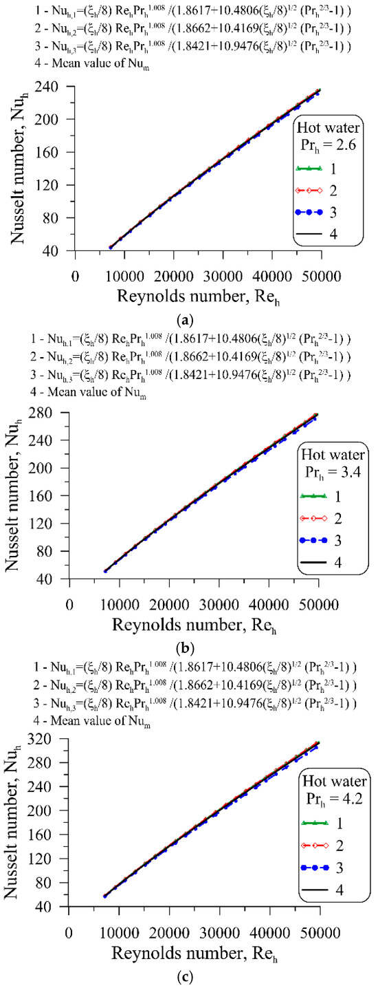
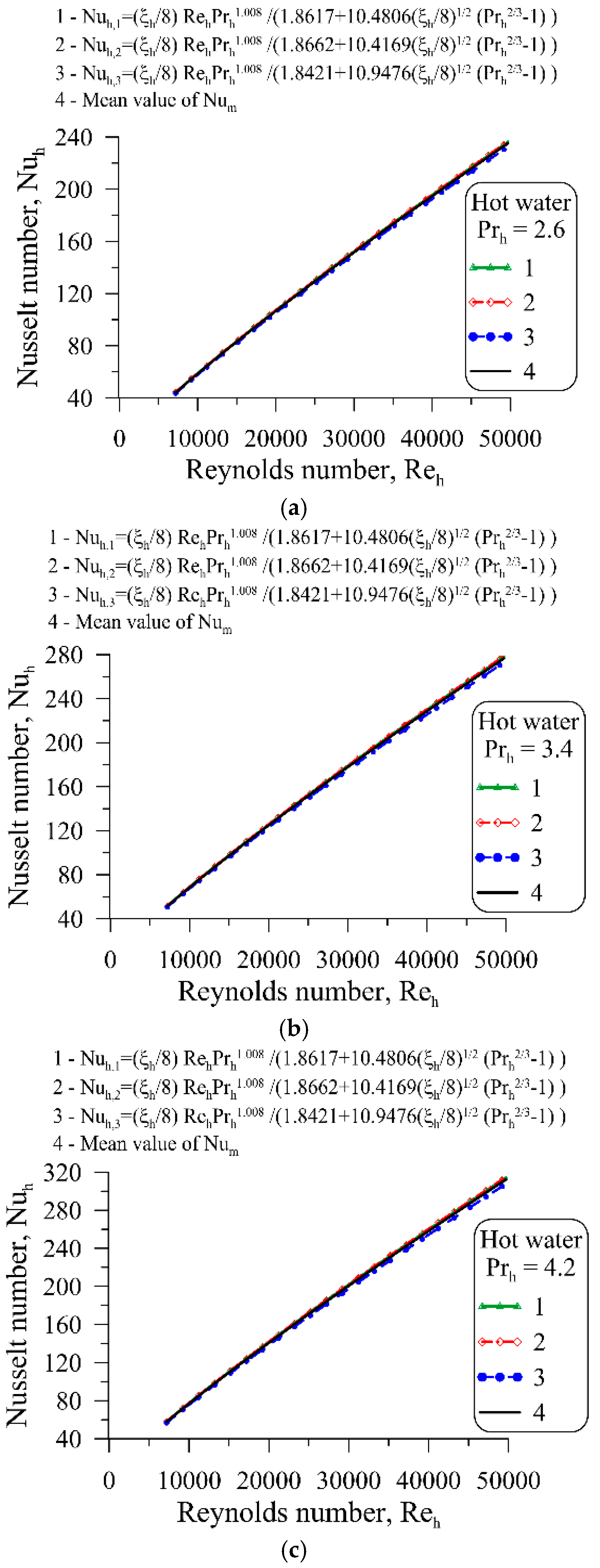
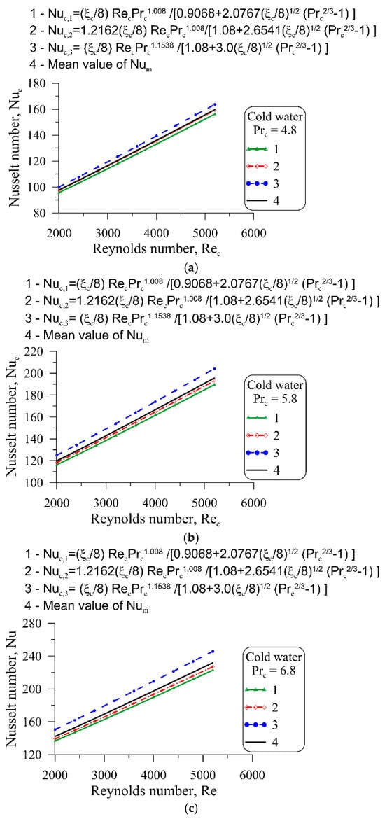
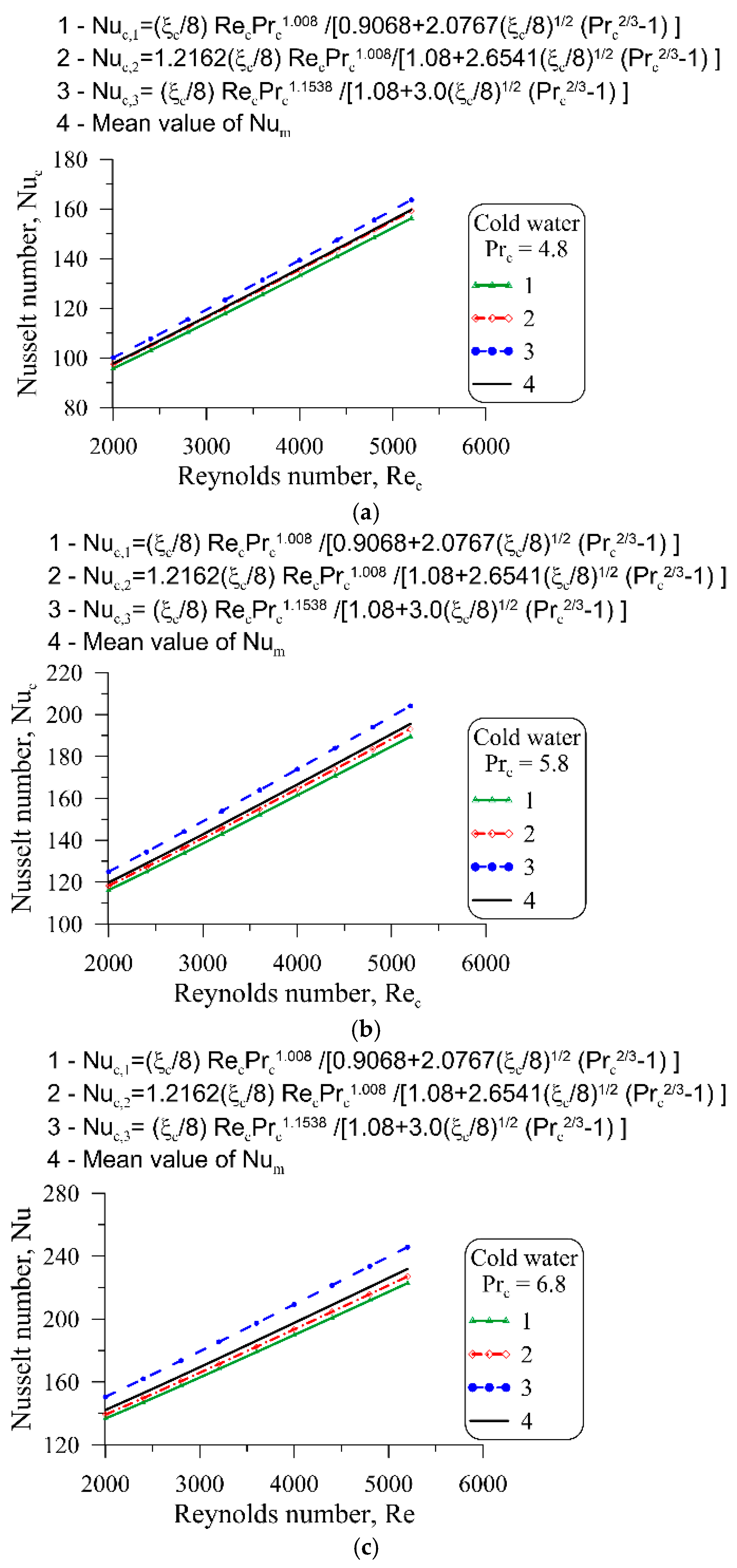
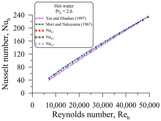
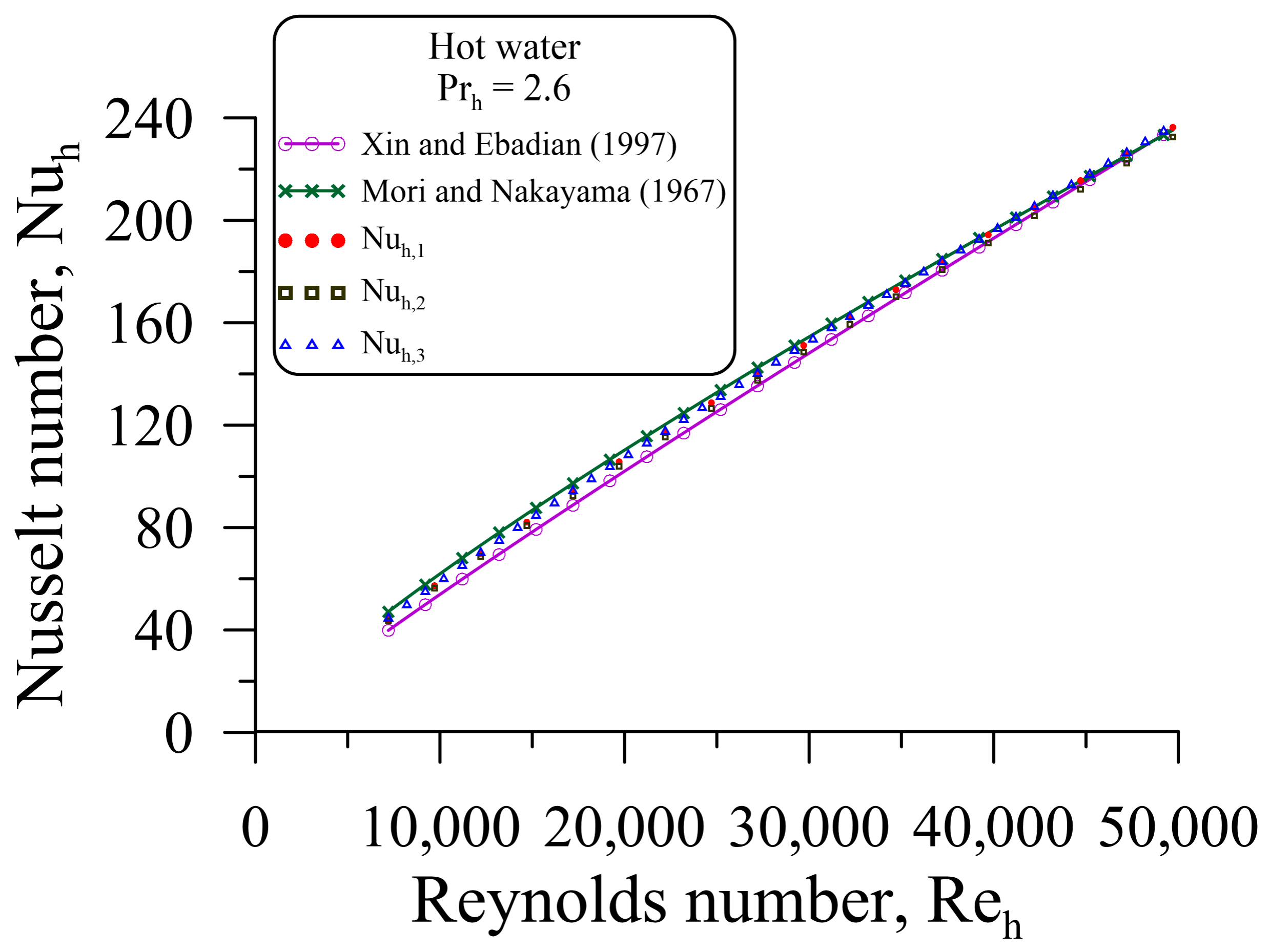
Figure 9 and Figure 10 show changes in the Nusselt number as a function of the Reynolds number for hot and cold water, respectively. Figure 9 and Figure 10 also depict the average values of the Nusselt number calculated using the following formula
where , , denote the Nusselt numbers calculated for a given Reynolds number using three different correlations determined using experimental data.
Figure 9.
Hot-side Nusselt number correlations at selected Prandtl numbers: (a) Pr = 2.6, (b) Pr = 3.4, and (c) Pr = 4.2.
Figure 10.
Cold-side Nusselt number correlations at selected Prandtl numbers: (a) Pr = 4.8, (b) Pr = 5.8, and (c) Pr = 6.8.
As can be observed from Figure 9 and Figure 10, the Nusselt numbers predicted by the three different correlations are in close agreement. This indicates good accuracy of the measurement data and the correct form of the function approximating the experimentally determined Nusselt numbers, , .
The relative differences , , and , , were calculated using the following formulas:
The relative difference , given by Equation (56), represents the relative difference between the average Nusselt number calculated from formula (55) and the correlation number for the Nusselt number determined on the basis of experimental studies. The relative differences and were calculated in a similar manner using Equations (57) and (58).
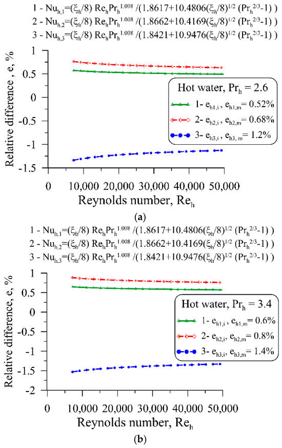
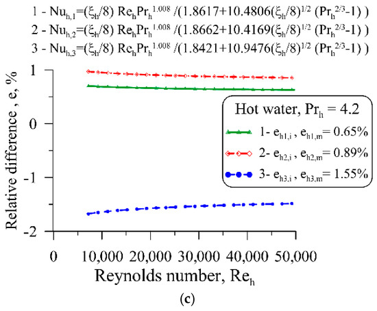
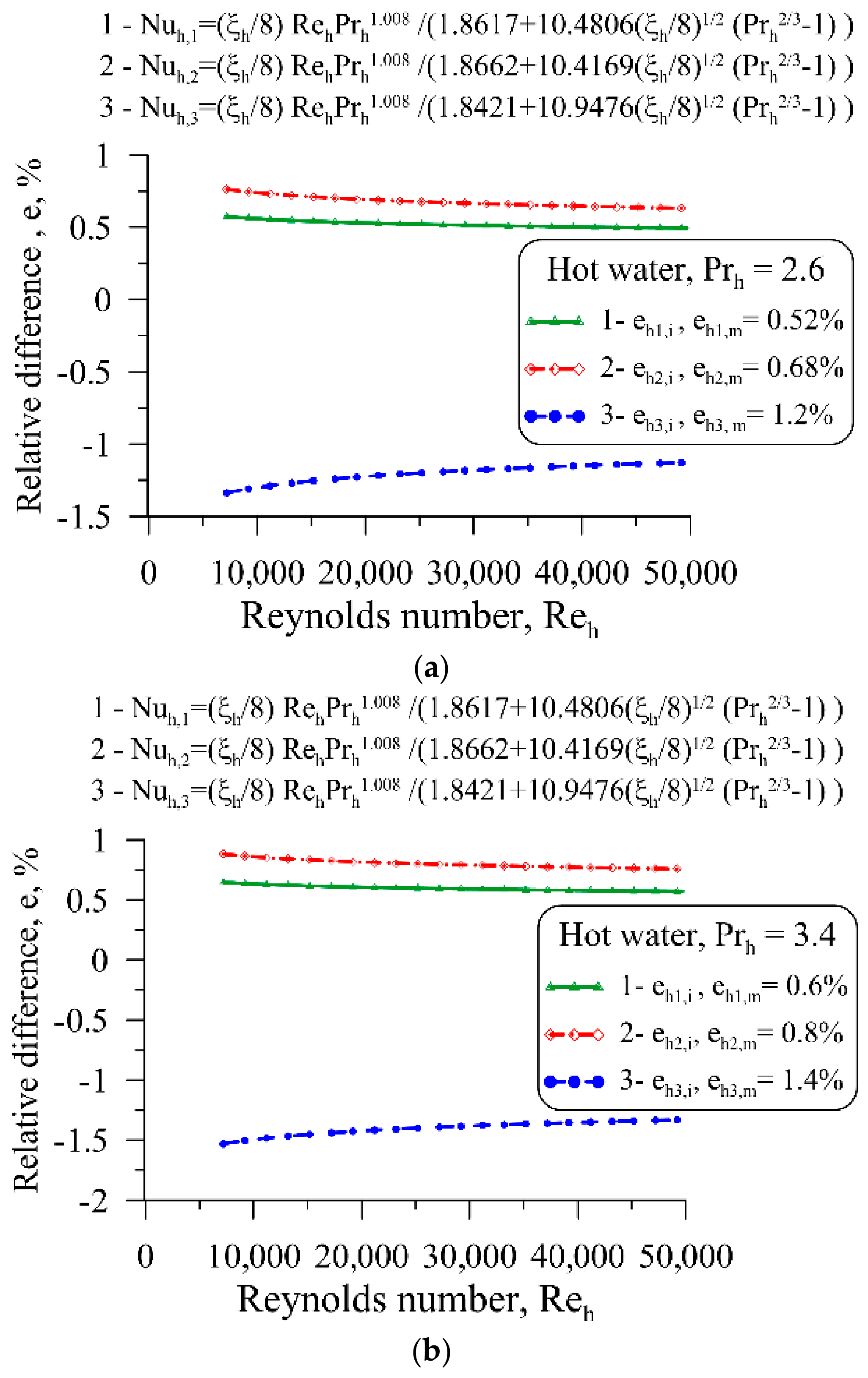
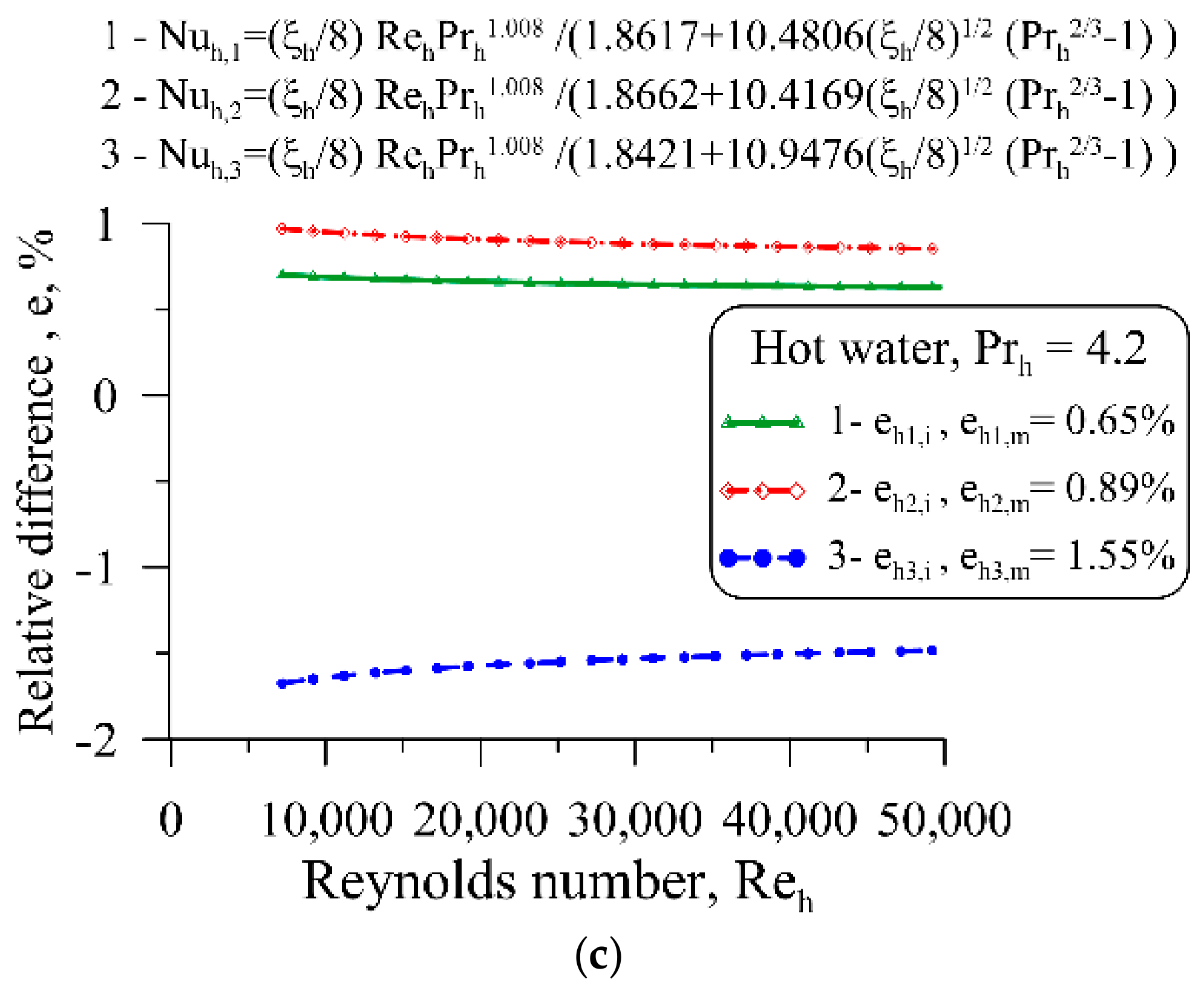
An analysis of the results presented in Figure 11 shows that the relative differences , , , are small for all Prandtl numbers. Also, the values of the average relative differences , and are small and range from 0.52% (Figure 9a) to 1.55% (Figure 9c).
Figure 11.
Relative differences , , , and average relative differences calculated from Formulas (56)–(58) for Nusselt numbers , , , which are presented in Figure 9, for different Prandtl numbers: (a) Pr = 2.6, (b) Pr = 3.4, and (c) Pr = 4.2.
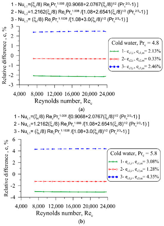
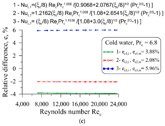
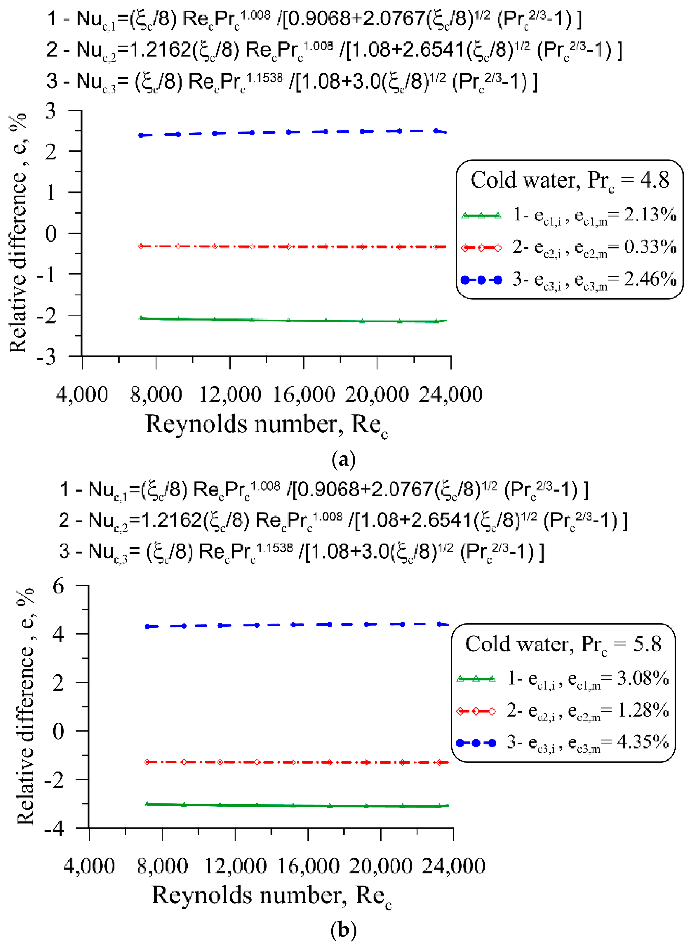
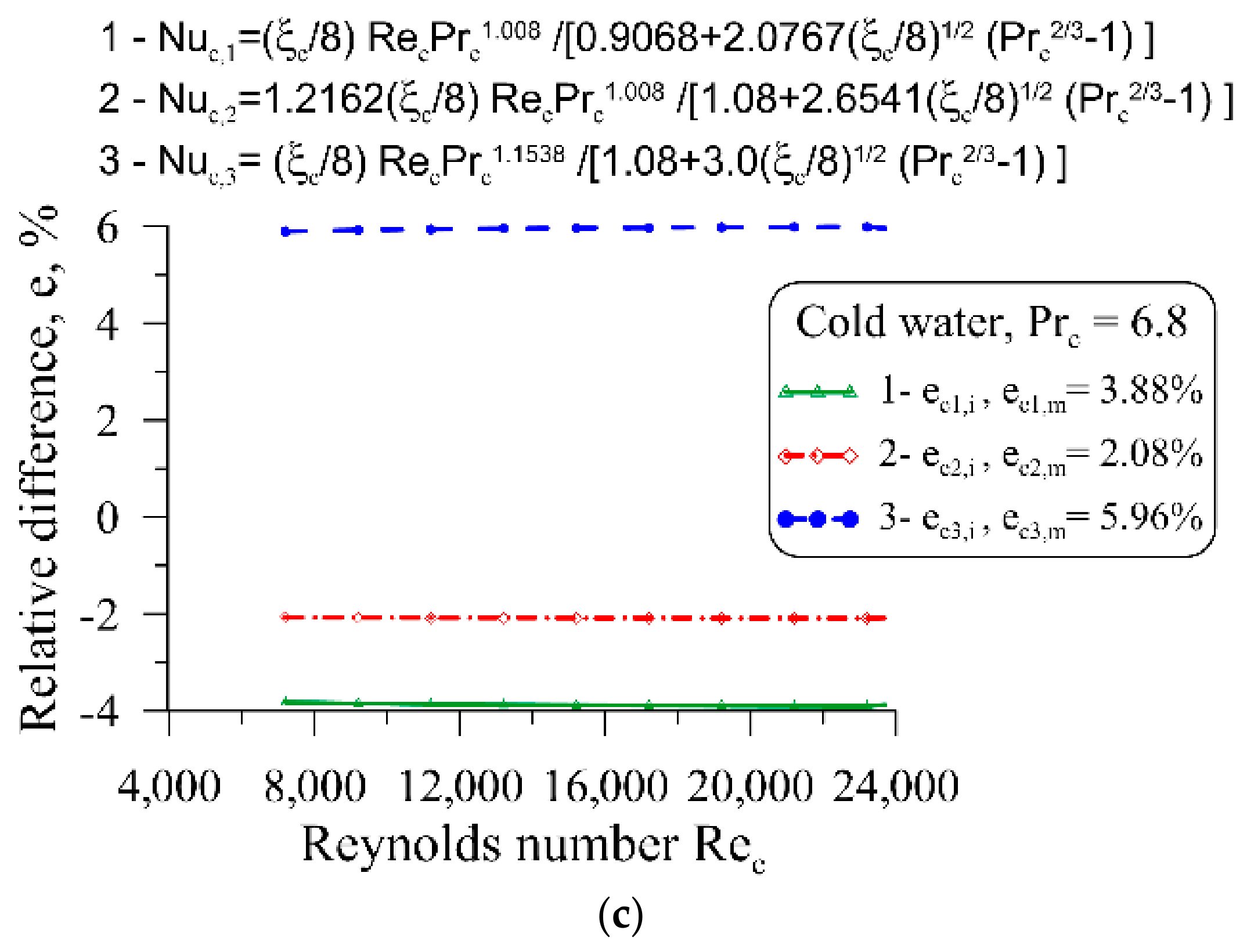
Figure 12 shows graphs of relative differences for cold water flowing in a ring channel, analogous to Figure 11.
Figure 12.
Relative differences , , , and average relative differences calculated from Formulas (56)–(58) for Nusselt numbers , , , which are presented in Figure 10.
The results presented in Figure 10 indicate that the relative deviations , , , are small for all Prandtl numbers. Also, the values of the average relative differences , and are small and range from 0.33% (Figure 12a) to 5.96% (Figure 12c).
The values of relative differences , , , and relative differences of averages , , determined for cold water are greater than the corresponding values determined for hot water. This is due to the more complex flow and thermal phenomena occurring in the annular channel through which cold water flows, compared to the more orderly flow occurring in the coil (central tube).
The correlations determined for hot water, given by Equations (29), (32), and (35) were compared in Figure 13 with the correlation of Mori and Nakayama [22]:
and Xin and Ebadian [24]:
Figure 13.
Comparison of correlations determined for hot water with correlations found in the literature [22,24].
The data presented in Figure 13 indicate that the Nusselt numbers calculated using the correlations determined in the article differ only slightly from the Nusselt numbers determined using Equations (59) and (60).
Additionally, the HTC calculated using Equation (14) was compared with the HTCs determined experimentally from the formula
where the heat exchange surface area was calculated using the formula . The symbol L denotes the length of the inner tube.
Inspection of the results presented in Table A1 (Appendix A) shows high accuracy in determining the HTC and for the hot- and cold-water sides, respectively. The heat transfer coefficients and differ only slightly. For most measurement series, the relative difference between these coefficients does not exceed a few per cent.
The new and original elements presented in the paper are as follows:
- New, comprehensive results of an experimental study on helical coiled heat exchangers are presented.
- New correlations for Nusselt number prediction are determined simultaneously on both the cold- and hot-water sides. In the existing literature, correlations are generally determined for only one side of the partition; for example, a correlation for the Nusselt number on one side of the partition (such as that for a straight tube) is taken from the literature, while only the unknown coefficients and exponents in the correlation for the other side of the partition are determined. This approach usually leads to significant inaccuracies, as errors in determining the heat transfer coefficient, calculated using Nusselt correlations from the literature for straight tubes, often result in low accuracy in the correlation determined on the other side of the partition.
- The paper proposes new forms of correlations for determining the Nusselt number in an internal tube (hot fluid), given by Equations (29), (32) and (35), and new correlations for an annular channel (cool fluid), given by Equations (41), (44) and (47).
- The Nusselt number correlations (29) and (30), (32) and (33), (35) and (36) derived in this paper for a hot tube flowing through an inner tube, and the correlations for an annular channel (41) and (42), (44) and (45), (47) and (48), are new and characterised by very good accuracy, as confirmed by the detailed analyses carried out in this article.
- Correlations (41) and (42), (44) and (45), and (47) and (48) are particularly valuable for cold water flowing through an annular channel, considering the lack of suitable, experimentally verified correlations for calculating the Nusselt number in the available literature.
7. Conclusions
This study introduces a novel experimental approach for evaluating the thermal performance of a helically coiled tube-in-tube heat exchanger. The experimental flow and temperature data were subsequently used to develop separate Nusselt number relationships for the hot- and cold-water sides. Heat exchangers of this type are used as evaporators and condensers in heat pumps. The paper provides expressions for calculating the Nusselt number on both the cold- and hot-water sides with high accuracy. This enables the correct calculation of the dimensions of the heat transfer surface (tube length and diameters) in design calculations, and a more accurate determination of the outlet temperatures of both fluids in performance calculations. An additional advantage of the methodology proposed in this work and the correlations derived is particularly important in high-temperature heat exchangers, where the wall temperature of the inner tube must be known. Unlike the popular Wilson method used to iteratively develop Nusselt number correlations for both cold and hot fluid sides, successive measurement series may differ in both volumetric flow rates and inlet and outlet temperatures. There is no need to maintain a constant HTC on one side of the tube wall when the flow and thermal conditions on the other side change, as is typical in the Wilson method. Furthermore, there is no need to use power functions to approximate Nusselt numbers as a function of Reynolds and Prandtl numbers, as is the case with the Wilson method. An important feature of the proposed method is the determination of unknown parameters in the correlations for Nusselt numbers using the nonlinear least-squares method, thereby ensuring high accuracy in the resulting correlations. The Wilson method linearises power functions, allowing linear regression to determine the desired parameters in the correlations for Nusselt numbers. In the proposed method, the only important condition is to maintain the heat exchanger at steady state in each measurement series. The formula for the Nusselt number for an internal tube through which hot water flows is analogous to the formula for the Nusselt number for a straight tube. It should be noted that the formula for the Nusselt number for a straight tube was derived from a numerical solution of the momentum and energy conservation equations for turbulent flow in a straight tube. The correlations for the Nusselt number determined for the internal coil are more accurate, whereas those for the annular channel formed by the external and internal tubes are slightly less accurate.
The flow and heat measurements carried out on the co-current coil heat exchanger exhibit very good accuracy. Only minor discrepancies were observed between the experimental and predicted heat transfer rates for both water sides. Only minor differences were found between the heat transfer rates evaluated for the hot and cold water. For most operating points, the values obtained for either fluid remained close to the corresponding experimental mean. Moreover, the model predictions closely reproduced the mean heat transfer rates derived from the measurements. The maximum relative discrepancy did not exceed approximately 2%.
The correlations for Nusselt numbers also do not differ significantly from one another. At a fixed Reynolds number, deviations of the individual Nusselt number predictions from their mean values remain within 0.52–1.55% for hot water, whereas a wider range of 0.33–5.96% is obtained for cold water.
8. Limitations of Experimental Determination of Heat Transfer Correlations and Future Work
It should be emphasised that it is of utmost importance to conduct the tests under steady-state conditions. In other words, during a given series of measurements, the heat exchanger must remain in a steady state. Furthermore, experimental studies should ensure good agreement between the heat flow rate transferred from the hot medium and the heat flow rate absorbed by the cold medium. The heat exchanger should be well insulated on its outer surface.
Accurate prediction of the Nusselt number requires a suitable functional dependence on both the Reynolds and Prandtl numbers. Conventional power-law expressions may become inadequate when the Prandtl number varies over a broad range, as their mathematical form does not always represent its influence on heat transfer with sufficient accuracy. Examination of several alternative formulations showed that an inappropriate correlation structure results in markedly larger discrepancies between the experimental and predicted outlet temperatures.
The applicability of the proposed Nusselt number correlations is limited by the ranges of the Reynolds and Prandtl numbers covered by the experimental measurements. Since the correlation parameters were identified using a restricted set of operating conditions, their reliability has been demonstrated only within the investigated ranges. In particular, the fitted relationships may not adequately represent changes in the flow structure or heat transfer mechanisms occurring at Reynolds numbers outside the experimental range. Similarly, extrapolation to substantially different Prandtl numbers may lead to inaccurate predictions because the influence of fluid properties has not been verified beyond the conditions considered in this study. Therefore, the proposed correlations should not be extrapolated beyond the investigated Reynolds- and Prandtl-number ranges without additional experimental validation. Further studies covering a wider range of flow rates and fluid temperatures are required to assess their broader applicability.
The developed methodology enables the simultaneous identification of Nusselt number correlations for both fluid flows and can be applied to a broad range of heat exchanger configurations, such as shell-and-tube, plate, and spiral units. Its applicability is not restricted to a particular heat transfer surface geometry, as both unfinned and finned tubes or plates, including surfaces with discrete or continuous fins, may be considered. The outlet temperatures of the two fluid flows required in the parameterestimation procedure may be obtained using the P-NTU approach, numerical heat exchanger models, or CFD simulations performed with commercial software.
The developed methodology is also applicable to test exchangers manufactured by 3D printers [39]. Printed heat exchangers can have complex heat transfer surface shapes; for example, they can be minimal surfaces such as the Schoen Gyroid, Schwartz Diamond, and Schwartz Primitive.
Author Contributions
Conceptualisation, E.Z. and D.T.; methodology, D.T. and J.T.; software, E.Z. and J.T.; validation, D.T. and T.S.; formal analysis, E.Z. and T.S.; investigation, J.T. and T.S.; data curation, E.Z., D.T. and T.S.; writing—original draft, E.Z.; writing—review & editing, D.T.; visualisation, E.Z.; supervision, D.T. All authors have read and agreed to the published version of the manuscript.
Funding
This research received no external funding.
Data Availability Statement
The original contributions presented in this study are included in the article. Further inquiries can be directed to the corresponding authors.
Conflicts of Interest
The authors declare no conflicts of interest.
Appendix A
Table A1.
A summary of the calculation results and a comparison of the HTCs and obtained with the developed approach and using the logarithmic mean temperature difference.
References
- Wilson, E.E. A basis for rational design of heat transfer apparatus. Trans. ASME 1915, 37, 47–70. [Google Scholar] [CrossRef] [Scilit]
- Fu, Y.; Bian, B.; Liu, Y.; Zhang, L.; Li, M.; Wen, J.; Xu, G. Airside heat transfer analysis using Wilson plot method of three analogous serpentine tube heat exchangers for aero-engine cooling. Appl. Therm. Eng. 2024, 248, 123238. [Google Scholar] [CrossRef] [Scilit]
- Gnielinski, V. New equations for heat and mass transfer in turbulent pipe and channel flow. Int. Chem. Eng. 1976, 16, 359–368. [Google Scholar]
- Petukhov, B.S. Heat transfer and friction in turbulent pipe flow with variable physical properties. In Advances in Heat Transfer; Hartnett, J.P., Irvine, T.F., Eds.; Academic Press: New York, NY, USA, 1970; Volume 6, pp. 503–564. [Google Scholar]
- Taler, D. Prediction of heat transfer correlations for compact heat exchangers. Forsch. Ingenieurwesen 2005, 69, 137–150. [Google Scholar] [CrossRef] [Scilit]
- Nguyen, D.H.; Kim, T.; Kim, J.M.; Kim, T.; Arkadumnuay, T.; Mahian, O.; Ahn, H.S.; Wongwises, S. Enhancing the vertical downward condensation heat transfer of a plate heat exchanger by electrochemical etching. Int. J. Heat Mass Transf. 2024, 225, 125277. [Google Scholar] [CrossRef] [Scilit]
- Taler, D. Experimental determination of correlations for average heat transfer coefficients in heat exchangers on both fluid sides. Heat Mass Transf. 2013, 49, 1125–1139. [Google Scholar] [CrossRef] [Scilit]
- Taler, D.; Ziółkowska, E.; Taler, J.; Sobota, T.; Jaremkiewicz, M.; Marcinkowski, M.; Cieślik, T. Experimental-numerical method for determining heat transfer correlations in the plate-and-frame heat exchanger. Energies 2025, 18, 4760. [Google Scholar] [CrossRef] [Scilit]
- Taler, D.; Taler, J. Simple heat transfer correlations for turbulent tube flow. E3S Web Conf. 2017, 13, 02008. [Google Scholar] [CrossRef] [Scilit]
- Lee, H.; Sadeghianjahromi, A.; Kuo, P.L.; Wang, C.C. Experimental investigation of the thermofluid characteristics of shell-and-plate heat exchangers. Energies 2020, 13, 5304. [Google Scholar] [CrossRef] [Scilit]
- Welty, J.R.; Rorrer, G.L.; Foster, D.G. Fundamentals of Momentum, Heat and Mass Transfer, 6th ed.; Wiley: Hoboken, NJ, USA, 2018. [Google Scholar]
- Seol, S.H.; Lee, S.G.; Son, C.H.; Yoon, J.H.; Eom, I.S.; Park, Y.M.; Yoon, J.I. Effects of experimental parameters on condensation heat transfer in plate fin heat exchanger. Energies 2021, 14, 7681. [Google Scholar] [CrossRef] [Scilit]
- Zhang, J.; Wu, J.; Zhou, H.; Yu, J.; Zhang, B.; Li, W.; He, Y. Condensation heat transfer efficiency analysis of horizontal double-sided enhanced tubes. Energies 2025, 18, 2390. [Google Scholar] [CrossRef] [Scilit]
- Xiang, H.; Du, W.; Zhao, J. Numerical investigation on the thermal-hydraulic performance of high Prandtl number fluid in offset strip fin with different offset. Int. J. Heat Mass Transf. 2023, 220, 124915. [Google Scholar] [CrossRef] [Scilit]
- Noor, H.H.; Shaaban, S.M.; Alazzam, M.B.; El-Rahman, A.A.; Alhumaid, S.; Mehdar, Y.T.H.; Ali, E.S. Numerical evaluation of the influence of various fluid types on the efficiency of distinctively designed shell-and-spiral tube heat exchangers. Case Stud. Therm. Eng. 2025, 76, 107226. [Google Scholar] [CrossRef] [Scilit]
- Kim, K.; Song, K.S.; Lee, G.; Chang, K.; Kim, Y. Single-phase heat transfer characteristics of water in an industrial plate and shell heat exchanger under high-temperature conditions. Energies 2021, 14, 6688. [Google Scholar] [CrossRef] [Scilit]
- Xu, X.; Liu, C.; Dang, C.; Wu, Y.; Liu, X. Experimental investigation on heat transfer characteristics of supercritical CO2 cooled in horizontal helically coiled tube. Int. J. Refrig. 2016, 67, 190–201. [Google Scholar] [CrossRef] [Scilit]
- Lei, Z.; Bao, Z. Experimental investigation on laminar heat transfer performances of RP-3 at supercritical pressure in the helical coiled tube. Int. J. Heat Mass Transf. 2022, 185, 122326. [Google Scholar] [CrossRef] [Scilit]
- Liu, P.; Wang, R.; Liu, S.; Bao, Z. Experimental study on the thermal-hydraulic performance of a tube-in-tube helical coil air–fuel heat exchanger for an aero-engine. Energy 2023, 267, 126626. [Google Scholar] [CrossRef] [Scilit]
- Mori, Y.; Nakayama, W. Study of forced convective heat transfer in curved pipes (2nd report, turbulent region). Int. J. Heat Mass Transf. 1967, 10, 37–59. [Google Scholar] [CrossRef] [Scilit]
- Kreith, F.; Manglik, R.M.; Bohn, M.S. Principles of Heat Transfer, 7th ed.; Cengage Learning: Stamford, CT, USA, 2011. [Google Scholar]
- Xin, R.C.; Ebadian, M.A. The effects of Prandtl numbers on local and average convective heat transfer characteristics in helical pipes. J. Heat Transf. 1997, 119, 467–473. [Google Scholar] [CrossRef] [Scilit]
- Louw, W.I.; Meyer, J.P. Heat transfer during annular tube contact in a helically coiled tube-in-tube heat exchanger. Heat Transf. Eng. 2005, 26, 16–21. [Google Scholar] [CrossRef] [Scilit]
- Fazzari, R.J.; Marcel, C.P.; Masson, V.P. Single-phase heat transfer prediction in helical coiled tubes in turbulent regime. Nucl. Eng. Des. 2024, 417, 112870. [Google Scholar] [CrossRef] [Scilit]
- Ye, L.; She, H.; Sun, C.; Wang, X.; Liu, C.; Shi, C. A mass-flux-vector-based design for self-angled slot arrangements enhancing leading edge showerhead cooling. Int. Commun. Heat Mass Transf. 2026, 172, 110305. [Google Scholar] [CrossRef] [Scilit]
- Li, J.; Chen, G.; Hu, Y.; Zhang, Z.; Zhao, Z.; Jiang, H.; Li, L. Optimizing turbulent heat transfer modeling of low-Prandtl-number negatively buoyant jets: Data assimilation and solution strategy assessment. Int. Commun. Heat Mass Transf. 2026, 177, 111522. [Google Scholar] [CrossRef] [Scilit]
- Incropera, F.P.; DeWitt, D.P.; Bergman, T.L.; Lavine, A.S. Fundamentals of Heat and Mass Transfer, 6th ed.; John Wiley & Sons: Hoboken, NJ, USA, 2007. [Google Scholar]
- Çengel, Y.A. Heat Transfer: A Practical Approach, 2nd ed.; McGraw-Hill Professional: New York, NY, USA, 2002. [Google Scholar]
- Sekulić, D.P.; Shah, R.K. Fundamentals of Heat Exchanger Design, 2nd ed.; John Wiley & Sons: Hoboken, NJ, USA, 2023. [Google Scholar] [CrossRef] [Scilit]
- Levenberg, K. A method for the solution of certain non-linear problems in least squares. Q. Appl. Math. 1944, 2, 164–168. [Google Scholar] [CrossRef] [Scilit]
- Marquardt, D.W. An algorithm for least-squares estimation of nonlinear parameters. J. Soc. Ind. Appl. Math. 1963, 11, 431–441. [Google Scholar] [CrossRef] [Scilit]
- Seber, G.A.F.; Wild, C.J. Nonlinear Regression; Wiley: Hoboken, NJ, USA, 2003. [Google Scholar]
- Schmidt, E.F. Wärmeübergang und Druckverlust in Rohrschlangen. Chem. Ing. Tech. 1967, 39, 781–789. [Google Scholar] [CrossRef] [Scilit]
- Mishra, P.; Gupta, S.N. Momentum transfer in curved pipes. 1. Newtonian Fluids. Ind. Eng. Chem. Process Des. Dev. 1979, 18, 130–137. [Google Scholar] [CrossRef] [Scilit]
- Taler, D. A new heat transfer correlation for transition and turbulent fluid flow in tubes. Int. J. Therm. Sci. 2016, 108, 108–122. [Google Scholar] [CrossRef] [Scilit]
- Taler, D. Determining velocity and friction factor for turbulent flow in smooth tubes. Int. J. Therm. Sci. 2016, 105, 109–122. [Google Scholar] [CrossRef] [Scilit]
- Blasius, P.R.H. Das Aehnlichkeitsgesetz beiReibungsvorgängen in Flüssigkeiten. In Mitteilungen über Forschungsarbeiten auf dem Gebiete des Ingenieurwesens; Springer: Berlin/Heidelberg, Germany, 1913; Volume 131, pp. 1–41. [Google Scholar]
- Xin, R.C.; Awwad, A.; Dong, Z.F.; Ebadian, M.A. An experimental study of single-phase and two-phase flow pressure drop in annular helicoidal pipes. Int. J. Heat Fluid Flow 1997, 18, 482–488. [Google Scholar] [CrossRef]
- Kruzel, M.; Dutkowski, K.; Bohdal, T.; Litwin, A.; Sawicki, J.; Kępa, E. A new approach for heat transfer coefficient determination in triply periodic minimal surface-based heat exchangers. Int. Commun. Heat Mass Transf. 2024, 157, 107778. [Google Scholar] [CrossRef] [Scilit]

Disclaimer/Publisher’s Note: The statements, opinions and data contained in all publications are solely those of the individual author(s) and contributor(s) and not of MDPI and/or the editor(s). MDPI and/or the editor(s) disclaim responsibility for any injury to people or property resulting from any ideas, methods, instructions or products referred to in the content. |
© 2026 by the authors. Licensee MDPI, Basel, Switzerland. This article is an open access article distributed under the terms and conditions of the Creative Commons Attribution (CC BY) license.