


Abstract
Providing comfortable environmental conditions in buildings requires energy. Thermal comfort depends on many factors, and successful prediction of thermal sensations based on physical parameters of indoor environment is a challenge. However, the issue is of significant importance because HVAC (heating, ventilation, air conditioning) systems consume considerable thermal and electrical energy and should be operated most efficiently to reduce energy needs while maintaining thermal comfort conditions. It is especially vital in intelligent buildings whose systems and services are large energy consumers. In this paper, a modified thermal comfort model (based on the large-scale questionnaire study conducted on intelligent buildings) is developed. It considers the impact of carbon dioxide, which was observed to be associated with higher thermal sensations with rising CO2 levels. The modification was based on the Box–Behnken method, which has never been performed in such studies. Modified correlations for PMV and PPD indexes proved more accurate than in the original model. Moreover, implications of the modification of this model with regard to energy consumption are discussed; however, this issue proved to be quite complicated as it involves not only input data of the physical indoor parameters but also subjective preferences of the respondents.
1. Introduction
The electricity demand of the building sector is currently estimated to exceed the total electricity demand of transport, industry and other sectors [1]. A growing share of energy consumption in buildings is related to the use of air conditioning (mostly due to more and more frequent heat waves), ventilation and heating systems. Energy consumption of those systems might be significant and reach over 60% of the total energy loads [2]. It is especially visible in the case of modern (often intelligent) buildings, whose energy needs are considerable. For example, a three-year study of the final energy consumption of a modern French school building revealed that about 80% of energy was consumed to cover heating and ventilation needs [3]. According to Ref. [4] a rise in indoor temperature set-point of ca. 1–2 °C in the summer can save ca. 6–10% of the electric energy for air conditioning. Moreover, considerable attention has recently been paid to combining the issue of providing thermal comfort conditions with energy performance of buildings [5,6]. Thus, a search of solutions that would bring down the energy demand while maintaining or even improving indoor environmental conditions is justified. However, proper management of heating, ventilation and air-conditioning systems requires knowledge about acceptable and desired levels of thermal comfort of the residents. Control algorithms need to be precise, and thus thermal comfort models are of particular interest. For example, Albatayneh et al. [7] compared the application of the two most common thermal comfort models (adaptive and Predicted Mean Vote) with regard to energy consumption. It was reported that the use of the appropriate model to predict a building’s energy consumption decreases the time necessary for cooling or heating by almost 20% through lengthening the non-heating/cooling periods.
Thermal comfort is influenced by many parameters such as indoor air temperature, radiant temperature, relative humidity, air movement velocity as well clothing thermal resistance and metabolism rate. They were incorporated into the Fanger model, which predicts collective occupants’ satisfaction considering six environmental and physiological parameters, mentioned above [8]. Fanger came up with two indices: the Predicted Mean Vote (PMV) and Predicted Percentage Dissatisfied (PPD), which are now part of the commonly used building standards: EN-ISO 7730 [9] and ASHRAE-55 [10]. The PMV is a seven-point scale ranging from cold (−3) to hot (+3). It describes thermal sensation of a large number of people in the room. The preferred value is 0 (neutral thermal environment) with deviations into the positive and negative area, whose acceptable levels depends on the building category and are given in the standard [11]. In the questionnaire studies the actual responses provided by room users are also typically provided in a seven-point scale and referred to as “thermal sensation vote” (TSV).
Tests of thermal comfort of traditional public utility buildings have been conducted throughout the world. The study performed at the University of Pavia in Italy [12] consisted in measurements of physical parameters (indoor air temperature, relative humidity, mean radiant temperature and air flow velocity) as well as completing questionnaires regarding people’s subjective assessment of indoor environments. The authors reported that the average values of PMV and PPD for women and men might differ from each other (maximally by 0.45 and 11.57%, respectively). Typically, thermal comfort could have been regarded as very good in three classrooms (where mean thermal sensation vote was 0.08–0.36) and unsatisfactory in two (with mean sensation vote reaching 1.15 and −1.10). Aghniaey et al. [13] carried out their study at the University of Georgia’s campus (USA). The measurements took place in 11 classrooms of the operative temperature in the range of 21–27 °C. The study showed that the thermal environment in the analysed classrooms was overwhelmingly acceptable, indicating a preferred operative temperature value of about 23.5 °C. Thermal comfort tests performed by Moujalled et al. [2] within five naturally ventilated office buildings in France revealed that thermal sensation votes were well correlated with the operative temperature in the rooms. The questionnaire survey and direct measurement of physical parameters in two air-conditioned office buildings in Belgium revealed that the number of dissatisfied respondents at the thermal sensation vote of 0 was greater than 5% (which is more that the threshold given in the standard based on the Fanger model) [14]. Kuchen and Fisch [15] performed experiments in 25 German office buildings. It was reported that the most preferred operative temperature was 21–22 °C (in this range the average thermal sensation vote was 0.08–0.12). Thermal comfort in nine open space offices in Italy was analysed in Ref. [16]. Despite quite acceptable range of indoor air temperature (namely, 22.1–26.2 °C), high mean thermal dissatisfaction of 60% was observed. The obtained relation between operative temperature and thermal sensations was regarded as good. Indraganti et al. [17] carried out their experiments in four Japanese office buildings. The majority of respondents voted in the thermal comfort band (between −1 and +1) and thermal acceptability proved to be high. It was observed that the mean value of thermal sensation vote in buildings equipped with natural ventilation was higher than in air-conditioned buildings. Obi-George et al. [18] conducted a study in residential houses in Nigeria, which revealed that over 51% of the respondents considered the indoor environment as hot during the day (as opposed to only 1% during the night, when the neutral rating was most frequent with 24.2% of the respondents’ votes). Overall, 29.3% of the respondents expressed thermal satisfaction during the day, while 30.6% during the night. Recently, Sadłowska-Sałęga et al. [19] analysed thermal comfort in historic museum buildings in Poland. It was reported that the visitors most frequently considered the indoor environment as slightly warm or warm (well over half of the respondents). Moreover, it was also stated that factors such as ventilation strategy, air exchange efficiency or lighting conditions might impact subjective environmental quality more strongly than temperature or humidity alone. In Ref. [20] the computational fluid dynamics software was applied to model the physical parameters within the analysed buildings. Air exchange rate was considered with regard to comfort conditions. The issue of air supply was also analysed by Khatoon and Kim [21], who concluded that human thermal comfort and energy efficiency are influenced by the type of ventilation. Atmaca and Zorer Gedik [22] conducted a simulation study regarding thermal comfort and energy consumption of a mosque in Turkey. The authors reported about 6% rise in energy consumption when the air change increased from 0.5 h−1 to 2 h−1. A review Ref. [23] claimed that raising summer set point temperature values offers good energy saving potential. This concept could be applied to both new and existing buildings. On the other hand, according to a recent review Ref. [24] a link between thermal comfort and energy consumption is complex and dynamic (thus, requiring a holistic and integrated analysis). Moreover, it may vary considerably among different types of buildings because of factors such as building use, occupancy patterns, as well as HVAC system design.
The database of thermal comfort measurements, although quite broad, is mostly limited to traditional buildings. In comparison, thermal comfort studies in modern intelligent buildings are very rare. It results from a relatively small number of such buildings, which only recently become more commonly built throughout the world. One such study was performed by Merabtine et al. [3], who conducted tests in a smart educational building in France. The results showed dissatisfaction of the thermal conditions in the analysed foyer. Thermal sensation votes also turned out to be outside of the acceptable range. Fedorczak-Cisak et al. [25] analysed the impact of a ceiling-mounted fan coil unit on thermal comfort in the waiting area of a modern office building in Poland. Thermal sensations (in the form of PMV) were calculated and not verified against the respondents’ subjective assessment. It was reported that the obtained values of PMV significantly increased, when the fan of the fan-coil unit was switched on.
The experimental results of thermal comfort conducted by O.Fanger in the 1960s [8] led to the development of a model that is still used today. The commonly applied standards (EN-ISO 7730 [9] and ASHRAE-55 [10]) are based on this concept. However, the prediction potential of this model is often disputed in the literature. Becker and Paciuk [26], based on their field study in residential buildings, found out that the predicted mean vote (PMV) values determined with Fanger’s model were substantially lower than those reported by the buildings’ users. At the same time a proportional relation of the thermal response and thermal load (as assumed in the model) proved to be inadequate since thermal comfort conditions were achieved at lower loads than predicted. Fanger’s curve of predicted percentage of dissatisfied (PPD) was also unable to provide correct results (calculated PPD values overestimated the real percentage of the dissatisfied). Mors et al. [27] analysed thermal comfort in three primary schools in the Netherlands. It was stated the actual mean vote and the calculated PMV index showed a clear difference. The PMV model underestimated the mean thermal sensation value up to 1.5 point. Indraganti et al. [17] pointed out that the PMV values always considerably overestimated the actual sensation of the people working in Japanese offices due to a broad range of their adaptation actions. Another study by Indraganti et al. [28] (though conducted in Indian offices buildings) confirmed that PMV values overestimate the real sensation vote of the surveyed people. Manu et al. [29] reported that in air-conditioned office buildings the Fanger model proved to overpredict the sensation to the warmer side. Discrepancies between the actual and calculated thermal sensations were also reported in Ref. [30] (ranging from −0.87 to +0.45) as well as between PPD and actual percentage of the dissatisfied. Similar maximal differences in thermal sensations were provided in Ref. [31], while even larger discrepancies were observed by Campano et al. [32]. Significant differences were also reported in Ref. [33], where the PMV model underpredicted the actual comfort of the respondents. A similar finding can be found in the study [34], where Predicted Mean Vote underestimated actual sensations. A large database study [35] indicated that the PMV index predicted actual thermal sensation correctly only one out of three times and that PMV had an average absolute error of one unit on the seven-point thermal sensation scale (with its accuracy falling towards the ends of this scale). On the other hand, there are some studies that support the Fanger model’s concept. A recent report [36] showed only marginal discrepancies between the actual and calculated (PMV) thermal sensations. These values differed by up to 0.3. Similarly, Piasecki et al. [37] concluded that their study positively validated the existing Fanger model.
As indicated above, the majority of the studies indicate significant discrepancies between the actual and PMV method-calculated thermal sensations. Thus, new methods of thermal comfort prediction have been searched for. Modifications of the PMV model and new modelling methods are considered. Omidvar and Kim [38] proposed a modification of the Fanger model, regarding a calculation method of sweating heat loss. The impact of sweating at low physical activity levels as well as the effects of environmental parameters on whole-body evaporative heat loss were also considered. The authors reported that the modified PMV model predicted thermal sensations more precisely than the original one. In Ref. [39] heat and mass flow rate due to convection, radiation, evaporation as well as respiration were expressed in terms of exergy loss. That value was applied in the calculations in the modified Fanger’s model, in which the heat balance equation is replaced by the exergy loss. On the other hand, a modified equation for the PPD index was proposed; however, it was based on the experimental database collected from only 50 respondents [37]. Roelofsen and Jansen [40] noticed in their experiments that the Fanger model underestimated thermal sensations reported by office workers in the Netherlands. Thus, the authors proposed a modification of the PMV calculation regarding the metabolic rate value. Lamberti et al. [41] integrated the PMV with an adaptive factor linked with running temperature outdoors (in line with adaptive model). Improved accuracy was observed both comparing to the PMV model and other adaptive heat balance models. Almagro-Lidón et al. [42], having analysed thermal comfort in a Spanish school, found out that the Fanger model was not valid for determination of children’s thermal comfort. Thus, the correction coefficients for adapting Fanger’s analytical method to children in a warm semi-arid climate were determined. Recently, Miao et al. [43] proposed a modification involving time scale and habitual trajectory within the mathematical structure of the PMV model. The experimental database consisted of surveys, in which the elderly living in mixed-mode ventilation dwellings in Shanghai participated during the summer season. As indicated in Ref. [44], the PMV model is a steady model, which was based on empirical research results on skin temperature conducted in the static conditions of climate-controlled chambers. However, other calculation methods exist such as adaptive and personal comfort models. The authors concluded that the steady model is highly dependent on the diversity of anthropometric features of the population studied.
On the other hand, in recent years much attention has been focused on new data-driven modelling methods, which could be divided into machine learning models (with the most common: support vector machine, random forest, K-nearest neighbor method) and deep learning models containing a deep structure of artificial neural networks (mainly: the convolutional neural networks and long short-term memory network) [45]. For example, Duke et al. [46] have recently developed a random forest classifier incorporating air temperature, relative humidity, air velocity, and subjective thermal metrics. Ninety-four percent accuracy in predicting comfort states based on India-specific records was achieved. A very recent review by Li and Feng [47] updated the state of the art in machine learning thermal comfort modelling as well as revisited the metric-based models—in particular the classic PMV model, which remains the dominant paradigm in practical applications due to thermodynamic robustness, transparency, and compatibility with current building infrastructures.
The Fanger model has been the most commonly used thermal comfort method throughout the world. The buildings standards EN-ISO 7730 [9] and ASHRAE-55 [10] are based on this concept. Thus, the present paper is focused on this classic model of thermal comfort. However, as indicated earlier, many studies have identified discrepancies between the actual and calculated thermal sensations. Thus, a modification of this model will be presented. In order to perform the calculations, the Box–Behnken method will be applied. It has been successfully used in many areas of science and engineering (for example [48,49,50,51,52]); however, it has never been applied to develop a modification of a thermal comfort model.
At the same time, it needs to be noted that some literature reports indicate a possible influence of carbon dioxide concentration on thermal sensations. Crosby and Rysanek [53] stated that in their experimental study only ca. 0.25 of the surveyed occupants could be predicted to experience thermal satisfaction at 800 ppm CO2 level, while this probability rose to 0.70 at 500 ppm (at the same air temperature of 23.5 °C). Based on the experimental data provided in Ref. [54], it can be claimed that the majority of the respondents assessed thermal comfort as high, when the CO2 levels in the rooms were low. Shin et al. [55] reported that the occupants became more sensitive to thermal discomfort as the CO2 level rose. This level was concluded to have a considerable effect on thermal comfort (almost 1 point difference on the 7-point thermal comfort scale between the CO2 levels of below 1500 ppm and the range 3500–4500 ppm). Quite recently, Alonso et al. [34] observed that in low CO2 environments the majority of thermal comfort votes were “comfortable”, while at the CO2 level above 1400 ppm the majority were “uncomfortable”. However, the authors finally concluded that variations in CO2 did not affect thermal perception of the respondents. Jazizadeh et al. [56] also noticed that there might be some impact of carbon dioxide concentration, but much smaller than that of air temperature.
Thus, it seems that literature reports indicate some level of impact of the carbon dioxide concentration; however, clarification is needed. The ambiguity of the CO2 influence might result from the fact that this impact would need to be determined when all the other indoor parameters as well as characteristic features of the respondents (clothing thermal resistance, metabolic rate) are the same. Otherwise, it is difficult to assess which factor affects thermal comfort to what degree (although it seems to be most commonly agreed that air temperature has the strongest impact). Thus, the influence of carbon dioxide concentration might be masked and difficult to assess. This seems to be a major problem in the studies found in the literature. The present paper takes a different stance and considers the problem from another perspective, which has not been reported so far. This issue will be addressed in the first part of the paper.
Up to now no PMV model modification has been found in the literature that is based on thermal comfort experimental database obtained in intelligent buildings and which utilises the Box–Benkhen method while adding the additional component to the model regarding carbon dioxide concentration in the rooms. The present paper aims to bridge this research gap and provides a modification of the Fanger model regarding PMV and PPD indices.
Additionally, a separate section discussing the implications of the developed modification of the model with regard to energy consumption related to the impact on the overall energy consumption of the buildings while providing thermal comfort conditions will be added.
2. Materials and Methods
2.1. Focus of Study
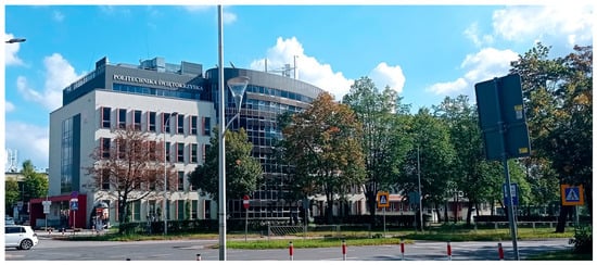
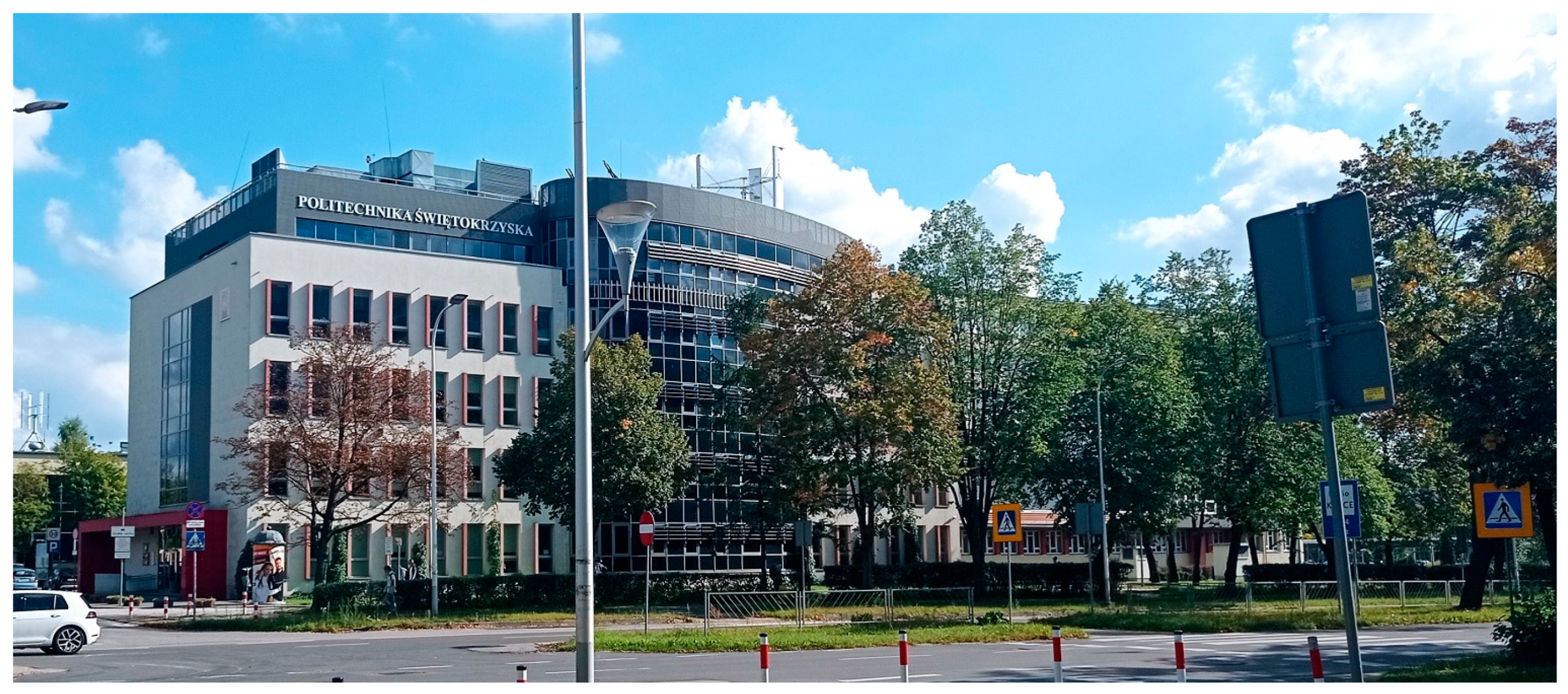
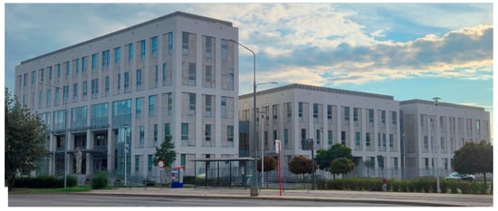
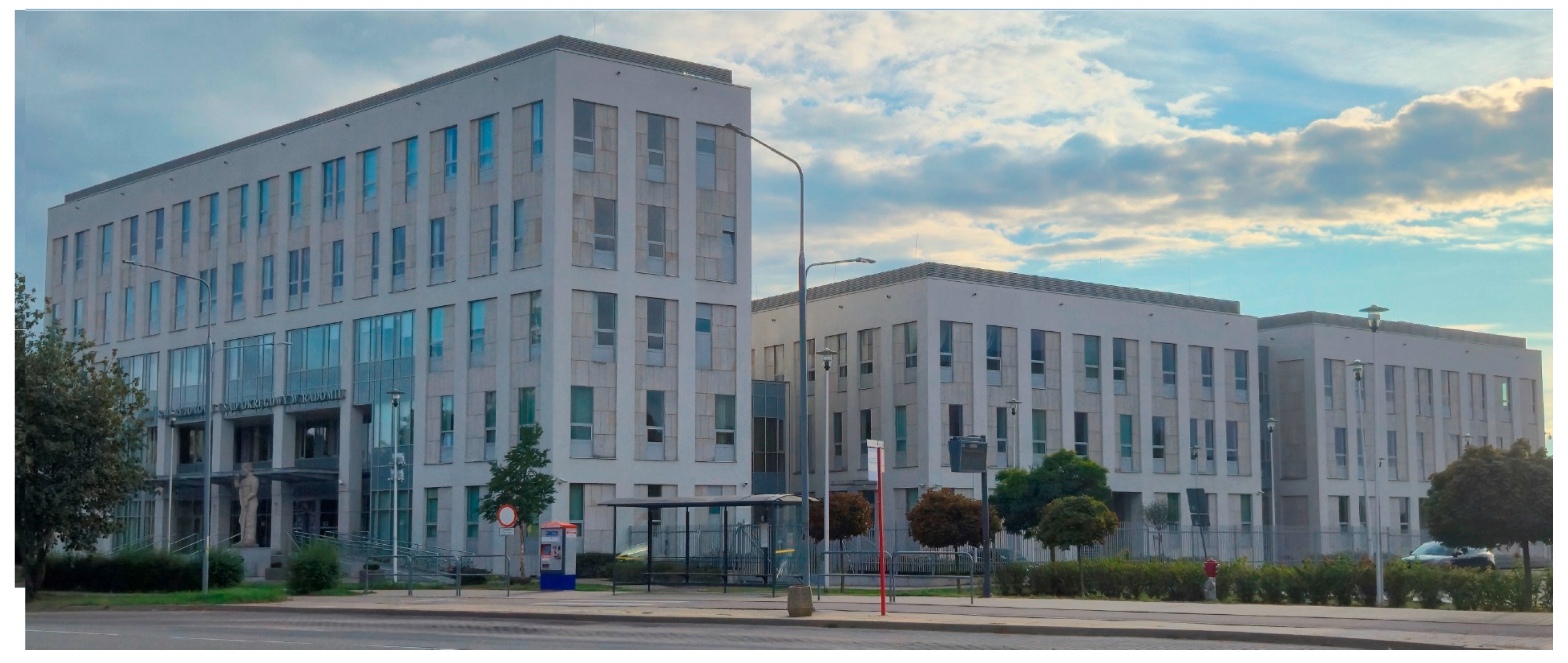
The measurements took place in two intelligent buildings located in two Polish cities: Kielce and Radom (situated about 70 km from one another). The building in Kielce is called “Energis”. It belongs to Kielce University of Technology, and the majority of rooms are lecture rooms and classrooms. It was completed in 2012, and its usable floor area is 5121 m2, while cubature is 21,211 m3. The other one is the courthouse built in 2017, whose usable floor area is 5640 m2, while cubature is 61,661 m3 [57]. Figure 1 and Figure 2 present both buildings.
Figure 1.
“Energis” building of Kielce University of Technology (Western façade).
Figure 2.
Courthouse in Radom (North-East façade).
Both buildings are equipped with the BMS—Building Management System, which manages the building services (includes those mostly responsible for thermal comfort: heating, ventilation, air-conditioning systems). Ventilation ducts (transporting fresh and exhaust air) are placed in the suspended ceilings. Cooling is achieved with the help of fan coils (in the Courthouse) and cassette indoor units (in the “Energis” building). They are connected with the outdoor chillers (situated on the rooftops). Heating in the Courthouse is provided with hot water radiators. In “Energis” both radiators and floor heating systems are used (air heating with the cassette indoor units is also possible). The air temperature in the rooms can be adjusted by room users themselves with control panels placed on the walls in each room. Both buildings are equipped with mechanical ventilation systems with heat recovery units (rotary heat exchangers). The processes occurring in central air handling units (which are located on the rooftops and in the basement of the buildings) consist of filtering, heating, as well as heat recovery. Additionally, steam vaporisers are installed on selected systems. On the courthouse rooftop, chillers operate at the temperature of 7 °C (supply)/12 °C (return), while in “Energis”, the respective values are 6 °C/12 °C. Exhaust air from the toilets is removed with fans, but in “Energis” this air is collected in a special tank in the basement and heat is extracted from it using heat pumps (after this process the air is removed outside). There are 18 separate systems for air supply and removal in the courthouse—with the designed air flowrate ranging from 150 m3/h to 8340 m3/h. In the case of “Energis”, only five with the air flowrate from 2450 m3/h to 21,650 m3/h were designed.
The buildings’ BMS systems control heating, ventilation and air conditioning (HVAC) as well as other structure components (access to rooms, fire prevention monitoring, lighting, etc.). For the present paper, HVAC monitoring was most vital. It is based on controllers that communicate with each other using the LAN network, as well as with modules and a server, using the Modbus technology. It uses shared protocol implemented in each unit. Individual subsystems can be controlled either via local control units installed in specific rooms or centrally from a monitoring and supervision station. Everything is controlled with a central processing unit situated in the buildings and operated by authorised personnel (either onsite or online from a remote location using internet connection).
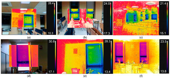
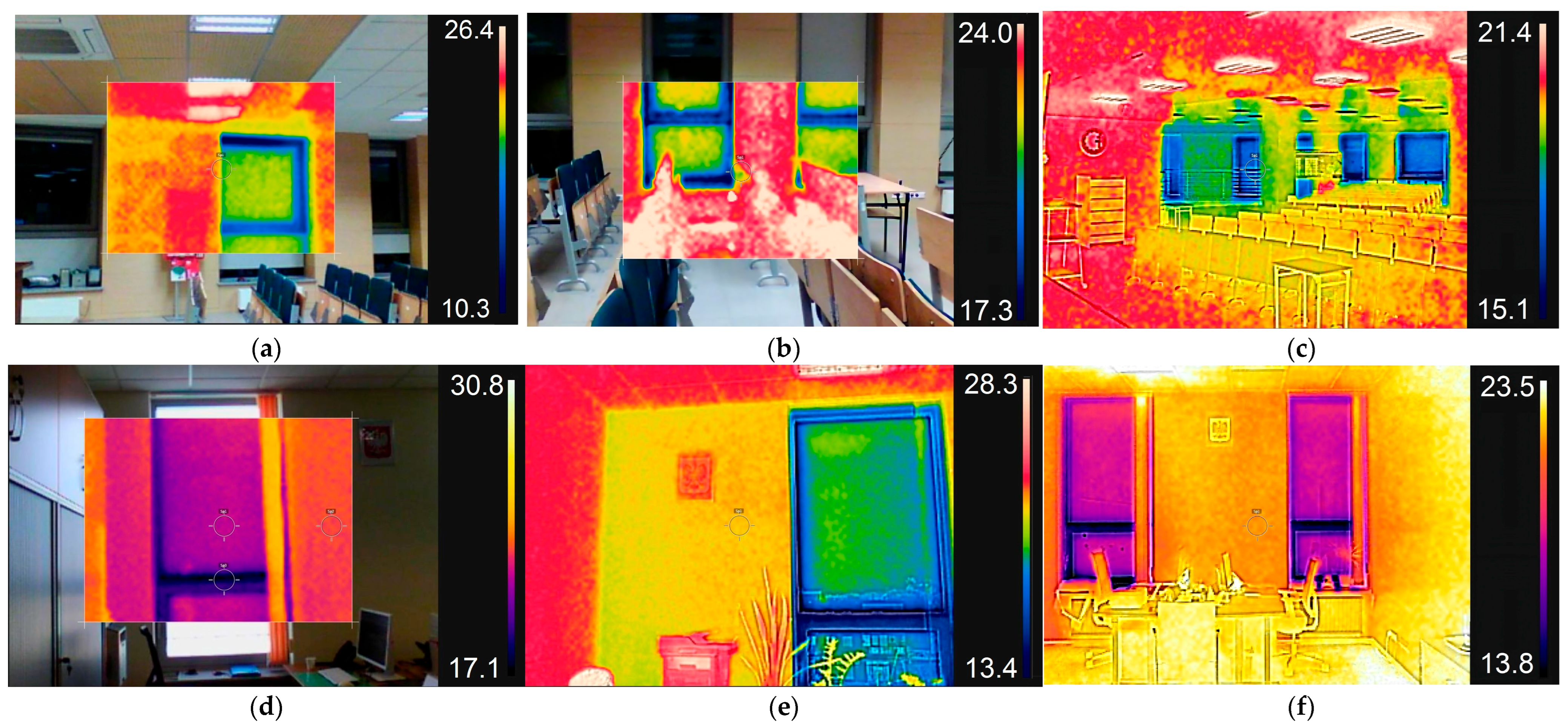
Before thermal comfort testing, infrared measurements were introduced to verify if there are any thermal bridges or other local sources of thermal discomfort in the rooms, which could potentially influence subjective sensations of the respondents. No such problems were detected. Figure 3 presents example thermographic images of the rooms in both buildings.
Figure 3.
Thermographic images of the selected rooms in (a–c) “Energis”; (d–f) the courthouse.
The thermal comfort tests consisted of measuring physical parameters of indoor environment in the selected rooms of the intelligent buildings and completing anonymous questionnaires by the room occupants. The tests usually occurred in the spring (29 tests), slightly fewer in the winter (26) and in the summer (22). They typically took place in the early afternoon: 24 tests between 12.00 and 14.00, 24 between 14.00 and 16.00, 13 between 10.00 and 12.00 and 8 between 8.00 and 10.00 and between 16.00 and 18.00. The largest lecture room was most frequently used (15 times, which corresponds to 19.5% of the tests), followed by a smaller lecture room (10 times). In total, only 12 rooms were used once (located mostly in the courthouse).
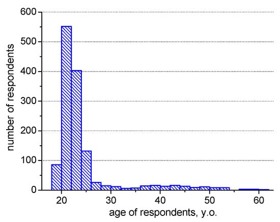
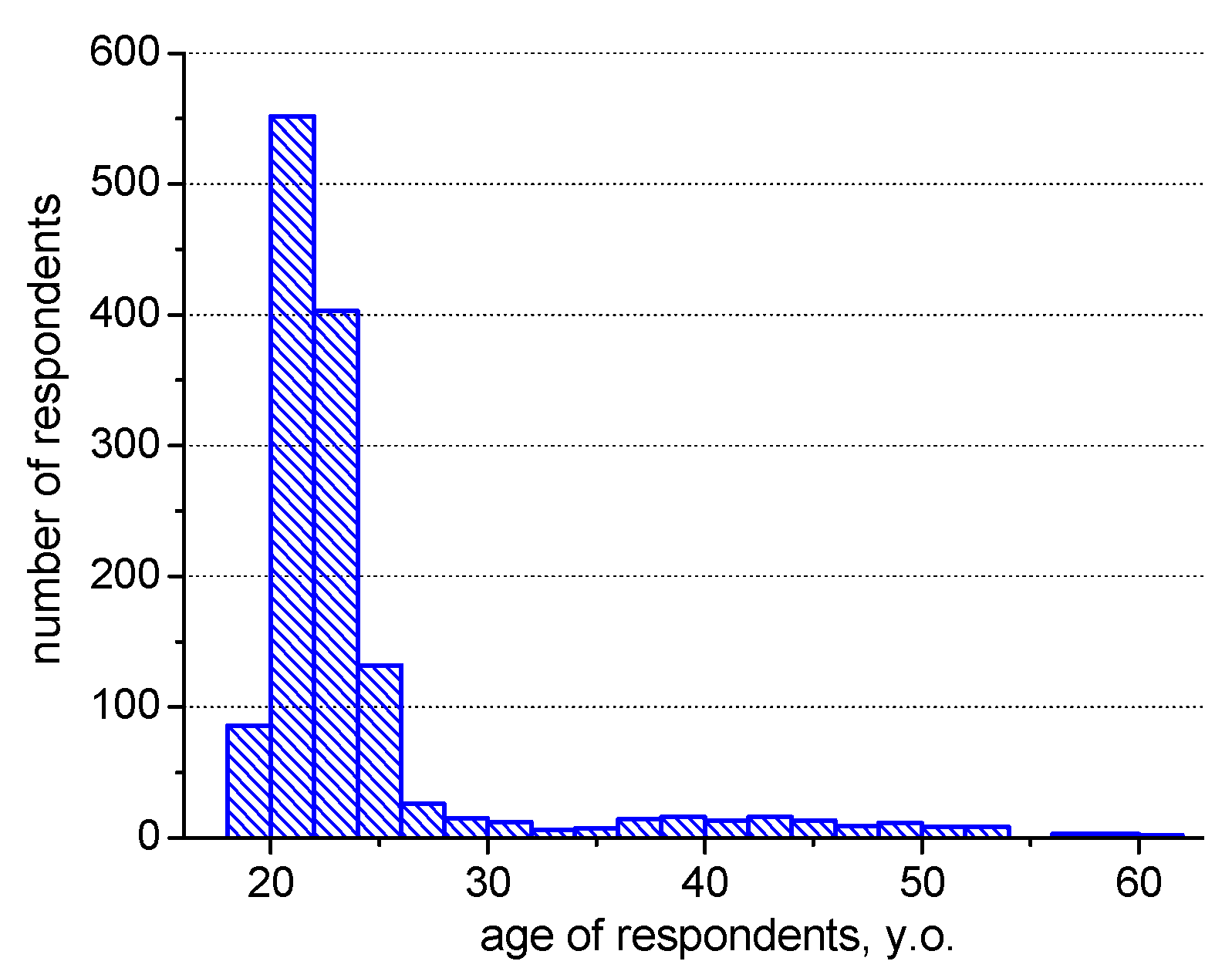
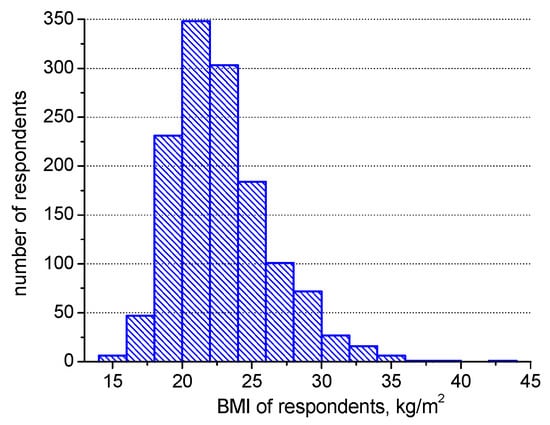
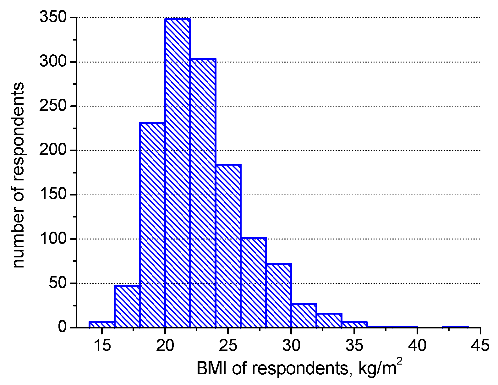
There were between 5 and 65 people in each room. Naturally, fewer people occupied office rooms in the courthouse, while the largest numbers were present in lecture rooms of “Energis” building occupational density ranged from 0.028 to 0.589 people/m2 (the analysis of the impact of occupational density on thermal sensations can be found in the previous paper of the authors [58]). In total, 1369 questionnaire forms were collected. The majority of the respondents were young adults—mostly full-time students in the “Energis” building and medium—aged office workers in the courthouse. The mean value of respondents’ age in “Energis” was 22.0 years old, while the median was 21.0 years old. The respective values in the courthouse were 41.8 and 42.0 years old. Figure 4 presents the histogram with the details. On the other hand, the body mass index (BMI) varied from 15.1 to 43.9 kg/m2 (the median: 22.2 kg/m2). Figure 5 presents histogram of the respondents’ BMI. The share of females and males were 55.7% and 44.3%, respectively.
Figure 4.
The histogram of the respondents’ age.
Figure 5.
The histogram of the respondents’ BMI.
2.2. Testing Equipment and Experimental Method
The experiments consisted in measuring physical parameters of indoor air in the rooms of the buildings (air and globe temperature, air velocity and relative humidity as well as CO2 concentration). Simultaneously, occupants’ subjective sensations regarding indoor environmental conditions were marked on anonymous questionnaires. The collection of the environmental data was performed with BABUC-A microclimate meter (manufacturer: Lsi-Lastem, Dosso - Italy) as well as Sensotron PS32 (manufacturer: Sensotron, Gliwice - Poland). Table 1 provides the basic technical features of the testing system.
Table 1.
Details of the measuring unit.
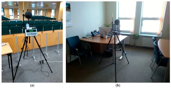
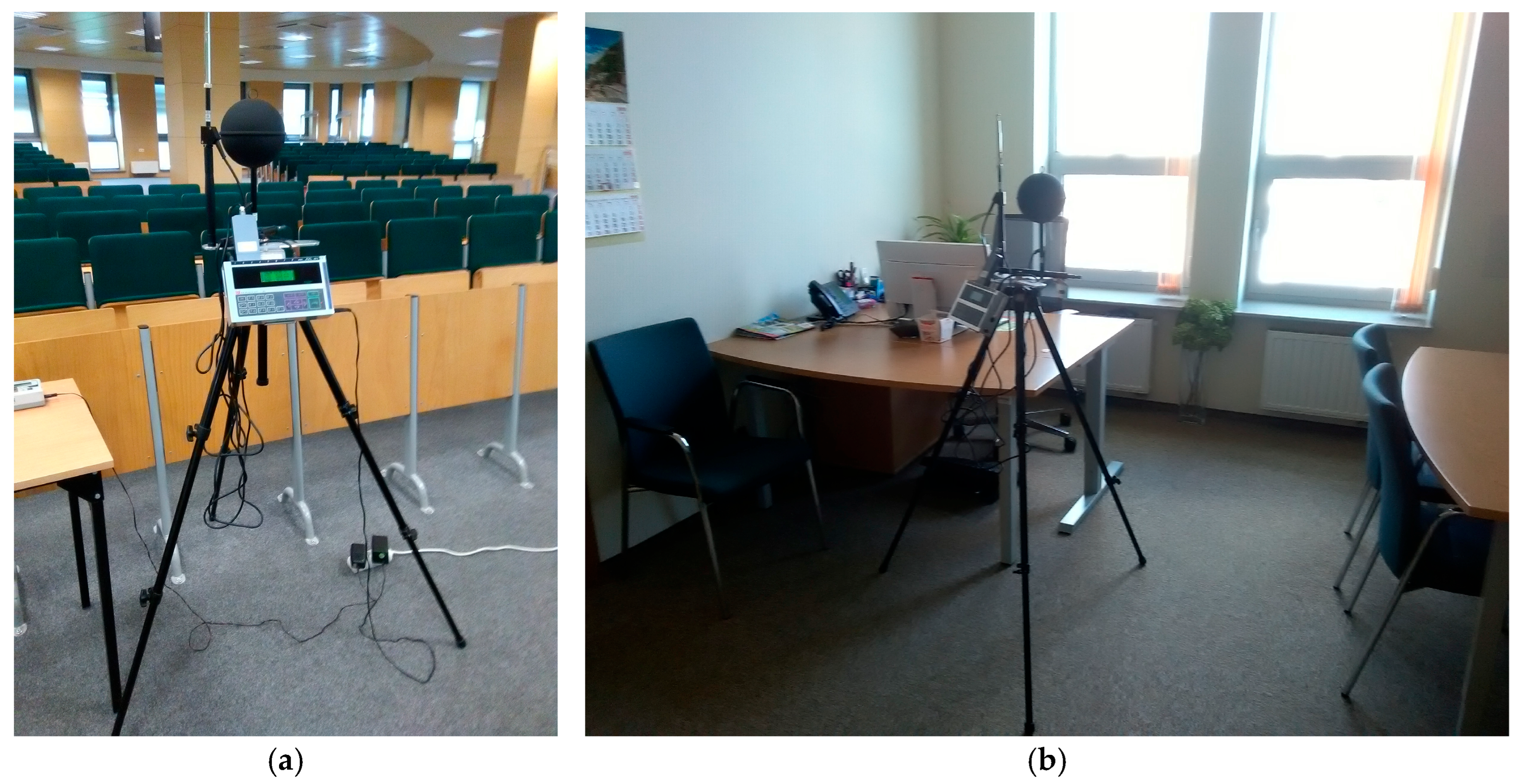
The measuring system was situated at the height of the sitting people as close as possible to the occupants in the rooms. Figure 6 shows the microclimate meter with the probes located on the tripod in example rooms of the intelligent buildings.
Figure 6.
Measuring station in (a) the lecture room of “Energis” building; (b) the office room of the courthouse.
The measurement station was typically located in the middle of the studied group. However, sometimes it was quite challenging (as shown in Figure 6a) because the number of students might be low and they would sit in the first and second row. This made it impossible to place the meter between them (while the assumption of the study was that it should take place under actual conditions). In such rare cases the meter was located not in the middle but as close as possible to the group. During the measurements, the respondents completed a questionnaire form, which also contained additional questions regarding the presence or absence of interfering factors such as heat radiated from the radiators or cold air flow from the windows due to temporarily occurring high winds. If an impact of such additional sources, which could affect the sensations, was detected, the study was repeated (the BMS systems also enabled to temporarily switch off the HVAC systems, which might have generated hot/cold air flow within the rooms).
Data collection took place in 47 different rooms; however—due to the fact that testing occurred several times in some of the rooms—the number of experimental sets was 77 (Table S1 of the Supplementary Materials presents the details of the rooms). The measured indoor environmental parameters were recorded and stored for further processing. At the same time the respondents answered the questions in the anonymous questionnaire forms regarding their subjective sensations. There were 36 questions in the survey; however, only one—regarding thermal sensations—will be considered in the present study. The others have been presented by the authors in the previous studies [57,58]. In the present paper the following question (which the volunteers answered as the first one on the list) was the focus of the analyses: “How do you assess your current thermal sensation”. The possible response to choose by ticking the appropriate box was “too hot” (+3), “too warm” (+2), “pleasantly warm” (+1), “neutral” (0), “pleasantly cool” (−1), “too cool” (−2), “too cold” (−3). The comfort conditions covered the response range from −1 to +1. The values beyond indicated unsatisfactory thermal sensations of the occupants. The experimental results presented in the following section were obtained after 1.2 h of the respondents entering the rooms. The questionnaire forms of the people who performed intense physical activities before the measurements were not considered for the analyses.
2.3. Box–Behnken Method
The method proposed by G.E.P. Box and D.W. Behnken [59] was selected to develop a modification of the thermal comfort model. This method is a class of three-level incomplete factorial designs, which is useful for the estimation of parameters in a second-order polynomial. The methodology places each factor (or independent variable) at one of three equally spaced values, while the design should fit a quadratic model and the ratio of the number of experimental points to the number of coefficients in the quadratic model should be kept at a reasonable level. Moreover, the estimation variance needs to be dependent only on the distance from the centre. At the same time, it should not vary much within the smallest cub with the experimental points.
3. Results and Discussion
3.1. The Impact of Carbon Dioxide Concentration of Thermal Sensations
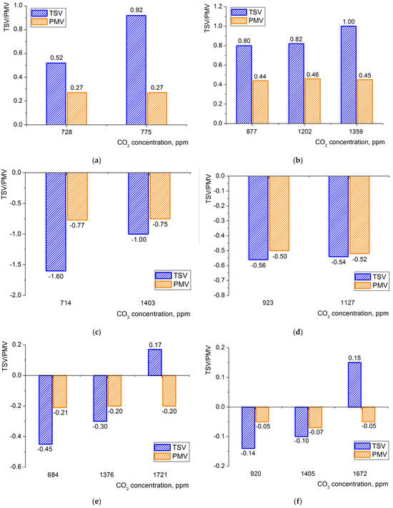
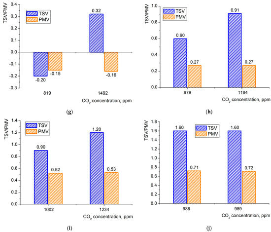
In each of 77 rooms, where the tests took place, the values of indoor environment parameters (including carbon dioxide levels) were measured. The impact of CO2 on thermal comfort, as indicated in the literature review section, is ambiguous because thermal comfort is influenced by many factors. Fanger [8] considered six: air and globe temperature, air velocity, relative humidity as well as clothing thermal insulation and metabolic rate. They are all used in the calculation of PMV values. Thus, in order to determine the impact of carbon dioxide concentration on thermal sensation, several sets containing data from rooms, where the calculated values of PMV were the same, will be considered. The large number of rooms tested (namely, 77) enabled us to find the sets, where PMV values were the same (or differed marginally—by up to 0.2) for 2–3 rooms located either in “Energis” or in the courthouse. However, within each set, different values of the CO2 level were observed in those rooms as well as different values of the subjective thermal sensation vote (TSV) obtained as a mean value marked by the respondents on the questionnaire forms (as presented in Section 2.2). Figure 7 presents the PMV and TSV values in the form of columns, while the x axis represents carbon dioxide concentration in each room. Figure 7a–g represent the results from the “Energis” building, while Figure 7h–j from the courthouse.
Figure 7.
The comparison of subjective TSV values of the respondents in rooms of the same PMV values as a function of CO2 concentration in (a–g) “Energis”; (h–j) the courthouse.
Figure 7a,b show that a rise in the concentration of carbon dioxide was associated with a rise in thermal sensation votes in the selected rooms of the “Energis”—at almost the same positive values of PMV calculated according to the Fanger model. The comparison of the data collected in three rooms (Figure 7b) shows that TSV increased from 0.80 to 1.00, which was accompanied by a rise in the CO2 level—from 877 ppm to 1359 ppm. Figure 7c,d show a similar pattern in the range of negative thermal sensation votes, while Figure 7e–g for the mixed PMV values. The test results obtained in the courthouse (Figure 7h,i) seem to confirm this pattern. At the same time, in two rooms (Figure 7j) PMV was almost identical (+0.71 and +0.72). In both of them, CO2 concentration was also almost the same and amounted to 988–989 ppm. In this case, the subjective assessment of the respondents was the same (TSV = +1.60), too. It further supports the claim that the carbon dioxide level might have an impact on thermal comfort. In order to clarify the impact of carbon dioxide on thermal sensations, the partial Pearson correlation between CO2 and TSV after controlling for PMV (supplemented with multiple linear regression based on the ordinary least squares method—OLS) has been performed covering all the rooms. A two-sided t-test with a significance level of 0.05 was applied. The analysis indicated a weak positive correlation (+0.266), meaning that for comparable PMV values, higher TSV values were related to higher CO2 levels. A 1000 ppm rise in the CO2 concentration was associated with an estimated increase in TSV by 0.2047 points. The p-value was 0.0209, which means that the results are statistically significant. Moreover, a sensitivity analysis based on Heteroskedasticity-Consistent Covariance Matrix Estimator, type 3 (HC3) was applied. It was revealed that after calculating HC3 standard errors the CO2–TSV coefficient remained statistically significant when controlling for PMV with the p value of 0.0406.
3.2. Modified Model Development
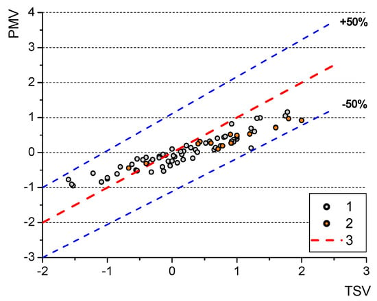
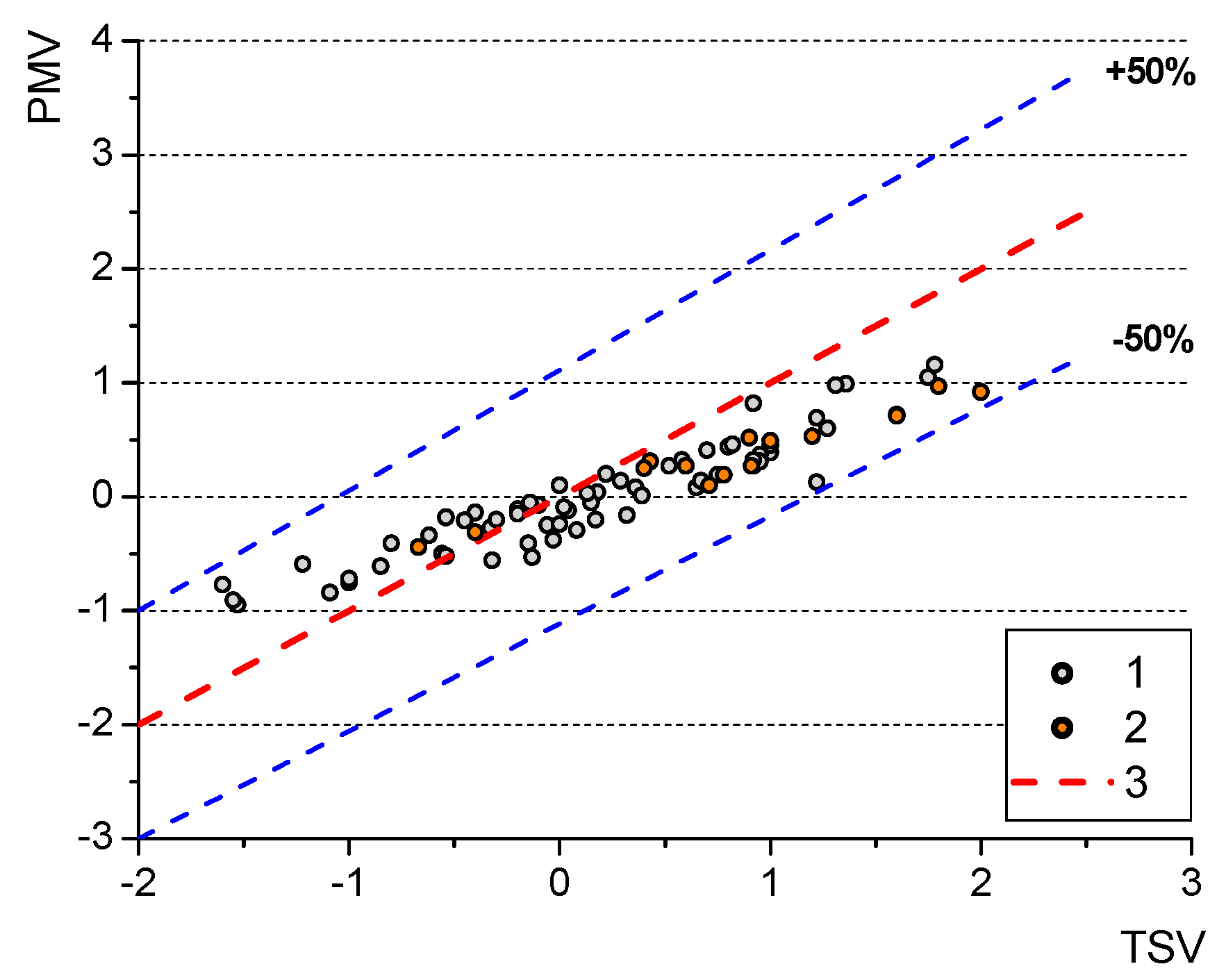
The results presented in Section 3.1 indicate that there might be an impact of carbon dioxide concentration in the analysed rooms of the intelligent buildings regarding thermal sensations of the occupants. At the same time, discrepancies between actual thermal sensations (TSV) expressed by the respondents in anonymous questionnaire forms and the calculated, predicted sensations (PMV) were observed during the analysis of the experimental data. Figure 8 presents the comparison of the actual thermal responses of the occupants of 77 rooms (determined as the mean value from the surveys collected in each room) and the values of PMV calculated according to the Fanger model.
Figure 8.
Comparison between the actual (TSV) and calculated (PMV) thermal sensation responses of the occupants in the “Energis” building (1) and the courthouse (2); dashed red line (3) represents the perfect match of PMV = TSV: dashed blue lines represent ±50% agreement bands.
As can be seen, the model does not predict actual thermal sensations of the respondents very precisely; the deviation from the perfect match line is within ±50% (both buildings showed a similar pattern). As indicated earlier, in many previous studies the model either overpredicted or underpredicted the actual thermal sensations. However, in the present study focused on intelligent buildings, the model seems to overpredict thermal sensations in “colder” environments and underpredict them in “warmer” environments (the turning point is exactly 0.0). In order to improve the model, a modification will be developed based on the application of the Box–Behnken method and the introduction of a new parameter into the model, namely the CO2 concentration.
The original equation for PMV is as follows [9]:
where M is metabolic rate, W/m2; W—effective mechanical power, W/m2; fcl—clothing surface area factor; pa—water vapour partial pressure, Pa; hc—convective heat transfer coefficient, W/(m2K); ta—indoor air temperature, °C; tcl—clothing surface temperature, °C; tr—mean radiant temperature, °C.
The above equation will be modified using a four-factor Box–Behnken analysis, involving 27 combinations of coded variable levels. The constants in Equation (1) were marked as X and equal: X1 = 0.303, X2 = −0.036, X3 = 0.028. Table 2 presents the estimated maximal range within which the constants can vary. Moreover, a new constant X4 (representing the impact of CO2 concentration) was introduced there together with the estimated range. The values were obtained through mathematical analysis of their impact on the PVM values with the assumption that the boundary values had to have significant impact on the final result).
Table 2.
The range of the variation in the parameters.
A combination of the above-mentioned values will be tested to obtain the highest precision of PMV determination. Table 3 presents the test program in terms of coded variable levels for the four parameters of the modified PMV model (the left column) as well as the actual variable levels for these four parameters (the right column).
Table 3.
Variable levels of the parameters.
There were 77 separate tests conducted in the rooms of the intelligent buildings. They were further divided into 19 sets, which grouped the rooms which were similar in nature (in terms of the same testing time: spring, summer, autumn, winter and certain indoor air temperature ranges). For those 19 sets (groups of rooms) the calculations based on the RSM (Response Surface Methodology) procedure were conducted. It was found that the values of all four constants significantly impacted the final result of the PMV calculation. For each set, the values of four constants were determined, which best fitted the actual results. Afterwards, the values obtained in each set were validated against data collected in 77 rooms. Thus, 77 × 19 = 1493 values of PMV were determined and compared with the actual thermal sensations. The highest accuracy set (set numbered “11”) was found this way. The SAS software (version 9.3) developed by SAS Institute Inc., Cary, NC, USA was applied in the analyses; the details are presented in the Supplementary Material. The response surface model for the variable set-11 fits the data very well (R2 = 0.9990) and is highly statistically significant (F = 901.28; p < 0.0001). All four analysed factors (constant1, constant 2, constant 3, and constant4) show a considerable influence on the variable under study (p < 0.0001) (Table S2 of the Supplementary Materials). The linear component of the model contributes most to explaining the response variability, accounting for 97.87% of the variation. Quadratic terms and interactions between factors are also significant. The lack-of-fit test revealed no significant differences between the model and the observed data (F = 1.31; p = 0.5081), confirming a good model fit. Table S3 of the Supplementary Materials provides data on the RSREG procedure regarding the final values of the constants, which were obtained for the coded radius of 1 as the optimal solution. Those values are: X1 = 0.475, X2 = −0.033, X3 = 0.040 and X4 = 0.000018. Thus, the modified equation (based on the original model [9]) takes the following form:
where C is the carbon dioxide level in ppm.
In order to determine the relationship between the TSV value obtained from the survey and the PMV value, a linear regression analysis was conducted using the SAS REG procedure. The analysis was performed on 77 observations. The resulting model proved to be statistically significant (F = 653.55; p < 0.0001) and demonstrated a very good fit to the data. The coefficient of determination was R2 = 0.8971, while the adjusted coefficient of determination was R2 = 0.8957. This indicates that approximately 89.71% of the variation in the PMV values was explained by the variation in the TSV values. The estimated regression equation took the form PMV = −0.20543 + 1.13072·TSV. The regression coefficient for the TSV variable was positive and statistically significant (t = 25.56; p < 0.0001), indicating a strong, positive relationship between the analysed PMV values. The results indicate a very good fit for the linear regression model and a significant relationship between TSV and the calculated PMV values. Table S4 in the Supplementary Materials provides the details.
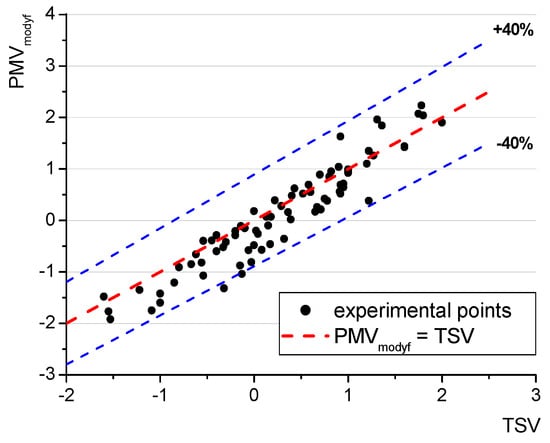
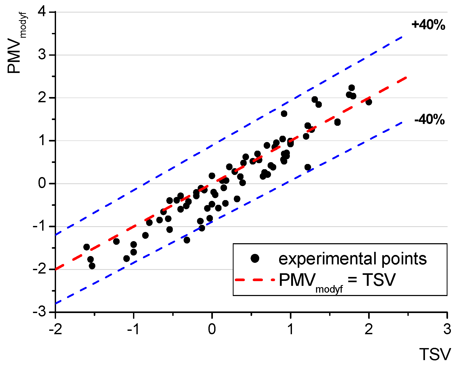
A comparison of the PVM values determined according to the modified Equation (2) with the actual thermal sensation votes (TSV) according to the questionnaire study has been presented in Figure 9. Almost all of the experimental points are situated within ±40% error band (as opposed to ±50% in the case of the original model).
Figure 9.
The comparison between the actual (TSV) and calculated (PMVmodyf) thermal sensation responses of the occupants; dashed red line represents the perfect match: dashed blue lines represent ±40% agreement bands.
The modified equation was characterised by lower mean absolute error MAE (of 0.293) than the original equation (0.385). Root mean square errors (RMSEs) were also smaller in the case of the modified formula (0.378) than the original one (0.460). A paired-sample t-test comparing absolute prediction errors indicated a statistically significant reduction in MAE (p = 0.0199). The additional results of the statistical analysis of the models’ performance carried out at the confidence level of 0.05 have been presented in Table S5 in the Supplementary Materials.
However, the question arises if the enhancement in the prediction potential of the modified equation is attributed to the values of new constants or the impact of the CO2 component. The response surface analysis (carried out in SAS software using the RSREG procedure) indicated that the specified discrepancy function could be reduced by jointly varying the four constants. Table S3 and Figure S1 (both of the Supplementary Materials) present the details of the analyses for set “11”. Along the minimum response ridge, the estimated response decreased from 0.140674 to 0.066982, while the impact of all four constants was observed, although it seems to be lowest for the fourth one (Figure S1). In the response surface model, the linear coefficient for Constant4 (related to the CO2 level) was statistically significant (t = −2.34; p = 0.0373). This fact indicates that the variation in the coefficient associated with CO2 was related to the variation in the objective function within the analysed region. On the other hand, a comparison of the modified PMV equation with and without the CO2 component (but with new values of the other three constants) shows that there is no statistically significant difference between the results generated by the two modified equations based on the dataset considered in the analyses.
The thermal comfort model proposed by Fanger [8] also enables us to determine the expected percentage of people who are dissatisfied with the indoor environmental conditions prevailing in a certain room, namely the PPD index. A modification of this index has also been conducted, which consisted of determining new values of two constants in the equation for PPD. In the original formula they equal −0.03353 and −0.2179 [9], while the modified equation (originating from Ref. [9]) takes the following form:
PPD = 100 − 95 ⋅ exp(0.0408PMV4 − 0.5067PMV2),
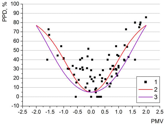
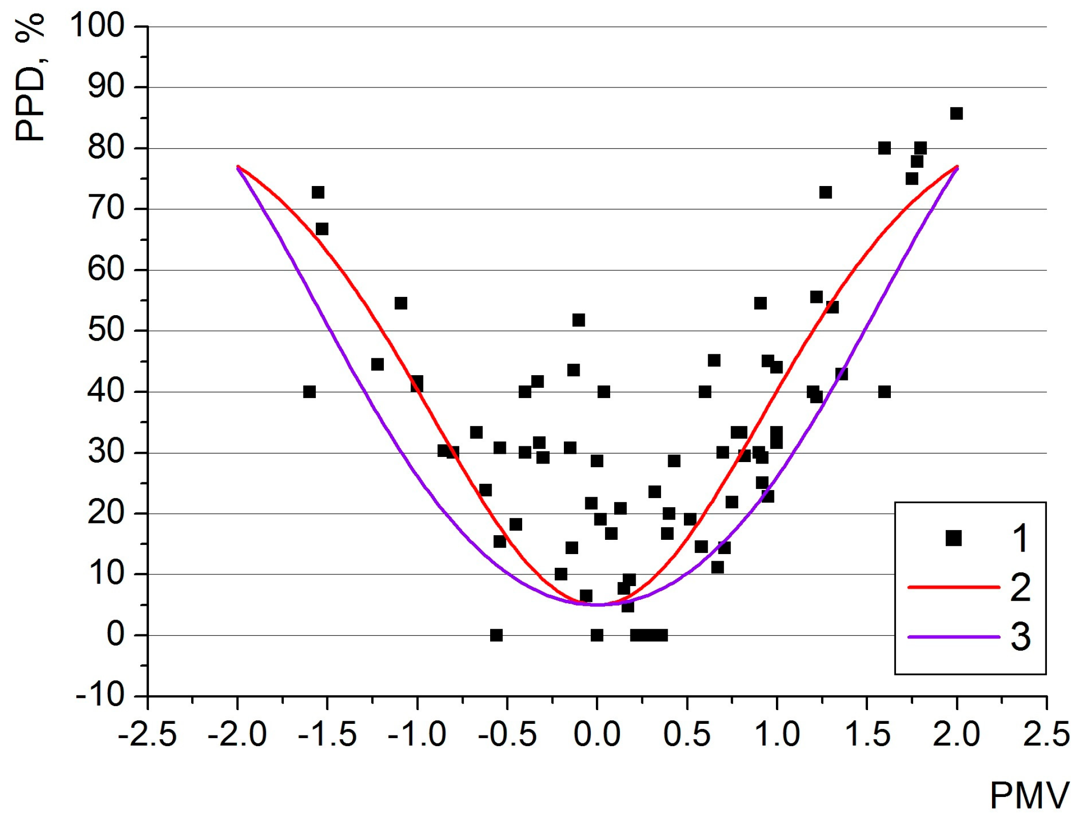
Figure 10 presents the comparison of the actual values of PPD as reported by the respondents in the study conducted in 77 rooms of the intelligent buildings. It was calculated as a share of the occupants’ “negative” responses to the question regarding their thermal sensations (namely, the total share of responses “+3”, “+2”, “−2” and “−3”). The respondents who marked whose answers in the questionnaire forms felt either too warm or too cold and were beyond their thermal comfort range.
Figure 10.
The experimental results of the PPD index in 77 rooms (1) together with the calculation results according to the original PPD Equation (2) determined with [9] and the modified PPD Equation (3).
Similarly to the results of the statistical analyses of PMV discussed earlier, in the case of PPD the modified equation proved to be more accurate than the original one. The mean absolute error of the original PPD equation was 23.32, while of the modified equation was 19.13 (17.9% reduction), while the root mean square errors were reduced by 17.1% (from 27.77 in the case of the original equation to 23.02 in the case of the modified equation). The improvement proved to be statistically significant based on a two-sided paired t-test applied to the differences between the absolute errors. Table S6 of the Supplementary Materials provides additional data.
It needs to be noted that Equation (3) has significant limitations. During its development, each measurement session received equal weight, irrespective of the number of respondents, and no sign constraints were imposed. The produced formula should rather be considered as a local empirical fit over the observed experimental values of the present study rather than as a generally valid PPD model.
Both the modified equations (PMV and PPD) have been developed based on the experimental dataset covering 1369 questionnaire forms collected in 77 rooms, and thus, they can be limited in their application potential. The respondents are mainly young adults in their twenties, while the measurements took place in two intelligent buildings in Poland (in the temperate transitional climate). The validity of the developed equations is also limited to the values of carbon dioxide concentration (of 550–1996 ppm) recorded during the tests.
3.3. Energy Consumption Implications Related to the Modified Thermal Comfort Model
As can be seen in Figure 7, there is quite a large discrepancy between the calculations of thermal sensations according to the original model and the actual sensations of the respondents. The modified PMV equation provides more accurate results and consequently provides better guidelines for setting heating, ventilation and air-conditioning systems in the buildings (which could use energy for air treatment processes more efficiently). It is a substantial advantage because thermal comfort conditions could be obtained. This is especially important in educational or office buildings due to the fact that productivity related to either learning or working activities would also be improved, which is an additional benefit.
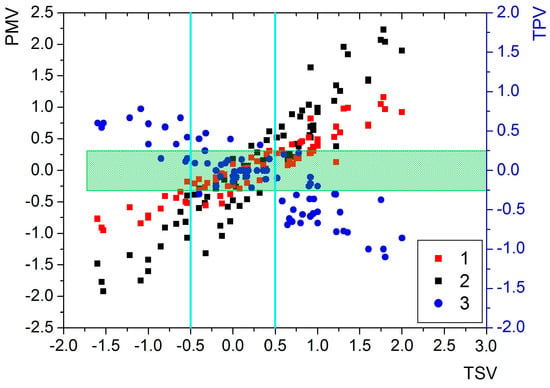
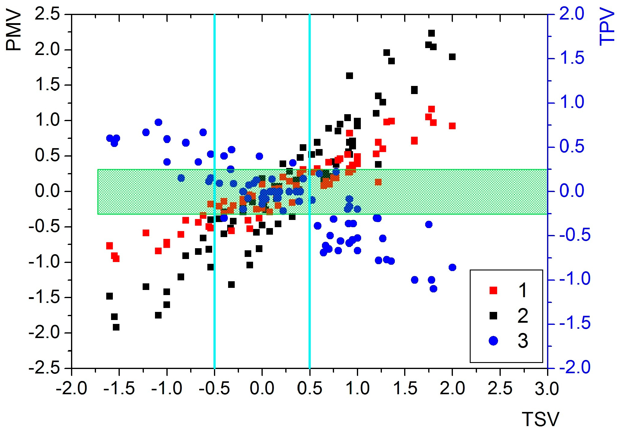
From the energy consumption point of view, the issue is more complex. In the previous study of the authors [57], data regarding the occupants’ thermal preferences was presented. The study participants located in 77 rooms responded to the following issue in the questionnaire form: “I would like in this room to be: “much warmer” (+2), “warmer” (+1), “no change” (0), “cooler” (−1), “much cooler” (−2). This is expressed as TPV—thermal preference vote. Figure 11 presents the relation between the average TPV values marked in the questionnaire forms collected in the room vs. average TSV values expressed by the occupants in each of the room (3). The same figure contains data of the PMV values calculated with the original and modified formula.
Figure 11.
The relation between the actual (TSV) and calculated (PMV) thermal sensation values according to the original model (1) and the modified model (2) as well as thermal preference vote (TPV) (3)—data according to Ref. [57]; the green rectangle represents the area of −0.25 < TPV < +0.25, and the solid cyan lines represent the values of TSV: −0.5 and +0.5.
Naturally, if the respondents felt too hot/warm they would like it to be cooler (and marked lower values of TPV), while if they were cold, they would prefer to increase the air temperature (marking positive TPV values). If thermal satisfaction was experienced, no change (TPV = 0) would be anticipated. The green area between −0.25 < TPV < +0.25 represents highly acceptable thermal conditions, under which the occupants felt no need for temperature change. If the respondents in the rooms felt cold (TSV < −0.5), they would like the air temperature to rise. This occurred in 11 rooms (Figure 11 on the left to the line TSV = −0.5). According to the original model, thermal sensation (PMV) values below −0.5 were observed in 12 rooms and slightly more in the case of conducting calculations according to the modified model. If such settings were used in the HVAC system, heating would be initiated in those rooms. On the other hand, at higher temperatures people opted for temperature reduction. This phenomenon was observed in 27 rooms (Figure 11). However, the calculations carried out with the original model indicate that only 19 rooms might require temperature reduction. The modified model provided more accurate assessment, according to which air temperature might be reduced in 29 rooms. Theoretically, the original model leads to less energy consumption because heating and cooling occurs more rarely than in the case of the modified model—if they are used for HVAC systems’ settings. However, a closer look provides a different picture. Namely, if the respondents are dissatisfied with the indoor conditions, they adjust the indoor air temperature themselves using control panels in the rooms. Typically, they overexaggerate the need to either increase or decrease temperature, which leads to overheating in winter and overcooling in summer. After a while, in the first case (winter conditions), windows might be open to cool down the rooms, which leads to energy loss. In the second case of summer conditions (which is even more important because the cost of providing cooling is about three times higher than the cost of providing heating in these two intelligent buildings), temperature reduction could be too high, and thermal comfort could be severely disrupted. This might also lead to opening windows or switching to the heating mode operation of the HVAC system, which would increase the energy consumption even further.
4. Conclusions
The paper provided new insights into two important areas of thermal comfort studies, namely the impact of carbon dioxide concentration and the development of a modified thermal comfort model together with a discussion of the energy consumption implications. The following conclusions can be drawn:
- Based on the observations carried out in the selected rooms of the analysed intelligent buildings a rise in the concentration of carbon dioxide was associated with a rise in thermal sensation votes (however, the number of compared cases was relatively low). The partial Pearson correlation between CO2 and TSV after controlling for PMV indicated a weak positive correlation, meaning that for comparable PMV values, higher TSV values were related to higher CO2 levels. A 1000 ppm rise in the CO2 concentration was associated with an estimated increase of TSV by 0.2047 points.
- The original thermal comfort model did not prove to be very accurate when validated against a large dataset of 1369 questionnaire forms collected in two intelligent buildings. The differences between the actual and calculated thermal sensations were up to 50% and were not aligned with the ideal prediction line of PMV = TSV, indicating that there might be a problem related to the application of the original Fanger model to intelligent buildings. Both buildings showed the same pattern of data spread; however, thermal environment in the courthouse was typically warmer, and thus, positive TSV values were more common there.
- The modification of the PMV equation was based on the Box–Behnken concept, which has not been found in the literature so far. The modified equation provided more accurate results in relation to the original model; the spread of the experimental data was reduced to ca. 40%, and the results are situated along the PMV = TSV ideal prediction line. The modified formula was characterised by lower mean absolute error (of 0.293) than the original equation (0.385) and lower root mean square errors: 0.378 and 0.460, respectively.
- The modified equation for the predicted percentage of the dissatisfied (PPD) was developed based on the same large experimental dataset collected in the intelligent buildings and provided higher accuracy than the original PPD equation (mean absolute and root mean square errors were reduced by over 17%).
- The influence of the modified thermal comfort model with regard to energy consumption seems to be complicated. Theoretically, if the heating, ventilation and air-conditioning systems’ setting are based on the original model, lower energy consumption might be anticipated. However, in this case the occupants might take “adjusting actions” themselves (setting air temperature on their own in the rooms), which would be quite unfavourable regarding energy consumption. At the same time, the additional advantage of the modified model is that it might provide better indoor environment conditions. This would lead to improved productivity in office buildings and better knowledge acquisition in educational buildings.
Supplementary Materials
The following supporting information can be downloaded at https://www.mdpi.com/article/10.3390/en19215276/s1, Table S1: Data of rooms where the tests took place; Table S2: Calculation results performed in the SAS software for set-11 according to the RSREG procedure; Table S3: Values of the four factors leading to minimum and maximum values; Table S4: Regression analysis results regarding the dependence of PMV on the constants; Table S5: PMV determination accuracy assessment; Table S6: PPD determination accuracy assessment; Figure S1: Ridge analysis of the response surface performed using the SAS RSREG procedure.
Author Contributions
Conceptualisation, Ł.J.O. and G.M.; methodology, Ł.J.O., G.M. and M.T.; software, Ł.J.O. and N.R.; validation, Ł.J.O., G.M., S.H. and N.R.; formal analysis, Ł.J.O., G.M. and S.H.; investigation, G.M.; resources, Ł.J.O., S.H., N.R. and M.T.; data curation, G.M.; writing—original draft preparation, Ł.J.O., G.M. and S.H.; writing—review and editing, Ł.J.O., G.M., S.H. and N.R.; supervision, Ł.J.O. and M.T.; project administration, Ł.J.O. and S.H., funding acquisition, S.H. All authors have read and agreed to the published version of the manuscript.
Funding
The work in the paper was supported by the project “REFRESH—Research Excellence For REgion Sustainability and High-tech Industries”, (VP2), (Reg. No.: CZ.10.03.01/00/22_003/0000048) co-funded by the European Union.
Data Availability Statement
Data available from the corresponding author upon request.
Conflicts of Interest
The authors declare no conflicts of interest.
Abbreviations
The following abbreviations are used in this manuscript:
| CO2 | Carbon dioxide |
| PMV | Predicted Mean Vote |
| PPD | Predicted Percentage Dissatisfied |
| TPV | Thermal preference vote |
| TSV | Thermal sensation vote |
References
- International Energy Agency. Energy Technology Perspectives 2026; International Energy Agency: Paris, France, 2026. [Google Scholar]
- Moujalled, B.; Cantin, R.; Guarracino, G. Comparison of thermal comfort algorithms in naturally ventilated office buildings. Energy Build. 2008, 40, 2215–2223. [Google Scholar] [CrossRef] [Scilit]
- Merabtine, A.; Maalouf, C.; Waheed Hawila, A.A.; Martaj, N.; Polidori, G. Building energy audit, thermal comfort, and IAQ assessment of a school building: A case study. Build. Environ. 2018, 145, 62–76. [Google Scholar] [CrossRef] [Scilit]
- Yang, W.; Zhang, G. Thermal comfort in naturally ventilated and air-conditioned buildings in humid subtropical climate zone in China. Int. J. Biometeorol. 2008, 52, 385–398. [Google Scholar] [CrossRef] [Scilit]
- Hong, S.H.; Lee, J.M.; Moon, J.W.; Lee, K.H. Thermal comfort. energy and cost impacts of PMV control considering individual metabolic rate variations in residential building. Energies 2018, 11, 1767. [Google Scholar] [CrossRef] [Scilit]
- Robledo-Fava, R.; Hernández-Luna, M.C.; Fernández-de-Córdoba, P.; Michinel, H.; Zaragoza, S.; Castillo-Guzman, A.; Selvas-Aguilar, R. Analysis of the influence subjective human parameters in the calculation of thermal comfort and energy consumption of buildings. Energies 2019, 12, 1531. [Google Scholar] [CrossRef] [Scilit]
- Albatayneh, A.; Alterman, D.; Page, A.; Moghtaderi, B. The Impact of the Thermal Comfort Models on the Prediction of Building Energy Consumption. Sustainability 2018, 10, 3609. [Google Scholar] [CrossRef] [Scilit]
- Fanger, P.O. Calculation of thermal comfort: Introduction of a basic comfort equation. ASHRAE Trans. 1967, 73, III4.1–III4.20. [Google Scholar]
- ISO Standard 7730; Ergonomics of the Thermal Environment—Analytical Determination and Interpretation of Thermal Comfort Using Calculation of the PMV and PPD Indices and Local Thermal Comfort Criteria. International Organization for Standardization: Geneva, Switzerland, 2005.
- ANSI/ASHRAE Standard 55-2017; Thermal Environmental Conditions for Human Occupancy. American Society of Heating. Refrigerating and Air-Conditioning Engineering: Peachtree Corners, GA, USA, 2017.
- EN 16798-1:2019; Energy Performance of Buildings—Ventilation for Buildings—Part 1: Indoor Environmental Input Parameters for Design and Assessment of Energy Performance of Buildings Addressing Indoor Air Quality, Thermal Environment, Lighting and Acoustics—Module M1-6. European Committee for Standardisation: Brussels, Belgium, 2019.
- Ricciardi, P.; Buratti, C. Environmental quality of university classrooms: Subjective and objective evaluation of the thermal, acoustic, and lighting comfort conditions. Build. Environ. 2018, 127, 23–36. [Google Scholar] [CrossRef] [Scilit]
- Aghniaey, S.; Lawrence, T.W.; Sharpton, T.N.; Douglass, S.P.; Oliver, T.; Sutter, M. Thermal comfort evaluation in campus classrooms during room temperature adjustment corresponding to demand response. Build. Environ. 2019, 148, 488–497. [Google Scholar] [CrossRef] [Scilit]
- Hens, H.S.L.C. Thermal comfort in office buildings: Two case studies commented. Build. Environ. 2009, 44, 1399–1408. [Google Scholar] [CrossRef] [Scilit]
- Kuchen, E.; Fisch, M.N. Spot Monitoring: Thermal comfort evaluation in 25 office buildings in winter. Build. Environ. 2009, 44, 839–847. [Google Scholar] [CrossRef] [Scilit]
- Ricciardi, P.; Buratti, C. Thermal comfort in open plan offices in northern Italy: An adaptive approach. Build. Environ. 2012, 56, 314–320. [Google Scholar] [CrossRef] [Scilit]
- Indraganti, M.; Ooka, R.; Rijal, H.B. Thermal comfort in offces in summer: Findings from a field study under the ‘setsuden’ conditions in Tokyo. Japan. Build. Environ. 2013, 61, 114–132. [Google Scholar] [CrossRef] [Scilit]
- Obi-George, L.C.; Ifebi, O.C.; Nwokorie, A.J.; Maduka, N.M.; Ibe, P.C.; Okoro, O.N.; Iweha, C.M. Thermal comfort in residential buildings: A case for building material efficiency on occupants wellbeing. Int. J. Innov. Environ. Stud. Res. 2024, 12, 174–197. [Google Scholar]
- Sadłowska-Sałęga, A.; Burda, W.; Moskal, K. Perception of Environmental Comfort in Historic Museum Buildings Depending on the Method of Active Microclimate Control—A Case Study of the National Museum in Krakow. Energies 2026, 19, 170. [Google Scholar] [CrossRef] [Scilit]
- Khatoon, S.; Shah, A.N. Prediction of Comfort Parameters for Naturally Ventilated Underground Car Parks. Nucleus 2016, 3, 214–220. [Google Scholar] [CrossRef] [Scilit]
- Khatoon, S.; Kim, M.-H. Human Thermal Comfort and Heat Removal Efficiency for Ventilation Variants in Passenger Cars. Energies 2017, 10, 1710. [Google Scholar] [CrossRef] [Scilit]
- Atmaca, A.B.; Zorer Gedik, G. Development of energy efficient design proposals for air conditioned mosques: Temperate humid climate case. Heliyon 2023, 9, e20992. [Google Scholar] [CrossRef] [Scilit]
- Yang, L.; Yan, H.; Lam, J.C. Thermal comfort and building energy consumption implications—A review. Appl. Energy 2014, 115, 164–173. [Google Scholar] [CrossRef] [Scilit]
- Arowoiya, V.A.; Onososen, A.O.; Moehler, R.C.; Fang, Y. Influence of Thermal Comfort on Energy Consumption for Building Occupants: The Current State of the Art. Buildings 2024, 14, 1310. [Google Scholar] [CrossRef] [Scilit]
- Fedorczak-Cisak, M.; Kowalska-Koczwara, A.; Buda-Chowaniec, A.; Dechnik, M.; Ciuła, M.; Shymanska, A. Fan Coil Unit Influence on Thermal Comfort in Waiting Areas of Energy-Efficient Office Buildings. Energies 2025, 18, 6187. [Google Scholar] [CrossRef] [Scilit]
- Becker, R.; Paciuk, M. Thermal comfort in residential buildings—Failure to predict be Standard model. Build. Environ. 2009, 44, 948–960. [Google Scholar] [CrossRef] [Scilit]
- Mors, S.T.; Hensen, J.L.M.; Loomans, M.G.L.C.; Boerstra, A.C. Adaptive thermal comfort in primary school classrooms: Creating and validating PMV-based comfort charts. Build. Environ. 2011, 46, 2454–2461. [Google Scholar] [CrossRef] [Scilit]
- Indraganti, M.; Ooka, R.; Rijal, H.B. Field investigation of comfort temperature in Indian office buildings: A case of Chennai and Hyderabad. Build. Environ. 2013, 65, 195–214. [Google Scholar] [CrossRef] [Scilit]
- Manu, S.; Shukla, Y.; Rawal, R.; Thomas, L.E.; de Dear, R. Field study of thermal comfort cross multiple climate Jones for the subcontinent: India Model for Adaptive Comfort (IMAC). Build. Environ. 2016, 98, 55–70. [Google Scholar] [CrossRef] [Scilit]
- Vilcekova, S.; Meciarova, L.; Burdova, E.K.; Katunska, J.; Kosicanova, D.; Doroudiani, S. Indoor environmental quality of classrooms and occupants’ comfort in a special education school in Slovak Republic. Build. Environ. 2017, 120, 29–40. [Google Scholar] [CrossRef] [Scilit]
- Balbis-Morejón, M.; Rey-Hernández, J.M.; Amaris-Castilla, C.; Velasco-Gómez, E.; San José-Alonso, J.F.; Rey-Martínez, F.J. Experimental Study and Analysis of Thermal Comfort in a University Campus Building in Tropical Climate. Sustainability 2020, 12, 8886. [Google Scholar] [CrossRef] [Scilit]
- Campano, M.Á.; Domínguez-Amarillo, S.; Fernández-Agüera, J.; Sendra, J.J. Thermal Perception in Mild Climate: Adaptive Thermal Models for Schools. Sustainability 2019, 11, 3948. [Google Scholar] [CrossRef] [Scilit]
- Gong, X.; Meng, Q.; Yu, Y. A Field Study on Thermal Comfort in Multi-Storey Residential Buildings in the Karst Area of Guilin. Sustainability 2021, 13, 12764. [Google Scholar] [CrossRef] [Scilit]
- Alonso, A.; Suárez, R.; Llanos-Jiménez, J.; Muñoz-González, C.M. Students’ thermal and indoor air quality perception in secondary schools in a Mediterranean climate. Energy Build. 2025, 333, 115479. [Google Scholar] [CrossRef] [Scilit]
- Cheung, T.; Schiavon, S.; Parkinson, T.; Li, P.; Brager, G. Analysis of the accuracy on PMV–PPD model using the ASHRAE Global Thermal Comfort Database II. Build. Environ. 2019, 153, 205–217. [Google Scholar] [CrossRef] [Scilit]
- Staveckis, A.; Borodinecs, A. Impact of Temperature Drift on Thermal Sensation in nZEB Residential Buildings Under Winter Conditions. Energies 2026, 19, 151. [Google Scholar] [CrossRef] [Scilit]
- Piasecki, M.; Fedorczak-Cisak, M.; Furtak, M.; Biskupski, J. Experimental Confirmation of the Reliability of Fanger’s Thermal Comfort Model—Case Study of a Near-Zero Energy Building (NZEB) office Building. Sustainability 2019, 11, 2461. [Google Scholar] [CrossRef] [Scilit]
- Omidvar, A.; Jungsoo Kim, J. Modification of sweat evaporative heat loss in the PMV/PPD model to improve thermal comfort prediction in warm climates. Build. Environ. 2020, 176, 106868. [Google Scholar] [CrossRef] [Scilit]
- Prek, M.; Butala, V. Comparison between Fanger’s thermal comfort model and human exergy loss. Energy 2017, 138, 228–237. [Google Scholar] [CrossRef] [Scilit]
- Roelofsen, P.; Jansen, K. Modification in the (NEN-)EN-ISO 7730 model, with regard of the thermal indoor climate assessment in Dutch offices. J. Build. Des. Environ. 2024, 2, 35033. [Google Scholar] [CrossRef] [Scilit]
- Lamberti, G.; Contrada, F.; Kindinis, A.; Leccese, F.; Salvadori, G. Developing a new adaptive heat balance model to enhance thermal comfort predictions and reduce energy consumption. Energy Build. 2024, 321, 114663. [Google Scholar] [CrossRef] [Scilit]
- Almagro-Lidón, M.; Pérez-Carramiñana, C.; Galiano-Garrigós, A.; Emmitt, S. Thermal comfort in school children: Testing the validity of the Fanger method for a Mediterranean climate. Build. Environ. 2024, 253, 111305. [Google Scholar] [CrossRef] [Scilit]
- Miao, Y.; Wing Chau, K.; Siu Yu Lau, S.; Ye, T. A novel thermal comfort model modified by time scale and habitual trajectory. Renew. Sustain. Energy Rev. 2025, 207, 114903. [Google Scholar] [CrossRef] [Scilit]
- Caro, R.; Redondas Marrero, M.D.; Martínez, A.; Cuerda, E.; del Mar Barbero-Barrera, M.; Neila, J.; Aguillón-Robles, J.; Ramos-Palacios, C.R. Data-driven research into the inaccuracy of traditional models of thermal comfort in offices. Build. Environ. 2024, 248, 111104. [Google Scholar] [CrossRef] [Scilit]
- Xue, W.; He, X.; Chen, G.; Li, K. Review of Data-Driven Personal Thermal Comfort Modeling and Its Integration into Building Environment Control. Energies 2026, 19, 621. [Google Scholar] [CrossRef] [Scilit]
- Duke, O.P.; Kowli, A.; Zhou, J. Development of a D-centred thermal comfort classification model based on the ASHRAE global thermal comfort database II: An Indian case study. Build. Environ. 2026, 293, 114324. [Google Scholar] [CrossRef] [Scilit]
- Li, R.; Feng, H. Personalized or pragmatic? A critical review of machine learning and metric-based models for indoor thermal comfort estimation. Build. Environ. 2026, 304, 115080. [Google Scholar] [CrossRef] [Scilit]
- Vargas, E.M.; Ospina, J.L.; Tarelho, L.A.C.; Nunes, M.I. FAME production from residual materials: Optimization of the process by Box–Behnken model. Energy Rep. 2020, 6, 347–352. [Google Scholar] [CrossRef] [Scilit]
- Vadakkan, K.; Vijayanand, S.; Choudhury, A.A.; Gunasekaran, R.; Hemapriya, K. Optimization of quorum quenching mediated bacterial attenuation of Solanum torvum root extract by response surface modelling through Box-Behnken approach. J. Genet. Eng. Biotechnol. 2018, 16, 381–386. [Google Scholar] [CrossRef] [Scilit]
- Simsir, H.; Akalın, M.K.; Simsir, F. Using Box-Behnken experimental design and fuzzy logic to determine optimal parameters in hydrothermal carbonization of grapefruit peel. Renew. Energy 2026, 256, 124539. [Google Scholar] [CrossRef] [Scilit]
- Abdollahi, S.A.; Aali, S.; Shojaei, S. Optimization of process parameters by Box–Behnken design for the removal of drugs from aqueous solution by magnetic nanocomposite. Results Eng. 2026, 29, 108703. [Google Scholar] [CrossRef] [Scilit]
- Oyebisi, S.; Shammas, M.I.; Seyam, M.; Khuzwayo, B.P. Optimizing blended cement concrete strength using the Box-Behnken design technique. Sci. Rep. 2025, 15, 25265. [Google Scholar] [CrossRef] [Scilit]
- Crosby, S.; Rysanek, A. Predicting thermal satisfaction as a function of indoor CO2 levels: Bayesian modelling of new field data. Build. Environ. 2022, 209, 108569. [Google Scholar] [CrossRef] [Scilit]
- Alegría-Sala, A.; Clèries Tardío, E.; Casals, L.C.; Macarulla, M.; Salom, J. CO2 Concentrations and Thermal Comfort Analysis at Onsite and Online Educational Environments. Int. J. Environ. Res. Public Health 2022, 19, 16039. [Google Scholar] [CrossRef] [Scilit]
- Shin, H.; Kang, M.; Mun, S.-H.; Kwak, Y.; Huh, J.-H.A. study on changes in occupants’ thermal sensation owing to CO2 concentration using PMV and TSV. Build. Environ. 2021, 187, 107413. [Google Scholar] [CrossRef] [Scilit]
- Jazizadeh, F.; Marin, F.M.; Becerik-Gerber, B.A. thermal preference scale for personalized comfort profile identification via participatory sensing. Build. Environ. 2013, 68, 1440–1449. [Google Scholar] [CrossRef] [Scilit]
- Majewski, G.; Orman, Ł.J.; Telejko, M.; Radek, N.; Pietraszek, J.; Dudek, A. Assessment of Thermal Comfort in the Intelligent Buildings in View of Providing High Quality Indoor Environment. Energies 2020, 13, 1973. [Google Scholar] [CrossRef] [Scilit]
- Orman, Ł.J.; Majewski, G.; Radek, N.; Pietraszek, J. Analysis of Thermal Comfort in Intelligent and Traditional Buildings. Energies 2022, 15, 6522. [Google Scholar] [CrossRef] [Scilit]
- Box, G.E.P.; Behnken, D.W. Some new three level designs for the study of quantitative variables. Technometrics 1960, 11, 455–475. [Google Scholar] [CrossRef] [Scilit]

Disclaimer/Publisher’s Note: The statements, opinions and data contained in all publications are solely those of the individual author(s) and contributor(s) and not of MDPI and/or the editor(s). MDPI and/or the editor(s) disclaim responsibility for any injury to people or property resulting from any ideas, methods, instructions or products referred to in the content. |
© 2026 by the authors. Licensee MDPI, Basel, Switzerland. This article is an open access article distributed under the terms and conditions of the Creative Commons Attribution (CC BY) license.