


Abstract
Proton exchange membrane (PEM) water electrolysis is a key technology for converting renewable electricity into green hydrogen, and the availability of electrolyser stacks directly determines the hydrogen output and economics of such plants. This paper extends a previously reported ten-state semi-Markov reliability model of a PEM electrolyser into a twenty-state framework that better reflects field behaviour. The extension adds a derated, partial-output operating state for each of four degradation mechanisms (membrane, electrode, chemical and thermal), a spares-waiting state that separates logistics delay from active repair, a scheduled preventive-maintenance branch, and a rare catastrophic-shock branch, all treated as competing risks at the operative state. Closed-form steady-state expressions are derived for availability, mean time to system failure (MTSF) and maintenance-crew busy periods. A delta-method procedure converts sensitivity coefficients into a confidence interval on availability, and a profit function balances hydrogen revenue against inspection, derating, logistics and repair costs. Using plant rates from a pilot-scale electrolyser and literature-informed values for the new parameters, the model gives a steady-state availability of 0.8804 (95% CI: 0.778–0.983), a production-equivalent availability of 0.8856 that credits the output of derated states, an MTSF of about 5297 h and an illustrative net profit rate of $191.03/h after electricity cost. The results show that models omitting preventive maintenance and shock-type failures overstate electrolyser availability, with direct consequences for hydrogen supply planning and plant economics. Numerical Markov-chain solution and Monte Carlo simulation verify the closed-form results, and transient, sensitivity and operating-condition analyses identify membrane degradation as the mechanism whose maintenance matters most.
1. Introduction
Green hydrogen produced by water electrolysis using renewable electricity is widely regarded as a key energy carrier for decarbonizing industry, heavy transport and long-duration energy storage [1,2]. Among electrolysis technologies, PEM electrolysers are favoured for coupling with variable solar and wind power because of their fast dynamic response, compact design and high current density [2,3]. However, their stacks degrade through membrane thinning, catalyst loss, chemical contamination and thermal stress, and this degradation raises specific energy consumption and ultimately forces the unit out of service [4,5,6,7]. Every hour of downtime or reduced-capacity operation is an hour of lost hydrogen production and unused renewable electricity. The availability of an electrolyser is therefore not only a maintenance concern but a determinant of the cost and security of hydrogen supply. This is especially relevant in countries such as Oman, which has made green hydrogen a pillar of its energy transition strategy [8]. Reliable, data-driven models of electrolyser availability are needed to plan maintenance, size spare-part inventories and estimate the true production capacity of hydrogen plants. Globally, the gap between hydrogen ambition and delivered electrolysis capacity makes stack availability a first-order issue: the IEA’s latest Global Hydrogen Review reports an electrolyser manufacturing capacity of nearly 58 GW/yr at the end of 2025 against fewer than 5 GW deployed in that year, a utilisation of about 9% [9]. Hydrogen can be generated by fossil-based reforming and gasification, by materials-based routes such as the hydrolysis of magnesium-based composites [10], and by water electrolysis; the competitiveness of the carbon-neutral electrolytic route, particularly against steam methane reforming and solid-fuel gasification, depends on lowering the cost of hydrogen, in which stack availability and lifetime play a direct part. Recent work shows that stack degradation is a major cost driver, that the cost-optimal replacement time of a stack shifts by up to nine years with the assumed degradation scale [11], and that usage-based degradation must be embedded in the operating decisions of PEM electrolysers [12]. Reliable availability forecasts therefore underpin both the technical and the economic case for electrolytic hydrogen.
Reliability modelling of hydrogen-generation systems has matured considerably over the last two decades, with Markov and semi-Markov processes remaining the dominant probabilistic tools for capturing transitions across operational states [13,14,15]. A recurring limitation in this body of work, however, is that component and subsystem degradation is almost always represented as a binary transition—a unit is either functioning or has failed—even though many electromechanical and electrochemical systems degrade gradually and continue to deliver reduced, rather than zero, output for extended periods [16,17]. Such models have recently begun to be applied to green-hydrogen plants, for example, to the power supply chain of electrolysers through a Bayesian continuous-time Markov chain [18], while a review of incidents in water-electrolysis plants found that reliability engineering is still little applied in the hydrogen sector despite the cost of unplanned downtime [19]. Reliability models of the electrolyser stack itself, which is where the degradation mechanisms act, remain scarce. Recent contributions (2024–2026) approach the gap from different directions. Waite and Yazdani-Asrami [20] review degradation modelling of PEM water electrolysers and conclude that dynamic operation, long-term performance-loss prediction and the link between electrode-level studies and real membrane–electrode assemblies remain open challenges and that control and techno-economic studies include degradation only through simple models. Ubale et al. [21] propose a Petri-net model of PEM electrolyser degradation, maintenance and reliability, motivated by the low availability that frequent downtime causes despite rated lifetimes of 40,000–60,000 h. Schofield et al. [12] embed usage-based degradation in the dynamic optimisation of PEM electrolysers, and Arnold et al. [11] show how strongly cost-optimal stack replacement depends on the degradation scale. The studies [18,19] address the power supply chain and the incident record rather than the stack. None of these works provides a closed-form multi-state availability, MTSF and profit model of the stack that distinguishes derated operation, logistics delay, preventive maintenance and shock failures, which is the gap addressed here.
Reliability, availability and maintainability (RAM) studies across a wide range of industrial plants—desalination units [22,23,24], softwater treatment [25], wastewater treatment [26], concrete and sugar processing [27,28], cable manufacturing and aluminium production [29,30], steam-turbine generators [31], power transformers [32,33], and power distribution networks [34]—have consistently demonstrated the practical value of structured multi-state reliability analysis for maintenance planning. Two of these studies are directly relevant to the present model: the study of a rodding anode plant with multiple-unit failure and a single repairman [29] provides the single-crew maintenance structure adopted for the busy-period analysis of Section 5.5, and the study that compared three reliability models of one cable-manufacturing plant [30] provides the precedent for the side-by-side comparison of nested model variants used in Section 10.1. Best-fit distribution selection for repair and restoration data has likewise been shown to materially improve the accuracy of reliability indices in complex installations [35,36]. A prior study by the present authors introduced a ten-state semi-Markov framework for PEM electrolysers that classified anomalies into membrane, electrode, chemical and thermal degradation states before transitioning to corresponding failed states and benchmarked the probabilistic availability against ARIMA and Random Forest forecasts [37].
That earlier framework, while establishing the basic state architecture for electrolyser degradation, shares the binary-outcome limitation of the wider literature: it does not distinguish a partially degraded but still-producing system from a fully failed one, it does not separate the time a maintenance crew spends waiting for spare parts from the time actually spent repairing—a distinction long recognized in maintainability engineering as administrative and logistics delay time (ALDT) versus active corrective-maintenance time [38]—and it does not admit a sudden, non-degradation-path failure such as a common-cause electrical or pressure shock. The broader multi-state systems literature has meanwhile developed formal machinery for exactly this kind of graceful-degradation modelling [16,17,39] and has shown that rare shock-type failures competing with gradual degradation paths can be incorporated into a single stochastic framework without sacrificing tractability [17].
The present paper closes these gaps for the PEM electrolyser case. It extends the ten-state model of [37] into a twenty-state semi-Markov framework that (a) inserts a derated, partial-capacity operating state between each degradation state and its corresponding failed state; (b) inserts a spares-waiting state ahead of each active-repair state, so that logistics delay is estimated separately from repair duration; (c) introduces a scheduled preventive-maintenance branch competing with the anomaly-detection path at the operative state; and (d) introduces a rare catastrophic common-cause shock branch, also competing at the operative state. Beyond the state-space extension, this paper makes three further contributions absent from [37]: a delta-method procedure that converts rate-sensitivity coefficients into a defensible 95% confidence interval on steady-state availability; closed-form mean time to system failure (MTSF) expressions obtained through a regenerative argument; and a steady-state profit (cost–benefit) function that nets hydrogen-revenue accrual against inspection, derating, logistics and repair costs, in the spirit of profit-function formulations used elsewhere in the RAM literature [25,28,40].
The aim of this study is to provide a transparent, analytically tractable and data-parameterizable reliability model of the PEM electrolyser stack that plant operators can use to forecast hydrogen supply, plan maintenance and spares and evaluate unit economics. The specific objectives are: (O1) to extend the ten-state model of [37] to twenty states that represent derated operation, logistics delay, preventive maintenance and catastrophic shocks; (O2) to derive closed-form expressions for full-capacity and production-equivalent availability, for the mean time to system failure under explicit failure definitions, and for maintenance-crew busy fractions; (O3) to quantify the uncertainty of availability caused by finite maintenance records; (O4) to formulate a profit function that includes hydrogen revenue, electricity cost and maintenance costs; (O5) to verify the model numerically and by simulation; and (O6) to quantify the effect of parameters, operating conditions and modelling assumptions on the results and to identify the degradation mechanism that deserves priority in maintenance.
The practical significance of the results is threefold: the indices quantify how much hydrogen and renewable electricity are lost to each class of downtime (Section 8.1); the mechanism ranking and the sensitivity and scenario results show where condition monitoring, spares provisioning and repair-time reduction pay off (Section 10); and the closed-form structure allows the model to be re-evaluated with plant-specific rates in a spreadsheet, without a simulation tool.
The remainder of the paper is organised as follows. Section 2 describes the research methodology. Section 3 summarises the available plant data and the literature-informed assumed values. Section 4 defines the extended state space and presents the transition diagrams. Section 5 derives the governing equations for availability, MTSF and busy periods, Section 6 develops the confidence-interval procedure and Section 7 formulates the profit function. Section 8 reports the baseline results, Section 9 verifies the model, and Section 10 presents transient, sensitivity, scenario and assumption-relaxation analyses. Section 11 discusses the findings and limitations, and Section 12 concludes.
2. Research Methodology
The study is an analytical–numerical modelling study of a single PEM electrolyser stack. Its workflow (Figure 1) comprises seven steps: (1) collection of the plant rates reported in [37] and definition of the literature-informed assumed values, output fractions and cost rates (Section 3); (2) construction of the twenty-state semi-Markov model with competing risks at the operative state (Section 4); (3) derivation of closed-form expressions for availability, MTSF and crew busy fractions and of the profit rate (Section 5 and Section 7); (4) quantification of the uncertainty of availability by the delta method (Section 6); (5) verification of the solution by an independent numerical Markov-chain solver and by Monte Carlo simulation and discussion of the validation that is possible with the available data (Section 9); (6) extended analyses—transient availability, parameter sensitivity, operating-condition scenarios, a dynamic-load demonstration and the relaxation of the main modelling assumptions (Section 10); and (7) interpretation of the results, limitations and conclusions (Section 11 and Section 12).
Figure 1.
Research methodology: from data and assumptions through model construction, analytical solution, uncertainty quantification, verification and extended analyses to Results, Discussion and Conclusions. Section numbers refer to the present paper. Mohd 2025 in the figure refers to [37].
The governing equations are retained in Section 5, Section 6 and Section 7, rather than only the input data, because the closed-form expressions are the main contribution of this paper and are needed to reproduce the results with plant-specific data. To separate the method from the results, the numerical substitutions that previously followed each equation have been moved to Section 8. All calculations were implemented in Python 3.13.18): the closed-form expressions were evaluated directly and independently by solving the equivalent continuous-time Markov chain (stationary distribution, first-passage times and matrix exponential) and by discrete-event Monte Carlo simulation.
3. Data Summary
Table 1 reports the plant rates previously reported in [37], available from three years of pilot-scale PEM electrolyser maintenance records. Table 2 reports the assumed values, including the hydrogen output fractions of the derated states, used to instantiate the newly introduced states; because no field data yet exist for these parameters at the case-study plant, values are set within ranges reported for scheduled-maintenance cadence, shock-type competing failure rates in multi-state systems [17], and spares logistics delay per maintainability guidance [38]. All numerical results in this paper (Section 8, Section 9 and Section 10) are computed from Table 1 and Table 2 and should be read as illustrative of the framework rather than as validated plant-specific forecasts.
Table 1.
Available rates, per hour unless noted.
Table 2.
Assumed rates and output fractions for the newly introduced states (per hour unless noted).
We must remark on the magnitude of λk. The rates λk are progression rates out of the diagnosed degradation state (the reciprocal of the mean dwell time before derating, 1/λk), not rates of degradation onset, which is governed by α. The electrode value, λ2 = 0.04 h−1 (mean dwell 25 h), is one to two orders of magnitude above the membrane (0.002 h−1, 500 h) and thermal (0.001 h−1, 1000 h) values and is retained from [37]. This ordering is physically plausible. Once catalyst-layer degradation has been triggered—dissolution and restructuring of the anode iridium oxide, passivation of the titanium porous transport layer, or detachment of the catalyst and ionomer under gas-bubble stress—it is self-accelerating, because the rising overpotential raises the local anodic potential and thereby the dissolution rate, and the loss of active area is immediately visible in the cell-voltage monitor and quickly forces derating [4,5,6,7,41,42]. Membrane thinning proceeds by slow chemical and mechanical attack of the ionomer, and thermal degradation is damped by the large thermal inertia of the stack, so their dwell times are long. Chemical contamination lies between these extremes (0.025 h−1). These explanations are qualitative; the numerical values rest on the maintenance records of [37] and should be re-estimated when more records become available.
4. System Description and Extended State Space
4.1. Overview
Continuous monitoring of the cell voltage, current, hydrogen production rate and temperature is assumed, as in [37]. Unlike the original model, the operative state S0 now competes among three mutually exclusive, exponentially distributed sojourn-terminating events: anomaly detection (rate α), the onset of a scheduled preventive-maintenance interval (rate δ), and a rare catastrophic shock (rate θ). Once an anomaly is confirmed, diagnostics classify it into one of four degradation states (S2–S5) exactly as in [37]. Each degradation state now feeds a derated operating state (S6–S9) representing continued, reduced-capacity hydrogen production—rather than an immediate jump to full failure—which subsequently feeds a spares-waiting state (S10–S13) and finally an active-repair state (S14–S17). All repair, preventive-maintenance and catastrophic-overhaul completions return the system to S0. The twenty states are summarised in Table 3. This graceful-degradation structure is consistent with experimental evidence that PEM stacks lose performance progressively rather than abruptly at rates that depend on the operating mode and increase under intermittent operation [41,42].
Table 3.
Extended state-space definition.
4.2. Transition Diagram
Figure 2 gives a block schematic of the twenty states grouped by category and degradation mechanism, and Figure 3 shows the corresponding state-transition diagram with every rate marked on its edge. Two different kinds of labels are used in both figures and are deliberately distinguished: plain symbols on arrows (α, β, δ, ε, θ, φ, λk, λ′k, νk, γk) are transition rates with units of h−1, whereas boxed symbols (pm, pe, pc, pt) are dimensionless classification (branching) probabilities. The disturbed state S1 is left at the diagnostic rate β; the destination is then selected with probability pj, so that the effective rate of the branch S1 → Sj is pjβ. The meaning of each rate symbol is summarised in the legend of Figure 3 and in the “Notation and Acronyms” section. Solid arrows denote the anomaly-driven diagnostic path and its four mechanism-specific degradation → derated → waiting → repair chains; dashed arrows denote the rare catastrophic-shock branch. All repair states (S14–S17) and the catastrophic state S18 return the system directly to S0, as does the preventive-maintenance state S19.
Figure 2.
Block schematic of the extended 20-state PEM electrolyser model: operative (S0), diagnostic (S1), preventive-maintenance (S19) and catastrophic-shock (S18) states and the four mechanism-specific degradation → derated → spares-waiting → active-repair chains (S2–S17). Plain symbols on arrows are transition rates (h−1); boxed symbols pj are branching probabilities; and ηk is the output fraction of the derated state.
Figure 3.
State-transition diagram of the extended 20-state PEM electrolyser model. Plain symbols on edges are transition rates (α, β, λk, λ′k, νk, γk, δ, ε, θ, φ; h−1); boxed symbols pm, pe, pc, pt are classification probabilities, and the effective rate of S1 → Sj is pjβ. Dashed arrows denote the rare catastrophic-shock branch.
4.3. Modelling Assumptions
(1) The system starts in S0. (2) Sojourn times at S0 for the three competing exit events are independent exponential random variables; the transition actually observed is the one with the shortest realized time (a standard competing-risks construction). (3) Diagnostic classification (S1 → S2–S5) follows the same probabilities pm, pe, pc, pt as in [37], with pm + pe + pc + pt = 1. (4) Within each degradation branch the progression degradation → derated → waiting → repair → operative is deterministic (transition probability 1 at each step), consistent with the physical picture that an unaddressed degradation mechanism worsens monotonically until repaired. (5) Preventive maintenance and catastrophic overhaul each return the system directly to S0. (6) Failure and shock inter-arrival times are exponential; repair, waiting and derated-operation sojourns may in general follow arbitrary distributions, which is why the process remains a semi-Markov process even though the numerical illustration in this paper uses exponential rates throughout for tractability, exactly as justified in [37].
There are justifications and limits of the assumptions. (a) The first element is exponential sojourn times. Exponential distributions are adopted for the onset, degradation-progression, derated, logistics-delay, repair and maintenance durations for three reasons. First, they are the maximum-entropy choice when only a mean duration is available, which is the case for every parameter in Table 1 and Table 2; no field histogram exists from which a richer family could be identified. Second, in a semi-Markov process the long-run fraction of time in each state—and hence A0, Aeff, the busy fractions and the profit rate—depends on the sojourn-time distributions only through their means (the regenerative argument of Section 5.4 uses nothing else), so the steady-state indices are insensitive to the distribution family, provided the competing exits at S0 remain exponential. Third, the closed forms remain tractable. This insensitivity is verified numerically in Section 9: replacing the exponential durations by Erlang-2 (coefficient of variation 0.71) and gamma (shape 0.5, coefficient of variation 1.41) durations with the same means leaves A0 unchanged within Monte Carlo error (±0.0004) and changes the MTSF by less than 0.2%. Time-dependent quantities and variances do depend on the distribution family, and a constant onset rate α is appropriate only for the useful-life period of the stack, not for end-of-life wear-out, where an increasing (for example Weibull) hazard would be required; where field data exist, best-fit distribution selection as in [35,36] should replace the exponential assumption.
(b) The next elements are independent competing exits and the fixed shock rate. The three exit events at S0 are treated as independent competing risks. This is reasonable in the useful-life regime because they originate from different causes: electrochemical onset (α) is driven by cumulative operating stress, the preventive-maintenance trigger (δ) is a calendar-based decision independent of stack condition, and the catastrophic shock (θ) is an external common-cause event such as a grid fault, a pressure excursion or a loss of cooling. Physical coupling between degradation and shock vulnerability is nevertheless plausible, because a degraded stack has a thinner membrane, smaller thermal margins and higher crossover. In the base case the shock rate θ is therefore a fixed rate that does not depend on the degradation state, which is the assumption of [17] and the only one that needs no additional data; Section 10.5 relaxes it by allowing the shock rate in the degradation and derated states to be κθ, with κ = 1, 2, 5 and 10.
(c) The next elements are unidirectional progression and no performance recovery. Assumption (4) represents the worst case in which derated operation does not remove the cause of degradation. Operators can in practice recover part of the performance by load reduction, temperature or flow adjustment, or feedwater purification while the stack is derated. This possibility is introduced in Section 10.5 as a recovery rate ρk from the derated state to S0, parameterised by the recovery probability rk = ρk/(ρk + λ′k). (d) Another element is perfect diagnosis. Assumption (3) takes the diagnostic classification to be error-free. Misclassification would send the plant to the wrong spares and repair resources; its effect is quantified in Section 10.5 through a diagnostic accuracy a.
(e) The output of each state must also be addressed. Each state i is assigned an output fraction ηi, the ratio of its hydrogen production rate to the rated rate: η = 1 in S0; ηk in the derated states S6–S9 (Table 2: 0.70, 0.50, 0.60 and 0.80 for the membrane, electrode, chemical and thermal mechanisms); and η = 0 in all other states. The diagnosed degradation states S2–S5 are conservatively treated as non-producing, as in [37], and the spares-waiting, repair, preventive-maintenance and overhaul states are shutdown states. Two availability measures follow. A0, the full-capacity availability, is the long-run probability of S0 and is the measure used in [37]. Aeff, the production-equivalent availability of Equation (17), additionally credits the partial output of the derated states and is the quantity that links the reliability indices to hydrogen output.
5. Mathematical Formulation
5.1. Notation Recap
Si, Sj denote states (i, j = 0 to 17, plus 18, 19); qij(t) and Qij(t) are as defined in the Notation and Acronyms section; and © denotes the Laplace convolution operator. Ai(t) is the probability that the electrolyser is delivering full rated output (η = 1), that is, is in S0, at time t given it was in Si at t = 0. Partial output of the derated states is not included in Ai(t); it is accounted for by the production-equivalent availability Aeff,i(t) = Σj ηj Pij(t), where Pij(t) is the probability of occupying Sj at time t given Si at t = 0 and ηj is the output fraction of Sj. Bi(t) is the probability that the maintenance crew is occupied (inspection, waiting, or active repair) at time t given the system was in Si at t = 0.
5.2. Transition Probability Densities
The competing-risks structure at S0 gives three simultaneous transition densities:
with branching probabilities obtained by integrating (1)–(3) over t and normalising by the total exit rate (α + δ + θ):
Diagnostic classification from S1 follows the same form as [37], with destination j = 2, 3, 4, 5 and corresponding probability pj ∈ {pm, pe, pc, pt}:
For each degradation mechanism, k = 1 (membrane), 2 (electrode), 3 (chemical), 4 (thermal), the deterministic progression through derating, spares-waiting and active repair is governed by
where deg(k), der(k), wait(k), rep(k) denote the four mechanism-specific states in sequence (e.g., for k = 1/membrane: S2 → S6 → S10 → S14) and λk, λ′k, νk, γk are the degradation-to-derated, derated-to-waiting, waiting-to-repair and repair-to-operative rates, respectively. The preventive-maintenance and catastrophic branches close as
5.3. Mean Sojourn Times
Using μi = E[sojourn time in Si], the sojourn times follow directly from (1)–(10):
5.4. Steady-State Availability
Following the regenerative-process argument used for the base model [37], the probabilities Ai(t) satisfy a system of Markov-renewal integral equations whose Laplace transforms yield, after inversion at s → 0, the steady-state availability:
where the numerator equals the mean sojourn time at S0,
and the denominator sums, over one regeneration cycle, the mean time spent in every state weighted by the probability of actually visiting that state starting from S0:
where each branch term Bk (k = m, e, c, t) is the sum of the four mechanism-specific sojourn times encountered from disturbance to repair completion:
The production-equivalent availability, which credits the partial output of the derated states, follows from the same cycle argument:
Equations (13)–(16) reduce exactly to Equation (12) of [37] when δ = θ = 0 and μder(k) = μwait(k) = 0 for all k, confirming that the original ten-state model is the special case of the present framework in which no preventive maintenance, no catastrophic shocks, and no derated or logistics-delay states are recognized.
5.5. Mean Time to System Failure
The term system failure must be defined before an MTSF can be computed, because the twenty-state model contains several qualitatively different adverse events: loss of full capacity, entry to derated operation, complete shutdown and entry to active repair. Four boundaries are therefore distinguished (Table 4): (i) Tfc, the mean time to the first unplanned loss of full capacity (first exit from S0 other than by planned PM); (ii) Tder, the mean time to the first entry to a derated state or to the catastrophic state S18; (iii) Tsd, the mean time to complete shutdown, defined as the first entry to a spares-waiting state S10–S13, where derated operation has ended and no hydrogen is produced, or to S18; and (iv) Trep, the mean time to the first entry to an active-repair state S14–S17 or to S18, that is, to the first event that commits crew and spares to a corrective intervention. In the remainder of the paper T0 ≡ Trep is called the MTSF, as in [37], because entry to active repair is the point at which corrective-maintenance cost is incurred and the repair-time model of [37] begins; the complete-shutdown and derated-performance boundaries are reported alongside it so that the reader can use whichever definition suits the application. Treating the states that define the boundary as momentarily absorbing, a regenerative argument analogous to (13)–(16) gives, for the repair-entry definition and for each mechanism k, the expected time to reach the corresponding repair state,
which combine at S1 as
and, since a preventive-maintenance excursion is a renewal that returns the system to S0 but whose duration elapses in calendar time and is therefore included,
where T0 is the MTSF measured in calendar time. The other three boundaries follow from the same expression with Tk replaced by Tk(sd) = μdeg(k) + μder(k), Tk(der) = μdeg(k) and Tk(fc) = 0, respectively:
Table 4.
Steady-state results.
Entry to the catastrophic state S18 is a failure at every level and adds no further time.
5.6. Maintenance-Crew Busy Periods
By the same regenerative argument, the steady-state fraction of the time the maintenance crew spends in any state Sj is the product of the probability of reaching Sj from S0 in one cycle and the mean sojourn time at Sj, normalised by D1:
Equation (22) recovers the busy-period expressions of [37] (their Equation (13)) when applied to S1 through S4 and additionally yields separate busy-period contributions for derated operation, spares-waiting and active repair for every mechanism, with a single repair crew serving all corrective events as in [29]—the maintainability distinction absent from the base model. The full set of busy-period fractions for all four mechanisms is reported in Table 5.
Table 5.
Busy-period fractions by degradation mechanism (sum of all 20-state fractions = 1.000).
6. Confidence-Interval Estimation
Reliability rates estimated from a finite maintenance record ( = n/T, with n observed events over exposure time T) carry sampling uncertainty that a point estimate of A0 conceals. Rather than introduce a separate variance model, this paper reuses the partial-derivative (sensitivity) coefficients already computed for RAM sensitivity analysis—e.g., ∂A0/∂α, ∂A0/∂λk—as the ingredients of a first-order (delta-method) variance propagation.
For an exponential-rate MLE = n/T, the asymptotic variance is
Treating the rate parameters as approximately independent, the delta method gives
and the corresponding 95% confidence interval for steady-state availability is
The partial derivatives in (24) are obtained here by numerical (finite-difference) perturbation of (13)–(16) about the baseline rates, which reduces to the analytical sensitivity coefficients of [37] in the limiting case of the original ten-state model. Where the exponential-MLE assumption in (23) is judged too strong—for instance where repair-time data are visibly non-exponential—a non-parametric bootstrap over the maintenance log (resampling repair/failure records with replacement and recomputing A0 many times) is recommended as a robustness check; it requires no distributional assumption but is not pursued numerically in this paper.
Independence of the rate estimates must also be addressed. Treating the rates as independent in (24) is justified on three grounds. (i) Each rate is estimated from a different class of records—onset intervals, diagnostic durations, degradation-to-derate dwell times, spares lead times and repair durations—so the maximum-likelihood estimates are computed from disjoint sets of observed durations and are asymptotically uncorrelated. (ii) The sensitivity coefficients of the stress-driven rates have opposite signs (∂A0/∂α < 0, whereas ∂A0/∂λk > 0 because a larger λk shortens the dwell in the degradation state), so a positive common-cause correlation partly cancels in (24) instead of inflating the variance. (iii) The assumption is nevertheless a simplification, because the same operating stress can influence several rates at once. Its consequence is bounded in Section 8.2 by repeating the calculation with a general covariance, Var(A0) ≈ Σi Σj ci cj ρij σi σj, where ci = ∂A0/∂ri, σi is the standard deviation of and ρij is the correlation between the estimates.
7. Cost–Benefit (Profit) Model
Following the profit-function convention used elsewhere in the RAM literature [25,28,40], a steady-state profit rate is defined by netting the hydrogen revenue and the electricity cost of all producing states against the cost rate of every non-productive activity. Revenue is earned on the production-equivalent availability Aeff of (17), so that the hydrogen delivered in the derated states is credited at its output fraction ηk, and electricity—the largest operating expense of an electrolyser—is charged in proportion to the same production:
where K0 is the revenue rate accrued per unit time of full-capacity hydrogen production; Kel is the electricity cost rate at full-capacity production; Kpm and Kcat are the cost rates of preventive maintenance and catastrophic overhaul; and for each mechanism k, Kd,k, Kw,k and Kr,k are, respectively, the additional operating penalty of derated operation (accelerated wear, efficiency loss and operator intervention, over and above the output already credited through ηk), the spares-logistics holding cost, and the active-repair cost rate. The revenue rate can be written as K0 = ṁH2·cH2, where ṁH2 is the rated hydrogen output of the stack (kg/h) and cH2 is the hydrogen sale price ($/kg); K0 = $500/h corresponds, for example, to a stack producing 100 kg/h of hydrogen sold at $5/kg. The electricity cost rate is
where is the rated (full capacity) hydrogen production rate of the stack, which is assumed here as 100 kg/h, e is the specific electricity consumption of the stack system (assumed 55 kWh/kg), and cel is the electricity price (assumed $0.04/kWh), giving Kel = $220/h for the 100 kg/h example. Derated states are assumed to consume electricity in proportion to the hydrogen they produce, and the consumption of non-producing states (standby and balance-of-plant) is neglected. Setting Kel = 0 and ηk = 0 recovers the earlier formulation, in which electricity was not charged and derated output was not credited. Substituting the illustrative rates of Section 8.3 into (26) gives the steady-state numerical outcome reported there.
8. Results
This section reports the baseline steady-state results obtained by evaluating the equations of Section 5, Section 6 and Section 7 with the plant rates of Table 1, the assumed rates and output fractions of Table 2 and the cost rates of Section 8.3. Verification of these results and the extended analyses are presented in Section 9 and Section 10, and their interpretation is given in Section 11.
8.1. Availability, MTSF and Busy Periods
Substituting the plant rates of Table 1 and the assumed rates of Table 2 into (11)–(16) gives μ0 = 629.37 h and D1 = 714.84 h, and hence the steady-state numerical outcome
with the output fractions of Table 2, (17) gives Aeff = 0.8804 + 0.0052 = 0.8856, that is, derated operation contributes about 45 h of full-output-equivalent production per year. For the MTSF, (19) gives T1 = 359.4 h, and with p0,19 = 0.8741 and p01 = 0.0944 from (4), (20) yields
A0 = 0.8804.
T0 = 5297 h ≈ 220.7 days.
The alternative failure boundaries of (21) give Tsd = 5272 h, Tder = 5229 h and Tfc = 5028 h; they differ from T0 by at most about 5% because the long dwell times in the degradation and derated states dominate the time to failure whichever boundary is chosen and because the waiting sojourns are short compared with them. The busy-period fractions follow from (22).
Applied to the preventive-maintenance and catastrophic branches, (22) gives
and, for the membrane branch (k = m) taken as a worked example, (22) decomposes into four separately identifiable busy-period contributions:
Bpm = 0.004891 and Bcat = 0.010565
Bdeg(m) = 0.019810, Bder(m) = 0.003962, Bwait(m) = 0.001902 and Brep(m) = 0.016508.
Table 4 summarizes the steady-state indices obtained from (13)–(22). The availability of 0.8804 is lower than the 0.9115 reported for the ten-state model in [37]. Within the present parameter set the decrease has two sources: the scheduled preventive-maintenance and catastrophic-overhaul branches absent from the earlier model, which together account for about 1.5% of system time (Bpm + Bcat = 0.0155; removing them raises A0 to 0.8943) even though each individual event is either brief (PM) or rare (catastrophic shock), and the derated and spares-waiting sojourns inserted into every degradation chain, which lengthen the time before the unit returns to full output. This illustrates the paper’s central methodological point: a purely corrective-maintenance, binary-state model systematically overstates availability by omitting classes of downtime that do not arise from gradual degradation.
The electrode branch shows the largest active-repair busy fraction (0.0230), reflecting its highest classification probability (pe = 0.4) combined with a long mean repair time (1/γ2 ≈ 435 h); the membrane branch shows the largest single degradation-state occupancy, reflecting its long characteristic degradation sojourn (1/λ1 = 500 h). Separating waiting from repair (columns 4 and 5) shows that, under the assumed logistics rates, active repair dominates the crew’s time for every mechanism, i.e., the case-study plant is not spares-constrained under the assumed νk values, a conclusion that could not have been drawn from the original model, where waiting and repair were conflated.
Expressed in production terms, A0 = 0.8804 means that the electrolyser runs at full rated output for about 7712 h of an 8760 h year and below the rated output for about 1048 h. From Table 4 and Table 5, roughly 496 h of this time is spent in active repair, 310 h in diagnosed degradation states, 93 h in catastrophic overhaul, 66 h in derated operation, 43 h in preventive maintenance and 39 h awaiting spares. For a stack with a rated hydrogen output ṁH2 (kg/h) and specific energy consumption e (kWh/kg), the hydrogen forgone is therefore about (1048 − 45)·ṁH2 ≈ 1003·ṁH2 kg per year, where 45 h is the full-output-equivalent production delivered in the derated states (Σ ηk Bder(k) × 8760 h; diagnosed degradation states are conservatively credited with no output), and the renewable electricity that cannot be converted is correspondingly of the order of 1003·ṁH2·e kWh per year. This links the reliability indices directly to hydrogen supply and to the use of renewable generation.
8.2. Confidence Interval
Table 6 lists the largest contributors to Var(A0) under (23) and (24), using illustrative observed-event counts n consistent with a 3-year (≈26,280 h) record. The degradation-onset rate α dominates the uncertainty budget by roughly an order of magnitude over every other parameter, mirroring its dominance in the sensitivity analysis of [37] and confirming that the delta-method reuse of sensitivity coefficients is not merely a computational convenience but tracks the same parameter that already mattered most physically. The resulting 95% confidence interval, A0 ∈ [0.778, 0.983], is wide relative to the point estimate—a direct and honest consequence of the small number of degradation events (assumed n = 4) observed for α over three years and an argument for continued data collection rather than over-interpreting the point estimate alone.
Table 6.
Dominant contributors to Var(A0) (illustrative n).
Evaluating (23)–(25) numerically with the illustrative event counts of Table 6 gives Var(A0) = 2.748 × 10⁻³, so that the steady-state numerical outcome is A0 = 0.8804 ± 0.1027, i.e., a 95% confidence interval of A0 ∈ [0.778, 0.983].
There is an impact of the broad interval on the conclusions. The half-width of ±0.103 corresponds to between about 149 and 1945 h of annual non-full-output time (against 1048 h at the point estimate), so the absolute availability and the hydrogen volumes derived from it cannot be used for firm supply commitments. Three kinds of conclusions are, however, unaffected. (i) The ranking of the degradation mechanisms (Section 10.4) depends only on the products pkBk and is independent of α, δ and θ, which carry most of the uncertainty. (ii) The direction of the effect of preventive maintenance and shocks (they remove time from full-capacity operation) is structural, not statistical. (iii) The numerical difference between the twenty-state and ten-state models cannot, by itself, be demonstrated statistically, since the ten-state value lies inside the interval; the difference follows from the added states and should be confirmed with field data. The interval is dominated by the single parameter α (2.101 × 10⁻³ of the total variance 2.748 × 10⁻³, 76%), which has only n = 4 observed events. Because the half-width scales as 1/√n, quadrupling the number of observed onset events—for example, by pooling the records of four identical stacks—would reduce the α contribution by a factor of four and the half-width to about ±0.067.
There is an effect of correlation between the rate estimates. Repeating the calculation with the general covariance of Section 6, a common correlation ρ = +0.5 between all rate estimates reduces the half-width to ±0.074 (A0 ∈ [0.807, 0.954]) because the positively and negatively signed sensitivity terms partly cancel, whereas ρ = −0.5 widens it to ±0.125 (A0 ∈ [0.755, 1.000], truncated at 1). The envelope over all admissible sign patterns of the correlation is ±0.019 to ±0.218. The independence assumption therefore yields an interval of intermediate width, and the qualitative conclusion—that the interval is wide because of the small number of observed onset events—holds in all cases.
8.3. Cost–Benefit (Profit) Evaluation
Table 7 evaluates (26) using illustrative hydrogen-revenue, electricity and maintenance-cost rates. Electricity, charged at Kel = $220/h at full output (44% of the hydrogen revenue rate), is the largest operating cost. After electricity, the catastrophic-overhaul term is the single largest cost contributor, despite the rare occurrence of S18, because its cost rate Kcat is set an order of magnitude above routine repair costs to reflect major-overhaul scope—underscoring that low-probability, high-cost events can dominate a profit function even when they contribute little to the availability figure itself. The resulting steady-state profit rate is P ≈ $191.03 per hour, about 43% of the gross hydrogen revenue K0Aeff = $442.79/h. Omitting electricity and the credit for derated output, as in the earlier formulation, gives $383.28 per hour with the same cost structure, i.e., an overstatement of profit by a factor of two. The profit rate becomes zero at an electricity price of about $0.079/kWh (Kel ≈ $436/h), which indicates the margin against electricity-price risk.
Table 7.
Profit-function evaluation (illustrative cost rates).
Summing up, all contributions in Table 7 give, after rounding of the individual terms, P ≈ 191.03 USD/h.
9. Model Verification and Validation
Adequacy of the model was examined at three levels. (a) First was mathematical verification: because all base-case sojourn times are exponential, the semi-Markov process is a 20-state continuous-time Markov chain (CTMC). The closed-form results of Section 5 were compared with an independent numerical solution of the same chain: the stationary distribution from πQ = 0, the first-passage times from linear systems on the transient states, and the transient probabilities from the matrix exponential exp(Qt). (b) Next was statistical verification: a discrete-event Monte Carlo simulation (20 replicates of 4 × 10⁵ regeneration cycles for A0; 4 × 10⁵ first-passage replicates for the MTSF; 105 trajectories for the transient availability) was run for exponential sojourns and for non-exponential sojourns with the same means (Erlang-2 and gamma with shape 0.5). (c) Finally, structural checks of the model logic were performed.
The closed-form values coincide with the CTMC solution to the printed precision, and all Monte Carlo estimates agree with them within their 95% intervals (Table 8). The steady-state availability is unchanged when the exponential durations are replaced by Erlang-2 (coefficient of variation 0.71) or gamma (0.5; coefficient of variation 1.41) durations with the same means, and the MTSF changes by less than 0.2%, which confirms numerically the insensitivity argued in Section 3. The structural checks were: (i) the occupancy fractions of all twenty states sum to 1.0000 (Table 5 together with A0, Bpm, Bcat and B1); (ii) when δ = θ = 0 and the derated and waiting sojourns are removed, (13)–(16) reduce to the ten-state expression and agree with the CTMC of the ten-state model (A0 = 0.9053 for the Table 1 rates; the value 0.9115 quoted from [37] was obtained with the original data set and differs by 0.006, a difference that remains to be reconciled with the source data); (iii) A0 → 1 and the MTSF → ∞ as α, θ → 0; and (iv) the MTSF boundaries are ordered Tfc < Tder < Tsd < Trep, as required by nested failure definitions.
Table 8.
Verification of the closed-form results (95% Monte Carlo intervals).
Validation against field behaviour is limited by the available data. The plant records of [37] cover only the original ten-state events; no time-resolved record exists for derated operation, spares waiting, preventive maintenance or shocks at the case-study plant, so the model is verified (the stated model is solved correctly and behaves plausibly in limiting cases) but not yet validated for predicting plant-specific availability. The following protocol is proposed for validation as data accumulate: (1) log the sojourn time and state of every event according to Table 3; (2) estimate all rates and their intervals by maximum likelihood; (3) compare the predicted interval availability of Table 9 with the observed monthly availability and accept the model if the observations fall inside the 95% band; (4) test the exponential assumption by a goodness-of-fit test or the bootstrap of Section 6, and replace it by the best-fit distributions as in [35,36] where it is rejected.
Table 9.
Transient availability of the twenty-state model and of the ten-state special case.
10. Extended Analyses and Scenario Studies
10.1. Transient Availability and Short-Term Operation
Steady-state availability describes the long-run behaviour of a plant, whereas the first months after commissioning or after an overhaul are governed by the transient solution A0(t) = p0 exp(Qt) u, with the stack in S0 at t = 0. Figure 4 compares A0(t) and Aeff(t) of the twenty-state model with the ten-state special case, and Table 9 lists values. The twenty-state model lies below the ten-state model from the first hours onward, because preventive maintenance and shocks add exits from S0 and each degradation chain is longer; the gap grows from 1.2 percentage points at 168 h to 2.1 points at 720 h and 2.5 points in steady state. A0(t) comes within 1% of its steady-state value only after about 1560 h (65 days), so that short-term operation is considerably more available than the steady-state value suggests: the mean (interval) availability over the first month is 0.9452 and over the first year 0.8882, compared with 0.9607 and 0.9120 for the ten-state model and with 0.8804 in steady state. The transient comparison therefore adds information that the steady-state comparison cannot give: the loss of availability caused by the extended states appears within the first month of operation. This comparison of a base model with its extended variants for the same plant follows the approach of [30].
Figure 4.
Transient availability from S0 at t = 0: (a) first 500 h; (b) first 3000 h. Dotted lines are the steady-state values. Markers show Monte Carlo estimates with 95% intervals.
10.2. Sensitivity to the Literature-Based Parameters
To test whether the conclusions depend on the literature-based and assumed values, each parameter group was perturbed one at a time by −25% and +25% about the baseline (Table 10, Figure 5); the baseline outputs are A0 = 0.8804, MTSF = 5297 h and P = $191.03/h. The two parameters that govern the availability most strongly are the degradation-onset rate α and the repair rates γk, both of which come from the plant data of [37] (A0 changes by +0.024/−0.022 and −0.016/+0.010, respectively). The assumed parameters introduced in this paper are second order for availability: the overhaul rate φ and the shock rate θ have the largest effect (A0 changes by up to 0.0031 and P by up to $5.9/h), and the remaining new parameters (δ, ε, λ′k, νk, ηk) change A0 by at most 0.0022 and P by at most $0.7/h. The MTSF is sensitive mainly to α (+21%/−15%) and θ (+7%/−6%); the shock rate matters for the MTSF because shocks are a direct failure path. The positive sign of ∂A0/∂λk is a property of the model, not an anomaly: λk is a progression rate, so a larger value shortens the time spent in the (non-producing) degradation state. The profit rate is further affected by the electricity price: with all other rates unchanged, P = $385.9, 288.4, 191.0, 93.6 and −3.8 per hour for Kel = 0, 110, 220, 330 and 440 $/h, respectively. The conclusions about the ranking of effects are therefore robust to ±25% errors in the assumed values, whereas the absolute values of A0, MTSF and P depend mainly on α, γk and the economic inputs.
Table 10.
One-at-a-time sensitivity of A0, MTSF and profit to a −25%/+25% change in each parameter group.
Figure 5.
One-at-a-time sensitivity (−25% and +25%) of the full-capacity availability A0 and the profit rate P to the model parameters. The vertical line is the baseline.
10.3. Degradation-Onset Rate Under Different Operating Conditions
Because α dominates both the sensitivity and the variance, its effect under different operating conditions was quantified by scaling α while keeping all other rates at their baseline values (Table 11, Figure 6). The scale factors are illustrative: experimental studies report faster degradation under intermittent and dynamic operation [10,11,12,20,41,42,43,44] and in hot, high-irradiance climates [8], but they do not provide transferable multipliers, so the values 0.5 to 3.0 are scenarios, not measured factors. Halving α, representing stable baseload operation, raises A0 by 4.8 percentage points to 0.9288, the MTSF by 56% and the profit rate by 16%. Doubling α, representing frequent part-load and start–stop cycling, lowers A0 by 8.3 points to 0.7974, the MTSF by 40% to 3181 h and the profit rate by 28% to $137/h; the severe case (3.0×) lowers A0 to 0.7287 and the profit rate to $92.8/h. The response is monotonic and approximately linear in A0 but strongly convex in the MTSF, so the benefit of reducing the operating stress is largest for the time to failure.
Table 11.
Effect of scaling the degradation-onset rate α (illustrative operating scenarios).
Figure 6.
Effect of the multiplier on α on (a) availability, (b) MTSF and (c) profit rate. Dotted lines mark the reference case.
10.4. Degradation Mechanism That Is Most Important to Maintain
The importance of each mechanism was assessed by the share of time spent outside full-capacity operation that it causes, the cost it generates, and the availability gain from shortening its waiting and repair times by 25% (Table 12, Figure 7). Membrane degradation is the most important mechanism to maintain: it causes 41% of the mechanism-related loss of availability (4.22% of operating time) and the largest cost ($14.43/h), because it combines a high classification probability (0.3) with a long chain time (1065 h per event). Electrode degradation ranks second in time (26%, 2.66%) and cost ($14.07/h) and offers the largest availability gain from faster logistics and repair (0.54 percentage points for a 25% reduction), since its time is dominated by the 435 h repair. Thermal degradation causes 21% of the loss although it is the rarest mechanism (pt = 0.1), because each event takes 1649 h, but it is the cheapest to bear ($4.73/h). Chemical degradation is the least important. The ranking follows from the products pkBk and is therefore independent of α, δ and θ and unaffected by the main source of statistical uncertainty. The practical priority is thus to monitor and mitigate membrane degradation first, to shorten repair and spares-provision times for the electrode branch, and to keep early-warning thresholds for the thermal branch, where long dwell times leave room for corrective action.
Table 12.
Importance of the degradation mechanisms.
Figure 7.
(a) Composition of the time spent outside full-capacity operation by mechanism and stage; (b) mechanism-related cost and availability gain from a 25% reduction in the waiting and repair times.
10.5. Demonstration Under Dynamic (Intermittent) Operation
The constant-rate model can be applied to renewable-coupled operation by making the stress-driven rates functions of time, which turns the CTMC into a time-inhomogeneous chain whose state probabilities obey the forward equations dp/dt = p Q(t). A demonstration was run for a solar-following plant in a hot climate. A stress multiplier m(t) = md(t)·ms(t) combines a diurnal factor (1.4 between 06:00 and 18:00 and 0.6 at night, mean 1.0) and a seasonal factor 1 + 0.3 sin [2π(t − t0)/8760] with its maximum in mid-July. Two cases were integrated for two years starting from S0: in case 1 only the onset rate becomes α(t) = α·m(t); in case 2 the progression rates also change, λk(t) = λk·m(t) and λ′k(t) = λ′k·m(t) (Figure 8). In both cases the mean availability of the second year (Aeff = 0.8860 and 0.8858) equals the constant-rate value (0.8856) to within 0.0005, because the 24 h cycle is fast compared with the dwell times of hundreds of hours and averages out. The seasonal cycle, however, causes A0(t) to swing between 0.856 and 0.906 in case 1 (±2.5 percentage points) and between 0.865 and 0.897 in case 2, where the opposite signs of ∂A0/∂α and ∂A0/∂λk attenuate the swing. A constant-rate model is therefore adequate for annual energy accounting but not for seasonal maintenance and spares planning, for which the time-dependent solution should be used.
Figure 8.
Effective availability Aeff(t) under diurnal (24 h cycle) and seasonal stress modulation (two years from S0), compared with the constant-rate steady state.
10.6. Relaxing the Modelling Assumptions: Shock Coupling, Derated-State Recovery and Diagnostic Misclassification
Three assumptions criticised in the review process—a shock rate independent of the degradation state, a deterministic one-way progression without recovery, and error-free diagnosis—were relaxed one at a time (Table 13). (i) First is shock coupling, where the shock rate in the degradation and derated states is set to κθ (κ = 2, 5, 10). The MTSF falls only slightly (by 0.2% for κ = 2 and 1.1% for κ = 10) and A0 even rises (to 0.8919 for κ = 10), because a shock-triggered overhaul (mean 240 h) is shorter than the remainder of the degradation chain it interrupts (up to 1649 h); the model thus treats a shock as a reset, which is optimistic if a shock in a degraded stack produces more damage, and the result should be read as showing that the base-case MTSF is insensitive to the fixed-rate assumption, not that coupled shocks are beneficial. (ii) Next is recovery in derated operation, where a recovery rate ρk to S0 with probability rk = ρk/(ρk + λ′k) of 0.2, 0.4 and 0.6 raises A0 to 0.8927, 0.9053 and 0.9182 and the MTSF by 17%, 42% and 80%, as well as the profit rate by $10.7, $21.6 and $32.9/h; the value of operating-adjustment strategies in derated mode is therefore substantial and is not captured by the base case. (iii) Last is diagnostic misclassification, where with diagnostic accuracy a, a fraction 1 − a of the faults is sent to the wrong waiting-and-repair chain, with errors falling on the other mechanisms in proportion to their prior probabilities and incurs a wasted cycle and a re-diagnosis before the correct cycle. The mean cycle length becomes
and A0 = μ0/D1(a). For a = 0.95, 0.90, 0.80 and 0.70 availability falls to 0.8777, 0.8751, 0.8698 and 0.8645 (−0.3 to −1.6 percentage points) and the profit rate to $188.5, $186.0, $181.0 and $176.0/h; the MTSF changes by at most about 0.1% because misclassification acts mainly after the failure boundary. Diagnostic accuracy therefore matters, but a plant with 90% accurate classification loses only about 0.5 points of availability under the assumed parameters.
Table 13.
Relaxation of the modelling assumptions (A0, MTSF T0 and profit rate P).
11. Discussion
11.1. Interpretation of the Results
The extended model changes the picture of electrolyser availability in four ways. First, distinguishing full-capacity availability A0 from production-equivalent availability Aeff shows how little the derated states add under the assumed output fractions (0.5 percentage points): derating is a transition state that is short compared with the repair cycle, so it delivers limited hydrogen even though it keeps the plant partly productive. Second, models that omit preventive maintenance and shocks overstate availability, both in steady state and in the first months of operation (Section 10.1). Third, the economics are dominated by the hydrogen margin and the electricity price rather than by maintenance costs: electricity alone halves the profit rate, which shows that availability should be valued at the net margin, not at the gross hydrogen price. Fourth, the mechanism ranking (Section 10.4) and the sensitivity results (Section 10.2) show where reliability improvement pays off: membrane degradation, onset stress (α) and repair duration (γk). The finding of Section 8.1 that the plant is not spares-constrained (waiting contributes 0.4% of time against 5.7% for active repair) depends on the assumed lead times of one to two days and would change for remote sites with long procurement times; the sensitivity to νk (Table 12) shows how much that would matter.
11.2. Limitations
The results should be read with five limitations. (1) All parameters of Table 2 and the output fractions and cost rates are assumed, and numerical values are illustrative; no field data exist for the new states. (2) The 95% interval is wide because only four onset events underlie α and it assumes exponential-MLE variances; the bootstrap of Section 6 has not been applied. (3) Rates are constant in the base case; the demonstration of Section 10.5 shows how to relax this but uses assumed multipliers. (4) The independence of the rate estimates and of the competing exits is an approximation whose effect was bounded, not eliminated (Section 8.2 and Section 10.5). (5) The model describes one stack with one repair crew; fleet effects such as shared spares and crew contention are not represented.
11.3. Implications for Renewable-Coupled Operation
The rates in Table 1 come from a pilot plant and are treated as constant. In practice, a PEM electrolyser coupled directly to solar or wind power undergoes frequent part-load operation and start–stop cycles, which accelerate degradation [2,43,44]. A recent simulation for Muscat found that high, stable irradiance nearly doubled annual hydrogen yield relative to a temperate site, but at the cost of faster stack degradation [8]. A study of a 1 MW PEM system coupled to a PV farm likewise noted that techno-economic models rarely account for how the operating mode affects stack and system lifetime [1]. Within the present framework these effects can be represented by making the degradation-onset rate α and the progression rates λk and λ′k functions of the load profile, for example, through site-specific or seasonal rate sets. Because α dominates both the sensitivity and the uncertainty budget (Section 8.2), such an extension would be expected to have the largest effect on availability and profit for renewable-coupled plants in hot, high-irradiance regions such as Oman.
The scenarios of Section 10.3 and Section 10.5 give the size of the effect for illustrative stress multipliers: doubling the onset rate lowers availability by 8.3 percentage points and profit by 28%, and a seasonal stress cycle moves availability by about ±2.5 points around an annual mean that a constant-rate model reproduces. Condition monitoring that detects onset early, and operating strategies that recover performance in derated mode, therefore have a measurable economic value for plants coupled to solar or wind generation.
12. Conclusions
This paper extended a previously reported ten-state semi-Markov reliability model of a PEM electrolyser into a twenty-state framework that recognises derated partial-capacity operation, separates spares-logistics delay from active repair, and admits scheduled preventive maintenance and rare catastrophic shocks through a competing-risks formulation at the operative state. The principal conclusions are as follows:
1. Model and solution. Closed-form expressions were derived for full-capacity and production-equivalent availability, for the MTSF under four explicit failure boundaries, and for maintenance-crew busy fractions. They agree with a numerical Markov-chain solution and with Monte Carlo simulation, and the steady-state indices are insensitive to the sojourn-time distribution family.
2. Baseline results. A0 = 0.8804 (95% CI 0.778–0.983), Aeff = 0.8856 and MTSF = 5297 h (Tsd = 5272 h; Tfc = 5028 h); the stack operates below rated output for about 1048 h per year.
3. Overstatement by simpler models. Models omitting preventive maintenance and shock failures overstate availability (A0 would be 0.8943 without them); the twenty-state model is less available than the ten-state special case from the first hours of operation, by 2.1 percentage points at 720 h.
4. Economics. The net profit rate is $191.03/h after electricity cost, about half the value obtained when electricity is omitted; the profit becomes zero at an electricity price of about $0.079/kWh.
5. Maintenance priority. Membrane degradation is the most important mechanism to maintain (41% of mechanism-related loss and the highest cost), followed by electrode degradation, which offers the largest availability gain from faster repair.
6. Operating conditions. The degradation-onset rate α dominates the results: doubling it lowers A0 by 8.3 percentage points, the MTSF by 40% and the profit rate by 28%. Under dynamic, seasonally varying stress the annual mean is reproduced by the constant-rate model, but A0(t) varies by about ±2.5 percentage points over the year.
7. Robustness. A ±25% error in any assumed parameter changes A0 by at most 0.0031; fixed versus degradation-dependent shock rates changes the MTSF by at most 1.1%; and recovery in derated operation and diagnostic accuracy could shift A0 by +1.2 to +3.8 and −0.3 to −1.6 percentage points, respectively.
Limitations and future work must be addressed. The numerical values rest on assumed parameters, and no field validation of the new states exists; the confidence interval is wide because of the small number of onset events. Future work should replace the assumed parameters of Table 2 by field-measured logistics, preventive-maintenance, and shock data, apply the bootstrap analysis once a longer maintenance record is available, introduce non-exponential (for example Weibull) wear-out hazards and load-dependent rates for renewable-coupled plants, and extend the model to fleets with shared spares and crews.
Author Contributions
Conceptualization, S.M.R.; Methodology, S.M.R.; Validation, S.S.A.A.R.; Formal Analysis, S.M.R.; Resources, S.W. and S.S.A.A.R.; Data Curation, S.W. and S.S.A.A.R.; Writing—Original Draft, S.M.R.; Writing—Review and Editing, S.M.R., S.W. and S.S.A.A.R. All authors have read and agreed to the published version of the manuscript.
Funding
This research was funded by the Research and Innovation Authority, Oman & the National University of Science and Technology, Oman.
Data Availability Statement
The original contributions presented in this study are included in the article. Further inquiries can be directed to the corresponding author.
Acknowledgments
The authors acknowledge the Research and Innovation Authority, Oman & the National University of Science and Technology for financial support.
Conflicts of Interest
The authors declare no conflict of interest.
Notation and Acronyms
| Symbol | Meaning |
| Si, Sj | System states, i, j = 0 to 19 (see Table 1) |
| qij(t), Qij(t) | Transition probability density function and cumulative distribution function from Si to Sj |
| © | Laplace convolution operator |
| Ai(t) | Probability that the stack delivers full rated output (η = 1), i.e., is in S0, at time t, given Si at t = 0. Partial output of derated states is excluded; it is counted in Aeff,i(t) |
| Bi(t) | Probability the maintenance crew is occupied at time t, given Si at t = 0 |
| μi | Mean sojourn time in state Si |
| α | Rate of anomaly detection (degradation onset) at S0 |
| β | Rate of diagnostic inspection at S1 |
| δ, ε | Rate of scheduled preventive-maintenance onset and completion |
| θ, φ | Rate of catastrophic-shock onset and overhaul completion |
| λk | Degradation-to-derated rate for mechanism k (k = 1 membrane, 2 electrode, 3 chemical, 4 thermal) |
| λ′k | Derated-to-waiting (further progression) rate for mechanism k |
| νk | Waiting-to-repair rate for mechanism k (inverse of logistics delay) |
| γk | Repair-to-operative rate for mechanism k |
| pm, pe, pc, pt | Diagnostic classification probabilities (membrane, electrode, chemical, thermal); sum to 1 |
| p01, p0,19, p0,18 | Branching probabilities of the competing-risks exit from S0 |
| A0 | Steady-state system availability |
| N1, D1 | Numerator and denominator of the steady-state availability expression |
| T0 | Mean time to system failure (MTSF) |
| Bpm, Bcat | Steady-state busy-period fraction for preventive maintenance and catastrophic overhaul |
| K0 | Revenue rate accrued per unit time of full-capacity hydrogen production |
| Kpm, Kcat | Cost rate of preventive maintenance and catastrophic overhaul |
| Kd,k, Kw,k, Kr,k | Cost rate of derated operation, spares-logistics holding, and active repair for mechanism k |
| P | Steady-state profit rate |
| Aeff,i(t), Aeff | Production-equivalent availability: expected output fraction at time t (steady state for Aeff), given Si at t = 0; includes the partial output of derated states |
| ηk | Hydrogen output fraction (relative to rated output) of derated state S5+k |
| Tfc, Tder, Tsd, Trep | Mean time to first unplanned loss of full capacity, first derated state, complete shutdown and active repair; T0 ≡ Trep (MTSF) |
| Kel | Electricity cost rate at full-capacity production |
| ρk, κ, a | Recovery rate from derated state, shock-rate multiplier in degraded states and diagnostic accuracy (Section 10.5) |
| Acronym | Meaning |
| PEM | Proton exchange membrane |
| RAM | Reliability, availability and maintainability |
| MTSF | Mean time to system failure |
| MTTR | Mean time to repair |
| ALDT | Administrative and logistics delay time |
| CI | Confidence interval |
| MLE | Maximum-likelihood estimate |
| PM | Preventive maintenance |
| H2 | Hydrogen |
References
- Endrődi, B.; Trapp, C.A.; Szén, I.; Bakos, I.; Lukovics, M.; Janáky, C. Challenges and opportunities of the dynamic operation of PEM water electrolyzers. Energies 2025, 18, 2154. [Google Scholar] [CrossRef] [Scilit]
- Sayed-Ahmed, H.; Toldy, I.; Santasalo-Aarnio, A. Dynamic operation of proton exchange membrane electrolyzers—Critical review. Renew. Sustain. Energy Rev. 2024, 189, 113883. [Google Scholar] [CrossRef] [Scilit]
- Carmo, M.; Fritz, D.L.; Mergel, J.; Stolten, D. A comprehensive review on PEM water electrolysis. Int. J. Hydrogen Energy 2013, 38, 4901–4934. [Google Scholar] [CrossRef] [Scilit]
- Feng, Q.; Yuan, X.Z.; Liu, G.; Wei, B.; Zhang, Z.; Li, H.; Wang, H. A review of proton exchange membrane water electrolysis on degradation mechanisms and mitigation strategies. J. Power Sources 2017, 366, 33–55. [Google Scholar] [CrossRef] [Scilit]
- Wallnöfer-Ogris, E.; Grimmer, I.; Ranz, M.; Höglinger, M.; Kartusch, S.; Rauh, J.; Macherhammer, M.G.; Grabner, B.; Trattner, A. A review on understanding and identifying degradation mechanisms in PEM water electrolysis cells: Insights for stack application, development, and research. Int. J. Hydrogen Energy 2024, 65, 381–397. [Google Scholar] [CrossRef] [Scilit]
- Khatib, F.N.; Wilberforce, T.; Ijaodola, O.; Ogungbemi, E.; El-Hassan, Z.; Durrant, A.; Thompson, J.; Olabi, A.G. Material degradation of components in polymer electrolyte membrane (PEM) electrolytic cell and mitigation mechanisms: A review. Renew. Sustain. Energy Rev. 2019, 111, 1–14. [Google Scholar] [CrossRef] [Scilit]
- Siracusano, S.; Van Dijk, N.; Backhouse, R.; Merlo, L.; Baglio, V.; Aricò, A.S. Degradation issues of PEM electrolysis MEAs. Renew. Energy 2018, 123, 52–57. [Google Scholar] [CrossRef] [Scilit]
- Al-Mandhari, M.; Ghosh, A. Modelling solar intermittency effects on PEM electrolyser performance & degradation: A comparison of Oman and UK. Energies 2025, 18, 6131. [Google Scholar] [CrossRef] [Scilit]
- International Energy Agency. Global Hydrogen Review 2026, Paris, France, 2026; as Reported in “Green H2 Electrolyser Sector Enters Consolidation: IEA”. Argus Media, 19 June 2026.
- Tan, F.; Naseem, K.; Zheng, Q.; Tahir, A.; Suo, G.; Khalid, F.; Meng, A.; Fei, Q.; Chen, Z.; Ahmad, I. Air stable expanded graphite and magnesium-based composite for hydrogen generation. Fuel 2026, 414, 138397. [Google Scholar] [CrossRef] [Scilit]
- Arnold, M.; Brandt, J.; Tjarks, G.; Vanselow, A.; Hanke-Rauschenbach, R. Cost-optimized replacement strategies for water electrolysis systems affected by degradation. arXiv 2025, arXiv:2508.16370. [Google Scholar]
- Schofield, L.; Paren, B.; Macdonald, R.; Shao-Horn, Y.; Mallapragada, D. Dynamic optimization of proton exchange membrane water electrolyzers considering usage-based degradation. AIChE J. 2025, 71, e18635. [Google Scholar] [CrossRef] [Scilit]
- Tanrioven, M.; Alam, M.S. Reliability modeling and analysis of stand-alone PEM fuel cell power plants. Renew. Energy 2006, 31, 915–933. [Google Scholar] [CrossRef] [Scilit]
- Wiles, T.D. Reliability of numerical modelling predictions. Int. J. Rock Mech. Min. Sci. 2006, 43, 454–472. [Google Scholar] [CrossRef] [Scilit]
- Rizwan, S.M. Reliability modeling strategy of an industrial system. In First International Conference on Availability, Reliability and Security (ARES’06), Vienna, Austria, 20–22 April 2006; IEEE: Piscataway, NJ, USA, 2006; pp. 625–630. [Google Scholar] [CrossRef] [Scilit]
- Lisnianski, A.; Levitin, G. Multi-State System Reliability: Assessment, Optimization and Applications; World Scientific: Singapore, 2003. [Google Scholar]
- Li, W.; Pham, H. Reliability modeling of multi-state degraded systems with multi-competing failures and random shocks. IEEE Trans. Reliab. 2005, 54, 297–303. [Google Scholar] [CrossRef] [Scilit]
- Swati, S.; Gupta, R.; Chaudhary, P. Stochastic reliability modeling of power supply chain for green hydrogen electrolyzers using Bayesian-CTMC. Reliab. Eng. Syst. Saf. 2026, 275, 112806. [Google Scholar] [CrossRef] [Scilit]
- Tuhi, F.Y.; Bucelli, M.; Liu, Y. Technical failures in green hydrogen production and reliability engineering responses: Insights from database analysis and a literature review. Int. J. Hydrogen Energy 2024, 94, 608–625. [Google Scholar] [CrossRef] [Scilit]
- Waite, T.; Yazdani-Asrami, M. Degradation modelling of polymer electrolyte membrane water electrolyzers for hydrogen production: Motivation, status, and strategies. J. Phys. Energy 2025, 7, 042002. [Google Scholar] [CrossRef] [Scilit]
- Ubale, S.; Remenyte-Prescott, R.; Grant, D.; Stuart, A.; Hague, A.; Saleh, A. Modelling of polymer electrolyte membrane electrolyzer degradation and reliability. In Proceedings of the 35th European Safety and Reliability & the 33rd Society for Risk Analysis Europe Conference (SRA-E), Stavanger, Norway, 15–19 June 2025; Research Publishing: Singapore, 2025. [Google Scholar]
- Padmavathi, N.; Rizwan, S.M.; Pal, A.; Taneja, G. Probabilistic analysis of an evaporator of a desalination plant with priority for repair over maintenance. Int. J. Sci. Stat. Comput. 2013, 4, 1–9. [Google Scholar]
- Rizwan, S.M.; Padmavathi, N.; Pal, A.; Taneja, G. Reliability analysis of a seven-unit desalination plant with shutdown during winter season and repair/maintenance on FCFS basis. Int. J. Perform. Eng. 2013, 9, 523–528. [Google Scholar]
- Padmavathi, N.; Rizwan, S.M.; Senguttuvan, A. Comparative analysis between the reliability models portraying two operating conditions of a desalination plant. Int. J. Core Eng. Manag. 2015, 1, 1–10. [Google Scholar]
- Kumar, A.; Singh, R.; Saini, M.; Dahiya, O. Reliability, availability, and maintainability analysis to improve the operational performance of soft water treatment and supply plant. J. Eng. Sci. Technol. Rev. 2020, 13, 183–192. [Google Scholar] [CrossRef] [Scilit]
- Rizwan, S.M.; Thanikal, J.V.; Torrijos, M. A general model for reliability analysis of a domestic wastewater treatment plant. Int. J. Cond. Monit. Diagn. Eng. Manag. 2014, 17, 3–6. [Google Scholar]
- Kumar, A.; Saini, M.; Malik, S.C. Stochastic modeling of a concrete mixture plant with preventive maintenance. Int. J. Eng. Sci. Technol. Rev. 2014, 13, 183–192. [Google Scholar]
- Aggarwal, A.K.; Kumar, S.; Singh, V. Mathematical modeling and reliability analysis of the serial processes in feeding system of a sugar plant. Int. J. Syst. Assur. Eng. Manag. 2015, 8, 435–450. [Google Scholar] [CrossRef] [Scilit]
- Al Rahbi, Y.; Rizwan, S.M.; Alkali, B.; Cowel, A.; Taneja, G. Reliability analysis of a rodding anode plant in aluminum industry with multiple units failure and single repairman. Int. J. Syst. Assur. Eng. Manag. 2019, 10, 97–109. [Google Scholar] [CrossRef] [Scilit]
- Taj, S.Z.; Rizwan, S.M.; Alkali, B.; Harrison, D.; Taneja, G. Three reliability models of a building cable manufacturing plant: A comparative analysis. Int. J. Syst. Assur. Eng. Manag. 2020, 11, 239–246. [Google Scholar] [CrossRef] [Scilit]
- Gupta, N.; Kumar, A.; Saini, M. Reliability and maintainability investigation of generators in steam turbine power plant using RAMD analysis. J. Phys. Conf. Ser. 2021, 1714, 012009. [Google Scholar] [CrossRef] [Scilit]
- Al Balushi, N.; Rizwan, S.M.; Taj, S.Z.; Al Khairi, W. Reliability analysis of power transformers of a power distribution company. Int. J. Syst. Assur. Eng. Manag. 2024, 15, 1735–1742. [Google Scholar] [CrossRef] [Scilit]
- Al Balushi, N.; Al Khairi, W.; Rizwan, S.M.; Taj, S.Z. Estimation of reliability parameters for power transformers. J. Mech. Contin. Math. Sci. 2024, 19, 144–156. [Google Scholar] [CrossRef] [Scilit]
- Rizwan, S.M.; Tanavade, S.; Sachdeva, K.; Taj, S.Z. Reliability, availability, and sensitivity analysis of a power distribution system. Reliab. Theory Appl. 2025, 1, 773–786. [Google Scholar] [CrossRef]
- Taj, S.Z.; Rizwan, S.M. Estimation of reliability indices of a complex industrial system using best-fit distributions for repair/restoration times. Int. J. Adv. Res. Eng. Technol. 2021, 12, 132–146. [Google Scholar]
- Taj, S.Z.; Rizwan, S.M. Comparative analysis between three reliability models of a two-unit complex industrial system. J. Adv. Res. Appl. Sci. Eng. Technol. 2023, 30, 243–254. [Google Scholar] [CrossRef] [Scilit]
- Mohd, R.S.; Walke, S.; Taj, S.Z. Assessing the reliability of PEM electrolysers for green hydrogen generation: Using probabilistic approach & compared with AI model. In 2025 9th International Conference on System Reliability and Safety (ICSRS); IEEE: Piscataway, NJ, USA, 2025; pp. 604–609. [Google Scholar]
- U.S. Department of Defense. Military Standardization Handbook: Maintainability Prediction; MIL-HDBK-472; U.S. Department of Defense: Washington, DC, USA, 1966. [Google Scholar]
- Levitin, G.; Lisnianski, A. Importance and sensitivity analysis of multi-state systems using the universal generating function method. Reliab. Eng. Syst. Saf. 1999, 65, 271–282. [Google Scholar] [CrossRef] [Scilit]
- Taj, S.Z.; Rizwan, S.M.; Alkali, B.M.; Harrison, D.K.; Taneja, G. Probabilistic modeling and analysis of a cable plant subsystem with priority to repair over preventive maintenance. I-Manag. J. Math. (JMAT) 2017, 6, 12–21. [Google Scholar] [CrossRef] [Scilit]
- Frensch, S.H.; Fouda-Onana, F.; Serre, G.; Thoby, D.; Araya, S.S.; Kær, S.K. Influence of the operation mode on PEM water electrolysis degradation. Int. J. Hydrogen Energy 2019, 44, 29889–29898. [Google Scholar] [CrossRef] [Scilit]
- Weiß, A.; Siebel, A.; Bernt, M.; Shen, T.-H.; Tileli, V.; Gasteiger, H.A. Impact of intermittent operation on lifetime and performance of a PEM water electrolyzer. J. Electrochem. Soc. 2019, 166, F487–F497. [Google Scholar] [CrossRef] [Scilit]
- Nguyen, E.; Olivier, P.; Pera, M.-C.; Pahon, E.; Roche, R. Impacts of intermittency on low-temperature electrolysis technologies: A comprehensive review. Int. J. Hydrogen Energy 2024, 70, 474–492. [Google Scholar] [CrossRef] [Scilit]
- Kuhnert, E.; Mayer, K.; Heidinger, M.; Rienessel, C.; Hacker, V.; Bodner, M. Impact of intermittent operation on photovoltaic-PEM electrolyzer systems: A degradation study based on accelerated stress testing. Int. J. Hydrogen Energy 2024, 55, 683–695. [Google Scholar] [CrossRef] [Scilit]
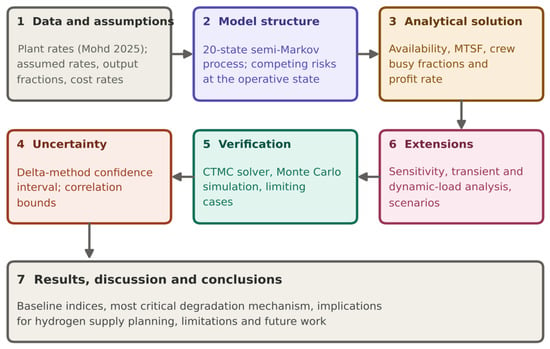
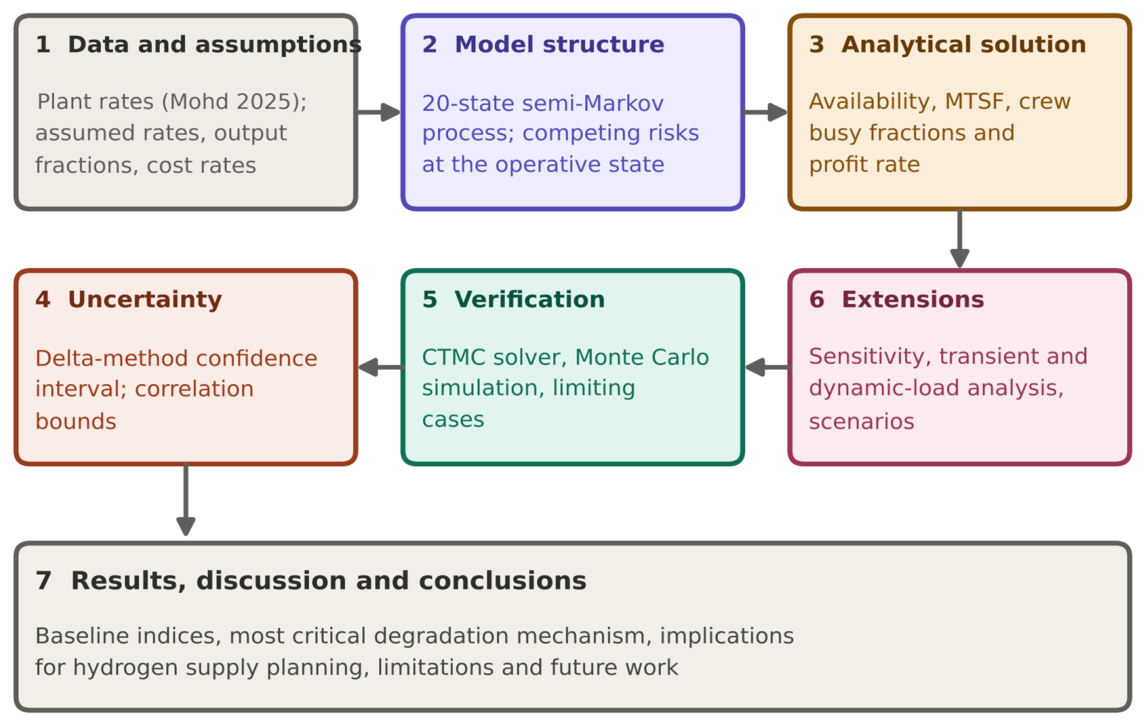
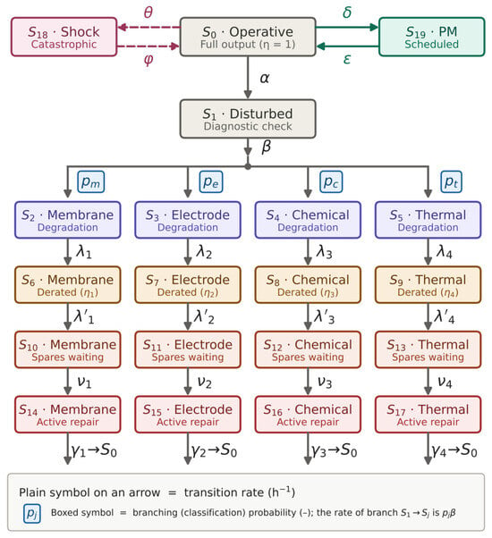
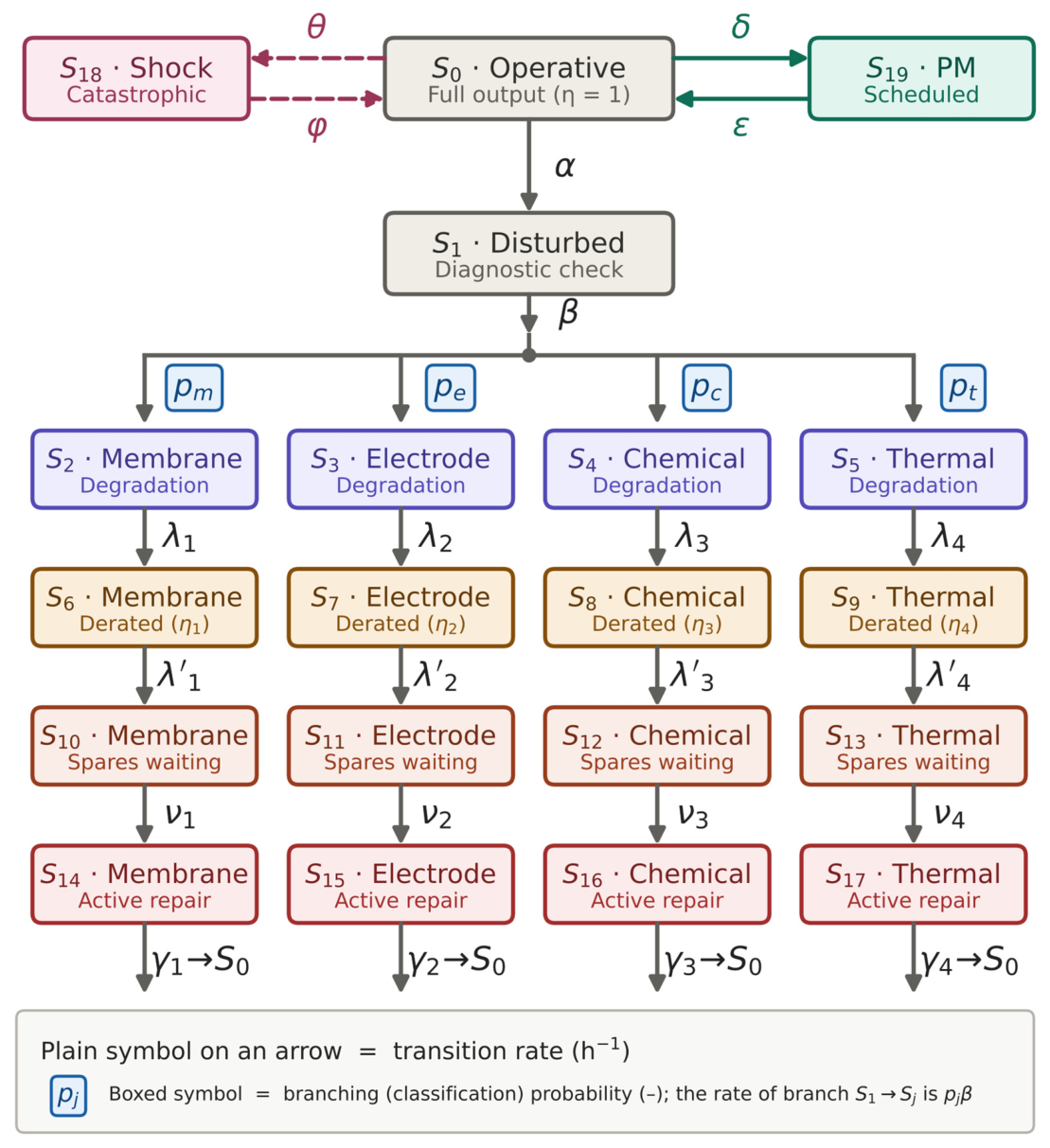
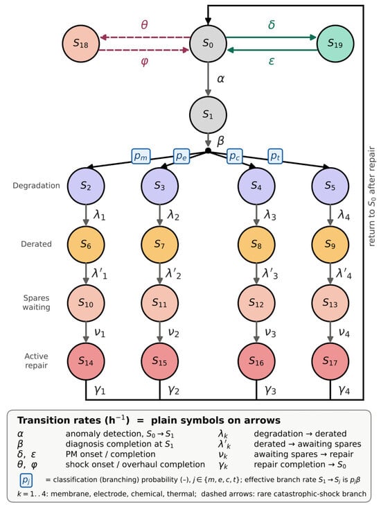
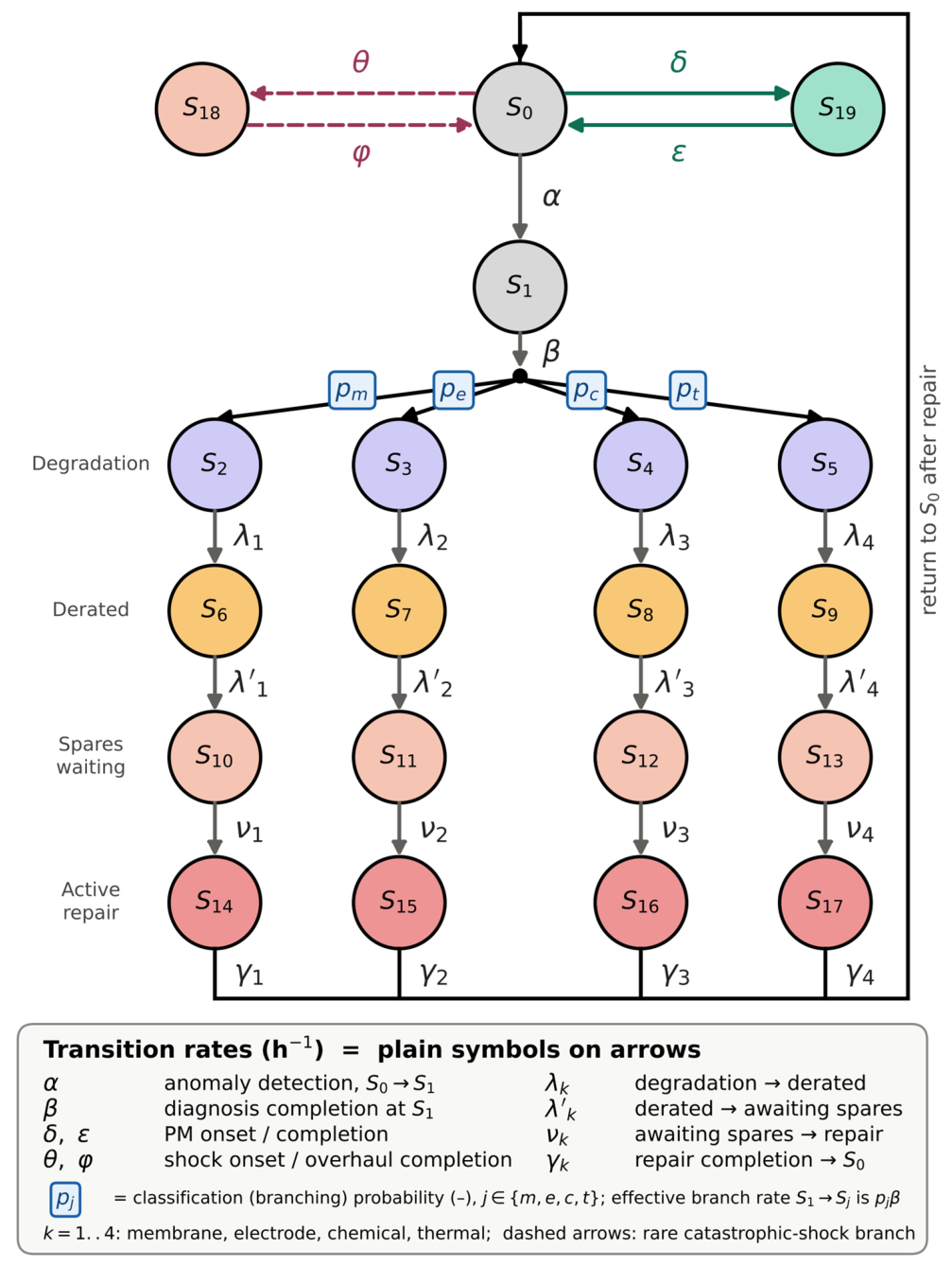
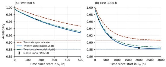
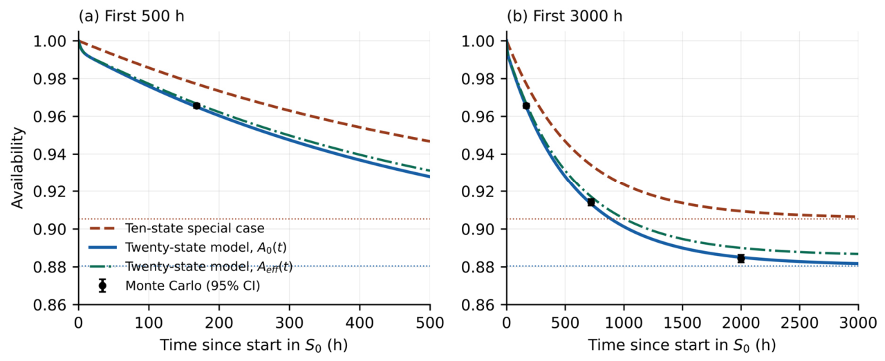
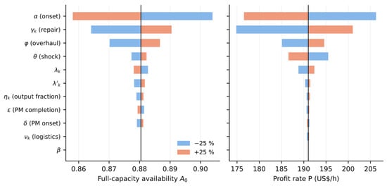
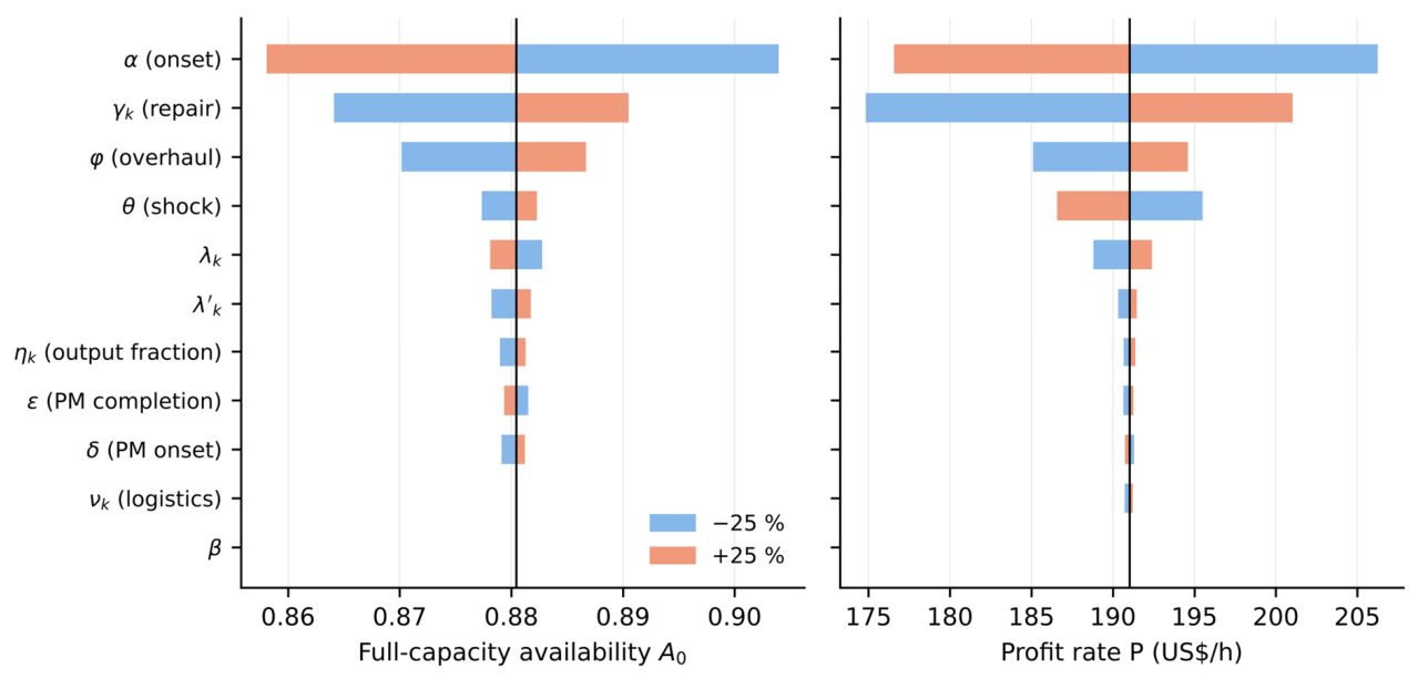
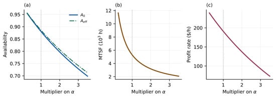
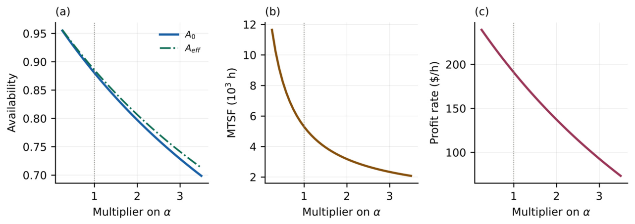
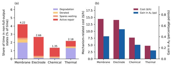
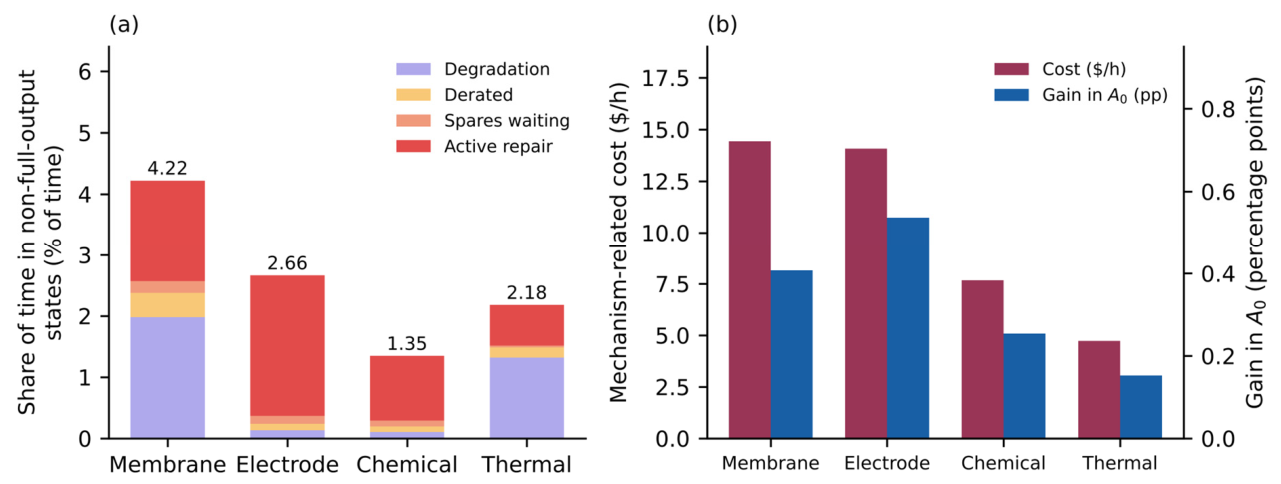
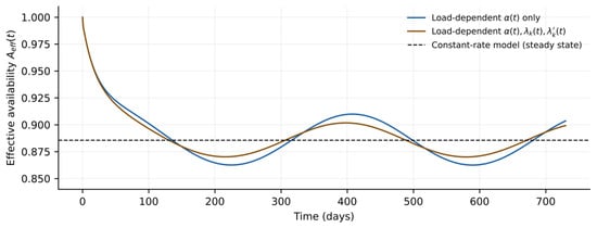
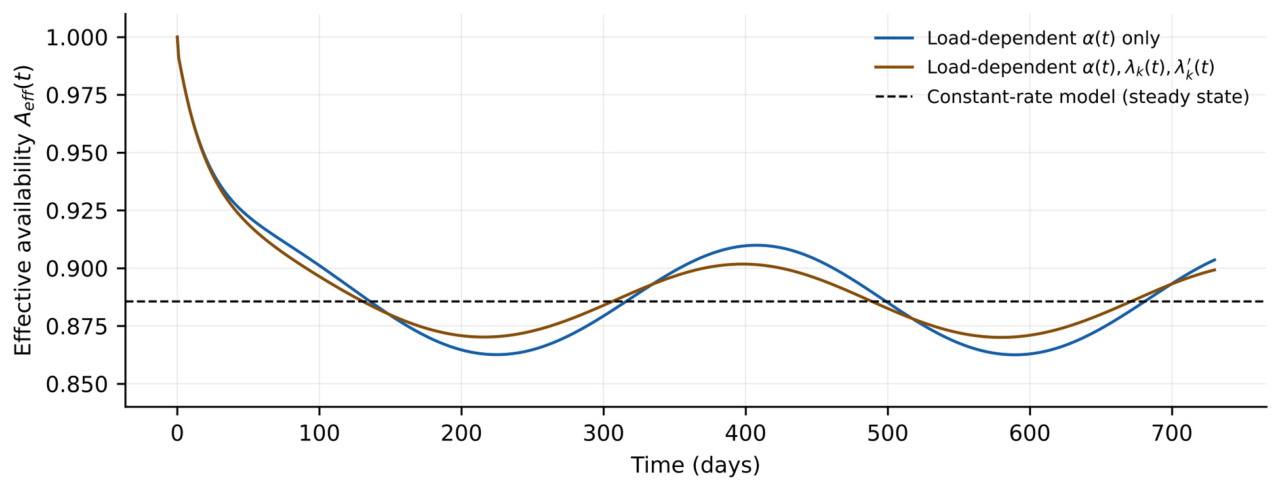

Disclaimer/Publisher’s Note: The statements, opinions and data contained in all publications are solely those of the individual author(s) and contributor(s) and not of MDPI and/or the editor(s). MDPI and/or the editor(s) disclaim responsibility for any injury to people or property resulting from any ideas, methods, instructions or products referred to in the content. |
© 2026 by the authors. Licensee MDPI, Basel, Switzerland. This article is an open access article distributed under the terms and conditions of the Creative Commons Attribution (CC BY) license.