Wind Resource Assessment Using Measured and ERA5 Data for Wind Turbine Performance Evaluation at a Coastal Site in South Korea

Abstract

This study evaluates the wind energy potential and coastal wind turbine suitability at a coastal site in South Korea using two-year measured wind data and ERA5 reanalysis data. Wind characteristics, Weibull parameters, wind power density, and turbine energy performance were analyzed using Windographer. ERA5 showed similar seasonal and directional patterns to the measured data, supporting its use for wind resource comparison and validation over the available measurement period. Among four candidate turbines, the Vestas V112-3.0 MW achieved the highest Net AEP, while the GE 1.7-100 showed the highest NCF. Finally, the CRITIC–TOPSIS method was applied using five technical and energy criteria, identifying the Vestas V112-3.0 MW as the highest-ranked under the selected technical–energy criteria with a closeness coefficient of 0.5547.

1. Introduction

Among renewable energy resources, wind energy is recognized as a sustainable and environmentally friendly source of electricity generation [1]. Accurate assessment of wind energy potential requires a comprehensive analysis of wind characteristics, including wind speed, wind direction, and their temporal variations. Wind speed is highly variable and changes over minutes, hours, days, seasons, and years. Therefore, at least one year of wind measurements is generally recommended to obtain reliable estimates of wind energy potential. However, long-term wind measurements are both costly and time-consuming, making them impractical for many wind energy projects. In such cases, short-term on-site wind measurements are commonly correlated with long-term reference datasets (e.g., ERA5 or MERRA-2) using measure-correlate-predict (MCP) approaches to estimate long-term wind conditions and improve the accuracy of wind resource assessment [2,3]. Because wind characteristics vary with geographical location and seasonal conditions, statistical models such as the Weibull distribution are widely employed to characterize wind regimes, evaluate wind resources, and assess wind turbine performance [1,4]. Once the wind resource at a given site is adequately characterized, the next critical step in offshore wind farm development is the selection of a suitable wind turbine. Although offshore wind energy is increasingly recognized as a promising solution to the growing global demand for renewable energy, its development still involves several technical and engineering challenges. Turbine characteristics can significantly influence project feasibility, operational reliability, and compatibility with site-specific environmental conditions [5]. Turbine selection therefore requires the simultaneous consideration of multiple technical, economic, safety, and environmental criteria, and conventional selection approaches may not adequately capture the interactions and trade-offs among these factors. Consequently, multi-criteria decision-making (MCDM) and other advanced analytical approaches can provide a more systematic framework for evaluating and selecting suitable offshore wind turbine alternatives [6]. In South Korea, there has been an active push to develop offshore wind farms. Compared with onshore wind farms, offshore locations benefit from stronger and more stable wind resources and encounter fewer land-use and compensation constraints, making them attractive for long-term renewable energy development [7]. Case studies in South Korea have shown that the economic feasibility of offshore wind projects is highly dependent on energy production and electricity market prices. To support renewable energy development, the Korean government operates the Renewable Energy Certificate (REC) system, which assigns weighting factors based on technology type, distance from shore, and water depth [8]. Despite the growing body of research on offshore wind energy in South Korea, most existing studies address wind resource assessment and turbine selection as separate problems, and relatively few have combined multi-height, site-specific measurements with reanalysis-based long-term correlation and a systematic multi-criteria turbine selection framework. This gap motivates the integrated approach adopted in the present study.

This study is therefore organized around two main components. First, the wind resource potential of a coastal site in South Korea is evaluated using measured multi-height wind data together with ERA5 reanalysis data extracted from the nearest grid point. Wind characteristics, Weibull parameters, wind power density, and annual energy production (AEP) are analyzed using Windographer software Version 6.0.7, and the agreement between the measured and ERA5 datasets is quantitatively assessed over the common period to examine the representativeness of the reanalysis data at the site. Second, an appropriate coastal wind turbine is selected among several candidate models using an integrated CRITIC–TOPSIS multi-criteria decision-making approach, based on the wind characteristics obtained from the first part. Together, these two components provide a practical framework that combines wind resource assessment with wind turbine selection to support future coastal wind energy development in South Korea. The present study focuses on the technical and energy-yield aspects of turbine selection; economic, safety, environmental, and offshore-specific criteria (e.g., water depth, foundation, corrosion, and certification) are outside its scope.

2. Description of Location and Data

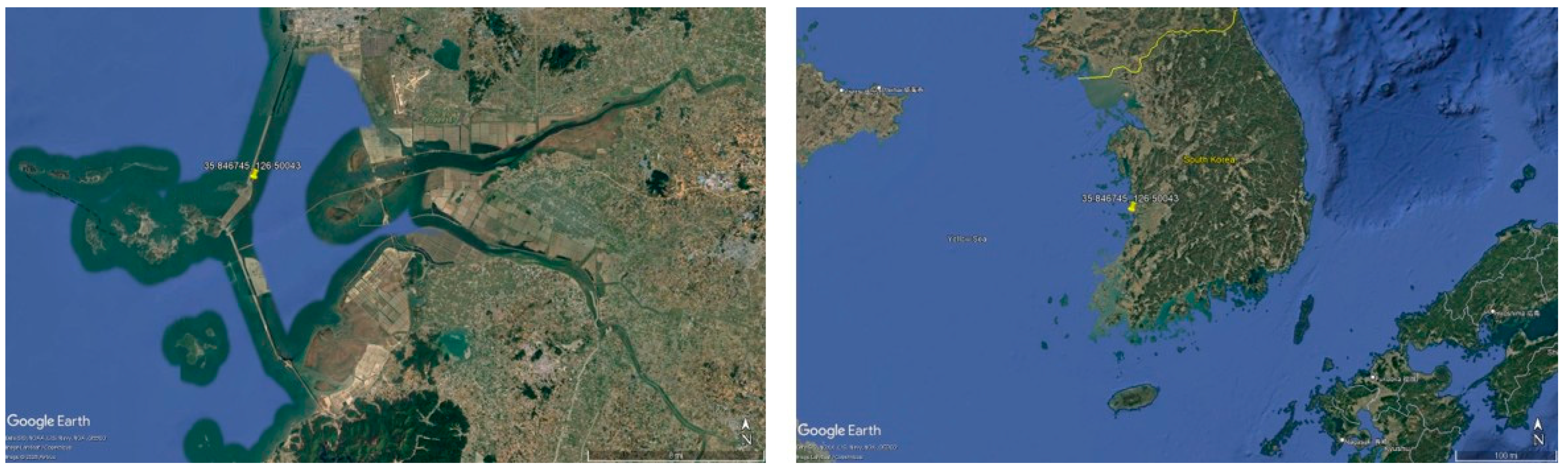
The wind data used in this study were collected from a measurement site located at latitude 35.846745° N and longitude 126.50043° E in South Korea. These locations are shown in Figure 1. An approximately 25-month wind dataset was obtained from a meteorological measurement system installed at the study site, covering the period from 20 June 2017 to 31 July 2019. Wind speed measurements were recorded at multiple heights of 40 m, 60 m, and 80 m above ground level to investigate vertical variations in wind characteristics. The dataset includes the average, maximum, minimum, and standard deviation of wind speed recorded at 10 min intervals. In addition, wind direction and air temperature were continuously monitored throughout the measurement period. Data completeness was assessed using the data recovery rate. For the 80 m wind speed, the overall recovery rate was 99.66% (110,703 valid records out of 111,076 possible 10 min records), and monthly values never fell below 91.6%. Quality control was performed by the authors using Windographer: missing-value records (flagged as 9999) and icing-flagged records were excluded, and only valid data were used in the analysis. The measured and ERA5 time series were referenced to the same time zone (UTC+9, Korea Standard Time), with time stamps indicating the beginning of each time step. The 10 min measurement records were compared with the hourly ERA5 data at a common one-hour time step. ERA5 reanalysis data were obtained using the Windographer Data Downloader. ERA5, developed by the European Centre for Medium-Range Weather Forecasts (ECMWF), is a global atmospheric reanalysis dataset that provides consistent hourly meteorological data by combining observations with numerical weather prediction models, and it is widely used for wind resource assessment and climate studies [9]. The ERA5 grid point nearest to the measurement site (35.750000° N, 126.500000° E; horizontal resolution of 0.25°, approximately 10.7 km south of the site) was selected, and the wind speed at 100 m was used. The full ERA5 record, from 1 January 1979 to 15 June 2026, was used to describe the long-term wind climate at the grid point.

Figure 1. Geographic locations of the Wind Measurement Tower and the study area.

Windographer Software

Windographer is specialized software for processing, analyzing, and visualizing wind resource data. It supports data quality control, statistical analysis, wind rose generation, Weibull distribution fitting, wind shear analysis, and wind turbine energy production assessment. In this study, it was used for quality control and vertical extrapolation of the measured data, for the comparison between measured and ERA5 data, for the characterization of the wind resource, and for the evaluation of the energy production of the selected wind turbines.

3. Methodology

3.1. Wind Analysis Model

Wind is generated primarily by spatial variations in atmospheric pressure resulting from the uneven heating of the Earth’s surface by solar radiation. The resulting movement of air contains kinetic energy, which can be converted into mechanical energy through a wind energy conversion system (WECS). The available power in the wind represents the rate at which kinetic energy passes through a given area and can be expressed as Equation (1) [10]:

$$\mathrm{P}\_\mathrm{w}={\displaystyle \frac{1}{2}}\rho \mathrm{S}\_\mathrm{W}{v}^3$$

(1)

where P_w is the available wind power (W), ρ is the air density (kg/m³), S_W is the rotor swept area (m²), and v is the wind speed (m/s).

For many years, scientists have used the Weibull distribution to represent wind speed distribution in order to calculate wind loads. The wind speed distribution is expressed by a probability density function (also referred to as the wind speed frequency curve), and the two-parameter Weibull function can be calculated as shown in Equation (2) [10]:

$$f\left(v\right)={\displaystyle \frac{k}{A}}\cdot {\left({\displaystyle \frac{v}{A}}\right)}^{k-1}\cdot \mathit{exp}\left[-{\left({\displaystyle \frac{v}{A}}\right)}^k\right]$$

(2)

where f(v) is the probability of observed wind speed v (m/s), k is the dimensionless Weibull shape parameter, and A is the Weibull scale parameter (m/s) (v ≥ 0, k > 0, A > 0). The corresponding cumulative distribution function can be described according to Equation (3) [10]:

$$F\left(v\right)=1-\mathit{exp}\left[-{\left({\displaystyle \frac{v}{A}}\right)}^k\right]$$

(3)

The mean wind speed v_m and standard deviation σ of the distribution are expressed using the Γ function as defined according to Equations (4) and (5) [11]:

$$v\_m=A\cdot \Gamma \left(1+{\displaystyle \frac{1}{k}}\right)$$

(4)

$$\sigma \_v=A\cdot \sqrt{\Gamma \left(1+{\displaystyle \frac{2}{k}}\right)-{\Gamma }^2\left(1+{\displaystyle \frac{1}{k}}\right)}$$

(5)

3.2. Wind Speed Variation with Height

The Hellmann power law equation was applied to extrapolate wind speed between different heights. In this equation, v₁ represents the wind speed measured at height h₁, while v₂ represents the wind speed at height h₂. The wind shear exponent (α) is strongly influenced by surface topography and atmospheric stability conditions near the ground, resulting in characteristic diurnal and annual variations. Higher α values are observed under stable atmospheric conditions, particularly when near-surface temperatures are low, whereas lower values occur under unstable conditions associated with higher temperatures. The exponent is generally higher during nighttime and exhibits a more regular pattern during daytime hours. Based on the above equations, v₂ can be expressed as Equation (6) [12]:

$$v_2=v_1{\left({\displaystyle \frac{h_2}{h_1}}\right)}^{\alpha }$$

(6)

3.3. Wind Turbine Energy Production

The annual energy production (AEP) follows from the turbine power curve P_T(v) (kW) and the wind speed probability density f(v) of Equations (2) and (7) [13]:

$$\mathrm{AEP}=8760{\int }_0^{\mathrm{\infty }}{P}_T\left(v\right)·f\left(v\right)\mathit{dv}$$

(7)

where P_T(v) is the turbine power curve (kW), and f(v) is the Weibull probability density function of Equation (2).

The capacity factor (CF) is calculated using Equation (8) [14]:

$$\mathit{CF}={\displaystyle \frac{\mathit{AEP}}{P_{\mathit{rated}}·8760}}$$

(8)

where CF is the capacity factor (dimensionless), AEP is the annual energy production (kWh/year), P_rated is the rated power of the turbine (kW), and 8760 is the number of hours in a year. Equations (7) and (8) define the gross (theoretical) AEP and capacity factor, i.e., before any losses. In Section 5, the corresponding net quantities (Net Power, Net AEP, and net capacity factor (NCF)) are obtained after applying an overall loss factor, as defined there.

4. Results and Discussion

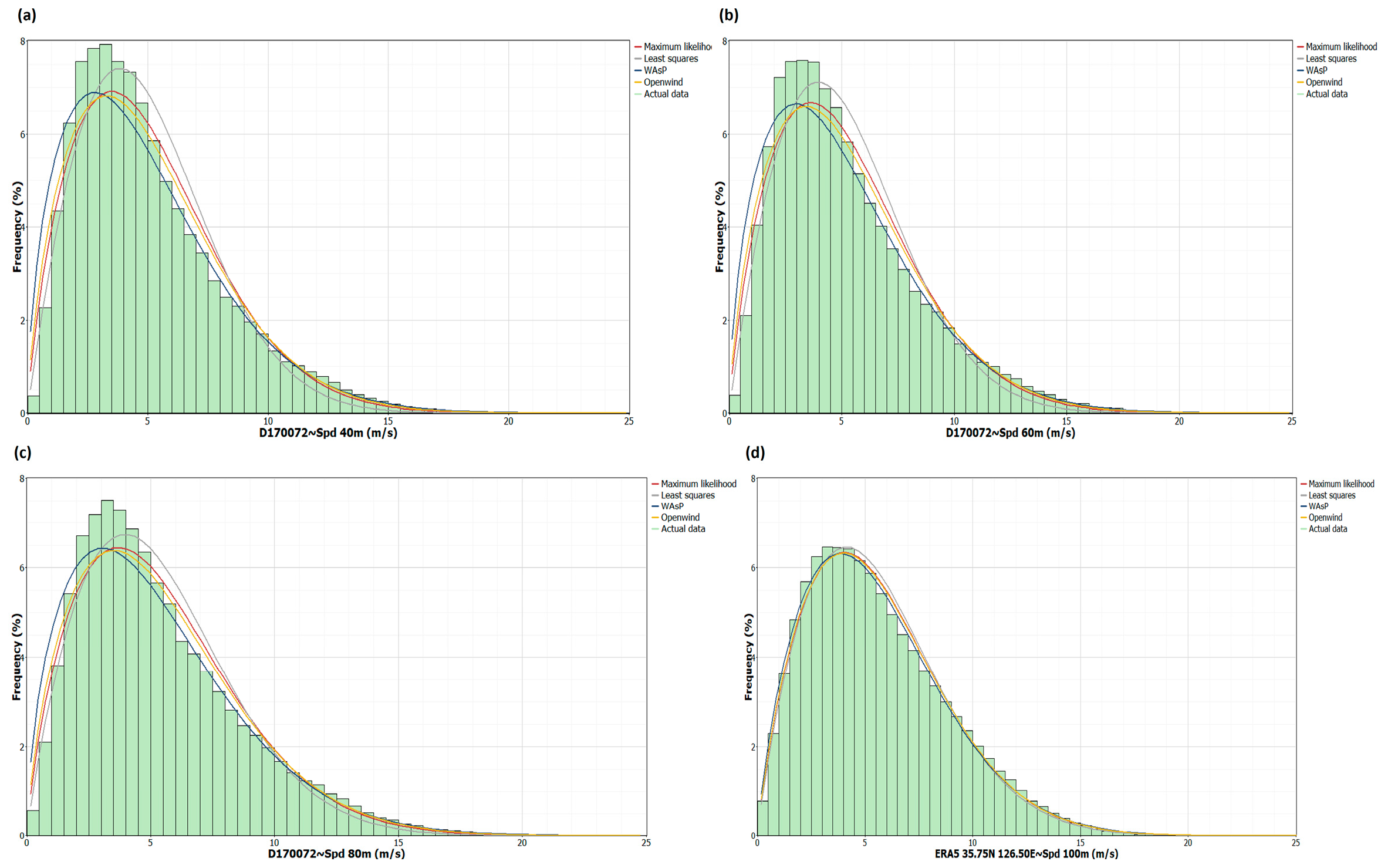
The wind speed frequency histogram represents the percentage of occurrence of wind speeds within different speed intervals. This graphical representation provides a clear description of the wind speed distribution at the study site and allows the most frequently occurring wind speed range to be identified. Such frequency distributions are widely used in wind resource assessment and can also be fitted using statistical models, particularly the Weibull distribution [15]. The wind resource characteristics and the corresponding Weibull parameters obtained using four estimation algorithms are summarized in Table 1 and Table 2 for the measured wind data and the ERA5 reanalysis dataset, respectively. The corresponding wind speed frequency distributions and fitted Weibull curves are presented in Figure 2. The Maximum Likelihood estimates are quoted in the discussion below. As shown in Table 1, the wind resource characteristics improved with increasing measurement height. Since wind speed generally increases with elevation, increasing the hub height can enhance the available wind energy. Given that wind power varies approximately with the cube of wind speed, even a modest increase in wind speed at higher hub heights can lead to a considerable improvement in power generation [16].

Table 1. Wind resource characteristics and Weibull distribution parameters of the measured wind data at 40, 60, and 80 m.

Algorithm	Weibull k	Weibull A (m/s)	Mean (m/s)	Proportion Above 5.069	Power Density (W/m2)	R2	Height (m)
Maximum likelihood	1.740	5.711	5.088	0.444	179.7	0.9701	40
Least squares	1.919	5.634	4.997	0.442	152.4	0.9650
WAsP	1.553	5.457	4.907	0.410	187.2	0.9506
Openwind	1.669	5.674	5.069	0.437	187.2	0.9675
Algorithm	Weibull k	Weibull A (m/s)	Mean (m/s)	Proportion Above 5.252	Power Density (W/m2)	R2	Height (m)
Maximum likelihood	1.742	5.917	5.271	0.444	199.5	0.9713	60
Least squares	1.906	5.842	5.184	0.442	171.3	0.9662
WAsP	1.567	5.674	5.098	0.412	207.2	0.9552
Openwind	1.675	5.880	5.252	0.437	207.2	0.9693
Algorithm	Weibull k	Weibull A (m/s)	Mean (m/s)	Proportion Above 5.421	Power Density (W/m2)	R2	Height (m)
Maximum likelihood	1.727	6.103	5.440	0.443	221.6	0.9750	80
Least squares	1.843	6.044	5.370	0.441	197.5	0.9730
WAsP	1.568	5.867	5.271	0.413	228.9	0.9624
Openwind	1.669	6.068	5.421	0.437	228.9	0.9737

Figure 2. Wind speed frequency distributions and fitted Weibull curves for the measured wind data at 40 (a), 60 (b), and 80 m, (c) and the ERA5 reanalysis dataset at 100 m (d).

Table 2. Wind resource characteristics and Weibull distribution parameters of the ERA5 reanalysis dataset at 100 m.

Algorithm	Weibull k	Weibull A (m/s)	Mean (m/s)	Proportion Above 5.635	Power Density (W/m2)	R2	ERA5 100 m
Maximum likelihood	1.796	6.341	5.640	0.445	235.7	0.9963
Least squares	1.841	6.310	5.605	0.444	225.5	0.9947
WAsP	1.747	6.270	5.585	0.436	236.5	0.9969
Openwind	1.786	6.333	5.635	0.444	236.5	0.9966

Table 2. Wind resource characteristics and Weibull distribution parameters of the ERA5 reanalysis dataset at 100 m.

Algorithm	Weibull k	Weibull A (m/s)	Mean (m/s)	Proportion Above 5.635	Power Density (W/m2)	R2	ERA5 100 m
Maximum likelihood	1.796	6.341	5.640	0.445	235.7	0.9963
Least squares	1.841	6.310	5.605	0.444	225.5	0.9947
WAsP	1.747	6.270	5.585	0.436	236.5	0.9969
Openwind	1.786	6.333	5.635	0.444	236.5	0.9966

The mean wind speed estimated by the Maximum Likelihood method increased from 5.09 m/s at 40 m to 5.44 m/s at 80 m, while the corresponding wind power density increased from 179.7 to 221.6 W/m². Likewise, the Weibull scale parameter increased from 5.71 to 6.10 m/s, indicating stronger wind conditions at higher elevations. The ERA5 reanalysis dataset showed a similar distribution pattern to the measured data, with only a small overall difference in wind resource characteristics, as confirmed by the statistical comparison presented later in this section. As illustrated in Figure 2, the fitted Weibull curves reproduce the overall positively skewed shape of the observed histograms (R² = 0.951–0.975 for the measured data and 0.995–0.997 for ERA5; Table 1 and Table 2), with the highest frequency occurring at moderate wind speeds and a gradual decline toward higher wind speeds. For the measured data, the differences among the fits are largest at low wind speeds and near the mode, and the WAsP fit has the lowest R² at all three heights.

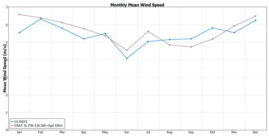
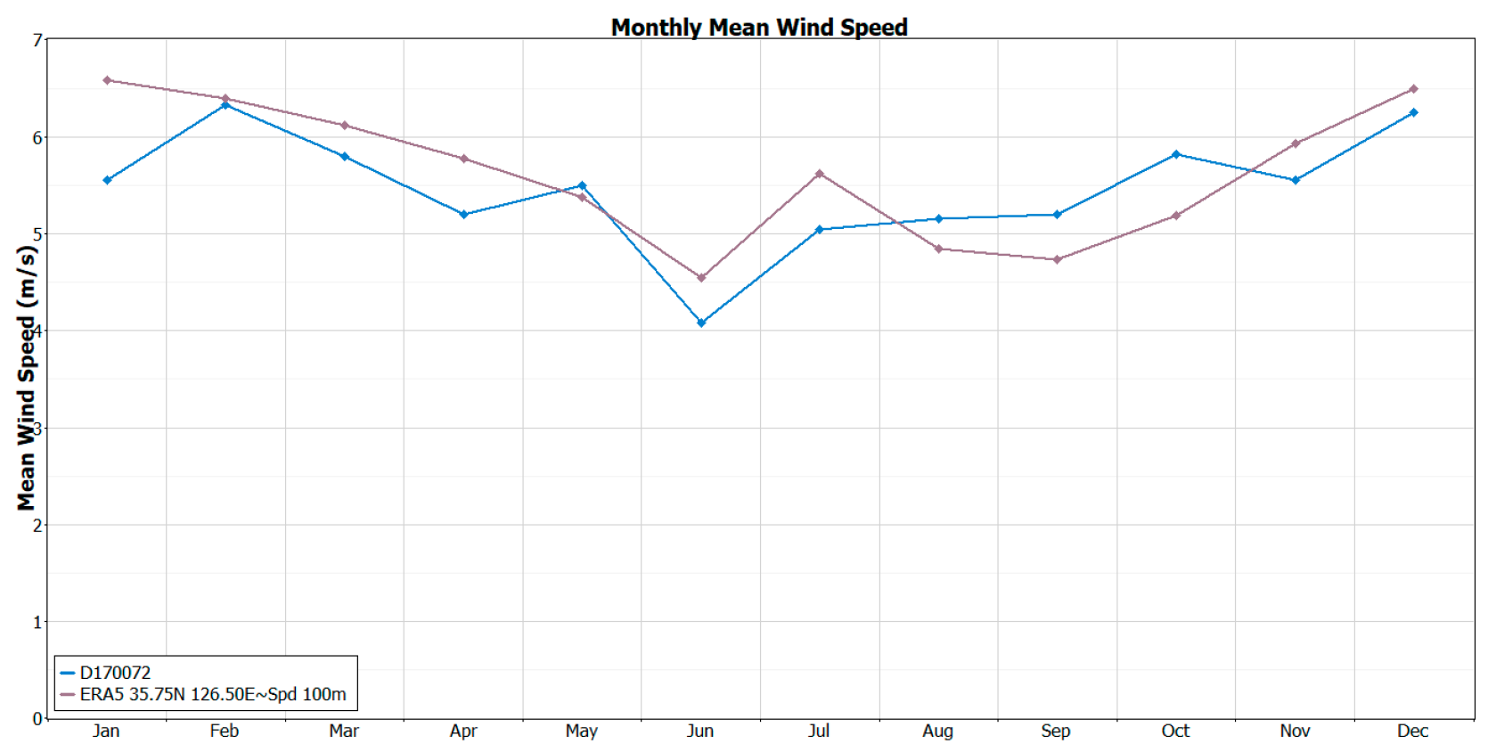
Seasonal variations in wind speed show a consistent pattern across both the measured and ERA5 datasets, as illustrated in Figure 3 and summarized in Table 3. The highest wind speeds were observed during winter, while the lowest occurred in summer. For the measured data, the seasonal mean wind speed increased with height, reaching 6.046 m/s at 80 m in winter and decreasing to 4.760 m/s in summer. A similar seasonal trend was observed in the ERA5 data at 100 m, with mean wind speeds of 6.491, 5.756, 5.006, and 5.286 m/s in winter, spring, summer, and autumn, respectively. Figure 3 and Table 3 are descriptive comparisons of the seasonal and monthly patterns at the native heights of each dataset (measured data at 40, 60, and 80 m and ERA5 data at 100 m), without height correction.

Figure 3. Comparison of monthly mean wind speeds between the measured data at 80 m and the ERA5 reanalysis dataset at 100 m (native heights, no height correction).

Table 3. Seasonal mean wind speed at 40, 60, and 80 m and ERA5 at 100 m above ground.

Height (m)	Winter	Spring	Summer	Autumn
80	6.046	5.500	4.760	5.522
60	5.883	5.253	4.606	5.406
40	5.680	5.015	4.427	5.302
ERA5 100	6.491	5.756	5.006	5.286

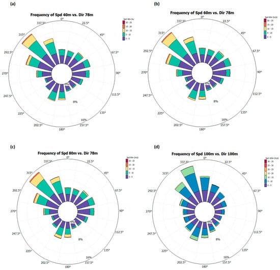
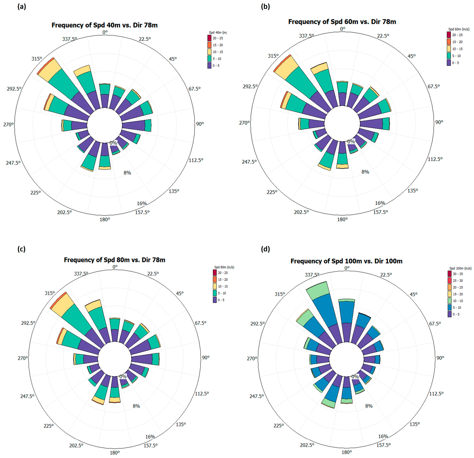
The seasonal and directional agreement between the two datasets indicates that ERA5 reproduces the general seasonal characteristics of the study area over the measurement period. It is therefore used in this study as a long-term reference for comparison, with the hourly-scale uncertainty and the site-representativeness limitations discussed in Section Statistical Validation of ERA5 Against Measured Wind Speed. As shown in Figure 4, a predominant northwesterly wind direction (approximately 300–330°) is observed for both the measured and ERA5 datasets. Similar directional distributions are evident at all measurement heights, indicating that the prevailing wind direction remains relatively stable with increasing height. Although winds occur from most directions, the northwesterly sector contributes the highest frequency and contains a larger proportion of higher wind speeds.

Figure 4. Wind rose diagrams showing the frequency of wind speed by direction sector for the measured data at (a) 40 m, (b) 60 m, and (c) 80 m, and (d) for the ERA5 reanalysis dataset at 100 m. Colors indicate wind speed classes (m/s).

Statistical Validation of ERA5 Against Measured Wind Speed

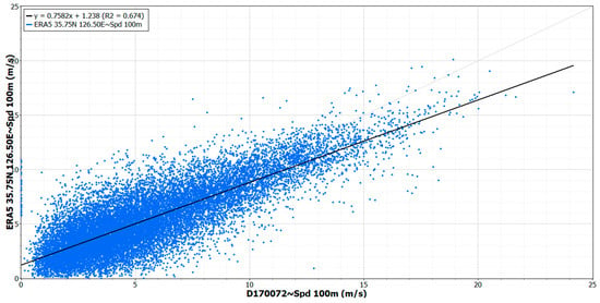
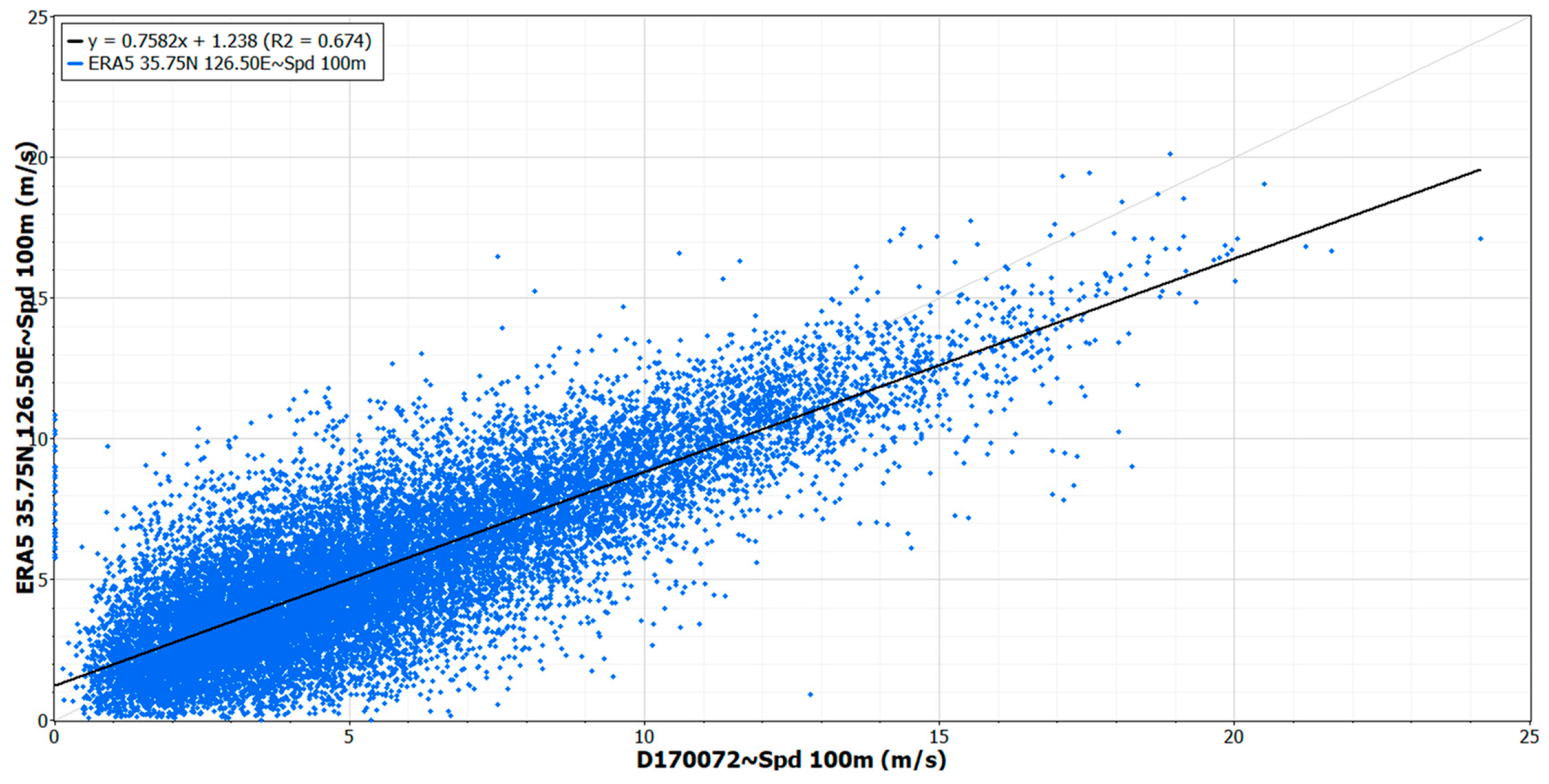
The agreement between ERA5 and reference wind-speed data was quantitatively evaluated using bias, root mean square error (RMSE), and Pearson correlation coefficient (R) [17]. To ensure consistency in measurement height, the measured wind speed at 80 m was extrapolated to 100 m using the Hellmann power law with a monthly power-law exponent lookup table. The resulting time series was then compared with the ERA5 wind speed at 100 m using 18,451 concurrent hourly time steps over the overlapping measurement period. As presented in Table 4, the statistical comparison showed a strong positive correlation (R = 0.821) and a small mean bias (−0.110 m/s). However, the hourly errors are not negligible; the RMSE of 1.941 m/s corresponds to a relative RMSE of 34.8%, and R² = 0.674 (Figure 5) indicates that about one-third of the hourly variance of the measured wind speed is not explained by ERA5. ERA5 therefore reproduces the general variability of the wind speed at the study site, but with a moderate hourly uncertainty.

Table 4. Statistical comparison between measured (extrapolated to 100 m) and ERA5 wind speed at 100 m.

Metric	Value
Number of concurrent hourly pairs (N)	18,451
Mean measured wind speed (m/s)	5.573
Mean ERA5 wind speed (m/s)	5.463
Linear regression (ERA5 vs. measured)	y = 0.7582x + 1.238
Pearson correlation coefficient (R)	0.821
Coefficient of determination (R2)	0.674
Bias, ERA5 − measured (m/s)	−0.110
Root mean square error, RMSE (m/s)	1.941
Mean absolute error, MAE (m/s)	1.487
Relative RMSE (%)	34.8

Figure 5. Comparison of ERA5 and reference wind speeds at 100 m using linear regression.

The error statistics varied with season (Table 5). The agreement was best in autumn and spring (R = 0.846 and 0.842) and weakest in summer (R = 0.752), with relative RMSE = 40.6%, when ERA5 underestimated the measured wind speed on average (bias = −0.239 m/s).

Table 5. Seasonal error statistics of ERA5 against the measured wind speed at 100 m.

Season	N	Bias (m/s)	RMSE (m/s)	MAE (m/s)	R	Relative RMSE (%)
Winter	4320	0.107	2.022	1.563	0.827	32.7
Spring	4416	−0.093	1.957	1.497	0.842	34.2
Summer	5347	−0.239	2.004	1.515	0.752	40.6
Autumn	4368	−0.184	1.755	1.366	0.846	31.3

In addition, ERA5 tended to overestimate low wind speeds and underestimate high wind speeds, as indicated by the regression slope below unity (0.758, Figure 5). Since the energy production varies strongly with wind speed, such errors are particularly relevant for annual energy production estimates. Moreover, these results are based on about 25 months of data at one site and one ERA5 grid point (about 10.7 km from the site), so they validate ERA5 over the measurement period only and do not represent the interannual variability of the site.

5. Technical–Energy Screening of Candidate Wind Turbines

In the development of offshore wind farms, the selection of wind turbines is of great significance. The power quality and economic efficiency of wind farms depend to a large extent on the wind turbines [18]. Currently, there are numerous types of wind turbines on the market, making the selection even more challenging. In addition, the complex marine environment and extreme climate conditions place higher demands on candidate wind turbines than on land [19]. Therefore, greater precision and attention to wind turbine selection are necessary for the long-term development of candidate wind farms, both in terms of power generation capability and revenue potential. The economic influence of wind turbine selection should not be understated, given the prohibitively high cost of offshore wind power development. Previous studies have shown that the power curve is often the most influential factor among selection criteria [20], as it directly determines the overall power production of a wind turbine and, consequently, the return on investment. Since the cost of wind turbines typically constitutes 40–50% of the total investment in offshore wind projects, the initial capital cost also plays a crucial role in turbine selection [20]. Given the large number of parameters involved, the search space for offshore wind turbine selection can be vast [21]. Although wind speed is itself an important selection criterion, achieving high wind farm productivity requires not only installing the most productive turbine but also obtaining precise knowledge of the wind characteristics at a given site. Numerous studies have been conducted to analyze wind energy potential from different perspectives, including site location and turbine type [1,22,23]. The technical specifications of the selected wind turbines, including their original manufacturer-specified hub heights, are presented in Table 6.

Table 6. Main characteristics of the selected wind turbines.

Model	Vestas V100-1.8 MW	GE 1.7-100	Vestas V112-3.0 MW	GAMESA G97-2.0 MW
Rated capacity (kW)	1815	1790	3000	2000
Rotor diameter (m)	100	100	112	97
Hub height (m)	95	96	100	90
Cut-in speed (m/s)	2.50	3.00	2.99	2.00
Rated wind speed (m/s)	12	13	13	14
Cut-out speed (m/s)	20	22	25	25
Swept area (m2)	7854	7854	9852	7389

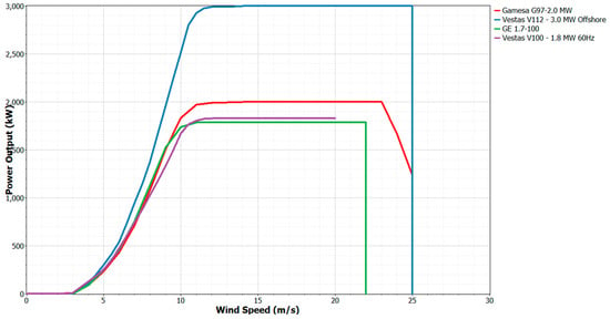
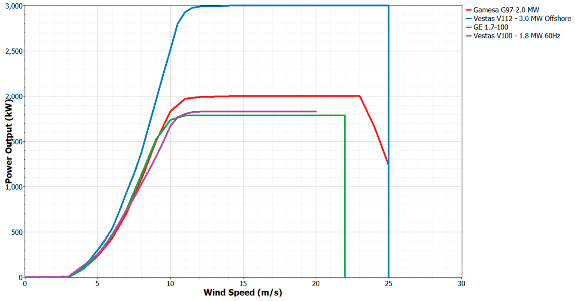
However, to ensure a consistent comparison under the same wind conditions, the performance of all selected turbines was evaluated at a common reference height of 80 m, corresponding to the highest measurement height available at the study site. Therefore, the hub heights listed in Table 6 represent the actual technical specifications of the selected turbines, whereas the 80 m height used in Table 7 represents the reference wind measurement height used for the turbine performance evaluation. This approach allows all selected turbines to be assessed under the same measured wind conditions and minimizes the influence of different hub heights on the comparative evaluation of turbine performance. The effect of hub height on wind speed and energy production has been reported in previous studies [24]. The comparison in Table 7 should therefore be interpreted as a relative, power-curve-based ranking of the candidate turbines under the same wind resource, rather than as a prediction of their absolute energy yield at the actual hub heights (90–100 m), where wind speeds, and hence the net annual energy production (Net AEP) and net capacity factor (NCF), are expected to be higher. Figure 6 illustrates the power curves of the selected turbines. All turbines begin generating power at approximately 2–3 m/s and show a rapid increase in output with increasing wind speed until reaching their rated power. The Vestas V112-3.0 MW achieves the highest rated output (3 MW), while the remaining turbines reach rated outputs between 1.8 and 2.0 MW.

Table 7. Performance comparison of candidate wind turbines evaluated using wind data at the common 80 m reference height. Net Power is the mean loss-adjusted power output; Net AEP = Net Power × 8760 h; NCF (net capacity factor) = Net Power / rated capacity (Table 6); Time at Rated/Zero Power is the percentage of valid time steps at rated or zero output.

Turbine Model	Net Power (kW)	Net AEP (kWh/Year)	NCF (%)	Time at Rated Power (%)	Time at Zero Power (%)
Vestas V100-1.8 MW	418.6	3,667,278	23.07	6.79	18.81
GE 1.7-100	425.4	3,726,166	23.76	5.08	25.88
Vestas V112-3.0 MW	593.5	5,199,358	19.78	2.04	25.69
GAMESA G97-2.0 MW	435.5	3,814,732	21.77	2.04	12.01

Figure 6. Power curves of the four candidate wind turbines as a function of wind speed.

Power curves and AEP calculation: The power curves of the four turbines (Figure 6) were taken from the built-in turbine library of Windographer and are defined at standard air density (1.225 kg/m³). Energy production was calculated in Windographer from the measured 10 min wind speed time series at 80 m (110,703 valid time steps; mean wind speed 5.42 m/s). The option “Adjust for air density” was enabled to account for variations in air density based on the measured meteorological data. The hub heights and rated powers in Table 6 correspond to these library entries. An overall loss factor of 16.005% was applied, combining multiplicatively availability (3%), wake (6%), turbine performance (6%), and electrical (2%) losses; environmental, curtailment, and other losses were set to 0%. These are screening-level assumed values, identical for all turbines. Net Power is the simple mean of the loss-adjusted power output over all valid time steps (Net AEP = Net Power × 8760 h), and the net capacity factor (NCF) is Net Power divided by the rated capacity in Table 6. Time at Zero/Rated Power is the percentage of valid time steps with zero or rated output. The performance results presented in Table 7 show that the Vestas V112-3.0 MW produced the highest Net Power (593.5 kW) and Net AEP (5.20 GWh/year). However, the GE 1.7-100 achieved the highest NCF (23.76%), meaning that its output is the highest relative to its own rated capacity. Since the candidate turbines have different rated capacities and specific powers, NCF should not be read as a measure of absolute energy production: the Vestas V112-3.0 MW, with the highest rated power, produced the highest Net AEP, whereas the GE 1.7-100, with a low specific power, operated closer to its rated capacity.

5.1. Decision Problem and Initial Decision Matrix

The turbine ranking presented in this study is intended as a preliminary screening of candidate turbines rather than a final determination of the most suitable turbine for offshore deployment. Offshore wind turbine selection involves the simultaneous consideration of multiple and often conflicting criteria, making it a multi-criteria decision-making (MCDM) problem. MCDM methods provide a systematic and transparent framework for evaluating such criteria and identifying the most suitable turbine alternative [25]. The multi-attribute decision-making (MADM) method specifically deals with decision problems where the criteria are attributes of a set of discrete alternatives; it aids decision-makers in making an optimal choice by evaluating and weighing these attributes [26,27]. In the context of offshore wind turbine selection, multi-attribute decision-making methods can play a crucial role, since numerous factors need to be considered and a best candidate must be picked [20]. To address this need, the present study developed an integrated CRITIC–TOPSIS framework.The initial decision matrix, containing the five selected criteria for the four candidate turbines, is presented in Table 8.

Table 8. Initial decision matrix for wind turbine selection using TOPSIS.

Turbine Model	Rated Power (kW)	Net AEP (kWh/Year)	Rated Wind Speed (m/s)	Cut-In Speed (m/s)	Rotor Diameter (m)
Vestas V100-1.8 MW	1815	3,667,278	12	2.50	100
GE 1.7-100	1790	3,726,166	13	3.00	100
Vestas V112-3.0 MW	3000	5,199,358	13	2.99	112
GAMESA G97-2.0 MW	2000	3,814,732	14	2.00	97

In this study, five criteria were selected and classified as benefit or cost criteria based on their preference direction. Rated power, net annual energy production (AEP), and rotor diameter were treated as benefit criteria (higher values preferred), while rated wind speed and cut-in wind speed were treated as cost criteria (lower values preferred). An integrated CRITIC–TOPSIS approach [28,29,30] was employed to objectively rank the candidate wind turbines. Some of these criteria are physically related: net AEP depends on the rated power, rotor diameter, power curve, and characteristic wind speeds, so the criteria partly carry overlapping information. This is confirmed by the correlation matrix, with pairwise coefficients of 0.995 (rated power–AEP), 0.930 (rated power–rotor diameter), and 0.958 (AEP–rotor diameter). Such redundancy could inflate the combined influence of these criteria. The CRITIC method partly accounts for this effect because the term (1 − ρ_jk) in Equation (13) reduces the information content of criteria that are strongly correlated with the others [29]. TOPSIS ranks alternatives based on their relative closeness to an ideal solution and distance from the least desirable one, while CRITIC objectively determines criterion weights by considering both variability and inter-criterion correlation. Integrating CRITIC with TOPSIS thus provides a systematic framework in which objective weights are incorporated directly into the ranking process [29,30].

5.2. Objective Criteria Weights Using CRITIC

Normalize the decision matrix using the TOPSIS vector normalization formula as shown in Equation (9) [28,29]:

$${\mathit{r}}_{\mathit{ij}}={\displaystyle \frac{{\mathit{x}}_{\mathit{ij}}}{\sqrt{{\displaystyle {\sum }_{\mathit{i}=1}^{\mathit{m}}}{{\mathit{x}}_{\mathit{ij}}}^2}}}$$

(9)

Using the normalized matrix r_ij of Equation (9), the standard deviation of each criterion j, which measures its contrast intensity, was calculated as

$${\mathit{\sigma }}_{\mathit{j}}=\sqrt{{\displaystyle \frac{{\displaystyle {\sum }_{\mathit{i}=1}^{\mathit{m}}}{({\mathit{r}}_{\mathit{ij}}-{\overline{\mathit{r}}}_{\mathit{j}})}^2}{\mathit{m}-1}}}$$

(10)

where the mean of criterion j is

$${\overline{\mathit{r}}}_{\mathit{j}}={\displaystyle \frac{1}{\mathit{m}}}{\displaystyle \sum _{\mathit{i}=1}^{\mathit{m}}}{\mathit{r}}_{\mathit{ij}}$$

(11)

The conflict between criteria was quantified through the Pearson correlation coefficient between each pair of criteria j and k:

$${\mathit{\rho }}_{\mathit{jk}}={\displaystyle \frac{{\displaystyle {\sum }_{\mathit{i}=1}^{\mathit{m}}}({\mathit{r}}_{\mathit{ij}}-{\overline{\mathit{r}}}_{\mathit{j}})({\mathit{r}}_{\mathit{ik}}-{\overline{\mathit{r}}}_{\mathit{k}})}{\sqrt{{\displaystyle {\sum }_{\mathit{i}=1}^{\mathit{m}}}{({\mathit{r}}_{\mathit{ij}}-{\overline{\mathit{r}}}_{\mathit{j}})}^2·{\displaystyle {\sum }_{\mathit{i}=1}^{\mathit{m}}}{({\mathit{r}}_{\mathit{ik}}-{\overline{\mathit{r}}}_{\mathit{k}})}^2}}}$$

(12)

The information content of criterion j combines its variability and its conflict with the other criteria:

$${\mathit{C}}_{\mathit{j}}={\mathit{\sigma }}_{\mathit{j}}·{\displaystyle \sum _{\mathit{k}=1}^{\mathit{n}}}(1-{\mathit{\rho }}_{\mathit{jk}})$$

(13)

where m = 4 is the number of alternatives, and n = 5 is the number of criteria. A criterion that is strongly correlated with the others obtains a small Σ(1 − ρ_jk) and hence a lower information content. The objective weights were then obtained by normalization [29]:

$${\mathit{w}}_{\mathit{j}}={\displaystyle \frac{{\mathit{C}}_{\mathit{j}}}{{\displaystyle {\sum }_{\mathit{k}=1}^{\mathit{n}}}{\mathit{C}}_{\mathit{k}}}}$$

(14)

A criterion therefore receives a high weight when it discriminates strongly among the alternatives and is weakly or negatively correlated with the other criteria [29]. In this study, the CRITIC weights were computed from the vector-normalized matrix of Equation (9) without direction adjustment of the cost criteria, and the same normalized matrix was then used in TOPSIS. The criteria types and the resulting CRITIC weights are listed in Table 9.

Table 9. Criteria and objective CRITIC weights.

Criterion	Type	CRITIC Weight
Rated Power	Benefit (+)	0.2578
Net AEP	Benefit (+)	0.1677
Rated wind speed	Cost (−)	0.1750
Cut-in wind speed	Cost (−)	0.3321
Rotor Diameter (m)	Benefit (+)	0.0674
Total		1.0000

5.3. Ranking of the Alternatives Using TOPSIS

The weighted normalized matrix was computed by multiplying the normalized matrix of Equation (9) by the CRITIC weights of Table 9 [28,31]:

v_ij= w_j· r_ij

(15)

The positive and negative ideal solutions were defined as the best and worst values of each criterion, taking the benefit or cost nature of each criterion into account:

$${\mathit{v}}_{\mathit{j}}^{+}={\mathit{max}}_{\mathit{i}}{\mathit{v}}_{\mathit{ij}},{\mathit{v}}_{\mathit{j}}^{-}={\mathit{min}}_{\mathit{i}},\left(\mathbf{benefit}\right)$$

$${\mathit{v}}_{\mathit{j}}^{+}={\mathit{min}}_{\mathit{i}}{\mathit{v}}_{\mathit{ij}},{\mathit{v}}_{\mathit{j}}^{-}={\mathit{max}}_{\mathit{i}}{\mathit{v}}_{\mathit{ij}},\left(\mathbf{cost}\right)$$

(16)

The separation measure is calculated by determining the n-dimensional Euclidean distance. It is determined by

$${\mathit{S}}_{\mathit{i}}^{+}=\sqrt{{\displaystyle \sum _{\mathit{j}=1}^{\mathit{n}}}{({\mathit{v}}_{\mathit{ij}}-{\mathit{v}}_{\mathit{j}}^{+})}^2}$$

(17)

$${\mathit{S}}_{\mathit{i}}^{-}=\sqrt{{\displaystyle \sum _{\mathit{j}=1}^{\mathit{n}}}{({\mathit{v}}_{\mathit{ij}}-{\mathit{v}}_{\mathit{j}}^{-})}^2}$$

(18)

and the closeness coefficient was

$${\mathit{C}}_{\mathit{i}}={\displaystyle \frac{{\mathit{S}}_{\mathit{i}}^{-}}{({\mathit{S}}_{\mathit{i}}^{+}+{\mathit{S}}_{\mathit{i}}^{-})}}$$

(19)

Alternatives were ranked in descending order of Ci; a higher value indicates a solution closer to the ideal and farther from the anti-ideal solution, and the final ranking is reported in Table 10.

Table 10. Final CRITIC–TOPSIS ranking.

Rank	Turbine Model	Si+	Si−	TOPSIS Score ci
1	Vestas V112-3.0 MW	0.0623	0.0776	0.5547
2	GAMESA G97-2.0 MW	0.0663	0.0638	0.4903
3	Vestas V100-1.8 MW	0.0821	0.0341	0.2934
4	GE 1.7-100	0.0992	0.0069	0.0650

The CRITIC–TOPSIS analysis ranked the Vestas V112-3.0 MW first (C_i = 0.5547), followed by the GAMESA G97-2.0 MW (0.4903), the Vestas V100-1.8 MW (0.2934), and the GE 1.7-100 (0.0650). The CRITIC method assigned the highest weight to cut-in wind speed (0.3321), followed by rated power (0.2578).

Consequently, the superiority of the Vestas V112-3.0 MW is mainly attributable to its combination of the highest rated power (3000 kW) and the highest net AEP (5,199,358 kWh/year) among the candidate turbines. Its cut-in wind speed (2.99 m/s) is not among the lowest, being higher than those of the GAMESA G97-2.0 MW (2.00 m/s) and the Vestas V100-1.8 MW (2.50 m/s) and nearly equal to that of the GE 1.7-100 (3.00 m/s). Therefore, the high weight assigned to cut-in wind speed (0.3321) was reduced but did not eliminate this advantage, and the V112-3.0 MW retained the first rank. This result is consistent with the raw performance comparison in Table 7, in which the V112-3.0 MW also achieved the highest net AEP among the candidate turbines.

5.4. Sensitivity Analysis of the Criteria Weights

A sensitivity analysis based on ±10% criterion-weight variation combined with TOPSIS was performed [32]. The data of Table 8 were kept fixed, and only the CRITIC weights of Table 9 were changed. For each criterion j, the weight was decreased and then increased by 10%, while the other weights were kept at their original values:

$$w_j^{\prime }=w_j(1\pm \delta ),\delta =0.10$$

(20)

For example, for rated power (w₁ = 0.2578), the perturbed weights are 0.2578 × 0.90 = 0.23202 and 0.2578 × 1.10 = 0.28358. Because the weights must sum to one, the weight vector of each scenario was renormalized:

$$w_j^{*}={\displaystyle \frac{w_j^{\prime }}{{\displaystyle {\sum }_{k=1}^n}{w}_k^{\prime }}}$$

(21)

TOPSIS was then recomputed from the weighted matrix onward (Equations (15)–(19)) using the renormalized weights w^∗_j, which yielded ten scenarios. The closeness coefficients and the resulting rankings are reported in Table 11. In all ten scenarios, the ranking of the four turbines remained unchanged (V112-3.0 MW > G97-2.0 MW > V100-1.8 MW > GE 1.7-100), and the Vestas V112-3.0 MW remained first. The ranking is therefore stable under moderate variations in the criteria weights. However, the margin between the first two alternatives was small in the scenarios with a 10% decrease in the rated power weight (0.0239) and a 10% increase in the cut-in wind speed weight (0.0179).

Table 11. TOPSIS scores (C_i) under ±10% variation in each CRITIC weight.

Criterion Varied	Change	V112-3.0 MW	G97-2.0 MW	V100-1.8 MW	GE 1.7-100	Margin 1st–2nd	Ranking
Rated power	−10%	0.5334	0.5095	0.3086	0.0681	0.0239	V112 > G97 > V100 > GE
Rated power	+10%	0.5744	0.4726	0.2793	0.0620	0.1018	V112 > G97 > V100 > GE
Net AEP	−10%	0.5509	0.4947	0.2963	0.0653	0.0562	V112 > G97 > V100 > GE
Net AEP	+10%	0.5587	0.4859	0.2904	0.0646	0.0728	V112 > G97 > V100 > GE
Rated wind speed	−10%	0.5548	0.4914	0.2903	0.0592	0.0634	V112 > G97 > V100 > GE
Rated wind speed	+10%	0.5546	0.4893	0.2968	0.0707	0.0653	V112 > G97 > V100 > GE
Cut-in wind speed	−10%	0.5802	0.4653	0.2785	0.0674	0.1149	V112 > G97 > V100 > GE
Cut-in wind speed	+10%	0.5313	0.5134	0.3074	0.0626	0.0179	V112 > G97 > V100 > GE
Rotor diameter	−10%	0.5546	0.4906	0.2934	0.0649	0.0640	V112 > G97 > V100 > GE
Rotor diameter	+10%	0.5548	0.4903	0.2934	0.0651	0.0645	V112 > G97 > V100 > GE

6. Conclusions

Limitations of transferring coastal tower measurements to offshore applications. The measurements were obtained from a coastal meteorological tower and may not fully represent offshore conditions. Surface roughness over land and the coastal fringe is generally higher and more heterogeneous than over open water, which affects the vertical wind profile; the shear exponents derived here (Hellmann law, Section 3.2) may therefore differ from offshore values, and extrapolation to 100 m carries additional uncertainty. Atmospheric stability also differs offshore, where sea–air temperature differences and the associated stable/unstable conditions modify shear, turbulence, and wind-speed variability. Furthermore, exposure and fetch depend on wind direction, and sea breeze and land–sea thermal contrasts influence the coastal site in ways that are not captured by a single tower or by a single ERA5 grid point located about 10.7 km from the site. Consequently, the resource estimates and the turbine ranking should be interpreted as indicative of this coastal site and as a methodological demonstration. A full offshore suitability assessment would require site-specific offshore data (e.g., floating LiDAR or offshore met-mast measurements), wave and metocean conditions, water depth, foundation and grid-connection considerations, and economic indicators such as LCOE.

This study assessed the wind resource and coastal wind turbine suitability at a coastal site in South Korea using two years of measured wind data, ERA5 reanalysis, and the CRITIC–TOPSIS method. The results showed that wind speed and power density increased with height, reaching 5.44 m/s and 221.6 W/m² at 80 m. ERA5 reproduced similar seasonal and directional patterns, indicating its consistency with the measured wind data over the available measurement period. Among the evaluated turbines, the Vestas V112-3.0 MW achieved the highest Net AEP, while the GE 1.7-100 provided the highest NCF. However, considering multiple technical and energy criteria simultaneously, the CRITIC–TOPSIS method was applied as a technical–energy screening using five criteria, ranking the Vestas V112-3.0 MW first (closeness coefficient 0.5547) under the selected criteria. These findings demonstrate that combining wind resource assessment, turbine performance analysis, and multi-criteria decision-making provides a practical framework for selecting suitable wind turbines for coastal wind development. It should be noted that the present multi-criteria evaluation was based solely on technical and energy-related criteria; economic factors such as capital and operational costs were not included due to data limitations. Incorporating cost-based indicators such as the levelized cost of energy (LCOE) in future studies would enable a more comprehensive techno-economic evaluation and support a more robust turbine selection decision.

References

- Mohamadi, H.; Saeedi, A.; Firoozi, Z.; Sepasi Zangabadi, S.; Veisi, S. Assessment of wind energy potential and economic evaluation of four wind turbine models for the east of Iran. Heliyon 2021, 7, e07234. [Google Scholar] [CrossRef] [Scilit]
- Risdianto, D.; Hesty, N.W.; Zaky, T.; Wijayanto, R.P.; Mayasari, A.P.; Witjakso, A. Small-scale wind turbine selection based on wind energy potential analysis using Windographer. J. Nas. Tek. Elektro Teknol. Inf. 2024, 13, 290–296. [Google Scholar] [CrossRef] [Scilit]
- Carta, J.A.; Velázquez, S.; Cabrera, P. A review of measure-correlate-predict (MCP) methods used to estimate long-term wind characteristics at a target site. Renew. Sustain. Energy Rev. 2013, 27, 362–400. [Google Scholar] [CrossRef] [Scilit]
- Allouhi, A.; Zamzoum, O.; Islam, M.R.; Saidur, R.; Kousksou, T.; Jamil, A.; Derouich, A. Evaluation of wind energy potential in Morocco’s coastal regions. Renew. Sustain. Energy Rev. 2017, 72, 311–324. [Google Scholar] [CrossRef] [Scilit]
- Spiru, P.; Simona, P.L. Wind energy resource assessment and wind turbine selection analysis for sustainable energy production. Sci. Rep. 2024, 14, 10708. [Google Scholar] [CrossRef] [Scilit]
- Xue, J.; Yang, H.; Song, Y.; Zhang, C.; Hu, H. A fuzzy decision-making network model for offshore wind turbine selection based on simulated annealing algorithm. Ocean Eng. 2025, 315, 119816. [Google Scholar] [CrossRef] [Scilit]
- Lee, J.; Xydis, G. Floating offshore wind projects development in South Korea without government subsidies. Clean Technol. Environ. Policy 2024, 26, 1587–1602. [Google Scholar] [CrossRef] [Scilit]
- Ministry of Trade, Industry and Energy (MOTIE). Guidelines on the Management and Operation of the Renewable Portfolio Standard and Mandatory Fuel-Mix System. 2025. Available online: https://www.law.go.kr/LSW/admRulInfoP.do?admRulSeq=2100000259456 (accessed on 18 September 2026).
- Hersbach, H.; Bell, B.; Berrisford, P.; Hirahara, S.; Horányi, A.; Muñoz-Sabater, J.; Nicolas, J.; Peubey, C.; Radu, R.; Schepers, D.; et al. The ERA5 global reanalysis. Q. J. R. Meteorol. Soc. 2020, 146, 1999–2049. [Google Scholar] [CrossRef] [Scilit]
- Bassyouni, M.; Gutub, S.A.; Javaid, U.; Awais, M.; Rehman, S.; Abdel-Hamid, S.M.-S.; Abdel-Aziz, M.H.; Abouel-Kasem, A.; Shafeek, H. Assessment and analysis of wind power resource using Weibull parameters. Energy Explor. Exploit. 2015, 33, 105–122. [Google Scholar] [CrossRef] [Scilit]
- Mohammed, D.; Abdelaziz, A.S.M.; Mohammed, E.; Elmostapha, E. Analysis of wind speed data and wind energy potential using Weibull distribution in Zagora, Morocco. Int. J. Renew. Energy Dev. 2019, 8, 267–273. [Google Scholar] [CrossRef] [Scilit]
- Gualtieri, G. Atmospheric stability varying wind shear coefficients to improve wind resource extrapolation: A temporal analysis. Renew. Energy 2016, 87, 376–390. [Google Scholar] [CrossRef] [Scilit]
- Amlashi, H.; Baniotopoulos, C. A probabilistic approach for the levelized cost of energy of floating offshore wind farms. Discov. Energy 2024, 4, 15. [Google Scholar] [CrossRef] [Scilit]
- Torres-Madroñero, J.L.; Alvarez-Montoya, J.; Restrepo-Montoya, D.; Tamayo-Avendaño, J.M.; Nieto-Londoño, C.; Sierra-Pérez, J. Technological and operational aspects that limit small wind turbines performance. Energies 2020, 13, 6123. [Google Scholar] [CrossRef] [Scilit]
- Seguro, J.V.; Lambert, T.W. Modern estimation of the parameters of the Weibull wind speed distribution for wind energy analysis. J. Wind Eng. Ind. Aerodyn. 2000, 85, 75–84. [Google Scholar] [CrossRef] [Scilit]
- Petrović, A.; Đurišić, Ž. Genetic algorithm based optimized model for the selection of wind turbine for any site-specific wind conditions. Energy 2021, 236, 121476. [Google Scholar] [CrossRef] [Scilit]
- Chen, T.-C.; Collet, F.; Di Luca, A. Evaluation of ERA5 precipitation and 10-m wind speed associated with extratropical cyclones using station data over North America. Int. J. Climatol. 2024, 44, 729–747. [Google Scholar] [CrossRef] [Scilit]
- Maienza, C.; Avossa, A.M.; Picozzi, V.; Ricciardelli, F. Feasibility analysis for floating offshore wind energy. Int. J. Life Cycle Assess. 2022, 27, 796–812. [Google Scholar] [CrossRef] [Scilit]
- Ma, H.; Ge, M.; Wu, G.; Du, B.; Liu, Y. Formulas of the optimized yaw angles for cooperative control of wind farms with aligned turbines to maximize the power production. Appl. Energy 2021, 303, 117691. [Google Scholar] [CrossRef] [Scilit]
- Li, M.; Jiang, X.; Carroll, J.; Negenborn, R.R. A multi-objective maintenance strategy optimization framework for offshore wind farms considering uncertainty. Appl. Energy 2022, 321, 119284. [Google Scholar] [CrossRef] [Scilit]
- Yu, Y.; Wu, S.; Yu, J.; Xu, Y.; Song, L.; Xu, W. A hybrid multi-criteria decision-making framework for offshore wind turbine selection: A case study in China. Appl. Energy 2022, 328, 120173. [Google Scholar] [CrossRef] [Scilit]
- Sanchez Gomez, M.; Lundquist, J.K. The effect of wind direction shear on turbine performance in a wind farm in central Iowa. Wind Energy Sci. 2020, 5, 125–139. [Google Scholar] [CrossRef] [Scilit]
- Quan, P.; Leephakpreeda, T. Assessment of wind energy potential for selecting wind turbines: An application to Thailand. Sustain. Energy Technol. Assess. 2015, 11, 17–26. [Google Scholar] [CrossRef] [Scilit]
- Vasel-Be-Hagh, A.; Archer, C.L. Wind Farm Hub Height Optimization. Appl. Energy 2017, 195, 905–921. [Google Scholar] [CrossRef] [Scilit]
- Xu, L.; Wang, J.; Ou, Y.; Fu, Y.; Bian, X. A novel decision-making system for selecting offshore wind turbines with PCA and D numbers. Energy 2022, 258, 124818. [Google Scholar] [CrossRef] [Scilit]
- Malefaki, S.; Markatos, D.; Filippatos, A.; Pantelakis, S. A comparative analysis of multi-criteria decision-making methods and normalization techniques in holistic sustainability assessment for engineering applications. Aerospace 2025, 12, 100. [Google Scholar] [CrossRef] [Scilit]
- Alinezhad, A.; Khalili, J. ANP method. In New Methods and Applications in Multiple Attribute Decision Making (MADM); Springer International Publishing: Cham, Switzerland, 2019; pp. 115–125. [Google Scholar] [CrossRef] [Scilit]
- Hwang, C.-L.; Yoon, K. Multiple Attribute Decision Making: Methods and Applications—A State-of-the-Art Survey; Lecture Notes in Economics and Mathematical Systems; Springer: Berlin/Heidelberg, Germany, 1981; Volume 186. [Google Scholar] [CrossRef] [Scilit]
- Diakoulaki, D.; Mavrotas, G.; Papayannakis, L. Determining objective weights in multiple criteria problems: The CRITIC method. Comput. Oper. Res. 1995, 22, 763–770. [Google Scholar] [CrossRef] [Scilit]
- Abdel-Basset, M.; Mohamed, R. A novel plithogenic TOPSIS-CRITIC model for sustainable supply chain risk management. J. Clean. Prod. 2020, 247, 119586. [Google Scholar] [CrossRef] [Scilit]
- Behzadian, M.; Otaghsara, S.K.; Yazdani, M.; Ignatius, J. A state-of-the-art survey of TOPSIS applications. Expert Syst. Appl. 2012, 39, 13051–13069. [Google Scholar] [CrossRef] [Scilit]
- Triantaphyllou, E.; Sánchez, A. A sensitivity analysis approach for some deterministic multi-criteria decision-making methods. Decis. Sci. 1997, 28, 151–194. [Google Scholar] [CrossRef] [Scilit]
Disclaimer/Publisher’s Note: The statements, opinions and data contained in all publications are solely those of the individual author(s) and contributor(s) and not of MDPI and/or the editor(s). MDPI and/or the editor(s) disclaim responsibility for any injury to people or property resulting from any ideas, methods, instructions or products referred to in the content. |
© 2026 by the authors. Licensee MDPI, Basel, Switzerland. This article is an open access article distributed under the terms and conditions of the Creative Commons Attribution (CC BY) license.