Aggregate Regulation Regions with Joint Response Calibration and Network Constraints

Abstract

Network-feasible regulation headroom does not ensure that aggregated resources can deliver a dispatch instruction within its activation window. This study combines joint response calibration with robust linear network constraints to construct an aggregate regulation region. A maximum standardized shortfall score provides simultaneous lower response bounds from independent calibration episodes. These bounds enter a robust command-space model, and directional linear programs generate an inner approximation with guaranteed active increment and capacitive reactive support. All results are obtained on the public 33-bus feeder with an explicitly specified synthetic response generator (400 training, 800 calibration and 2000 test episodes per scenario) and are not operational performance figures. In this benchmark, boundary-command delivery failure at 95% nominal coverage ranges from 1.95% to 4.25%; the compound scenario reduces region area by 19.15%, and fixed 0.8 derating yields 11.85% delivery failure there. Sensitivity sweeps over response dispersion, correlation and activation time keep joint-calibrated failure below 5%, whereas fixed derating reaches 39%. Full-boundary AC checks on 2000 episodes show no violation. Under an abrupt response shift, frozen calibration fails in 73% of episodes; an alarm-and-reset recalibration restores about 3%. Findings are limited to a balanced static feeder and synthetic responses.

1. Introduction

Dispatching renewable generation, storage and aggregated flexible resources requires equipment feasibility, network feasibility and timely delivery. Interconnection standards specify active-power control and reactive-support requirements [1], but compliance does not establish the probability that an individual instruction will be delivered within its activation window. Excessive capability declarations create delivery shortfalls, whereas indiscriminate derating withholds usable flexibility. A useful operational representation should therefore associate a capability declaration with a testable level of response coverage.

Dispatchable-region research has moved capability analysis beyond scalar capacity margins. Wind-generation dispatchable regions [2], data-driven potentially active boundaries [3] and approximate second-order-cone formulations for active distribution networks [4] provide foundations for uncertainty representation and boundary computation. Robust dynamic operating envelopes further address network-secure limits for distributed resources [5]. These formulations motivate an explicit treatment of location-dependent constraints instead of replacing the network with an aggregate capacity factor.

Temporal coupling [6], stochastic VPP flexibility [7], aggregated stochastic resource models [8] and stochastic robust optimization under multiple uncertainties [9] already address important aspects of uncertainty. Fast interface-region mapping [10] and robust reactive-capability curves [11] also highlight computational and service-specific considerations. Accordingly, this work does not claim that uncertainty-aware regions are new. It examines a narrower issue: how to align an aggregate capability declaration with a simultaneous response event when delivery ratios and activation times are correlated across resources. Existing P–Q region constructions rely on directional or vertex sweeps of optimal power flow, fast interface mapping [10], probabilistic aggregation [12] or finite-covering boundary estimation [13]; none of them calibrates a simultaneous timely-delivery event, which is the element added here.

A 95% empirical lower quantile for each resource does not automatically imply 95% simultaneous coverage for the aggregate. Smoothing a boundary or applying a fixed multiplier does not resolve this statistical distinction. Split conformal prediction supplies a finite-sample rank calibration under exchangeability [14]. Here it is applied to the maximum standardized response shortfall and translated into robust command-space network constraints. The contribution is the explicit connection between the response event, a feasible declaration and held-out verification, rather than a new conformal-prediction theorem.

Recent work sharpens the requirements for a useful region. Jacobs and Paolone develop probabilistic DER aggregation for ancillary services [12]; Xie et al. estimate hierarchical robust boundaries using finite-covering set transformations [13]; Rousseau et al. connect uncertainty-aware HVAC flexibility quantification with provision [15]. Probability, robust boundaries and provision decisions are therefore established concerns. The distinction examined here is the calibration target and its scope: a joint lower-tail response event within an activation window that supports both delivery declarations and network constraints.

Network feasibility must also be distinguished from geometric convexity. Operating-envelope studies identify risks from phase coupling and uncertain utilization [16] and develop superellipsoid-based robust envelopes [17] and non-convex OPF computations [18]. Recent counterexamples show that voltage constraints can make TSO–DSO flexibility regions non-convex or disconnected [19,20]. A convex hull of feasible points is consequently justified here only by the convex linear command model; feasible AC samples alone do not certify their entire hull.

Statistical scope requires similar care. Multistep multivariate conformal forecasting [21], comparisons for solar forecasting [22], and out-of-distribution-aware adaptive retraining [23] address predictive uncertainty. Their intervals do not become executable regulation regions without a physical mapping. Non-exchangeable conformal inference [24] and online methods for distribution shift [25] require additional mechanisms, while conformal risk control [26] addresses more general loss functions. The present offline construction retains only an exchangeable-episode binary-failure guarantee. Table 1 organizes these related strands and the modeling requirements they motivate.

Table 1. Related work and positioning.

Research Strand	References	Established Scope	Distinction Required Here
Regions and mapping	[2,3,4,10,11]	Network-constrained boundary computation	Timely delivery event underlying a declaration
Stochastic and temporal aggregation	[6,7,8,9,12,13,15]	Probabilistic flexibility, coupling and provision	Finite-sample joint response calibration
Robust operating envelopes	[5,16,17,18]	Utilization uncertainty and network security	Box robustness versus shared P/Q response
Non-convex boundaries	[19,20]	Voltage-induced non-convexity	Hull guarantee restricted to a convex linear model
Forecasting and drift	[14,21,22,23,24,25,26]	Coverage, time series and risk control	Offline binary event; alarm-and-reset recalibration shown only as an illustration
This study	This study	Response event mapped to commands and declarations	Single-feeder synthetic benchmark; no universal superiority

The study develops three connected elements: a joint response bound for a specified activation window, an inner region with recoverable resource commands, and reproducible tests of baselines, ablations, repeated calibration, sensitivity sweeps, full-boundary AC checks and recalibration after distribution mismatch. Every experiment uses a public feeder and synthetic responses; parameters, seeds, optimized commands and outputs are retained in the accompanying materials. Section 2 specifies the model and its guarantee, Section 3 defines the experiments, Section 4 interprets results and limitations, and Section 5 concludes.

2. Model and Methods

2.1. Capability Declarations and Response Events

Table 2 defines the main notation. The command u, actual response a and minimum-delivery declaration y are distinct quantities linked by Equations (1)–(3).

Table 2. Main notation and units.

Symbol	Meaning	Dimension or Unit
$N; M$	Resources; optimization directions	5; 72
$T; d_i$	Activation window; response time	s
${\rho }_i; g_i; {\beta }_i$	Steady ratio; effective response; lower bound	dimensionless
$u; a$	Resource commands; delivered outputs	2N; MW/Mvar
$y; B; J$	Declaration; declaration map; output aggregation map	2; 2 × 2N; 2 × 2N
${\mu }_i; {\sigma }_i; q_{\alpha }$	Training mean; scale; calibrated score quantile	dimensionless
$\alpha ; n; n_{\mathrm{t}\mathrm{e}\mathrm{s}\mathrm{t}}$	Nominal coverage; calibration size; test size	0.95; 800; 2000
$H_i; S_i$	Active headroom; incremental inverter budget	MW; MVA
$A; b; A^{\mathrm{r}\mathrm{o}\mathrm{b}}$	Linear network matrix; bounds; robust matrix	578 × 2N; 578; 578 × 2N
${\mathcal{D}}_{\mathsf{\alpha }}; {\widehat{\mathcal{D}}}_{\mathsf{\alpha }}$	Exact linear declaration region; directional inner region	MW × Mvar

Consider N resources with nonnegative commands u for upward active increments and capacitive reactive support. Only this quadrant is modeled, because the benchmark base point is undervoltage-limited and upward active power and capacitive support are the relieving directions. Downward regulation or inductive support can be treated by the same construction with nonnegative command magnitudes, a sign-reversed network matrix and its own calibration episodes, since ramp-down and absorption responses need not share the statistics of ramp-up. Each quadrant would then carry a separate response event; one guarantee over several quadrants would require a joint score across them, and mixed-sign commands across resources are outside Equation (11). Outputs are sums of resource-side increments, not loss-adjusted substation exchanges. A declaration at the point of common coupling (PCC) would replace J with a loss-adjusted linear map; recoverability in Equation (16) holds for any linear map, but the guarantee then also depends on the loss-linearization error. Section 4.3 reports the AC difference between the two definitions. The effective response coefficient $g$ combines the steady response ratio ρ and activation time d over a window T. The benchmark assumes a common coefficient for active and reactive response within each resource and no overshoot. These explicit simplifications do not cover independent P/Q errors or overshooting controllers. Command-dependent response is not modeled. The guarantee still holds if the effective response is nonincreasing in command magnitude, as with saturation or rate limits, and calibration episodes are recorded at full-budget commands, because the bound then also covers smaller commands. Otherwise calibration would have to be stratified by command magnitude, giving a piecewise-constant bound; the declaration map remains a linear program only if the resulting guaranteed delivery is concave in the command. Equation (1) describes the assumed linear activation ramp, and Equation (2) gives delivered increments.

$$g_i\left(T\right)={\rho }_i\mathrm{m}\mathrm{i}\mathrm{n}\{1,T/d_i\}, 0\le g_i\le 1$$

(1)

$$a=\mathrm{d}\mathrm{i}\mathrm{a}\mathrm{g}\left(\tilde{g}\right)u, u=(u^P,u^Q), \tilde{g}=(g,g)$$

(2)

Given a lower response vector β, the declaration y denotes the minimum deliverable P and Q, not exact tracking. Equation (3) maps commands to the declaration. If every resource satisfies $g$ ≥ β, both delivered components exceed their declared minima. Overdelivery can nevertheless affect network feasibility. Checking power flow only at the derated declaration is therefore insufficient; the full actual-response interval must enter the network model.

$$y=Bu, B=\left[\begin{array}{cc}{\beta }^{\mathsf{T}}& 0\\ 0& {\beta }^{\mathsf{T}}\end{array}\right]$$

(3)

2.2. Finite Sample Joint Calibration

The training set estimates the mean μ and standard deviation σ of the effective response, with a 0.01 scale floor to avoid numerical degeneracy. The floor is never active in this benchmark: the smallest training standard deviation is 0.0112 (BESS, delay scenario), so the calibrated bounds are unaffected by it. Calibration is independent of training. Equation (4) uses one simultaneous multi-resource event as the sample unit and takes the maximum standardized shortfall across resources. Cross-resource dependence is allowed: exchangeability is required across episodes, not independence between resources in one episode.

$$s_k={\mathrm{m}\mathrm{a}\mathrm{x}}_{i=1,\dots ,N}{\displaystyle \frac{{\mu }_i-g_{ki}}{{\sigma }_i}}, {\sigma }_i\ge 0.01$$

(4)

Let α be the nominal coverage and n the calibration size. Equation (5) uses the finite-sample ceiling rank rather than an uncorrected empirical quantile; an out-of-range rank gives an infinite threshold. Equation (6) clips bounds to the known support [0, 1]. The conformal rank argument [14] yields Equation (7) when calibration and future episodes are exchangeable and training is independent. Coverage is marginal over calibration and the future episode, not a conditional risk bound for every fixed calibration set or every subgroup.

$$k_{\alpha }=\lceil (n+1)\alpha \rceil , q_{\alpha }=s_{\left(k_{\alpha }\right)}$$

(5)

$${\beta }_i=\mathrm{m}\mathrm{a}\mathrm{x}\{0,\mathrm{m}\mathrm{i}\mathrm{n}\{1,{\mu }_i-q_{\alpha }{\sigma }_i\left\}\right\}$$

(6)

$$Pr\{g_i\ge {\beta }_i \forall i\}\ge \alpha$$

(7)

2.3. Resource Constraints and Robust Network Counterpart

The command set U includes upward headroom, reactive limits and an inscribed inverter-capacity polygon. In Equation (8), nine tangent facets spaced π/16 apart span zero to π/2. Scaling the right-hand side by cos(π/32), half the facet spacing, places the polygon vertices on the circle of radius $S_i$, so the polygon is inscribed and never exceeds the apparent-power budget. Nine facets are the smallest count for which the loss is negligible: the per-resource capability set shrinks by 0.38% and the region area by 0.18% (baseline) and 0.20% (compound) relative to a 129-facet near-circular set. Capacities are assumed incremental command budgets, not a claim that wind or PV inherently possesses upward reserve equal to its nameplate rating. Deployment would require operating points, withheld generation and service duration. Low SOC multiplies the BESS active budget by 0.35 in this benchmark; intertemporal energy balance is not modeled.

$$0\le u_i^P\le H_i, 0\le u_i^Q\le 0.6S_i, u_i^P\mathrm{c}\mathrm{o}\mathrm{s}\theta +u_i^Q\mathrm{s}\mathrm{i}\mathrm{n}\theta \le S_i\mathrm{c}\mathrm{o}\mathrm{s}(\pi /32)$$

(8)

A balanced lossless branch-flow approximation is used for the public radial feeder. With L denoting branch-to-downstream-node incidence, Equation (9) maps net loads into branch flows and squared voltage. Voltage limits and a 16-sided inscribed polygon for branch apparent power yield Equation (10). Thermal limits and operating margins are study assumptions, not measured ratings supplied by the original feeder.

$$F^P=L(p^0-E{a}^P), F^Q=L(q^0-E{a}^Q), v=1-2L^{\mathsf{T}}(r{F}^P+x{F}^Q)$$

(9)

Here E maps five resource injections to 33 buses, r and x are diagonal branch-impedance matrices scaled for MW/Mvar quantities, and v is the squared bus-voltage vector.

$$Aa\le b$$

(10)

For effective responses in [β, 1], Equation (11) is the exact componentwise-box robust counterpart for nonnegative commands: positive coefficients take the upper endpoint and negative coefficients take the lower endpoint.

$$A_{ji}^{\mathrm{r}\mathrm{o}\mathrm{b}}=\mathrm{m}\mathrm{a}\mathrm{x}(A_{ji},0)+\mathrm{m}\mathrm{i}\mathrm{n}(A_{ji},0){\tilde{\beta }}_i, { A}^{\mathrm{r}\mathrm{o}\mathrm{b}}u\le b$$

(11)

Sharing a response coefficient between P and Q makes the physical uncertainty set smaller than this componentwise box. With the shared coefficient, row j of Equation (10) reads ${\sum }_i{g_{i}c}_{ji}\le b_j$, where $c_{ji}=A_{ji}{u}_i^P+A_{j,N+i}{u}_i^Q$ collects the active and reactive terms of resource i. Its worst case over $g_i\in \left[{\beta }_i,1\right]$ is attained separately for each resource and equals ${\sum }_i\max \left\{c_{ji},{\beta }_i{c}_{ji}\right\}$. Representing each maximum by an auxiliary variable $t_{ji}$ gives the exact counterpart in Equation (12), which remains a linear program:

$$t_{ji}\ge c_{ji}, t_{ji}\ge {\beta }_i{c}_{ji}, \sum _i{t}_{ji}\le b_j, j=1,\dots ,578; i=1,\dots ,N$$

(12)

The two counterparts coincide for every row whose P and Q coefficients have the same sign, which includes all voltage rows of a radial feeder; they differ only on thermal facets with mixed signs. Section 4.2 quantifies the difference. The guarantee applies only to the stated linear network model. Subsequent AC power flows are diagnostic checks, not a proof that the linear guarantee extends to nonlinear AC operation.

2.4. Inner Region and Scope of the Guarantee

Equation (13) defines a region of guaranteed minimum delivery. The command constraints form a convex polytope and B is linear, so its image is convex. On the single joint event g ≥ β, the recovered command for every declaration in the region satisfies minimum delivery and the linear network constraints. No additional risk allocation across support directions is needed because all commands share the same response event. This reasoning relies on effective response being valid across nonnegative command magnitudes; command-dependent response would require a different conditional model.

$${\mathcal{D}}_{\alpha }=\{y=Bu:u\in \mathcal{U}, A^{\mathrm{r}\mathrm{o}\mathrm{b}}u\le b\}$$

(13)

Equation (14) is solved over uniformly spaced directions while retaining each optimized command and its image. Equation (15) takes the convex hull of feasible images, producing an inner approximation rather than mistaking an intersection of support halfspaces for an inner set. Any convex combination of stored points is implemented by the same combination of commands. No prescribed contour or smoothing is used; corners follow active constraints. Finite directions can omit feasible boundary segments. The area gap to a denser sweep is a discretization diagnostic, not a certified error relative to the exact region.

$$u_m\in {argmax}_{u\in \mathcal{U}, A^{\mathrm{r}\mathrm{o}\mathrm{b}}u\le b}{w}_m^{\mathsf{T}}Bu, w_m=(\mathrm{c}\mathrm{o}\mathrm{s}{\theta }_m,\mathrm{s}\mathrm{i}\mathrm{n}{\theta }_m)$$

(14)

$${\widehat{\mathcal{D}}}_{\mathsf{\alpha }}=\mathrm{c}\mathrm{o}\mathrm{n}\mathrm{v}\{B{u}_1,\dots ,B{u}_M\}\subseteq {\mathcal{D}}_{\mathsf{\alpha }}$$

(15)

Equation (16) recovers an implementation by finding nonnegative barycentric weights and applying them to the stored boundary commands. A linear feasibility problem finds the weights; triangulating the two-dimensional hull permits at most three vertices per point. Convex resource and robust network constraints retain feasibility, and linearity of B gives exactly the target declaration. The result guarantees minimum delivery, not exact tracking. Clipping or reallocating the recovered command requires a fresh feasibility check.

$$y={\sum }_{m=1}^M{\lambda }_{m}B{u}_m, u(y)={\sum }_{m=1}^M{\lambda }_m{u}_m, {\lambda }_m\ge 0, {\sum }_m{\lambda }_m=1$$

(16)

Let $ℰ$ denote simultaneous response above β and $ℱ$ denote a delivery or linear-network violation for at least one feasible command. On $ℰ$, nonnegative commands give aggregated delivery at least Bu, while Equation (11) yields Aa ≤ b. Thus $ℱ$ is contained in the complement of ${\mathcal{E}}^{\mathrm{c}}$, and Equation (7) gives Equation (17). Probability is over calibration and a future episode conditional on independent training data. The argument allows command selection within the calibrated region, but excludes command-dependent response distributions, network-model error and non-exchangeable episodes.

$$\mathcal{E}=\{g\ge \beta \}, \mathcal{F}\subseteq {\mathcal{E}}^{\mathsf{c}}, \mathrm{P}\mathrm{r}(\mathcal{F})\le \mathrm{P}\mathrm{r}({\mathcal{E}}^{\mathsf{c}})\le 1-\alpha$$

(17)

This convexity belongs only to the linear model in Equation (13). Non-convex or disconnected AC counterexamples [19,20] prevent inferring AC feasibility of Equation (17) from sampled feasible vertices. Non-convex operating envelopes [18] and phase-coupling studies [16] motivate extensions, not capabilities already implemented here.

Algorithm 1 summarizes the pipeline. SciPy [27] provides the interface to HiGHS linear optimization [28]; each benchmark problem contains ten command variables, 45 resource-capacity facets and 578 network inequalities.

Algorithm 1. Joint-calibrated inner regulation region

Input: training, calibration and test episodes; budgets H, S; network (A, b); coverage α; M directions 1 Estimate ${\mu }_i$ and ${\sigma }_i$ (floored at 0.01) from training episodes 2 Compute scores $s_k$ by Equation (4); set $q_{\alpha }$ to the ⌈(n + 1)α⌉-th smallest score 3 ${\beta }_i\leftarrow \mathrm{c}\mathrm{l}\mathrm{i}\mathrm{p}$(${\mu }_i$ − $q_{\mathsf{\alpha }}{\sigma }_i$, 0, 1); form B by Equation (3) 4 Build $𝒰$ by Equation (8) and $A^{\mathrm{r}\mathrm{o}\mathrm{b}}$ by Equation (11) 5 for m = 1, …, M: solve Equation (14) with HiGHS; store $u_m, y_m=B u_m$ and primal residual 6 ${\widehat{\mathcal{D}}}_{\mathsf{\alpha }}\leftarrow \mathrm{c}\mathrm{o}\mathrm{n}\mathrm{v}\left\{y_1,\dots ,y_M\right\}$; recover u(y) for any y in ${\widehat{\mathcal{D}}}_{\mathsf{\alpha }}$ by Equation (16) 7 For each test episode apply its coefficients to all $u_m$; record delivery, network and union failure by Equation (18) Output: ${\widehat{\mathcal{D}}}_{\mathsf{\alpha }}$, stored commands, failure frequencies with Wilson intervals

3. Reproducible Experimental Design

3.1. Public Feeder and Parameter Provenance

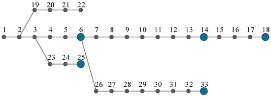
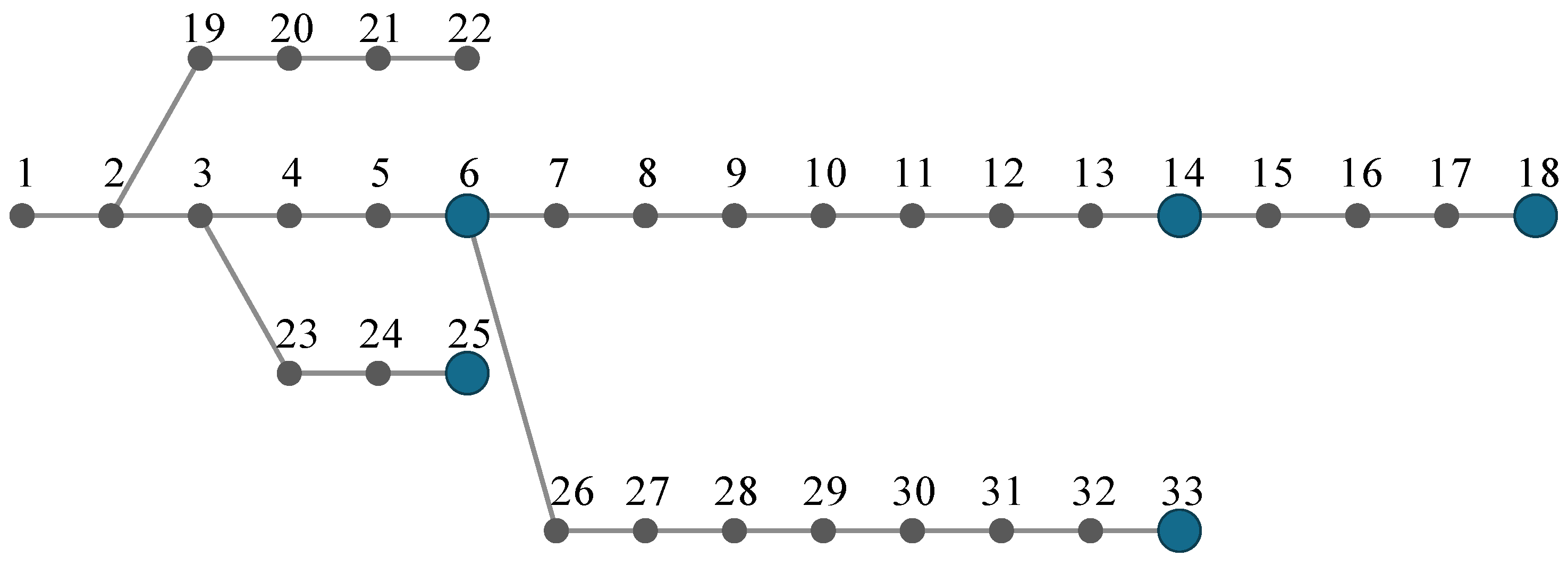
The Baran-Wu 33-bus radial feeder [29] is obtained from the public MATPOWER 8.1 case [30]. Its 32 closed branches are retained and original loads are multiplied by 0.60 to define the study operating point. Figure 1 and Table 3 specify the five resource locations. The locations span the feeder: buses 6 and 14 lie on the main trunk, buses 18 and 33 are the two feeder ends where base voltage is lowest, and bus 25 terminates a lateral, so both voltage and thermal rows are exercised. The assignment of resource types to buses is a study choice, not a siting recommendation. Because calibration is location-independent, moving a resource changes only the network rows: exchanging wind and VPP (wind at bus 25) reduces the area by 3.4% in the baseline and 3.5% in the compound scenario, and exchanging wind and aggregated PV (wind at bus 33) by 8.3% and 8.5%, with delivery failure between 1.65% and 3.10% (Table S5). Because the original case does not provide usable operational thermal ratings, each branch is assigned the larger of 0.55 MVA and 1.4 times its linear base apparent flow. Sixteen of the 32 branches receive the 0.55 MVA floor and sixteen the scaled rating (0.56–3.67 MVA, median 0.56 MVA). Across all boundary commands only three thermal limits bind, on the floor-rated end sections into buses 14, 25 and 33, together with the lower voltage limit at buses 18, 32 and 33; the upper voltage limit never binds. The region boundary is therefore set by a few terminal elements, and its size depends on the assumed 0.55 MVA floor. Linear optimization uses 0.955 to 1.045 p.u.; AC diagnostics use 0.95 to 1.05 p.u. The 0.005 p.u. margin is a preset study parameter, not a statistically certified model-error allowance.

Figure 1. The 33-bus feeder and resource locations. Blue nodes host resources; drawing coordinates represent topology only.

Table 3. Resource command budgets and locations.

Type	Bus	P Budget (MW)	Q Limit (Mvar)
Wind	6	0.90	0.54
PV	14	0.60	0.36
BESS	18	0.50	0.30
VPP	25	0.80	0.48
Aggregated PV	33	0.70	0.42

Without regulation injections, the minimum voltage is 0.95045 p.u. in the linear model and 0.94953 p.u. in AC power flow. The experiment consequently includes corrective undervoltage support: the origin is outside the declaration region under tightened voltage constraints. Declarations cannot all be interpreted as freely withdrawable reserve from an already secure base point. This base-point condition is reported explicitly rather than hiding the corrective requirement within capacity comparisons.

3.2. Synthetic Responses and Data Splits

Table 4 defines the scenario modifications. In Table 3 order, baseline response means are [0.94, 0.95, 0.98, 0.91, 0.93] and standard deviations are [0.025, 0.020, 0.012, 0.035, 0.030], clipped to [0.35, 1]. Ratio noise combines 0.55 times a shared standard normal variable with sqrt(1-0.55 squared) times an independent normal variable. Median activation times are [1.2, 1.0, 0.6, 1.8, 1.5] seconds. Log-time noise is 0.32 times a normal combination with shared and independent coefficients 0.6 and 0.8, reusing the shared variable from response ratios. This generator defines a dependence stress test and is not identified from operational records.

Table 4. Scenario modifications relative to baseline.

Scenario	Response Ratio	Median Time	BESS P Budget
Baseline	unchanged	×1.0	×1.0
Delay	unchanged	×1.8	×1.0
Low SOC	unchanged	×1.0	×0.35
Compound	mean −0.04; SD × 1.5	×1.8	×0.35

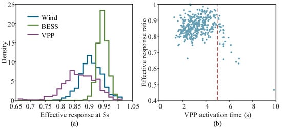
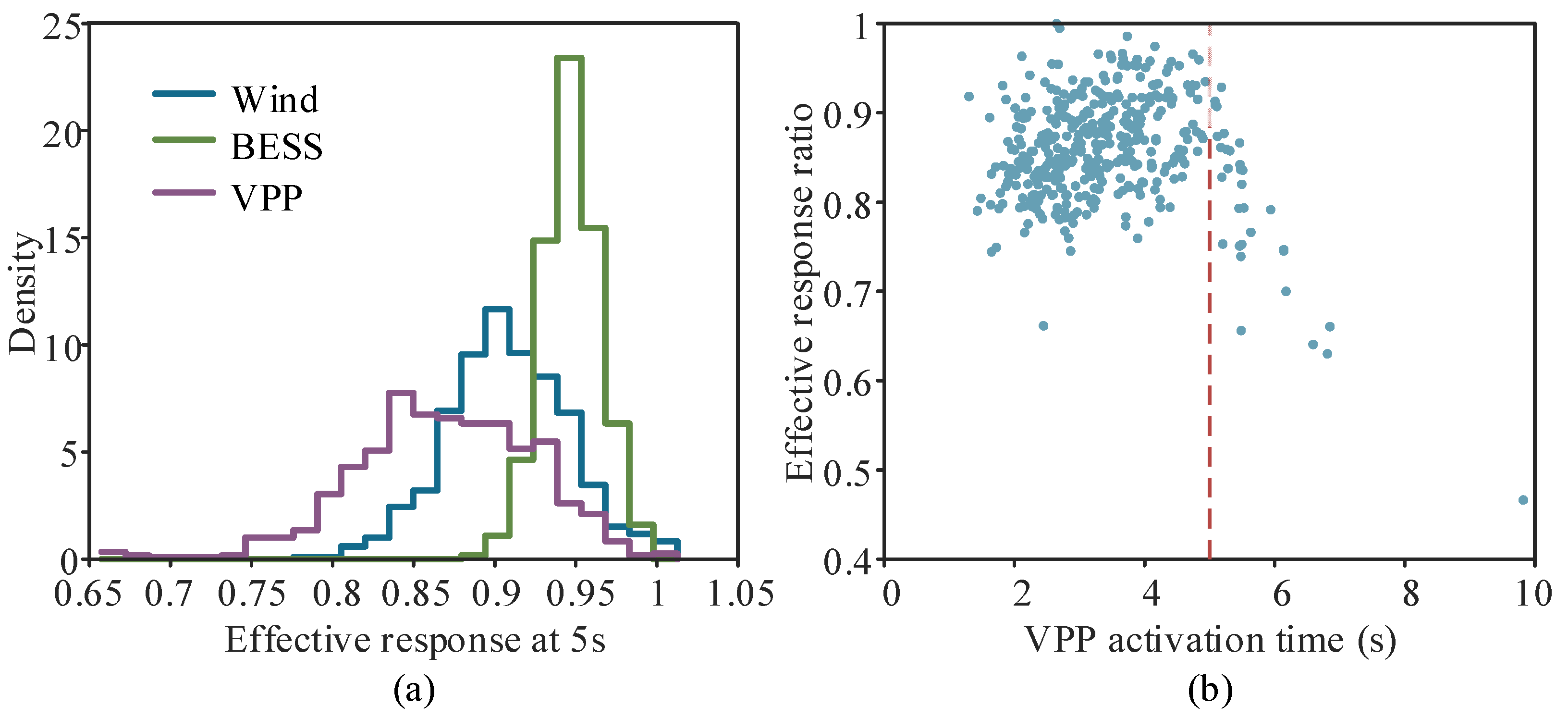
Each scenario has 400 training, 800 calibration and 2000 test joint episodes, totaling 12,800 episodes with five resource responses each. These are not measured dispatch records. The master seed is reproducibility_seed, with distinct seeds across scenarios and splits; arrays are stored in NPZ files. The activation window is five seconds, the main nominal coverage is 0.95 and the boundary sweep uses 72 directions. Figure 2 displays synthetic compound-response distributions and the VPP time-response relation. Bounds are computed from calibration ranks rather than imposed as a single graphical slope.

Figure 2. Empirical response characteristics under the compound scenario: (a) distributions of effective response ratios for wind, BESS, and VPP resources at 5 s; (b) each blue dot represents one synthetic compound-scenario episode, and the red dashed line marks the 5 s activation window.

3.3. Comparators and Evaluation Protocol

Comparators are nominal response β = 1, fixed 0.8 derating, resource-wise empirical 5% quantiles and joint calibration. The 0.8 factor represents a uniform derating: it lies just below the smallest baseline bound (0.83) and inside the compound range of bounds (0.71–0.90), so it exposes both sides of a fixed rule; factors from 0.70 to 0.90 are swept in Table S3. Two further joint-control rules use the same splits: Bonferroni resource-wise conformal bounds at level 1 − (1 − α)/N, and a maximum-shortfall score without standardization. The exact shared-coefficient counterpart of Equation (12) is also evaluated. All comparators share resource budgets, network parameters, test episodes and directions. Nominal response, fixed derating and marginal quantiles are capability-accounting controls, not full reproductions of published algorithms. The no-delay ablation calibrates steady response ratios only; the no-network ablation keeps the same joint bounds while removing network constraints. Every method retains its own declaration-command pairs, avoiding comparisons between contours without implementable allocations.

For each independent test episode, its coefficients are applied to all 72 boundary commands. Any command delivering less P or Q than declared marks one delivery failure. Network failure is counted in the same episode-wise manner, and joint failure is their union in Equation (18). This boundary-wide stress test is stricter than selecting a single random command per episode; the 72 correlated evaluations are not treated as independent samples. Tables report frequencies and 95% Wilson intervals across 2000 independent episodes, quantifying test-frequency uncertainty for a fixed calibration set.

$${\hat{p}}_{\mathrm{j}\mathrm{o}\mathrm{i}\mathrm{n}\mathrm{t}}={\displaystyle \frac{1}{n_{\mathrm{t}\mathrm{e}\mathrm{s}\mathrm{t}}}}{\sum }_k\mathbf{1}\{\exists m: J a_{km}\ngeqq y_m \mathrm{o}\mathrm{r} A a_{km}\nleqq b\}$$

(18)

In Equation (18), J sums the resource active and reactive components separately; failure of a vector inequality means that at least one component violates its bound.

Equation (19) gives the Wilson interval using the relevant test frequency, the 97.5th standard-normal quantile z (approximately 1.96), and 2000 independent test episodes. Delivery, network and union events each use their own frequency. Direction count does not multiply the denominator, and this interval does not prove nominal coverage. Delivery comparisons and network inequalities use a numerical tolerance of 10⁻⁸ in their respective model units, not an operational tracking deadband.

$${\mathrm{C}\mathrm{I}}_{95\%}={\displaystyle \frac{\hat{p}+z^2/(2n_{\mathrm{t}\mathrm{e}\mathrm{s}\mathrm{t}})\pm z\sqrt{\hat{p}(1-\hat{p})/n_{\mathrm{t}\mathrm{e}\mathrm{s}\mathrm{t}}+z^2/(4n_{\mathrm{t}\mathrm{e}\mathrm{s}\mathrm{t}}^2)}}{1+z^2/n_{\mathrm{t}\mathrm{e}\mathrm{s}\mathrm{t}}}}$$

(19)

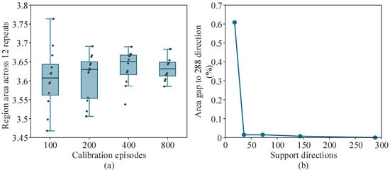
Calibration sizes of 100, 200, 400 and 800 are each repeated 12 times, resampling training and calibration while keeping the test set fixed. Boxplots therefore measure calibration variability without asserting monotone statistical convergence. Direction sweeps use 18, 36, 72, 144 and 288 directions. AC diagnostics apply every one of the 2000 test episodes to all 72 boundary commands, giving 144,000 AC power flows per method and scenario. They are solved by a backward/forward sweep that reproduces the PYPOWER base-case minimum voltage (0.94953 p.u.). With zero unsafe episodes, the one-sided 95% Clopper–Pearson bound on the episode-level violation probability is 0.15%. This bound concerns the stored boundary commands under the synthetic response distribution; the linear guarantee of Equation (17) is not inherited by the AC model.

4. Results and Applicability

4.1. Capacity and Delivery Risk

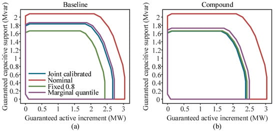
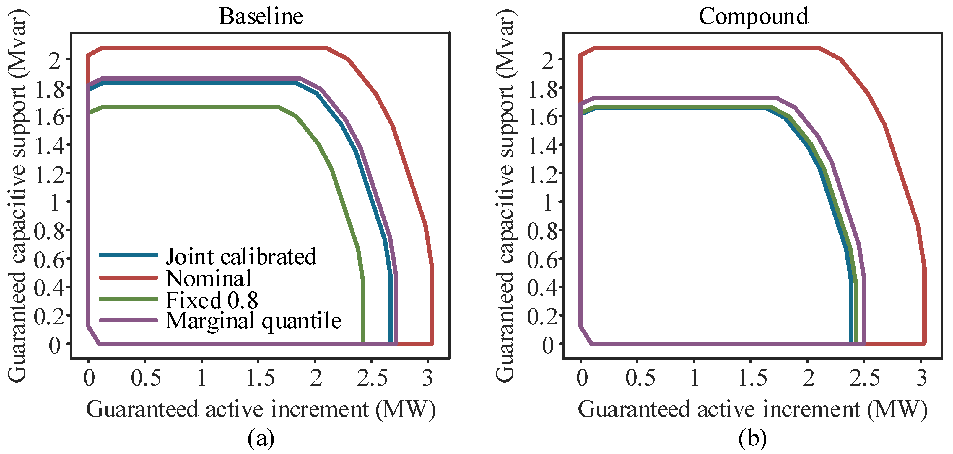
Every boundary in Figure 3 is projected from feasible optimized commands. Joint calibration yields a baseline area of 4.523 MW·Mvar and a compound area of 3.657 MW·Mvar, a 19.15% reduction. Under this generator and operating point, degraded response and reduced BESS headroom reduce declarable capability. One-factor-at-a-time runs with common random numbers attribute the reduction mainly to the response distribution: degraded response ratios alone reduce the area by 15.0%, delay alone by 5.3% and the BESS budget alone by 0.6%; ratios and delay together give 18.7%, and adding the budget cut gives 19.3% (Table S2). The percentage is not an observed reduction in a provincial grid.

Figure 3. Inner regulation regions under representative operating conditions: (a) Baseline scenario; (b) Compound scenario with delayed response and reduced BESS state of charge.

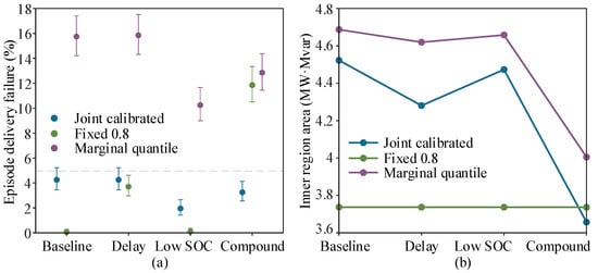
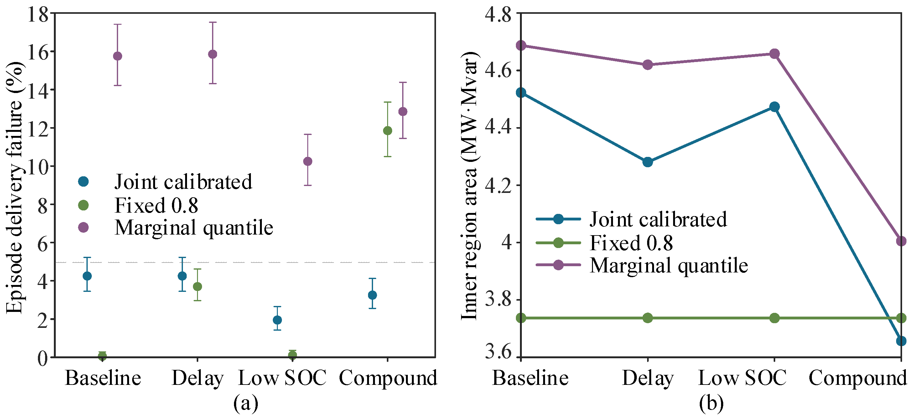
Table 5 reports both delivery and joint failure so that meeting minimum response is not conflated with network safety. Figure 4 shows the two-sided behavior of fixed derating: it withholds area in baseline conditions but can be optimistic under compound stress. Marginal resource-wise quantiles permit larger regions without controlling the joint tail event. Nominal response almost inevitably fails strict boundary delivery here because the generator enforces ρ ≤ 1 and declarations have zero tolerance. This is a structural control, not evidence of a universal improvement over practical dispatch policies.

Table 5. Joint-calibrated capability and episode failure by scenario.

Scenario	Max P (MW)	Area (MW·Mvar)	Delivery % [95% CI]	Joint % [95% CI]
Baseline	2.670	4.523	4.25 [3.45, 5.23]	4.70 [3.86, 5.72]
Delay	2.595	4.281	4.25 [3.45, 5.23]	4.60 [3.77, 5.61]
Low SOC	2.645	4.473	1.95 [1.43, 2.65]	2.50 [1.90, 3.28]
Compound	2.388	3.657	3.25 [2.56, 4.12]	3.60 [2.87, 4.51]

Figure 4. Reliability and usable region size across operating scenarios: (a) episode delivery failure rate with 95% confidence intervals; (b) corresponding inner regulation region area.

Table S1 varies the generator. With response standard deviations scaled by 0.5–3 and the shared coefficient between 0 and 0.95, joint-calibrated delivery failure stays between 1.30% and 4.85%, while the area falls from 4.86 to 3.29 MW·Mvar. Fixed 0.8 derating keeps a constant area of 3.74 MW·Mvar; its failure is below 0.2% up to the baseline dispersion, about 5% at twice and 14% at three times that dispersion. Joint calibration therefore returns capability when responses are tight and removes it when they are dispersed. Stronger correlation enlarges the joint region at a given dispersion because the maximum score is less penalized. Scaling median activation time by 1–2.6 and log-time dispersion from 0.16 to 0.48 leaves joint failure at 2.75–3.90% but raises fixed-derating failure to 38.95%. Failure is binary because the coverage statement concerns an event. Its magnitude is small under matched calibration: in failing episodes the mean worst-case active shortfall is 1.0–4.4 kW and the largest is 106 kW, compared with 18.4 kW and 282 kW under the mismatch of Section 4.4 (Table S4). An economic assessment would multiply expected shortfall by a penalty price and would require controlling that loss directly [26].

4.2. Coverage Levels and Ablations

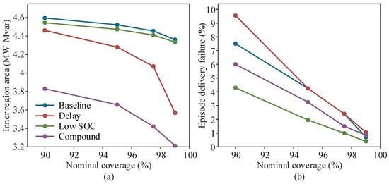
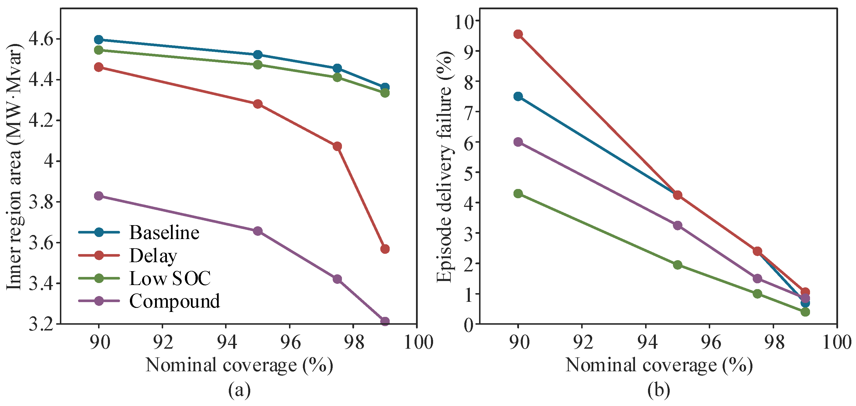
Figure 5 changes nominal coverage while holding data splits fixed. Increasing α raises the rank threshold and lowers β. In this construction, a high-coverage declaration can also be implemented at lower coverage by reducing commands appropriately, giving an interpretation in terms of nested exact sets. Plotted areas nevertheless come from fresh solves, and finite-direction area trends are not a proof of statistical coverage. Held-out frequencies may fluctuate and need not equal the nominal failure level.

Figure 5. Sensitivity of the calibrated inner region to nominal coverage level: (a) variation of inner region area; (b) variation of episode delivery failure rate.

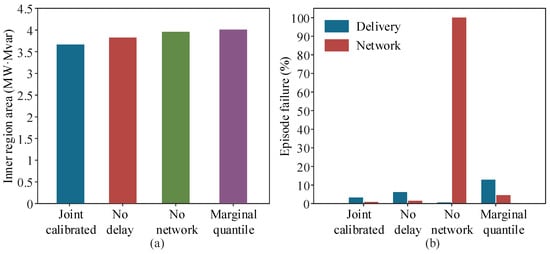
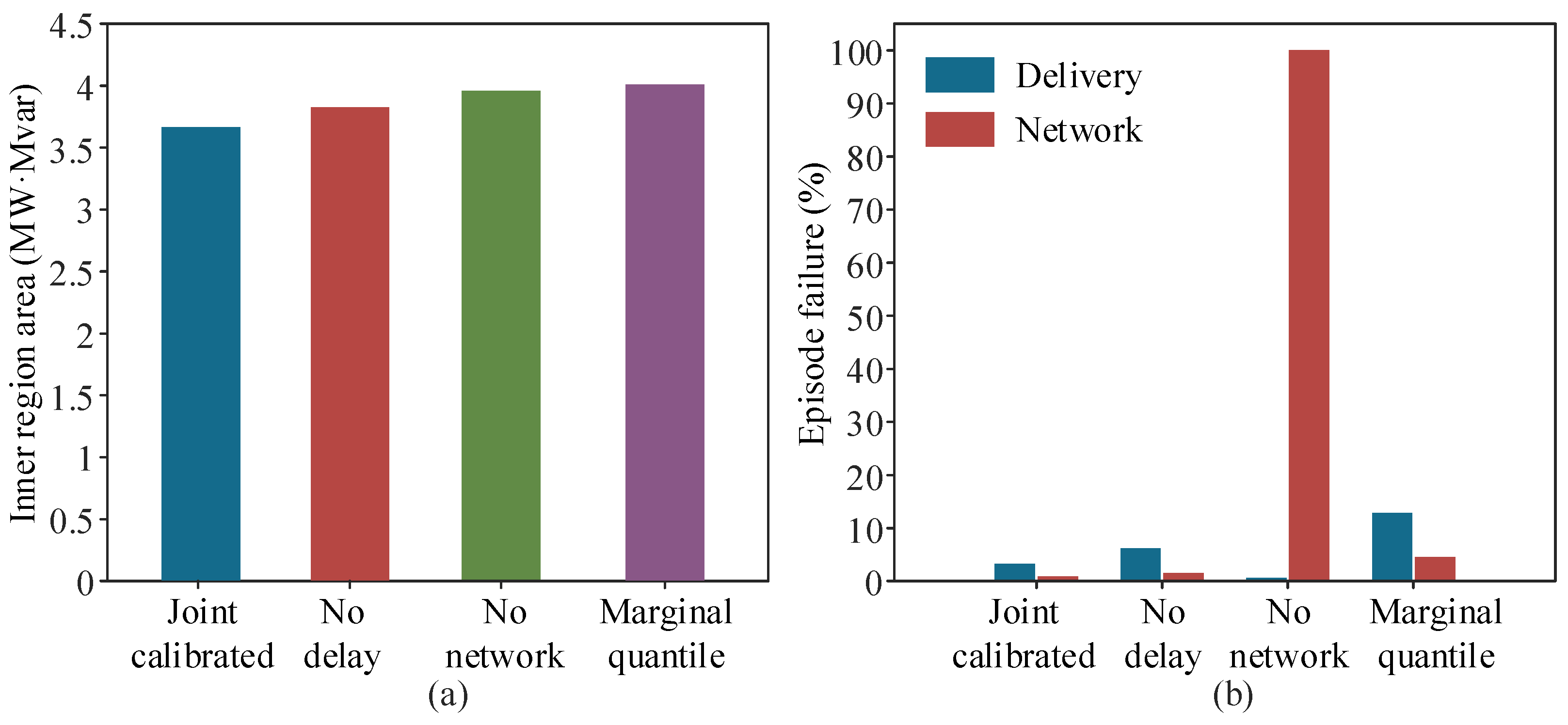
Table 6 and Figure 6 show 6.20% compound delivery failure without delay calibration, versus 3.25% with joint calibration. The no-network row is a definitional check: its commands are optimized without network limits, so linear violations in every episode are expected. The informative comparison is the nominal row, which respects network limits but ignores delivery uncertainty. Its network rows are satisfied only at full response; because the base point needs corrective voltage support, under-delivery leaves the tightened lower voltage limit violated in every episode. Delivery failure can decrease after removing the network because the optimized allocation changes. Delivery and network mechanisms must therefore be interpreted separately instead of forcing a single-metric ranking.

Table 6. Compound-scenario controls and ablations.

Method	Area (MW·Mvar)	Delivery (%)	Network (%)	Joint (%)
Joint calibrated	3.657	3.25	0.90	3.60
Nominal	5.843	100.00	100.00	100.00
Fixed 0.8	3.737	11.85	0.55	12.30
Marginal quantile	4.005	12.85	4.50	14.60
No delay	3.821	6.20	1.50	7.00
No network	3.951	0.60	100.00	100.00
Shared P/Q counterpart	3.657	3.25	0.90	3.60
Bonferroni conformal	3.536	2.50	0.50	2.70
Unscaled maximum score	3.610	4.35	0.45	4.75
Fixed 0.75	3.283	4.10	0.15	4.25

Figure 6. Ablation analysis under the compound scenario: (a) inner region area obtained by different modeling variants; (b) delivery and network failure rates of the corresponding variants.

The exact shared-coefficient counterpart enlarges the area by only 0.007–0.013% across the four scenarios, because the voltage rows are identical under both sets and only mixed-sign thermal facets differ; the componentwise box therefore withholds a negligible share of capability here, at the cost of 2890 auxiliary variables for the exact form. Among the three rules with joint control, the standardized maximum score gives the largest area: 3.4% above Bonferroni and 1.3% above the unscaled score in the compound scenario (1.0% and 1.3% in the baseline), with all three below 5% delivery failure. No fixed factor matches it in both scenarios: 0.85 gives 4.40% failure in the baseline but 40.30% under compound stress, whereas 0.75 holds 4.10% under compound stress but withholds 27% of the baseline area (Table S3).

4.3. Numerical Stability and AC Diagnostics

The left panel of Figure 7 shows area distributions from 12 independent calibrations per sample size, retaining random variation. The right panel reports actual direction refinement. The 72-direction area differs from the 288-direction reference by 0.0148%; the measured 72-direction sweep takes approximately 0.219 s. This single-machine timing excludes generation, Monte Carlo evaluation, document building and AC checks, and is not a production real-time guarantee. Maximum primal inequality residuals are below 10⁻⁷. An independent check enumerates all 1024 box vertices for sampled boundary commands.

Figure 7. Numerical stability and directional discretization effects: (a) boxes show the interquartile range with the median line, whiskers show the range, and black dots denote the 12 individual runs; (b) area gap relative to the 288-direction benchmark.

Across repeated calibrations, joint response-box noncoverage ranges from 2.20% to 8.00% with 100 calibration episodes and from 3.65% to 5.85% with 800. These are box-event failures, not the declaration-delivery failures in Table 5. Because repeats share a fixed test set, the ranges describe calibration variability and are not confidence intervals from independent repeated test populations.

All AC power flows converge (Table 7). For the joint-calibrated region no episode contains a voltage or thermal violation in any of the four scenarios (576,000 flows; Table S6). The lowest voltage is 0.9536 p.u., leaving 0.0036 p.u. to the 0.95 limit, and the highest is 1.0392 p.u. Loading reaches 100.0% only on terminal sections, where the receiving-end flow equals the resource-bus injection and the linear limit is exact. The linear model overestimates voltage by at most 0.00116 p.u., which the 0.005 p.u. margin absorbs; evaluated against the tightened 0.955 p.u. limit itself, the AC voltage of at least one boundary command falls below it in every episode. The linear guarantee is thus not inherited by the AC model, and AC compliance here rests on the preset margin. Nominal commands are AC-safe but fail delivery, which separates the two risks. Zero observed violations bound the violation probability of the stored boundary commands at 0.15%; they do not certify interior points, other feeders or dynamic security. At the substation, the AC active-power relief exceeds the resource-side sum by 0.005–0.060 MW for every boundary command and episode because losses fall, so resource-side active declarations are conservative at the PCC in this benchmark; this ordering is not guaranteed for feeders with reverse flow.

Table 7. Full-boundary AC power-flow diagnostics in the compound scenario.

Method	Unsafe Episodes/2000	95% Upper Bound (%)	Min Voltage (p.u.)	Max Voltage (p.u.)	Max Loading (%)	Max Voltage Error (p.u.)
Joint calibrated	0	0.15	0.9539	1.0329	100.0	0.00113
Nominal	0	0.15	0.9535	1.0314	100.0	0.00113
No network	2000	–	0.9495	1.0408	125.0	0.00125

4.4. Distribution Mismatch and Deployment Conditions

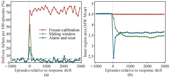
Applying baseline-calibrated bounds to compound responses, with commands re-solved under compound budgets, raises delivery failure to 71.55% and joint failure to 83.45%. This breaks exchangeability and is not a counterexample to conformal coverage, but it is the main practical limitation of the method: the guarantee says nothing once the response distribution moves; the failure is not graceful, and the offline procedure gives no warning. Two simple remedies are therefore tested on a stream of 1000 baseline episodes followed by 3000 compound episodes, with bounds updated every 25 episodes (Figure 8). A sliding window keeps the latest 800 calibration episodes with fixed training statistics. An alarm-and-reset rule monitors the calibrated score itself: under exchangeability, at most 5% of episodes exceed $q_{\mathsf{\alpha }}$, and nine or more exceedances within the last 50 episodes (probability below 0.1% per window) raise an alarm. Calibration data are then discarded, declarations are withheld until the new rank is finite, and training and calibration sets are regrown from post-alarm episodes.

Figure 8. The vertical gray dotted line marks the response shift, and the horizontal dashed line marks the 5% nominal level: (a) delivery failure per 100 episodes under frozen calibration, a sliding calibration window and alarm-and-reset recalibration; (b) corresponding inner region area. The dashed line marks the 5% nominal level.

Frozen calibration fails in 72.9% of post-shift episodes. The sliding window fails in 52% of the first 100 episodes and 5.75% of the next 400, then settles at 1.7% with an area of 3.43 MW·Mvar; it is conservative because the standardization is stale. The alarm fires at the first update after the shift, with no false alarm in the 1000 preceding episodes. Failure is 21% in the first 100 episodes, mostly incurred before the alarm, then 3.5% over the next 400 and about 3% thereafter, and the area returns to 3.62 MW·Mvar, close to the matched-calibration value of 3.657. The alarm requires only quantities already computed, so it can run in real time. Neither scheme has a finite-sample guarantee during the transition, and only one abrupt shift is tested; gradual drift, recurring regimes and repeated-testing control of the alarm remain open.

These schemes are not implementations of weighted conformal inference for non-exchangeable data [24] or adaptive online conformal inference [25], nor of out-of-distribution-aware retraining [23]. A fair comparison with them would need the same episode-level joint event rather than a per-step forecast interval, the same stream and update frequency, and the region re-solved at every update so that capability as well as coverage is compared. Better resource-level forecasts, for example from pretrained large models for distributed PV [31], could narrow the response bounds entering the calibration step, but they are outside the present scope. Controlling shortfall magnitude or economic loss would require a loss-based formulation [26].

Relative to dispatchable-region, stochastic-flexibility and operating-envelope work [3,4,5,6,7,8,9,10,11], the testable addition is the explicit link from a joint timely-response event to a declaration with recoverable commands, with delivery and network risk separated on the same held-out episodes. The study does not establish superiority over all existing stochastic or robust algorithms. Current controls isolate calibration rules and constraint modules. Stronger algorithmic superiority claims would require full recent-method reproductions under aligned risk definitions, information and computational budgets. The added comparators (Bonferroni and unscaled joint rules, the shared-coefficient counterpart and a derating sweep) share the risk definition and data; probabilistic aggregation [12] and finite-covering boundaries [13] define risk on different events and are not reproduced.

Several boundaries remain: one public feeder, fixed demand and topology, one activation window and quadrant, a shared P/Q response coefficient, assumed renewable headroom, and no fault transients, system strength, AGC closed loop or intertemporal SOC. Multiple activation windows could use a time-indexed score, the maximum standardized shortfall over resources and windows within one service episode, which gives simultaneous bounds for all windows by the same rank argument; SOC and energy limits would enter as deterministic linear constraints coupling the commands, and the region would become a projection of a higher-dimensional polytope. The method has not been tested on an unbalanced three-phase feeder. Calibration is unaffected by phasing, and Equation (11) applies to any linear network model with nonnegative commands, including linearized three-phase models used for operating envelopes [5,16], but the results reported here do not transfer without such a test. The results support interpretation of declaration reliability and a reproducible methodological baseline. They do not establish provincial reserve-procurement savings, frequency security or universal dispatch credibility.

5. Conclusions

Joint response calibration and robust linear network constraints produce an inner regulation region with recoverable commands. Finite-sample coverage requires exchangeable episodes. In this synthetic benchmark, fixed derating is conservative in baseline conditions but optimistic under compound stress; marginal quantiles do not provide joint coverage. Capability area must therefore be interpreted together with delivery and network failures.

Distribution mismatch sharply degrades delivery; in the tested abrupt shift, an alarm on the calibrated score followed by recalibration restores failure to about 3% after a short transition. Full-boundary AC checks show no violation, but AC compliance rests on a preset voltage margin and not on the linear guarantee. Sensitivity sweeps indicate that joint calibration is most useful when response dispersion or activation time differs from what a fixed derating factor implicitly assumes.

References

- IEEE Std 2800-2022; IEEE Standard for Interconnection and Interoperability of Inverter-Based Resources (IBRs) Interconnecting with Associated Transmission Electric Power Systems. IEEE: New York, NY, USA, 2022.
- Wei, W.; Liu, F.; Mei, S. Dispatchable Region of the Variable Wind Generation. IEEE Trans. Power Syst. 2015, 30, 2755–2765. [Google Scholar] [CrossRef] [Scilit]
- Liu, Y.; Li, Z.; Wei, W.; Zheng, J.H.; Zhang, H. Data-Driven Dispatchable Regions with Potentially Active Boundaries for Renewable Power Generation: Concept and Construction. IEEE Trans. Sustain. Energy 2022, 13, 882–891. [Google Scholar] [CrossRef] [Scilit]
- Li, Z.; Huang, W.; Zheng, J.H.; Wu, Q.H. Dispatchable Region for Active Distribution Networks Using Approximate Second-Order Cone Relaxation. CSEE J. Power Energy Syst. 2023, 9, 1999–2007. [Google Scholar] [CrossRef] [Scilit]
- Liu, B.; Braslavsky, J.H. Robust Dynamic Operating Envelopes for DER Integration in Unbalanced Distribution Networks. IEEE Trans. Power Syst. 2024, 39, 3921–3936. [Google Scholar] [CrossRef] [Scilit]
- Wen, Y.; Hu, Z.; Liu, L. Aggregate Temporally Coupled Power Flexibility of DERs Considering Distribution System Security Constraints. IEEE Trans. Power Syst. 2023, 38, 3884–3896. [Google Scholar] [CrossRef] [Scilit]
- Wang, S.; Wu, W.; Chen, Q.; Yu, J.; Wang, P. Stochastic Flexibility Evaluation for Virtual Power Plants by Aggregating Distributed Energy Resources. CSEE J. Power Energy Syst. 2024, 10, 988–999. [Google Scholar] [CrossRef] [Scilit]
- Wen, Y.; Guo, Y.; Hu, Z.; Hug, G. Stochastic modeling for the aggregated flexibility of distributed energy resources. Electr. Power Syst. Res. 2024, 234, 110628. [Google Scholar] [CrossRef] [Scilit]
- Fang, F.; Yu, S.; Xin, X. Data-Driven-Based Stochastic Robust Optimization for a Virtual Power Plant with Multiple Uncertainties. IEEE Trans. Power Syst. 2022, 37, 456–466. [Google Scholar] [CrossRef] [Scilit]
- Patig, A.; Stanojev, O.; Aristidou, P.; Kiprakis, A.; Hug, G. Fast Mapping of Flexibility Regions at TSO-DSO Interfaces under Uncertainty. In Proceedings of the 2022 IEEE PES Innovative Smart Grid Technologies Conference Europe (ISGT-Europe), Novi Sad, Serbia, 10–12 October 2022; pp. 1–6. [Google Scholar] [CrossRef] [Scilit]
- Kar, A.S.; Challa, K.K.; Bharati, A.K.; Singhal, A.; Ajjarapu, V. Robust VAR Capability Curve of DER with Uncertain Renewable Generation. In Proceedings of the 2024 IEEE Power & Energy Society General Meeting (PESGM), Seattle, WA, USA, 21–25 July 2024; pp. 1–5. [Google Scholar] [CrossRef] [Scilit]
- Jacobs, M.; Paolone, M. Probabilistic Flexibility Aggregation of DERs for Ancillary Services Provision. IEEE Trans. Power Syst. 2026, 41, 3965–3978. [Google Scholar] [CrossRef] [Scilit]
- Xie, H.; Zhao, X.; Gao, S.; Zhang, N.; Li, Q. Finite-covering-based hierarchical robust flexibility and uncertainty boundary estimation for aggregated distributed energy resources. Int. J. Electr. Power Energy Syst. 2026, 176, 111771. [Google Scholar] [CrossRef] [Scilit]
- Angelopoulos, A.N.; Bates, S. Conformal Prediction: A Gentle Introduction. Found. Trends Mach. Learn. 2023, 16, 494–591. [Google Scholar] [CrossRef] [Scilit]
- Rousseau, J.; Cai, H.; Heer, P.; Orehounig, K.; Hug, G. Uncertainty-Aware Flexibility of HVAC Systems in Buildings: From Quantification to Provision. IEEE Trans. Smart Grid 2026, 17, 269–282. [Google Scholar] [CrossRef] [Scilit]
- Liu, B.; Braslavsky, J.H. Sensitivity and Robustness Issues of Operating Envelopes in Unbalanced Distribution Networks. IEEE Access 2022, 10, 92789–92798. [Google Scholar] [CrossRef] [Scilit]
- Liu, B.; Braslavsky, J.H. Robust Dynamic Operating Envelopes via Superellipsoid-Based Convex Optimisation in Unbalanced Distribution Networks. IEEE Trans. Power Syst. 2024, 39, 4775–4778. [Google Scholar] [CrossRef] [Scilit]
- Liu, B.; Braslavsky, J.H. Computation of Robust Dynamic Operating Envelopes Based on Non-convex OPF for Unbalanced Distribution Networks. arXiv 2024, arXiv:2404.03355. [Google Scholar] [CrossRef] [Scilit]
- Pozo, D. TSO-DSO Flexibility Regions are Non-Convex. IEEE Trans. Power Syst. 2025, 40, 5480–5482. [Google Scholar] [CrossRef] [Scilit]
- Prionistis, G.; Vournas, C. Flexibility region discontinuity due to overvoltage constraints. Sustain. Energy Grids Netw. 2025, 43, 101807. [Google Scholar] [CrossRef] [Scilit]
- Schlembach, F.; Smirnov, E.; Koprinska, I.; Winands, M.H.M. Conformal multistep-ahead multivariate time-series forecasting. Mach. Learn. 2025, 114, 165. [Google Scholar] [CrossRef] [Scilit]
- Nam, N.B.; Ogliari, E.; Leva, S.; Pafumi, E.; Alberti, D.; Duong, M.Q. Comparative analysis of conformal prediction techniques and machine learning models for very short-term solar power forecasting. Energy AI 2025, 21, 100573. [Google Scholar] [CrossRef] [Scilit]
- Ilić, U.; Kundačina, O.; Petrušić, A.; Andrejević Stošović, M.; Radivojević, N.; Stajić, Z. Out-of-Distribution-Aware Time Series Conformal Prediction with Adaptive Retraining for Solar Power Forecasting. Energies 2026, 19, 3446. [Google Scholar] [CrossRef] [Scilit]
- Barber, R.F.; Candès, E.J.; Ramdas, A.; Tibshirani, R.J. Conformal prediction beyond exchangeability. Ann. Stat. 2023, 51, 816–845. [Google Scholar] [CrossRef] [Scilit]
- Gibbs, I.; Candes, E.J. Conformal Inference for Online Prediction with Arbitrary Distribution Shifts. J. Mach. Learn. Res. 2024, 25, 1–36. [Google Scholar]
- Angelopoulos, A.N.; Bates, S.; Fisch, A.; Lei, L.; Schuster, T. Conformal Risk Control. International Conference on Learning Representations; 2024. Available online: https://proceedings.iclr.cc/paper_files/paper/2024/hash/f3549ef9b5ff520a7e41ff3cc306ab2b-Abstract-Conference.html (accessed on 6 September 2026).
- Virtanen, P.; Gommers, R.; Oliphant, T.E.; Haberland, M.; Reddy, T.; Cournapeau, D. SciPy 1.0: Fundamental algorithms for scientific computing in Python. Nat. Methods 2020, 17, 261–272. [Google Scholar] [CrossRef] [Scilit] [PubMed]
- Huangfu, Q.; Hall, J.A.J. Parallelizing the dual revised simplex method. Math. Program. Comput. 2018, 10, 119–142. [Google Scholar] [CrossRef] [Scilit]
- Baran, M.E.; Wu, F.F. Network reconfiguration in distribution systems for loss reduction and load balancing. IEEE Trans. Power Deliv. 1989, 4, 1401–1407. [Google Scholar] [CrossRef] [Scilit]
- Zimmerman, R.D.; Murillo-Sanchez, C.E.; Thomas, R.J. MATPOWER: Steady-State Operations, Planning, and Analysis Tools for Power Systems Research and Education. IEEE Trans. Power Syst. 2011, 26, 12–19. [Google Scholar] [CrossRef] [Scilit]
- Gao, M.; Zhou, S.; Gu, W.; Fan, J.; Liu, H.; Guan, A.; Xu, H. Pre-Trained Large Model as Distributed PV Power Forecaster: Integrating Scenario-Consistent Retrieval-Augmented Generation and Cross-Modal Semantic Alignment. IEEE Trans. Sustain. Energy 2026, 17, 2394–2407. [Google Scholar] [CrossRef] [Scilit]
Disclaimer/Publisher’s Note: The statements, opinions and data contained in all publications are solely those of the individual author(s) and contributor(s) and not of MDPI and/or the editor(s). MDPI and/or the editor(s) disclaim responsibility for any injury to people or property resulting from any ideas, methods, instructions or products referred to in the content. |
© 2026 by the authors. Licensee MDPI, Basel, Switzerland. This article is an open access article distributed under the terms and conditions of the Creative Commons Attribution (CC BY) license.