


Abstract
Over the next few years, prediction of biogas production using machine learning techniques at municipal wastewater treatment plants may become an indispensable tool for ensuring the energy self-sufficiency of such facilities. The objective of this study was to develop and compare predictive models capable of estimating energy management indicators for a wastewater treatment plant based on technological and physicochemical parameters for the wastewater treatment plant in Iława (Poland). In the first stage, the process parameters were subjected to principal component analysis (PCA). Next, predictive models were built based on four approaches: a multilayer perceptron (MLP), a random forest, support vector regression (SVR), and the XGBoost algorithm, and their predictive capabilities were compared using test data. The results of the study showed that a multilayer neural network allows for very accurate modeling of selected energy factors related to the operation of a wastewater treatment plant. The use of model optimization techniques—cross-validation (base models) and hyperparameter tuning (neural network)—provide evidence that the multilayer neural network has the greatest potential for accurate and reliable prediction, with a final performance result of R2 = 0.9752 for biogas production.
1. Introduction
The growing demand for energy and the depletion of conventional resources are drawing increasing attention to the generation of energy from renewable sources and to improving the energy efficiency of available technologies. This issue also affects water and wastewater treatment facilities [1]. It is estimated that the water and wastewater sector accounts for nearly 40% of total electricity consumption in cities [2].
Wastewater treatment plants (WWTPs) face an increasing volume of wastewater, stricter environmental regulations, and public pressure to implement more sustainable and energy-efficient waste management strategies [3]. WWTPs are energy-intensive facilities that account for significant greenhouse gas emissions and incur high operating costs. Therefore, improving process efficiency can yield broad environmental and economic benefits [4].
Currently, anaerobic digestion (AD) is widely used at many wastewater treatment plants for the management of sewage sludge, thereby contributing to energy self-sufficiency. On average, the facilities using AD consume 40% less net energy compared to WWTPs without this technology [5]. AD enables both the production of biogas, which can be used to generate electricity and heat, and the recovery of raw materials [6]. AD is a multi-stage process in which diverse groups of microorganisms are used for the anaerobic decomposition of organic compounds, and these microorganisms require appropriate process conditions [7]. Despite the many benefits of this technology, the main challenge is its sensitivity to changes in sludge composition, the presence of toxic substances, and fluctuations in operating parameters, which can lead to a breakdown in process stability. For this reason, anaerobic digestion of sewage sludge often exhibits poor efficiency, characterized by low methane yield (typically below 50% of theoretical potential) and prolonged fermentation time (approximately 20 days). These limitations significantly hinder the efficient recovery and utilization of biomass energy from sewage sludge [8]. With this in mind, there is an ongoing search for new, advanced methods to predict and optimize key operational parameters of the process.
The mechanistic models used to date, such as Anaerobic Digestion Model No. 1 (ADM1), require knowledge of many variables—for example, detailed data on the concentrations of individual substrates—as well as specialized, expensive software and trained personnel. For this reason, their application in facilities operating on an industrial scale is limited [7,9].
In recent years, models utilizing machine learning techniques have gained increasing attention. They offer an alternative to mechanistic models, particularly in areas requiring the improvement of existing solutions, in highly variable environments, and when insights need to be derived from large datasets [7,10]. Previous research on machine learning methods for predicting biogas production at wastewater treatment plants has shown that neural networks are potentially the most effective model [11]. At the same time, it has been noted that their limitation is the need for high computational power. It should also be noted that research on biogas production prediction using neural networks has focused almost exclusively on the models with a single hidden layer [12]; in this study, the authors decided to investigate the potential of multilayer models. Sadoune et al. [13], using Bayesian optimization and various types of standardization, achieved biogas production prediction results with an R2 of 0.712 from only 16 input variables, which encourages the use of deep learning methods while leaving considerable room for improvement. In contrast, in a study conducted by Lucas et al. [14] on predicting methane concentration in biogas produced at a wastewater treatment plant, deep learning models were used in the context of time series analysis; the present study focused on predictions based on other plant operating parameters, rather than on predicting values over time, which is also described in other works of members of research team [15]. Simple predictive tools for simulating or forecasting the amount of biogas produced at wastewater treatment plants are also known and available [16,17].
The objective of this study was to develop and thoroughly compare predictive models that enable the estimation of energy management indicators for wastewater treatment plants based on routinely recorded technological and physicochemical parameters of the wastewater treatment process and sewage sludge treatment. In the first stage, the process parameters were subjected to principal component analysis (PCA), and then an assessment was made of which energy indicators could be reliably modeled in this reduced feature space. Next, predictive models were built based on four approaches: a multilayer perceptron (MLP), a random forest (random forest), support vector regression (SVR), and the XGBoost algorithm, and their predictive capabilities were compared using test data—i.e., data not used in the training process. In the first phase of the comparison, the multilayer neural network already demonstrated an advantage over traditional machine learning models. Subsequently, model optimization using Bayesian search—which additionally incorporated a dropout mechanism and objective function regularization—further improved the neural network’s performance and strengthened the model’s resilience to potential overfitting with a final result of performance with R2 = 0.9752 for biogas production. It should be noted that, to date, no studies have been carried out on forecasting biogas production using deep neural networks based on actual operating parameters and physicochemical indicators across such a wide range.
2. Materials and Methods
2.1. Source Data and Their Preliminary Processing
The source data used to develop predictive models were obtained from a wastewater treatment plant located in Iława (Poland). The WWTP was designed for an average daily flow of 26,940 m3/d and a population equivalent of 154,117. In addition to municipal wastewater, the plant also receives wastewater from a slaughterhouse and poultry processing plant, a pulp mill, and a potato processing plant. It employs two treatment stages: mechanical and biological. In the first stage, the wastewater is directed to screens, then passes through sand traps, grease separators, and primary settling tanks. Biological treatment takes place in nitrification and denitrification chambers, as well as in separate biological dephosphatation chambers. The final component of this stage is the secondary settling tanks. In turn, the following equipment is used for sewage sludge treatment: gravity thickeners, drum thickeners, closed, separate fermentation chambers, a decanting centrifuge, and a solar sludge dryer. Methane fermentation conducted under mesophilic conditions at a temperature of 37–39 °C, with an average hydraulic retention time of 37 days, is used to stabilize the sewage sludge. The biogas produced is stored in a biogas tank and used in Combined Heat and Power (CHP) units to generate electricity and heat. At the WWTP in Iława, a co-substrate in the form of byproducts from poultry processing is added to the sewage sludge.
The raw dataset included 57 variables characterizing the facility operations, compiled for 36 consecutive months, from January 2017 to December 2019. For the presented parameters, daily values were obtained from technologist of a wastewater treatment plant, and these were used to calculate the average values for each month. The observation from April 2017 was excluded from further analysis due to missing data, and the variable with zero variance—dry matter content in the co-fermenter—was removed. Two groups were identified from the remaining variables. The first group consisted of 41 technological and physicochemical parameters characterizing the wastewater treatment process, while the second group comprised 15 indicators related to the treatment plant’s energy management, including, among others, biogas production and energy production and consumption.
In further modeling, the technological and physicochemical parameters were treated as potential explanatory variables, while the energy indicators were treated as potential response variables. Variables expressed as percentages were subjected to a logarithmic transformation
x′ = −ln(x).
Subsequently, for the purposes of model development and evaluation, the 35 observations were divided in an 80:20 ratio into a training set covering the first 28 months and a test set covering the remaining 7 months.
2.2. Principal Component Analysis
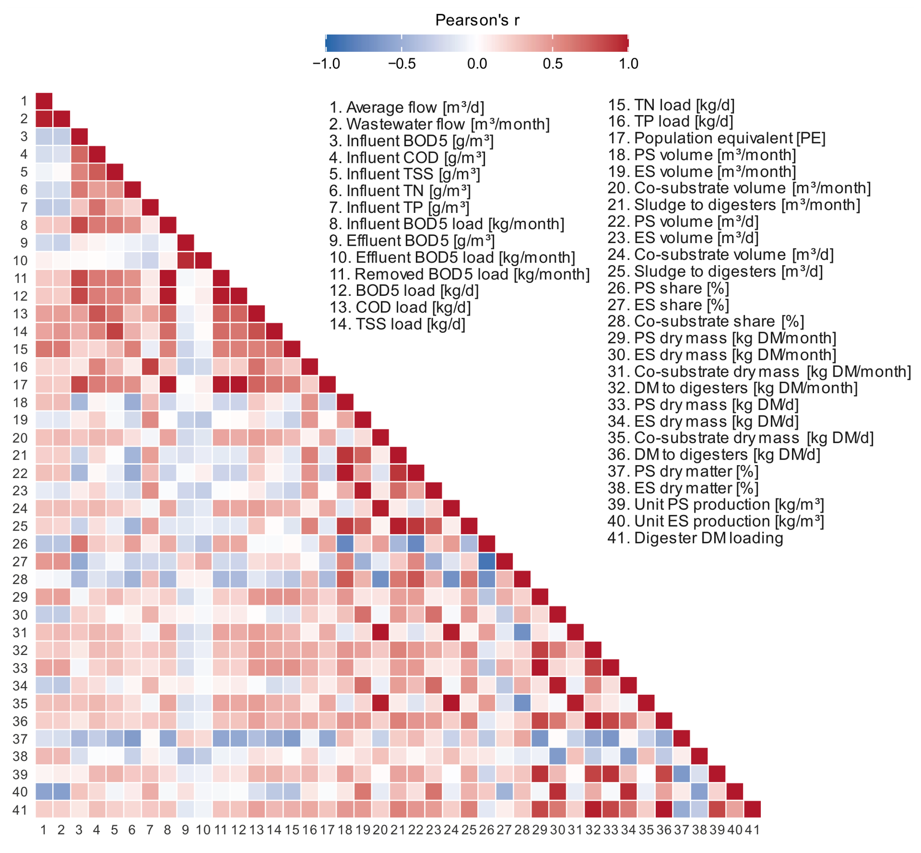
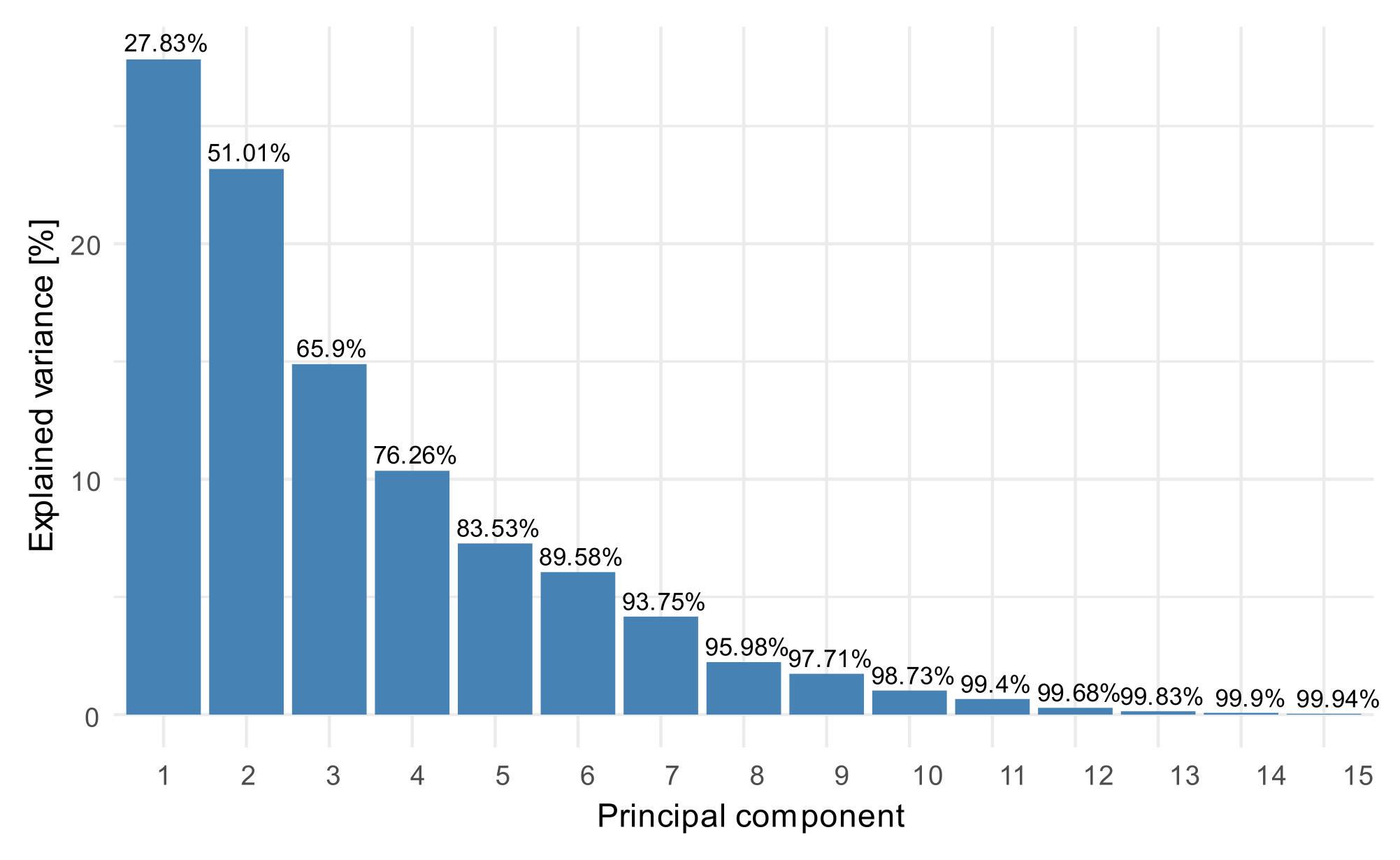
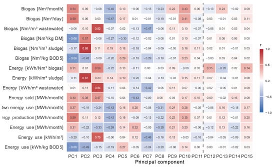
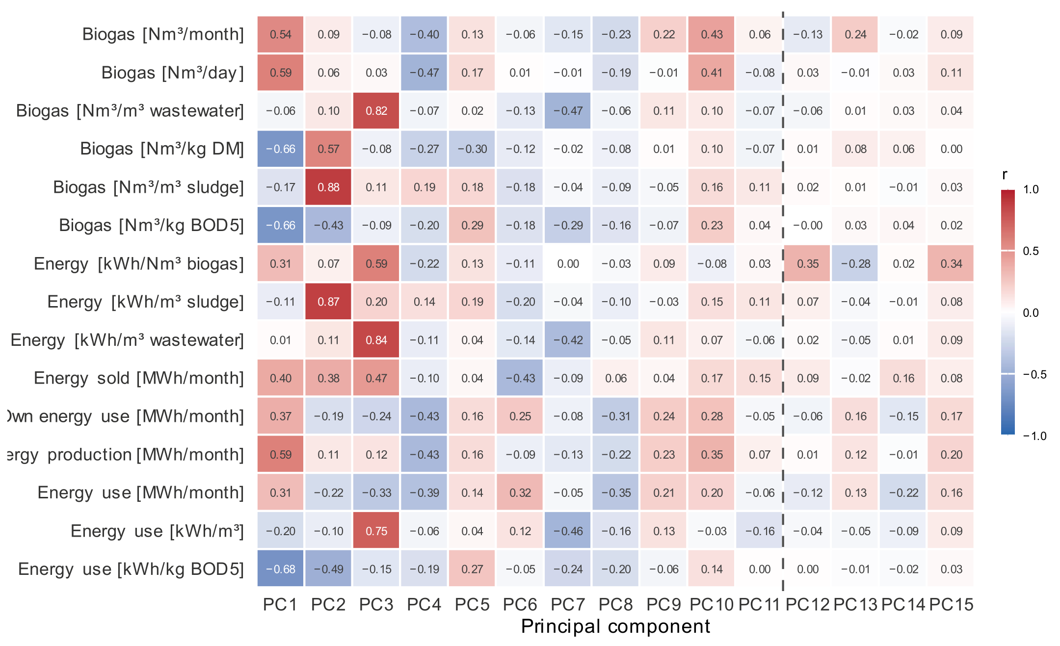
Due to the large number of input variables, particularly relative to the number of cases, it was decided that predictors needed to be preselected for further analysis. Since the dataset contains many variables that are derived from one another and high correlations involving more than two variables (see Figure 1), it was determined that, rather than a direct, arbitrary selection of variables, using a mathematically well-established method of dimensionality reduction would be a superior approach. For this purpose, the well-known PCA method was used, which allowed for the statistical combination of highly correlated variables into a set of new factors that remained orthogonal to one another. PCA was performed exclusively on the standardized variables of the training set, and the resulting transformation was then applied to the test set. When selecting the number of components, both the cumulative proportion of explained variance (Figure 2) and the relationships between individual components and the response variables (Figure 3) were taken into account. On this basis, the space of 41 explanatory variables was reduced to 11 principal components (explaining a total of 99.4% of the variance), which were used as predictors in further modeling. It is worth noting that PCA thus also serves as a feature extraction method here, mitigating the problem of high dimensionality in machine learning models, to which methods such as SVR can be sensitive. Additional information regarding the PCA, in the form of factor loadings for individual original variables, can be found in Appendix A.
Figure 1.
Correlation matrix of the 41 original predictors.
Figure 2.
Variance explained by the first 15 principal components.
Figure 3.
Correlations between the principal components and the dependent variables. The dashed vertical line separates the principal components retained for modeling (PC1–PC11) from those not retained.
2.3. Selection of Energy Indicators for Modeling
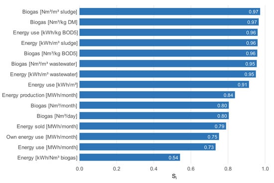
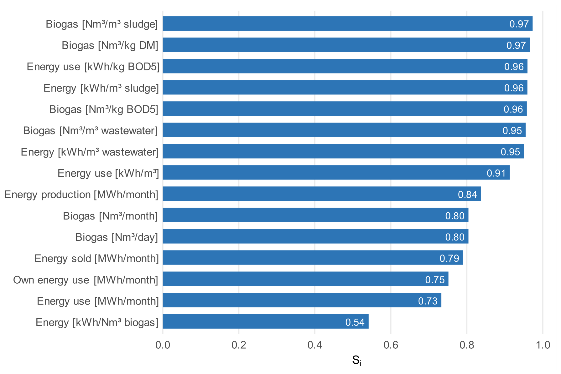
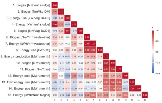
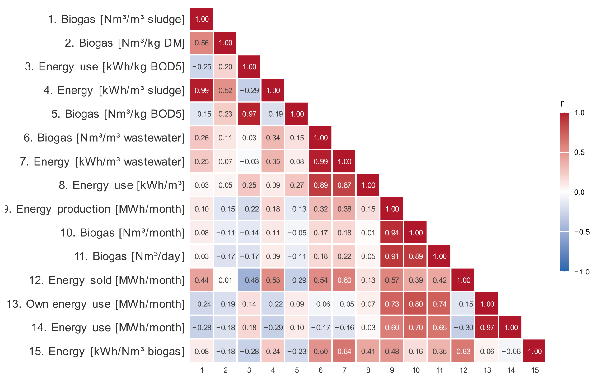
Using the principal components obtained, we assessed the feasibility of modeling the 15 previously identified energy indicators. For each indicator, the sum of the squares of the Pearson linear correlation coefficients with the principal components was calculated according to the formula
where Yi denotes the i-th energy indicator, PCj denotes the j-th retained principal component, and r(Yi,PCj) is the Pearson linear correlation coefficient between them. The calculations were performed exclusively on the training set so that the selection of response variables would be independent of the information contained in the test set. Due to the mutual orthogonality of the components, this measure determines what portion of a given indicator’s variability can potentially be reconstructed based on the retained components (Figure 4). For further modeling, three indicators were selected that exhibit high values of this measure and simultaneously represent different aspects of the wastewater treatment plant’s energy management: unit biogas production per unit of dry sludge mass [Nm3/kg DM], energy production from sludge [kWh/m3 sludge], and energy consumption per unit of removed biochemical oxygen demand (BOD5) [kWh/kg BOD5]. The Biogas [Nm3/kg DM] variable was selected instead of Biogas [Nm3/m3 sludge] (despite a similar correlation result with the predictors) because the Biogas [Nm3/m3 sludge] variable already had a high correlation with the Energy [kWh/m3 sludge] variable (Figure 5), making the set of output variables more representative.
Figure 4.
Values of the Si metric for the analyzed energy indicators.
Figure 5.
Correlation matrix of the analyzed energy indicators in the training set.
2.4. Predictive Models
The main predictive model was a multilayer perceptron (MLP), which was compared with three reference models: random forest, support vector regression with a linear kernel (SVR), and the XGBoost regression model. All models were built on the same input representation comprising 11 principal components and trained separately for each of the three selected response variables.
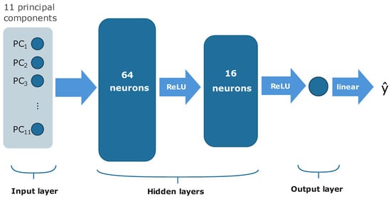
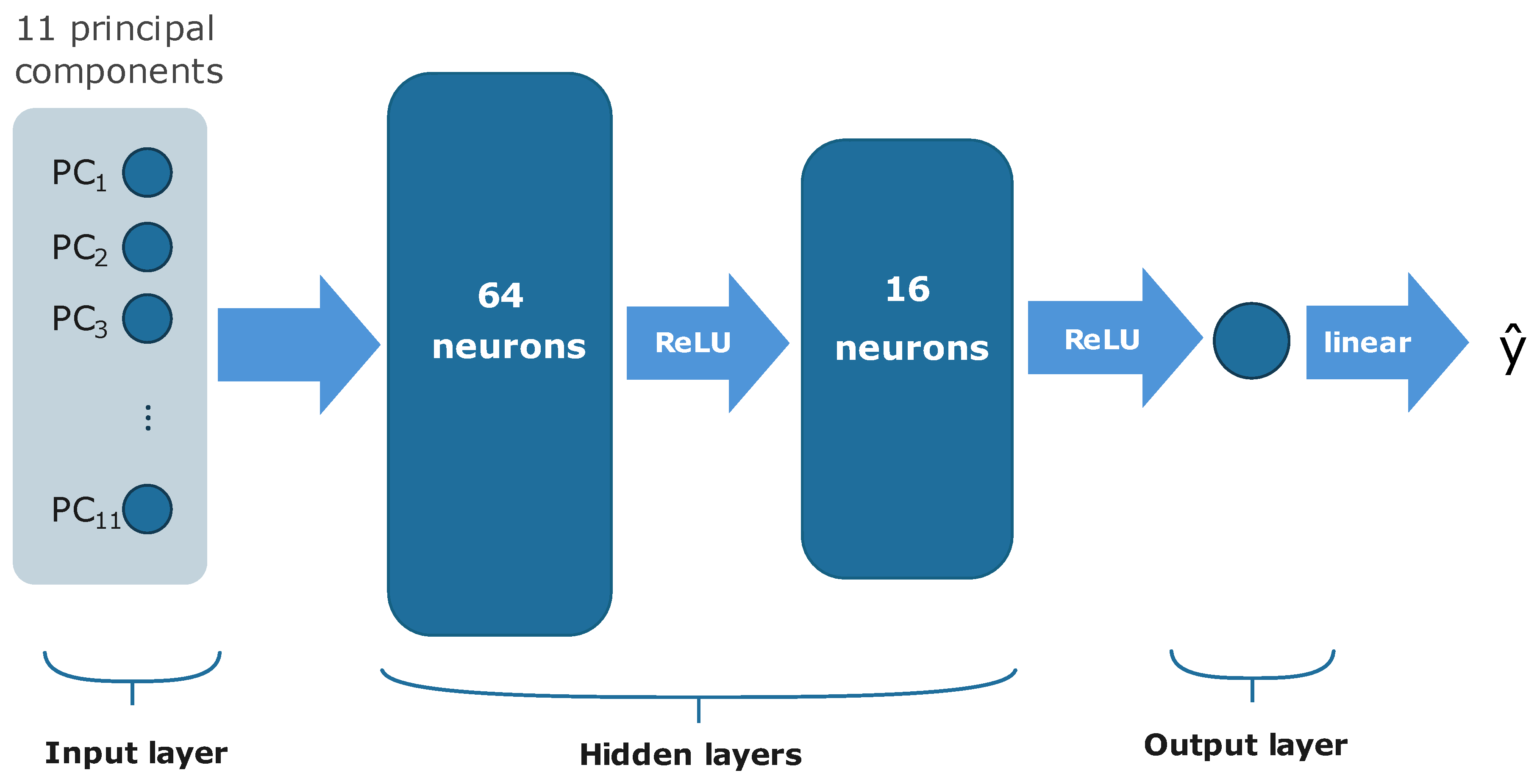
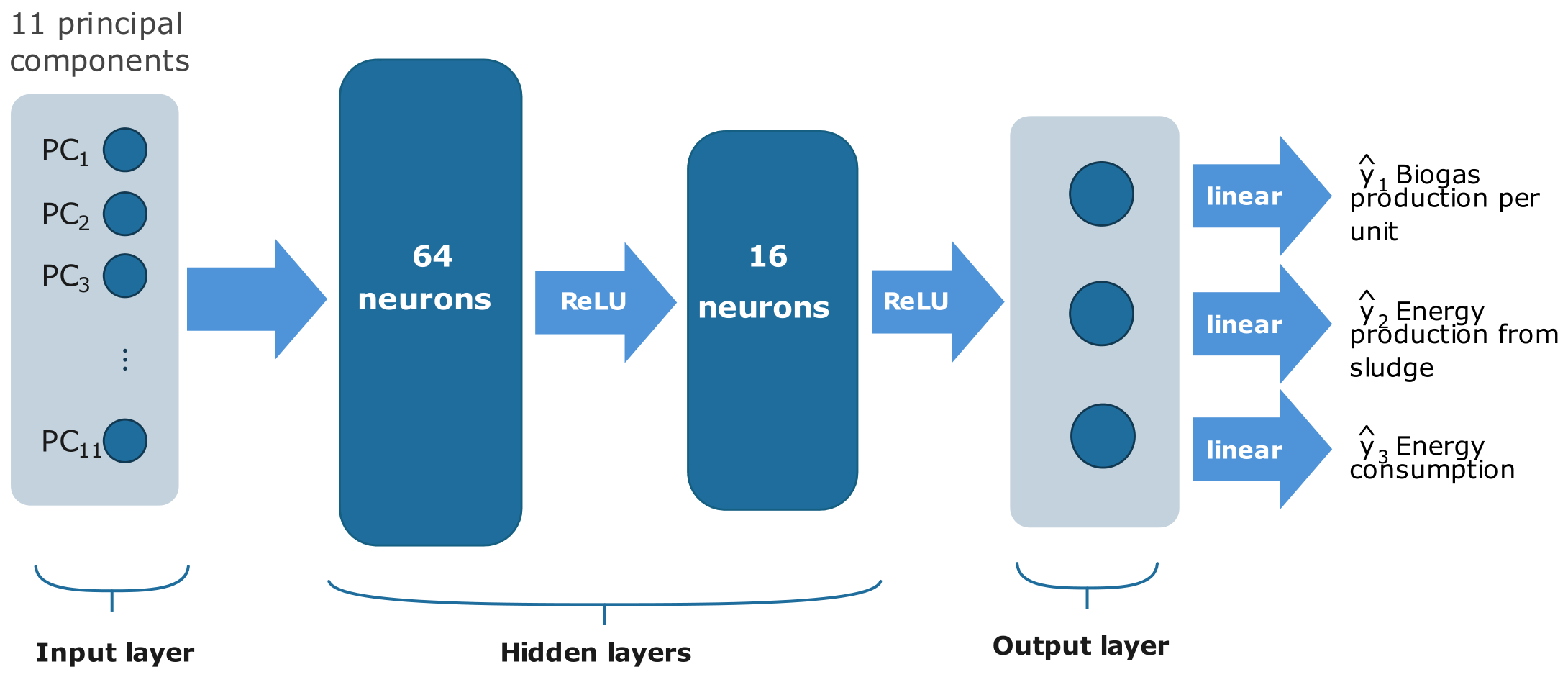
The same neural network architecture was used for all three modeled variables: an 11-element input vector corresponding to the retained principal components, two hidden layers containing 64 and 16 neurons, respectively, with the Rectified Linear Unit (ReLU) activation function, and a single-neuron output layer with a linear activation function (Figure 6). It is worth noting here that performing a PCA on the original, standardized data can be equated, in the full model, with the application of one additional linear layer, whose estimation is performed independently of the training of the neural network or any other predictive model. Before training the network, the principal components were subjected to additional standardization using the means and standard deviations determined from the training set. The dependent variable was subjected to analogous standardization, and the obtained predictions were then transformed back to their original scale.
Figure 6.
MLP scheme.
The networks were trained using the backpropagation method with the Nadam (Nesterov-accelerated Adaptive Moment Estimation) optimizer, minimizing the mean squared error (MSE).
2.5. Reference Models
Hyperparameter tuning for the reference models was performed using four-fold cross-validation on the first 28 observations. In each of the four runs, seven observations constituted the validation set, and the remaining 21 formed the training set, with the temporal order maintained within each fold. To prevent information leakage between the datasets, PCA was performed separately in each validation run, exclusively on its training set, while the validation observations were projected onto the resulting principal component space. For each hyperparameter configuration, RMSE and MAE were calculated based on the predictions obtained in all four validation runs. The configuration with the lowest RMSE value was considered the best, with MAE used as a secondary criterion. After selecting the best hyperparameter configuration, the model was retrained using all 28 observations from the training set, and its quality was then evaluated on seven observations from the test set. The hyperparameter search ranges used for the reference models are summarized in Table 1.
Table 1.
Hyperparameter search ranges for the reference models.
2.6. Model Quality Assessment
Prediction quality was assessed on a test set covering the last seven months. The following metrics were used: root mean square error (RMSE), mean absolute error (MAE), coefficient of determination R2, and the ratio of RMSE on the test set to RMSE on the training set. Their formulas are given below:
where yi denotes the actual value of the dependent variable for the i-th observation, represents the value predicted by the model, y is the mean value of the dependent variable, and n denotes the number of observations.
2.7. Selection of Model Configurations
As a result of tuning the reference models, different hyperparameter configurations were obtained for the individual indicators analyzed (Table 2). In the case of the MLP, the same 11-64-16-1 architecture, comprising 1825 parameters, was used for all indicators, while the settings and training processes of the individual models differed.
Table 2.
Hyperparameter values selected for individual models and energy metrics.
2.8. Software and Hardware
All analyses were performed in R 4.5.2. Neural network models were implemented using the R packages keras 2.16.1 and tensorflow 2.20.0 through reticulate 1.47.0, connected to Python 3.11.15 with TensorFlow 2.15.1, Keras 2.15.0, KerasTuner 1.4.6, NumPy 1.26.4, SciPy 1.17.1, and scikit-learn 1.9.0. Random seeds were fixed to improve reproducibility. A global seed of 123 was used in the R analyses and as the base seed for hyperparameter optimization. During neural network tuning and repeated model fitting, seeds were set jointly for Python, NumPy, and TensorFlow. Computational benchmarks were performed on a system equipped with an Intel Core i5-1240P processor (12 cores, 16 threads), using CPU-only TensorFlow execution with GPU acceleration disabled and intra- and inter-op parallelism limited to one thread. The entire process of tuning and retraining the best configurations took approximately 12 h for all MLP models combined. A single training run of the final MLP model (after tuning), for example, for energy production from sludge, took approx. 19.3 s, whilst a single prediction took approx. 62.9 ms.
3. Results
3.1. Prediction Quality on the Test Set
The MLP model achieved the best prediction quality for all three analyzed indicators (Table 3). Its advantage was particularly evident in the case of energy production from sludge and energy consumption. For unit biogas production, however, the results of the MLP and SVR models were similar, with R2 values of 0.906 and 0.874, respectively. The poorest prediction quality was observed for XGBoost.
Table 3.
Model results for the three energy metrics analyzed.
The results reveal clear differences in the predictability of the three analyzed indicators. Specific biogas production was predicted with the highest accuracy, whereas energy production from sludge showed considerably lower, although still useful, prediction performance. This indicates that the process variables used in the analysis contain more consistent information about the biological stage of anaerobic digestion than about the subsequent conversion of the generated biogas into useful energy.
The high predictive performance obtained for specific biogas production is consistent with the authors’ previous research on machine learning-based prediction of anaerobic digestion performance [11,16]. In earlier studies, machine learning models were used to relate sludge characteristics and operational parameters to biogas production, while the present study extends this approach by considering a broader set of technological and physicochemical variables.
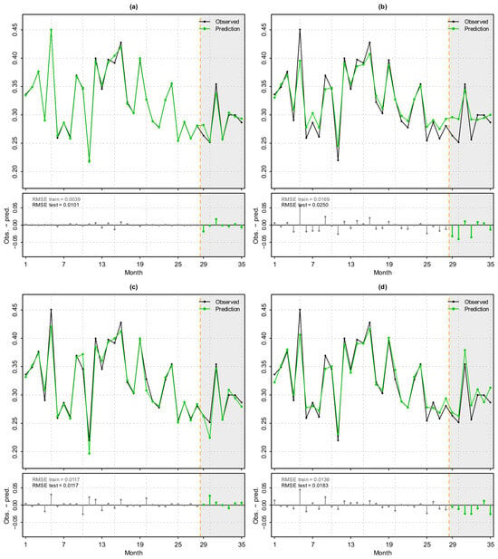
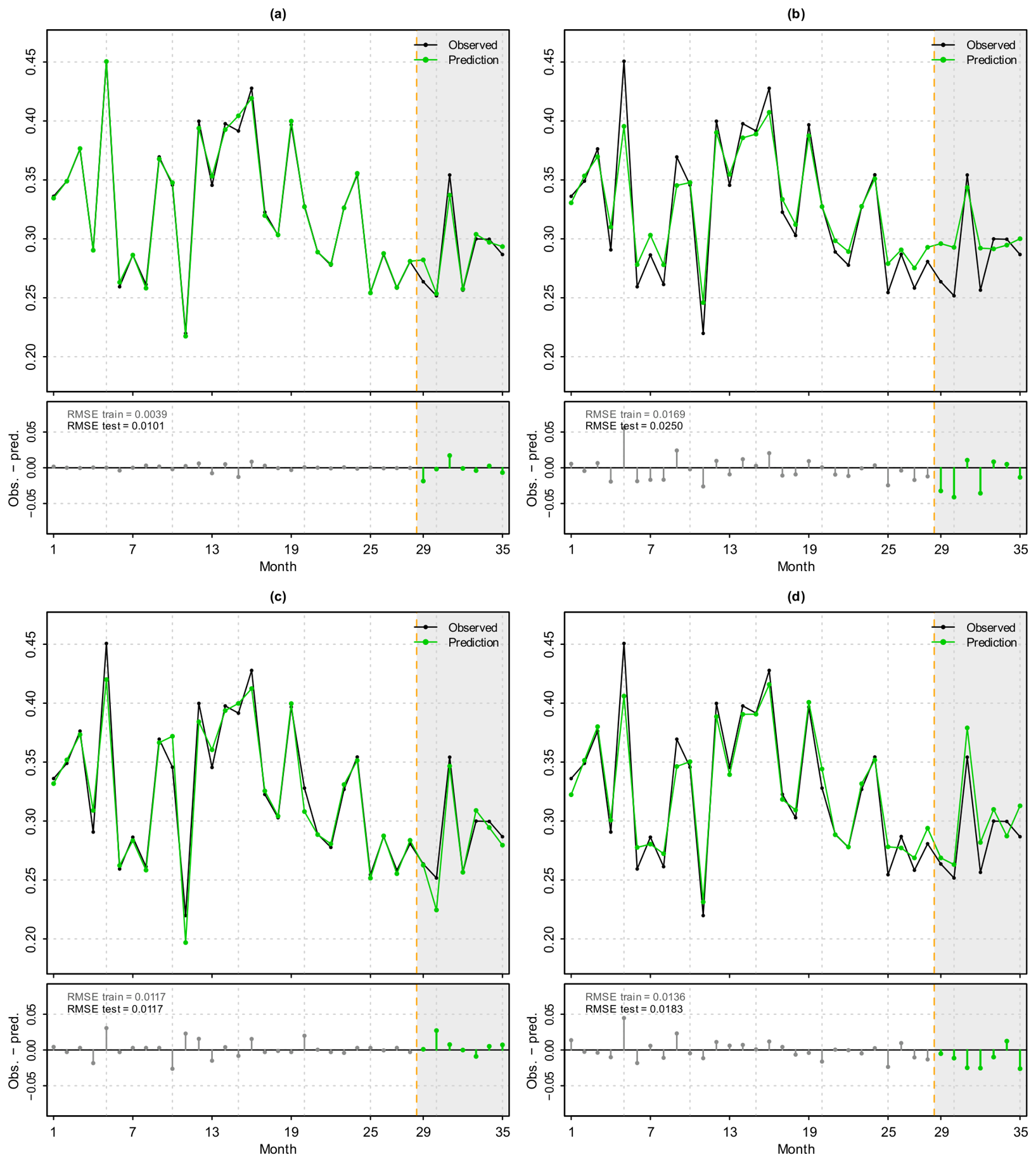
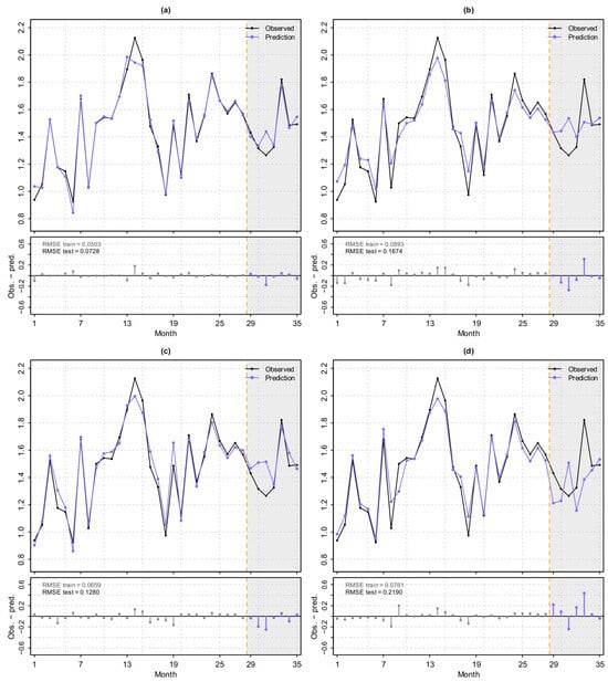
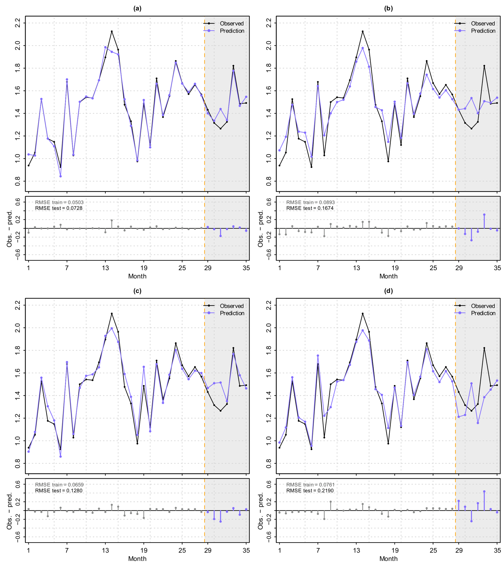
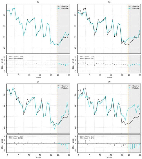
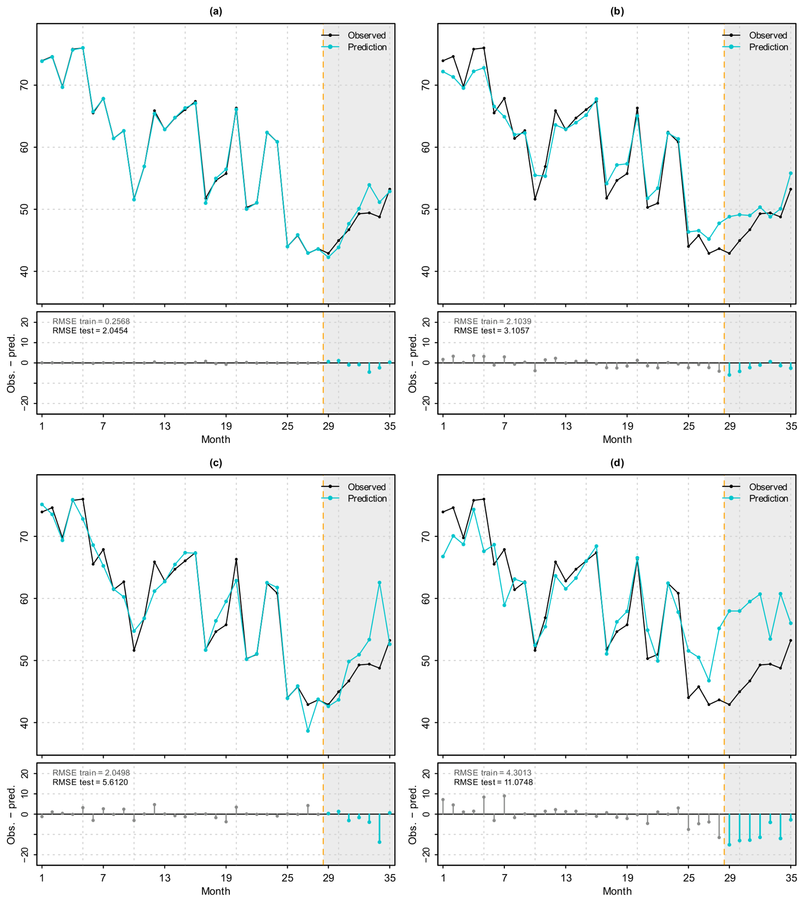
The trends in actual and predicted values over the following months are shown in Figure 7, Figure 8 and Figure 9. For each of the modeled variables, the MLP-based model achieved the best results on the test set. The results suggest that the easiest variable to model was Biogas production per unit [Nm3/kg DM]. In fact, all models performed worst when predicting energy production from sludge [kWh/m3 sludge], showing a clear tendency to overestimate the results for this particular energy variable.
Figure 7.
Observed and predicted values of specific biogas production for (a) MLP, (b) random forest, (c) SVR, and (d) XGBoost. In each panel, the upper plot shows the observed (black) and predicted values, and the lower plot shows the residuals (observed–predicted) over time, with training-period residuals in grey and test-period residuals in color. The orange dashed line marks the boundary between the training period (months 1–28) and the test period (months 29–35, shaded).
Figure 8.
Actual and predicted values of unit energy consumption: (a) MLP, (b) random forest, (c) SVR, and (d) XGBoost. In each panel, the upper plot shows the observed (black) and predicted values, and the lower plot shows the residuals (observed–predicted) over time, with training-period residuals in grey and test-period residuals in color. The orange dashed line marks the boundary between the training period (months 1–28) and the test period (months 29–35, shaded).
Figure 9.
Actual and predicted values of energy production from sludge: (a) MLP, (b) random forest, (c) SVR, and (d) XGBoost. In each panel, the upper plot shows the observed (black) and predicted values, and the lower plot shows the residuals (observed–predicted) over time, with training-period residuals in grey and test-period residuals in color. The orange dashed line marks the boundary between the training period (months 1–28) and the test period (months 29–35, shaded).
For biogas production, the MLP predictions followed the observed temporal pattern relatively closely, and the model was able to reproduce changes in the target variable during the test period. In contrast, the larger deviations observed for energy production from sludge indicate that this variable may be characterized by a more complex relationship with the available process information.
The results obtained at this stage already confirm the superiority of the MLP models; however, the high values of the RMSEratio suggest that the model architecture could still be improved, as the current model may be prone to overfitting. For this reason, the issue of tuning MLP models will be discussed later in this paper.
The RMSEratio provides complementary information to R2 because it allows the difference between training and test errors to be assessed. The particularly high value obtained for energy production from sludge indicates a substantial discrepancy between training and test performance. This observation provided the rationale for the subsequent hyperparameter optimization and the introduction of regularization.
3.2. Training Process for MLP Models
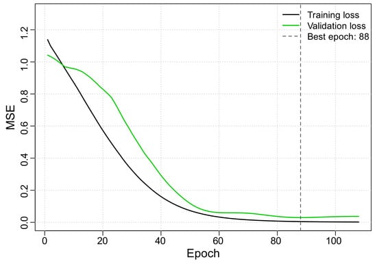
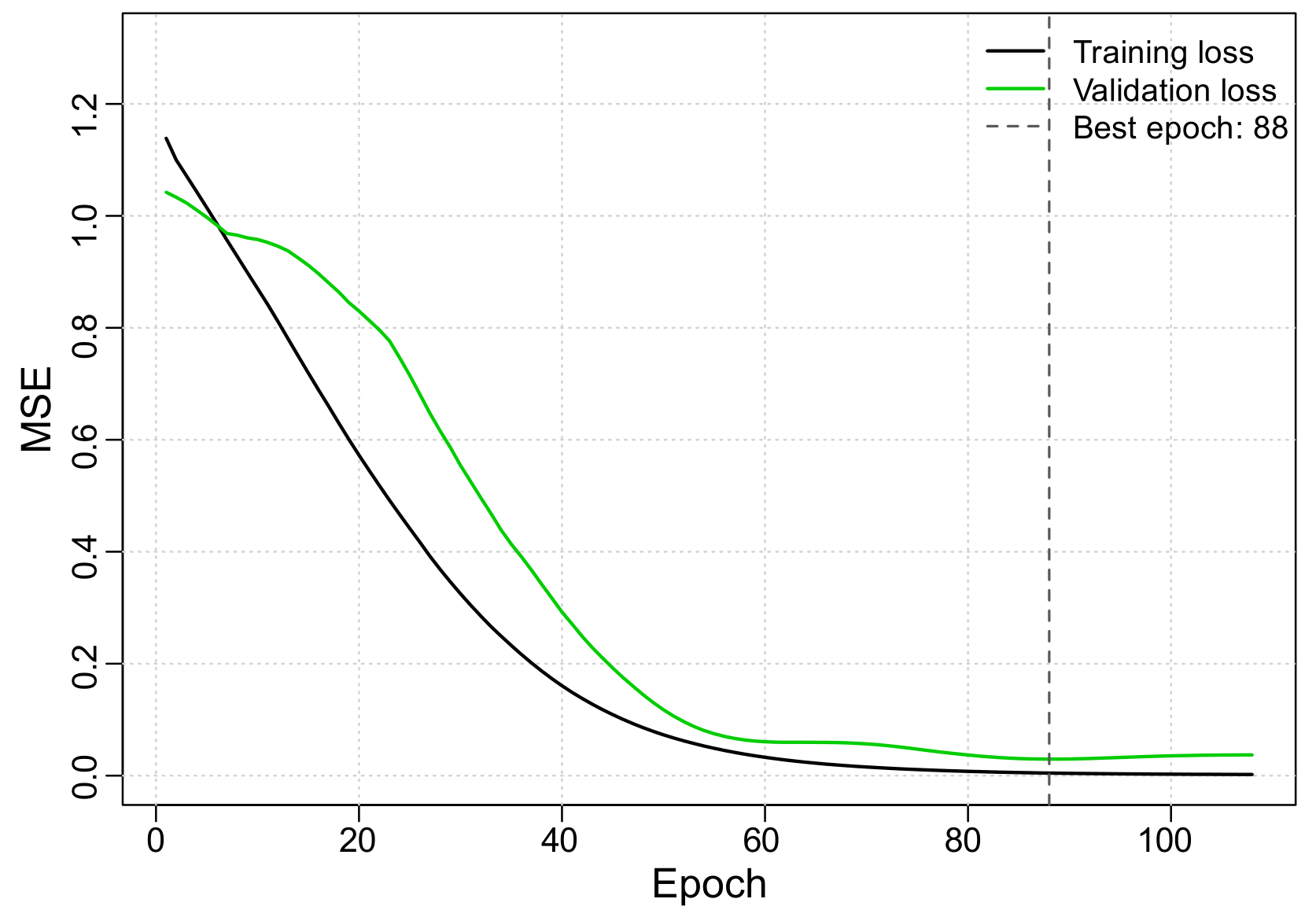
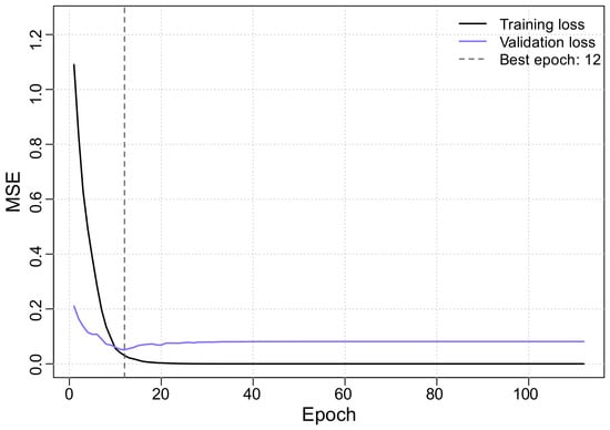
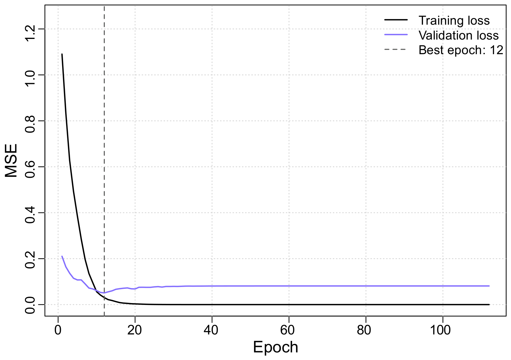
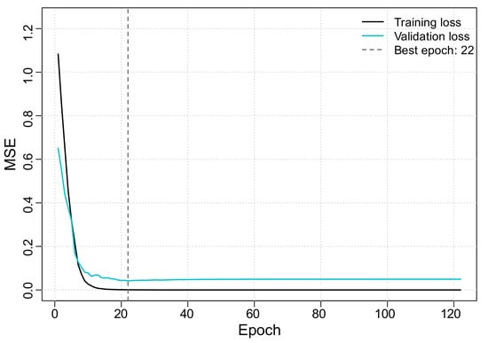
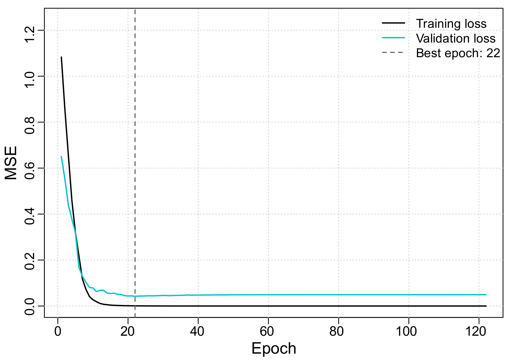
The point at which the validation loss function reached its minimum and the total number of training epochs varied among the three MLP models. For unit biogas production, the lowest value of the validation loss function was reached in the 88th epoch, and the training process ended after 108 epochs (Figure 10). In the case of energy production from sludge, the minimum was reached earlier, in the 22nd of 122 completed epochs (Figure 11). For unit energy consumption, the minimum of the validation loss function occurred in the 12th epoch, while training was completed after 112 epochs (Figure 12). The differences in the number of epochs ran resulted from the use of a callback that reduced the learning rate in the absence of improvement in the validation loss function, which allowed for adaptive adjustment of the learning process for each model.
Figure 10.
Loss function curve during the training of the MLP model for unit biogas production.
Figure 11.
Loss function curve during the training of the MLP model for unit energy consumption.
Figure 12.
Loss function curve during the training of the MLP model for energy production from sludge.
The different positions of the minimum validation loss indicate that the three prediction tasks had different learning dynamics. The relatively early minimum obtained for energy production from sludge and energy consumption suggests that further training of the baseline networks did not improve their validation performance. In contrast, the later minimum observed for specific biogas production indicates that more training iterations were required to capture the relationships between the process variables and the target indicator. This observation is consistent with previous work of the authors, in which differences in model performance were associated with the structure and variability of the available data, as well as with the selected modeling approach [11,16]. In particular, the earlier studies demonstrated that the characteristics of individual anaerobic digesters and the selection of the input variables may affect the generalization of machine learning models.
3.3. Supplementary Tuning of MLP Model Hyperparameters
To verify whether the prediction quality of multilayer neural networks could be improved by optimizing the architecture and training parameters, an additional tuning procedure was conducted. Although the prediction quality of the MLP models was better than that of the reference models, the elevated RMSEratio values—particularly for energy production from sludge—suggested the possibility of overfitting the models to the training data. For this reason, the tuning scope was expanded to include dropout and L2, regularization, which were intended to limit model overfitting.
The same input data representation as in the main analysis was retained. Tuning was performed for two variants of MLP models: three independent single-output models, trained separately for each indicator, and one multi-output model that predicts all three indicators simultaneously using shared hidden layers. In both variants, Bayesian optimization implemented in KerasTuner was used. The same range of hyperparameters was searched for both the single-output models and the multi-output model (Table 4), and all networks used the ReLU activation function in the hidden layers, the Nadam optimizer, and MSE as the loss function. During the optimization phase, each configuration was trained for a maximum of 300 epochs, with early stopping applied after 60 epochs if there was no improvement in the validation loss. In the retraining phase of the selected configurations, the maximum number of epochs was increased to 1000, and the early stopping criterion was set to 100 epochs without improvement. In both stages, adaptive learning rate reduction was applied in the absence of improvement in the validation loss function.
Table 4.
Hyperparameter search ranges.
For each of the three single-output models, Bayesian optimization was performed, involving the evaluation of 60 hyperparameter configurations on the validation set. Next, for each model, the 10 best unique hyperparameter configurations were selected, and each was trained 50 times with different weight initializations, resulting in a total of 500 additional runs for each dependent variable. From among these runs, the best model for a given indicator was selected. For each target, the final single-output model was selected as the run with the lowest validation RMSE among all 10 × 50 runs. A similar procedure was applied to the multi-output model, which predicted the three standardized target variables simultaneously using shared hidden layers and a three-neuron linear output layer. As in the single-output analysis, 60 hyperparameter configurations were evaluated, after which the 10 best unique configurations were selected and each was retrained 50 times with different weight initializations. Unlike the single-output models, which were selected separately for each target based on the validation RMSE, the multi-output model was optimized jointly for all three targets. The final multi-output model was selected as the run with the lowest joint validation loss (MSE) among all 10 × 50 retraining runs. Target-specific performance metrics were then calculated separately for each of the three output variables after transforming the predictions back to their original scales. The best single-output models differed in both architecture and regularization level (Table 5).
Table 5.
Best MLP model configurations obtained during tuning.
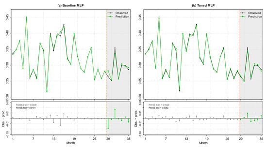
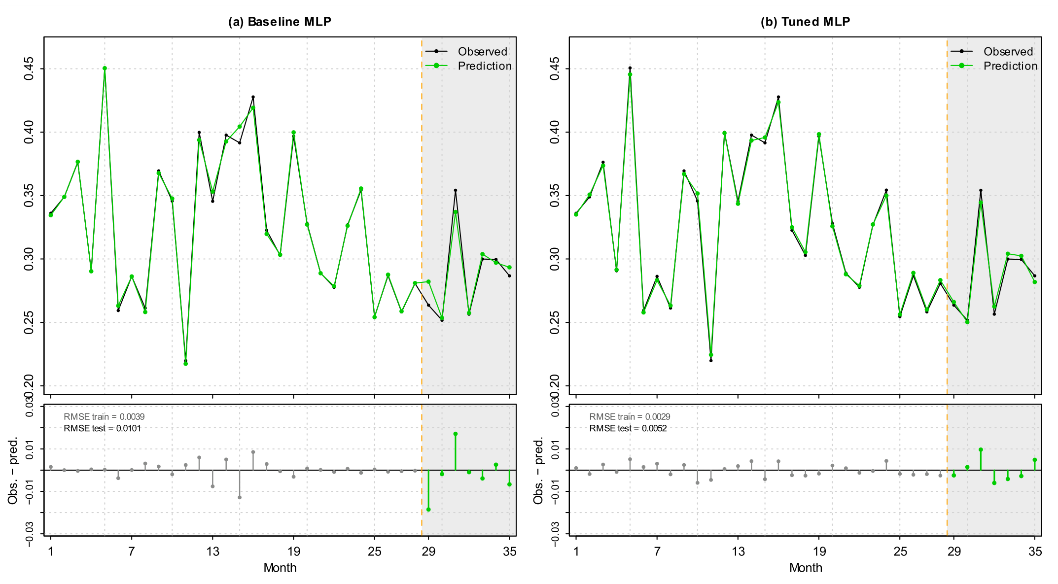
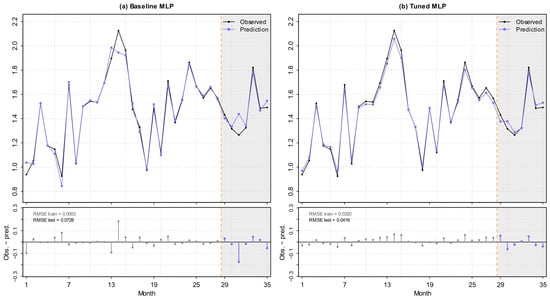
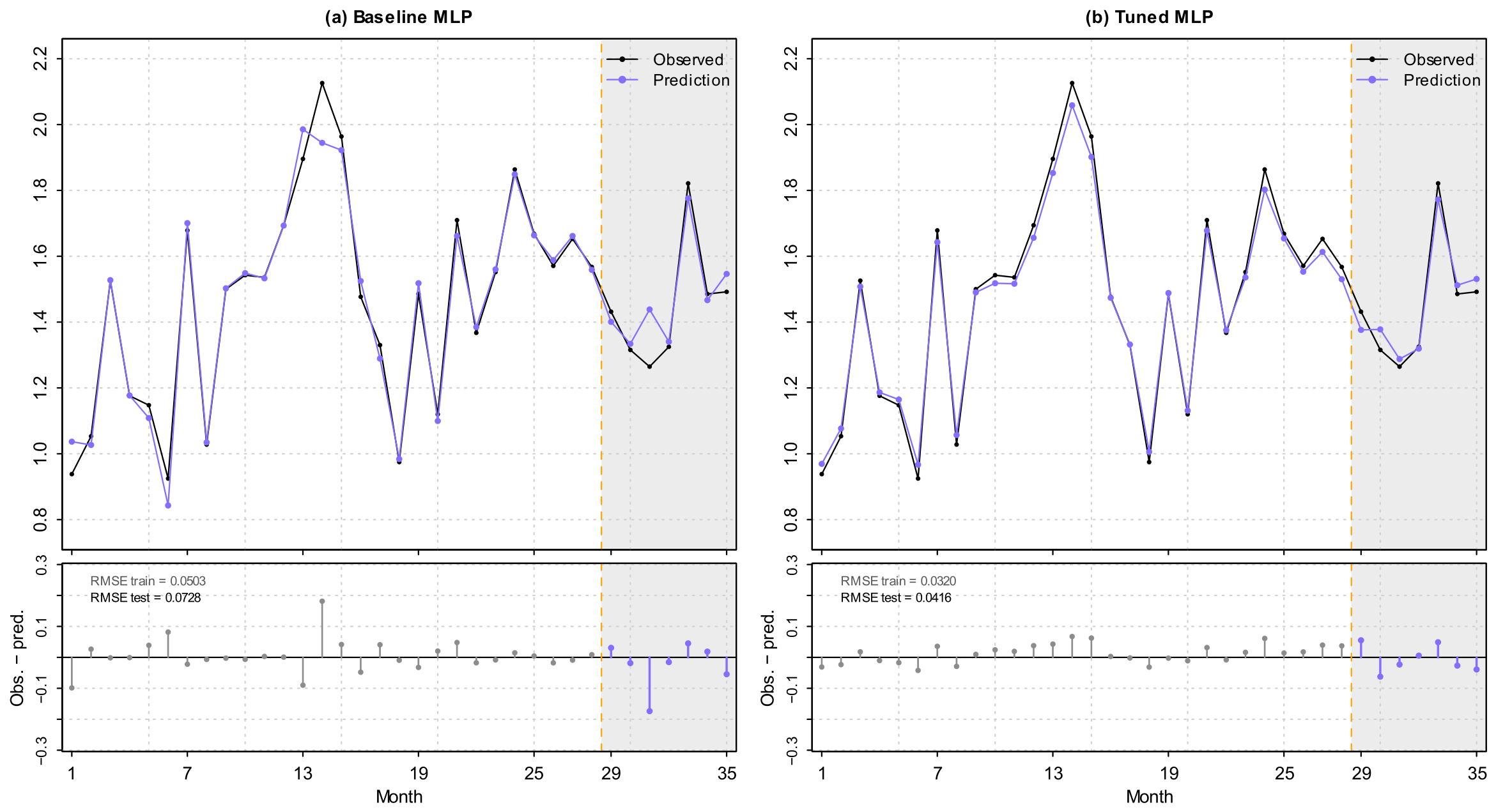
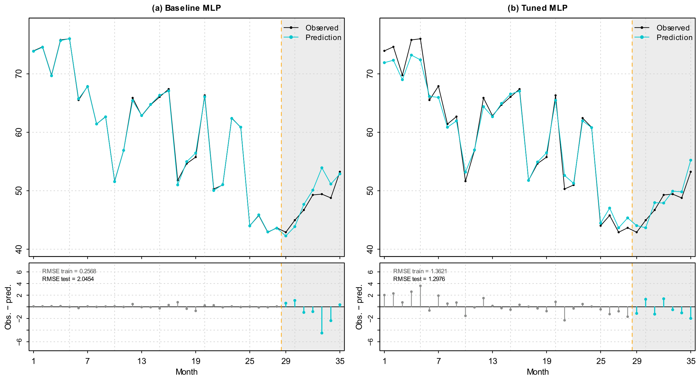
The best single-output models identified through the extended tuning procedure achieved lower RMSE values on the test set than the corresponding MLP models used in the baseline analysis. For unit biogas production, RMSE decreased from 0.0101 to 0.0052; for energy production from sludge, from 2.0454 to 1.2976; and for unit energy consumption, from 0.0728 to 0.0416 (Table 6). As a result of the tuning, the configurations with a low or moderate dropout rate and a low L2 penalty were selected, and the RMSEratio values decreased for all three indicators compared to the baseline analysis. This implies a smaller disparity between the error on the training and test sets, indicating a reduced risk of overfitting in the models.
Table 6.
Prediction quality of the best MLP models identified during the tuning procedure.
The importance of model optimization is consistent with the findings of Organiściak et al. [18], who compared several machine learning algorithms and ensemble configurations for biogas-yield prediction using 860 observations. Their results demonstrated that model performance depends not only on the selected algorithm but also on the structure and size of the dataset. The present results further indicate that, for neural network models, systematic hyperparameter optimization and regularization can substantially improve predictive accuracy.
A comparison of the trends in actual and predicted values for the baseline models and the models selected through the tuning procedure is presented in Figure 13, Figure 14 and Figure 15.
Figure 13.
Comparison of specific biogas production predictions for (a) the baseline and (b) the tuned MLP model. Upper plots: observed (black) and predicted values; lower plots: residuals (observed–predicted) for the training (grey) and test (color) periods, with RMSE given separately for each period. The orange dashed line marks the boundary between the training (months 1–28) and test (months 29–35, shaded) periods. The metrics in Table 6 refer exclusively to the test period.
Figure 14.
Comparison of unit energy consumption predictions for (a) the baseline and (b) the tuned MLP model. Upper plots: observed (black) and predicted values; lower plots: residuals (observed–predicted) for the training (grey) and test (color) periods, with RMSE given separately for each period. The orange dashed line marks the boundary between the training (months 1–28) and test (months 29–35, shaded) periods. The metrics in Table 6 refer exclusively to the test period.
Figure 15.
Comparison of predictions for energy production from sludge for (a) the baseline and (b) the tuned MLP model. Upper plots: observed (black) and predicted values; lower plots: residuals (observed–predicted) for the training (grey) and test (color) periods, with RMSE given separately for each period. The orange dashed line marks the boundary between the training (months 1–28) and test (months 29–35, shaded) periods. The metrics in Table 6 refer exclusively to the test period.
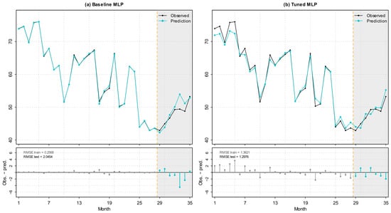
The graphical comparison confirms the numerical results presented in Table 6. The tuned models generally followed the observed trajectories more closely than the baseline models, particularly during the test period. The value of RMSEratio = 0.9526 can be considered slightly low, suggesting that the model performed better on the test data. However, from a statistical point of view, for the F-distribution we know that , so the obtained result is not particularly concerning.
3.4. Multi-Output MLP Model
The optimized multi-output MLP consisted of 11 input variables corresponding to the retained principal components, two shared hidden layers with 64 and 16 neurons, respectively, and a three-neuron linear output layer corresponding to the three predicted indicators. The model contained 1859 trainable parameters. The hidden layers were shared by all three prediction tasks, whereas each output neuron represented one of the target variables. The architecture of the optimized multi-output model is presented in Figure 16.
Figure 16.
Architecture of the optimized multi-output MLP model.
The optimized multi-output model used 64 and 16 neurons in its two hidden layers, corresponding to the maximum hidden-layer widths considered during hyperparameter tuning. Its hidden architecture was therefore wider than those selected for the single-output models for specific biogas production (64-4-1) and energy production from sludge (16-16-1), and had the same hidden-layer widths as the single-output model for energy consumption (64-16-1). The multi-output model contained 1859 trainable parameters, compared with 1033, 481, and 1825 parameters in the respective single-output models. Although the optimized multi-output model was not narrower than the single-output models in terms of hidden-layer widths, it achieved poorer predictive performance for all three target variables, with the greatest deterioration observed for energy production from sludge (Table 7).
Table 7.
A comparison of the best single-output and multi-output models.
For specific biogas production, R2 decreased from 0.9752 for the optimized single-output model to 0.7402 for the multi-output model, while RMSE increased from 0.0052 to 0.0168. An even greater deterioration occurred for energy production from sludge, for which R2 decreased from 0.8281 to −0.6443. For energy consumption, R2 decreased from 0.9420 to 0.7298. These results show that, for the investigated WWTP, the separately optimized single-output models achieved substantially better test-set performance than the shared multi-output model.
Thus, under the modeling procedure used in this study, simultaneous prediction using shared hidden layers did not provide an advantage over separately optimized single-output networks. One possible explanation is that, although the three indicators are related within the WWTP energy system, they characterize different aspects of plant operation and may differ in how strongly and in what way they are related to the available technological and physicochemical variables. Under such conditions, using a single shared hidden representation for all three prediction tasks does not necessarily improve predictive performance compared with optimizing each task separately. However, the poorer performance of the multi-output model should not be interpreted as evidence that the three target variables are statistically independent or that multi-output modeling is generally unsuitable for this type of problem. The present comparison was based on a relatively small dataset from a single WWTP and on the class of shared MLP architectures considered in this study. Further studies using larger datasets and alternative multi-task architectures would be required to determine whether the observed advantage of separately optimized models is generalizable.
This finding is consistent with the broader development of the authors’ machine learning research. The earlier AD2Biogas study demonstrated the practical usefulness of a model dedicated to biogas prediction [11], while the subsequent meta-regression study investigated the combination of predictions from different models [16]. More recently, the authors extended the approach toward predictive control by combining random forest with a Genetic Algorithm and incorporating meteorological conditions as external disturbances [15]. The present results indicate that, when several energy indicators are considered simultaneously, a target-specific modeling strategy may be preferable to a single shared architecture.
4. Conclusions and Future Research Directions
The experiments conducted demonstrated that a multilayer neural network allows for highly accurate modeling of selected energy factors related to the operation of a wastewater treatment plant. The use of model optimization techniques—cross-validation (base models) and hyperparameter tuning (neural network)—strengthens the argument that a multilayer neural network has the greatest potential for accurate and reliable prediction.
It is worth noting that despite the use of a multilayer network architecture, the use of PCA-based reduction allows us in this case to consider a wide range of 41 physical parameters and end up with final neural models that have a relatively small number of parameters—on the order of a few thousand weights. This model size allows for the widespread application of this type of analysis: training and optimizing the models—including for other potential facilities—requires only a mid-range PC, and the target model size allows for its integration at the inference level within existing IT systems.
The results obtained suggest conducting a broader analysis covering subsequent years of the treatment plant’s operation, and the use of a multilayer neural network with ReLU activations offers another significant opportunity—since the finished, trained model is described by an explicit, differentiable function, and owing to the model’s good fit to the actual data, it is possible to reliably calculate the local gradient of the output variables with respect to the input parameters—which, in turn, provides a basis for investigating changes in the treatment plant’s operation that would contribute to optimizing energy production. Quantifying this using a well-chosen neural network therefore also allows for a precise analysis of the benefits and costs of such optimization—this task will be the main focus of the authors’ future work.
This direction is consistent with the authors’ previous research, which has progressively developed from machine learning-based prediction of biogas production [11,18] toward the use of optimization algorithms and external variables for predictive control of anaerobic digestion [15]. The present study therefore provides a further step toward an integrated prediction–optimization framework for improving the energy efficiency and self-sufficiency of wastewater treatment plants. At the same time, the high predictive performance obtained in this study should be interpreted in relation to the specific WWTP and dataset analyzed. The models were developed using data from a single facility; therefore, their transferability to other wastewater treatment plants, technologies and operating conditions requires further validation.
Another interesting aspect of this study is that, because the data come from real-world measurements, the final model has relatively few parameters; thus, both the problem and the resulting model are ideally suited for conducting preliminary research on new methods of training neural networks—ones that are not based on gradient descent. The models obtained in this paper can serve as an ideal benchmark for this type of numerical experiment.
Author Contributions
Conceptualization, A.M., K.K. and G.Ł.; methodology, K.K. and G.Ł.; software, K.K. and A.G.; validation, A.M., K.K. and G.Ł.; formal analysis, A.M., K.K., J.C., A.S. and G.Ł.; investigation, All authors; resources, A.M., K.K., A.G. and J.C.; data curation, A.M. and K.K.; writing—original draft preparation, K.K., A.G. and A.S.; writing—review and editing, A.M., J.C., A.S. and G.Ł.; visualization, K.K. and A.G.; supervision, A.M., K.K. and G.Ł.; project administration, K.K. and G.Ł.; funding acquisition, K.K. and G.Ł. All authors have read and agreed to the published version of the manuscript.
Funding
This work was financially supported within the authors’ research of particular scientific units under subvention for a Scientific Disciplines program (grant number of the Rzeszow University of Technology: PB29.BT.26.001.01; grant numbers of the Lublin University of Technology: FD-20/IS-6/021, FD-20/IS-6/036, FD-20/NZ-7/017; FD-20/NZ-7/071).
Data Availability Statement
Dataset available on request from the authors.
Acknowledgments
We gratefully acknowledge the Iława WWTP staff for their kind help.
Conflicts of Interest
The authors declare no conflicts of interest.
Abbreviations
The following abbreviations are used in this manuscript:
| AD | Anaerobic digestion |
| ADM1 | Anaerobic Digestion Model No. 1 |
| BOD5 | Biochemical Oxygen Demand |
| CHP | Combined Heat and Power units |
| COD | Chemical Oxygen Demand |
| DM | Dry matter |
| ES | Excess sludge |
| MAE | Mean absolute error |
| MLP | Multilayer perceptron |
| MSE | Mean squared error |
| Nadam | Nesterov-accelerated Adaptive Moment Estimation |
| PCA | Principal component analysis |
| PE | Population equivalent |
| PS | Primary sludge |
| ReLU | Rectified Linear Unit |
| RMSE | Root mean square error |
| SVR | Vector regression |
| TN | Total nitrogen |
| TP | Total phosphorus |
| TSS | Total Suspended Solids |
| WWTPs | Wastewater treatment plants |
Appendix A
Table A1.
Factor loadings of the process variables for the eleven principal components retained for modeling. Loadings with absolute values below 0.20 were omitted.
References
- Hamawand, I. Energy Consumption in Water/Wastewater Treatment Industry—Optimisation Potentials. Energies 2023, 16, 2433. [Google Scholar] [CrossRef] [Scilit]
- Csedő, Z.; Sinóros-Szabó, B.; Zavarkó, M. Seasonal Energy Storage Potential Assessment of WWTPs with Power-to-Methane Technology. Energies 2020, 13, 4973. [Google Scholar] [CrossRef] [Scilit]
- Taiwo, K.J.; Oancea, A.V.; Kotha, N.S.; Usack, J.G. Enhancing Wastewater Treatment Sustainability Through Integrated Anaerobic Digestion and Hydrothermal Carbonization: A Life-Cycle Perspective. Sustainability 2025, 17, 7545. [Google Scholar] [CrossRef] [Scilit]
- Huang, M.-M.; Pan, M.-H.; Chang, F.-Y.; Chen, C.-C.; Lin, C.-Y. Reduction of Energy Consumption and Greenhouse Gas Emissions in Wastewater Treatment Plant: A Case Study of Utilizing Anaerobic Sludge Digestion. Next Energy 2025, 7, 100289. [Google Scholar] [CrossRef] [Scilit]
- Rossano-Becerril, S.; Sleutels, T.; Euverink, G.-J.W. Enhancing Sludge Management Efficiency through Thermal Hydrolysis: A System-Wide Analysis from Biogas Production to Dewatering. Biomass Bioenergy 2026, 208, 108865. [Google Scholar] [CrossRef] [Scilit]
- Andrade Cruz, I.; Silva Nascimento, V.R.; Alves Felisardo, R.J.; Gualberto Dos Santos, A.M.; Alles De Jesus, A.; Rego De Vasconcelos, B.; Kumar, V.; Bezerra Cavalcanti, E.; Lucena De Souza, R.; Romanholo Ferreira, L.F. Evaluation of Artificial Neural Network Models for Predictive Monitoring of Biogas Production from Cassava Wastewater: A Training Algorithms Approach. Biomass Bioenergy 2023, 175, 106869. [Google Scholar] [CrossRef] [Scilit]
- Samkhaniani, M.; Moghaddam, S.S.; Mesghali, H.; Ghajari, A.; Gozalpour, N. A Machine Learning Approach to Feature Selection and Uncertainty Analysis for Biogas Production in Wastewater Treatment Plants. Waste Manag. 2025, 197, 14–24. [Google Scholar] [CrossRef] [Scilit] [PubMed]
- Song, Q.; Hua, Y.; Yu, Y.; Chen, C.; Wu, B.; Dai, X. Impediments to Bioaccessibility in the Anaerobic Digestion of Waste Activated Sludge: An in-Depth Review of Challenges and Influencing Factors. Energy Environ. Sustain. 2025, 1, 100026. [Google Scholar] [CrossRef] [Scilit]
- Wang, Y.; Huntington, T.; Scown, C.D. Tree-Based Automated Machine Learning to Predict Biogas Production for Anaerobic Co-Digestion of Organic Waste. ACS Sustain. Chem. Eng. 2021, 9, 12990–13000. [Google Scholar] [CrossRef] [Scilit]
- Asadi, M.; Guo, H.; McPhedran, K. Biogas Production Estimation Using Data-Driven Approaches for Cold Region Municipal Wastewater Anaerobic Digestion. J. Environ. Manag. 2020, 253, 109708. [Google Scholar] [CrossRef] [Scilit] [PubMed]
- Organiściak, P.; Masłoń, A.A.; Kowal, B.; Kuraś, P.; Wadiak, B.; Sikorska-Czupryna, S.; Vanivska, V. Machine Learning-Based Prediction of Biogas Production from Sludge Characteristics in Four Anaerobic Digesters: Development of the AD2Biogas Prediction Tool. Adv. Sci. Technol. Res. J. 2024, 18, 1–15. [Google Scholar] [CrossRef] [Scilit] [PubMed]
- Ling, J.Y.X.; Chan, Y.J.; Chen, J.W.; Chong, D.J.S.; Tan, A.L.L.; Arumugasamy, S.K.; Lau, P.L. Machine Learning Methods for the Modelling and Optimisation of Biogas Production from Anaerobic Digestion: A Review. Environ. Sci. Pollut. Res. 2024, 31, 19085–19104. [Google Scholar] [CrossRef] [Scilit] [PubMed]
- Sadoune, H.; Rihani, R.; Marra, F.S. DNN Model Development of Biogas Production from an Anaerobic Wastewater Treatment Plant Using Bayesian Hyperparameter Optimization. Chem. Eng. J. 2023, 471, 144671. [Google Scholar] [CrossRef] [Scilit]
- Lucas, D.; Oliveira, P.; Bessa, A.; Marcondes, F.S.; Rodrigues, M. Towards Efficient Biogas Production: Deep Learning-Based Methane Forecasting in Anaerobic Digesters of Wastewater Treatment Plants. In Highlights in Practical Applications of Agents, Multi-Agent Systems and Computational Social Science. The PAAMS Collection; Communications in Computer and Information Science; Nongaillard, A., Caron, A.-C., González-Briones, A., Fernández, A., Durães, D., Sharaf, N., Eds.; Springer Nature: Cham, Switzerland, 2025; Volume 2644, pp. 154–165. ISBN 978-3-032-05924-6. [Google Scholar] [CrossRef] [Scilit]
- Organiściak, P.; Stęchły, A.; Kuraś, P.; Masłoń, A.; Turek, A. Machine-learning-based predictive control of anaerobic digestion considering meteorological conditions. Advs. Sci. Technol. Res. J. 2026, 20, 352–362. [Google Scholar] [CrossRef] [Scilit] [PubMed]
- Biogas Production Calculator (Rzeszów University of Technology). Available online: https://ad2biogas.tools.prz.edu.pl/ (accessed on 14 September 2026).
- Digester Biogas Yield Optimization (Rzeszów University of Technology). Available online: https://biogas-ga.streamlit.app/ (accessed on 14 September 2026).
- Organiściak, P.; Turek, A.; Stęchły, A.; Rysz, J.; Vanivska, V.; Masłoń, A.; Wadiak, B. Prediction of biogas yield from anaerobic digesters using meta-regression. Zesz. Nauk. SGSP/Szk. Gł. Służby Pożarniczej 2025, 93, 81–100. [Google Scholar] [CrossRef] [Scilit]

Disclaimer/Publisher’s Note: The statements, opinions and data contained in all publications are solely those of the individual author(s) and contributor(s) and not of MDPI and/or the editor(s). MDPI and/or the editor(s) disclaim responsibility for any injury to people or property resulting from any ideas, methods, instructions or products referred to in the content. |
© 2026 by the authors. Licensee MDPI, Basel, Switzerland. This article is an open access article distributed under the terms and conditions of the Creative Commons Attribution (CC BY) license.