


Abstract
Public buildings across Iraq draw their daytime electricity from small diesel generators running at low load. A photovoltaic battery supply for a girls’ primary school in Ramadi is assessed by hourly simulation against its 20 kVA diesel set, as a stand-alone system and as a hybrid that keeps the set as back-up. Demand was reconstructed from an appliance audit and the teaching calendar; generation was simulated from nineteen years of hourly satellite irradiance, and fuel use was taken from manufacturer data for a set of the same rating. A 19.44 kWp array with 28.7 kWh of lithium iron phosphate storage serves 95.0% of the 15,049 kWh annual demand on its own in the reference year, and between 92.6% and 98.1% across 2005–2023. With the set as backup, the whole demand is served, the set runs 232 h a year, and fuel use falls by 89%. The levelised cost of electricity is 0.120 USD kWh−1 for the hybrid and 0.093 USD kWh−1 for the stand-alone system, against 0.167 USD kWh−1 for diesel at the administered price of 0.19 USD L−1. The stand-alone system remains cheaper per kilowatt-hour even with free fuel; the hybrid is cheaper above 0.054 USD L−1. Greenhouse gas intensity falls from 1213 to 148 g CO2-eq kWh−1 with the hybrid, avoiding 10.4 t CO2-eq a year. On total cost, the hybrid breaks even with the existing supply at 0.21 USD L−1 and returns 23,572 USD over 25 years at product parity, so the case is marginal for the school at the pump price and strong for the state at the opportunity cost of its diesel.
1. Introduction
Electricity supply in Iraq has not kept pace with demand since the early 1990s, and interruptions of the public network reach eighteen hours a day in parts of the country [1]. Chronic under-investment, tariff subsidy, and transmission loss are all implicated, and the sector remains among the largest single calls on public capital expenditure [2,3,4]. The gap is filled by an estimated 55,000 to 80,000 privately operated diesel generators rated between 100 and 500 kVA, which supply neighbourhoods through isolated single-conductor distribution networks [1,5]. A much larger population of small sets is owned by individual buildings. Public-sector buildings sit in the second of those categories. A school, a clinic, or municipal office runs its own set for the working day, buys fuel from a budget line that is rarely audited against output, and receives no metered account of what the electricity costs. Sets of this kind run well below their rating for most of their hours. Measured specific fuel consumption in under-loaded diesel microgrids can exceed published values by a factor of five [6], and captive generators of the same class are a substantial urban source of air pollutants [7].
The solar resource that these buildings sit under is among the best in the world. Long-term horizontal irradiation across central and western Iraq lies between 4.6 and 5.2 kWh m−2 per day. National assessments place annual global irradiation between 2000 and 2500 kWh m−2 and attribute the slow uptake of solar supply to policy and institutional barriers rather than to the resource [8,9]. Reported specific yields for installed systems range from 1514 to 1745 kWh kWp−1 per year [10]. Module prices have fallen far enough that the capital barrier is no longer the module itself but the appropriation that buys it. What has changed more slowly is the evidence base a ministry would need in order to authorise replacement. Two questions decide the case: what the change costs, and what it saves in emissions. They are usually answered in separate papers, on separate system boundaries, for separate systems.
The environmental side of the question is well characterised at the technology level. Harmonisation of the published life-cycle assessments places crystalline-silicon photovoltaics at a median of 45 g CO2-eq kWh−1 under 1700 kWh m−2 per year of in-plane irradiation, an order of magnitude below fossil generation [11,12]. The most recent IEA PVPS Task 12 inventory update gives 35.8 g CO2-eq kWh−1 for a 3 kWp rooftop mono-crystalline system at 1331 kWh m−2 per year, with a non-renewable energy payback time of one year [13]. Values of that kind describe the module and the balance of system. They do not describe a stand-alone installation, which carries a battery. The battery is a substantial share of the burden: cradle-to-grave assessments of utility-scale photovoltaics with lithium-ion storage attribute 54% of total emissions to battery manufacture [14]. Divergence between published assessments is itself an active methodological question, and the harmonisation and parameterisation work of the past five years has narrowed it substantially [15,16].
Cell-level data for lithium iron phosphate have converged. A cost-based reconstruction of the global supply chain gives 54, 62, and 69 kg CO2-eq kWh−1 at the 5th, 50th, and 95th percentiles [17]. A process-based model for Chinese production gives 82.5 kg CO2-eq kWh−1 [18]. A parametric study spanning raw-material and grid conditions gives 90 to 127 kg CO2-eq kWh−1 for Chinese manufacture and 27 to 64 kg CO2-eq kWh−1 for Norwegian [19]. The spread is wide, but it is bounded, and it is small enough that a stand-alone system’s footprint can be stated with a defensible uncertainty range rather than omitted.
The economic side has been examined repeatedly for off-grid and hybrid supplies in weak-grid regions. An optimised hybrid mini-grid for Iraqi rural electrification reaches 0.123 USD kWh−1 [20]. Photovoltaic–diesel battery configurations for Iraqi villages and households are found economical against diesel-only supply in every configuration tested [21,22,23]. A Baghdad household study finds 0.077 USD kWh−1 for a grid-connected photovoltaic battery system against 0.126 USD kWh−1 for the grid-plus-generator arrangement it replaces [24]. Institutional cases outside Iraq run in the same direction. Reported figures are 0.125 USD kWh−1 for a remote school in Bangladesh [25] and 0.254 USD kWh−1 for a rural school in southern Ethiopia [26], with payback periods near five to six years for university buildings in Kenya and Mexico [27,28,29]. Closer to the present case in climate, air conditioning accounts for 80% of electricity end use in Saudi governmental schools, for which rooftop photovoltaics are assessed as a route to zero-energy operation [30]. At an educational building in Aswan, photovoltaic supply reduces grid use by 38% and emissions by 50% [31]. Diesel-only supply is consistently the worst option on cost in these comparisons, at 0.598 to 0.672 USD kWh−1 [10,32].
Three features of the institutional off-grid problem are under-treated in the studies cited above. The first is the seasonal relationship between a school’s demand and the solar resource. In a hot-arid climate, the two are in direct opposition for two months of the year: the array reaches its annual peak in July and August, when the building is empty. Sizing against a design day conceals this, and the penalty appears only as an unexplained gap between the specific yield and the energy actually used. Reliability-based sizing that simulates the loss of power supply hour by hour is well established [33,34], but it is commonly evaluated on one representative year and for loads that recur every day, not for a load that disappears for two months. The second is the price at which diesel is valued. Iraqi diesel sells at an administered pump price of roughly 0.19 USD L−1, a small fraction of international product parity. An analysis that assumes a market price will overstate the private saving by a factor of three or more; one that assumes the administered price will understate the saving to the state. The third is the absence of the photovoltaic system’s own life-cycle burden from studies that describe themselves as environmental assessments; where avoided emissions are computed as displaced diesel alone, the result is a gross figure, not a net one. Life-cycle comparisons of off-grid mini-grids in West Africa place fully photovoltaic supply with batteries at 0.10 to 0.16 kg CO2-eq kWh−1 and diesel at 1.14 kg CO2-eq kWh−1 [35]. Those figures indicate the size of the correction when storage and balance of system are counted.
The aim of this paper is to determine whether a photovoltaic battery supply, operated alone or with the existing generating set as back-up, would cost less and emit less over its life than the diesel supply of a diesel-dependent school, and under which fuel prices, reliability targets, and demand conditions that result holds. The case is an existing girls’ primary school in Ramadi supplied by a 20 kVA diesel set, for which the photovoltaic system is proposed rather than installed, so that its performance is simulated rather than measured. The novelty lies in treating the three points above together, on one hourly model and one system boundary, for a load that follows a school calendar, and in testing the reliability result against nineteen years of hourly satellite data rather than one synthetic year. The contributions are as follows.
- •
- An hourly demand model built from an appliance audit and the Iraqi teaching calendar, distinguishing cooling, heating, mild, and closed days, so that the seasonal mismatch is resolved rather than averaged away.
- •
- A storage design obtained by simulation over nineteen years of hourly satellite irradiance, with the power limits of the battery and charge controllers enforced, reported as energy- and time-based reliability indicators, together with a test of the common practice of synthesising hourly irradiance from monthly means.
- •
- A comparison of stand-alone and hybrid operation that quantifies the fuel, cost, and reliability exchanged when the existing generating set is kept as back-up.
- •
- A net greenhouse gas balance that carries the array, the balance of system, and the battery on the photovoltaic side and the fuel supply chain and genset manufacture on the diesel side, with a greenhouse gas payback time.
- •
- A life-cycle cost comparison expressed as break-even diesel prices on a levelised and a total-cost basis, with technical and economic parameters propagated by Monte-Carlo simulation, which separates the financial question facing the school from the economic question facing the state.
2. Materials and Methods
Four models are coupled over a common 25-year study period. Demand and photovoltaic generation are resolved hour by hour, and the system is simulated both stand-alone and with the existing generating set as back-up. Costs are discounted by the present-worth method of ASTM E917 [36], and greenhouse gases follow the IPCC 2006 inventory guidelines [37] with IPCC AR6 global warming potentials [38]. Performance indices follow the definitions of IEC 61724-1 [39]. All costs are expressed in constant 2026 United States dollars. The complete model is implemented as a single script so that every figure in Section 3 derives from one run; the loss chain, the dispatch rule, and the cost and emission factors are given in full below.
2.1. System Configuration
Three supply arrangements are available to an institutional building in Iraq and are shown schematically in Figure 1. A grid-connected system exports surplus generation and imports the shortfall, carries no storage, and therefore reaches the lowest levelised cost, but anti-islanding protection disconnects it during a network outage, which is precisely when the school needs it. A hybrid system keeps a diesel generator on the AC bus beside the array and a battery, so the generator covers any shortfall. It is the most reliable of the three, but it retains part of the fuel purchase and of the combustion emissions. A stand-alone system needs neither the network nor fuel and carries the array, charge control, battery, and inverter alone. The grid-connected arrangement is excluded because the public supply at the site is unavailable for most of the occupied day, so the export credit that justifies it does not exist. The stand-alone and hybrid arrangements are both simulated, with the same array and battery. The hybrid uses the generating set already on site and adds no equipment, so the difference between the two shows what the set is worth as back-up once the array carries most of the load. The load is also confined to eight daylight hours, which limits the storage requirement and, with it, the principal cost penalty of independence.
Figure 1.
Supply configurations for an institutional building: (a) grid-connected; (b) stand-alone; (c) photovoltaic–diesel hybrid. Configurations (b,c) are simulated.
2.2. Site and Climate
The case-study building is Dar al-Ulum Girls’ Primary School at 33.4191 N, 43.2772 E in Ramadi, Anbar Province, 54 m above sea level (Figure 2a). Anbar occupies western Iraq between roughly 32.0 and 34.5 N and 38.8 and 44.4 E. The climate is hot desert, BWh in the Koeppen classification, with annual rainfall below 120 mm and more than three hundred clear or lightly clouded days. Hourly in-plane irradiance and 2 m air temperature for 2005 to 2023 were taken from the PVGIS-SARAH3 database of the European Commission Joint Research Centre [40], computed for a plane tilted at 30° and facing due south. Long-term monthly values from the Solargis dataset of the Global Solar Atlas [41] are listed beside them in Table 1 as an independent check and plotted in Figure 3a. Annual global horizontal irradiation in the Solargis data is 1965.5 kWh m−2 and direct normal irradiation is 1819.0 kWh m−2. Mean air temperature is 24.3 °C over the year and 37.1 °C in July. The optimum fixed tilt reported for the site is 31°.
Figure 2.
Case-study site: (a) aerial view of the school; (b) plan of the proposed rooftop array.
Table 1.
Monthly solar resource and air temperature at the site (33.4191 N, 43.2772 E): Solargis long-term means [41] and the PVGIS-SARAH3 reference year [40].
Figure 3.
Solar resource and verification of the synthetic method: (a) monthly in-plane irradiation and air temperature; (b) daily series of the reference year; (c) distribution of daily irradiation relative to the monthly mean; (d) stand-alone LPSP by year, measured against synthetic series.
The school has twelve classrooms and four administrative rooms arranged in two wings around a courtyard, and operates two shifts within a single eight-hour occupancy period from 08:00 to 16:00. The roof is flat, tiled, and unobstructed on both wings (Figure 2a). No adjacent structure or tree casts shade on the roof plane at solar elevations above 15°, as checked against the site survey and the geometric model of Section 2.5. The roof survey and the appliance inventory are the only site data used in the study; the fuel consumption of the generating set is taken from manufacturer data (Section 2.3), and no part of the photovoltaic system exists yet.
2.3. Reference Case: The Existing Diesel Supply
The school is supplied by a 20 kVA, 0.8 power-factor generating set with a prime rating of 16 kW, which runs for the eight occupied hours on teaching days and is shut down outside them. No fuel measurements were available for the set. Its consumption was therefore taken from manufacturer data for prime-rated 20 kVA sets built on the same Perkins 404A-22G1 engine [42,43]. These sets use 2.9 L h−1 at 50%, 3.9 to 4.0 L h−1 at 75%, and 5.3 to 5.4 L h−1 at 100% of prime power, and the two data sheets agree to within 0.1 L h−1. Fuel consumption follows the two-coefficient form of Skarstein and Uhlen [44],
in which F is the volumetric consumption in litres per hour, Prated the rated output, and Pout the instantaneous output. A least-squares fit to the six manufacturer points gives A = 0.0245 L h−1 per kilowatt of rating, a no-load consumption of 0.39 L h−1, and B = 0.306 L kWh−1, with a root-mean-square residual of 0.09 L h−1. Below half load, the curve is an extrapolation, which matters because the set runs at a mean load factor of 0.41. Manufacturer data describe a new set on test, and field consumption of under-loaded, ageing sets exceeds them [6], so a worn-set case with consumption raised by 25% at every load is carried as a bound. Genset parameters and the two fuel prices used throughout the cost analysis are listed in Table 2.
F = A Prated + B Pout
Two diesel prices bracket the analysis, of which the lower is the administered pump price in Iraq, 249 IQD L−1 or 0.19 USD L−1 in August 2026 [45]. International refined-product parity, which is the opportunity cost to the state of the diesel consumed, is taken as 0.75 USD L−1. Results are reported both as a single value and as a continuous function of price. The administered price gives the financial perspective of the body that buys the fuel, the school or its directorate. The parity price gives the economic perspective of the state, for which the subsidy is a transfer and the diesel is valued at its opportunity cost. Both perspectives use the same 6% real discount rate. The diesel supply is costed on the same life-cycle basis as the photovoltaic system, with the capital cost of the set, its replacement after 20,000 running hours, fuel, lubricating oil, and maintenance (Section 2.7).
Table 2.
Diesel reference-case parameters.
2.4. Load Model
Demand was not metered. Connected load was established from an appliance inventory taken during a site survey, which recorded the nameplate rating and quantity of each appliance type, and daily operating hours were assigned from the school timetable. No operating quantity was recorded on site; generation, dispatch, fuel use, cost, and emissions are simulated. The daily energy requirement and the connected power follow from
where Pi is the rated power of appliance type i in watts, Ni the quantity, and hi the daily operating hours. The inventory is given in Table 3 and the operating calendar in Table 4. Connected load is 9.92 kW, including exterior lighting, and the cooling-season design day requires 85.28 kWh, of which air conditioning accounts for 56.3%. The coincident peak reached in the hourly model is 9.50 kW.
Table 3.
Appliance inventory of the case-study building, from the audit of Section 2.4.
Table 4.
Annual operating calendar and daily energy by day type.
The audited daily hours fix the energy of each appliance class but not its timing, so hourly utilisation profiles were applied on teaching days. Each profile is normalised so that its class keeps the audited equivalent full-load hours. Lighting, fans, and display screens follow occupancy between 07:00 and 17:00, with partial use in the first and last hour as staff arrives and cleaning ends. On cooling days, the air conditioners rise from 40% of rated power at 07:00 to 95% in the early afternoon, following the ambient temperature; on heating days, the same units run in the morning, when the building is coldest. Refrigerators run at a duty of 0.93 during the warm occupied hours and 0.78 otherwise, which preserves their 20 equivalent hours. Four 40 W exterior security luminaires are assumed to operate from 18:00 to 06:00 on every day of the year. The resulting hourly profiles are shown in Section 3.1. The occupancy window follows the school timetable, two shifts between 08:00 and 16:00 with staff present from 07:00. The cooling profile follows the diurnal temperature cycle, which peaks in mid-afternoon (Figure 3b). The eight equivalent hours assume that the three split units run near rated input through the occupied day in the hottest teaching months, as is reported for air-conditioned schools in comparable climates, where cooling dominates electricity use [30]. Because these schedules are judgements rather than measurements, the air-conditioning hours, the length of the cooling season, and the annual demand are each varied in Section 2.9.
A single design day does not describe a school year. Four day types were therefore defined and mapped onto the Iraqi academic calendar of 197 teaching days running from mid-September to mid-June. Cooling days, taken as the teaching days falling in September, October, April, May, and June, carry the full 85.28 kWh, including 1.92 kWh of exterior lighting. Heating days in December, January, and February carry 61.28 kWh, the difference being reverse-cycle operation of the same split units for four equivalent hours rather than eight. Mild days in November and March carry 37.28 kWh with no space conditioning. On the 168 non-teaching days, only refrigeration and exterior lighting run, at 10.72 kWh. Aggregating over the calendar gives an annual requirement of 15,049 kWh, against the 31,127 kWh that would follow from applying the design day to every day of the year.
2.5. Solar Resource and Array Model
Hourly in-plane irradiance was taken directly from the PVGIS-SARAH3 series, which resolves beam, sky-diffuse, and ground-reflected components on a plane tilted at 30° and facing due south and accounts for the terrain horizon [40]. The values, given at nine minutes past each hour in Coordinated Universal Time, were shifted to local time (UTC+3) and interpolated to the midpoint of each hour, so that they align with the hourly load. The reference year takes each calendar month from the year selected for the PVGIS typical meteorological year, and the nineteen calendar years from 2005 to 2023 carry the interannual variability in Section 2.9. The reference year delivers 2279 kWh m−2 to the array plane, 3.2% more than the Solargis long-term value, with a peak of 1092 W m−2, and daily in-plane irradiation ranges from 0.59 to 8.29 kWh m−2 (Figure 3b). Over the nineteen years, annual in-plane irradiation varies between 2135 and 2317 kWh m−2, a coefficient of variation of 1.9%.
Where only monthly data are available, hourly irradiance is often synthesised from the monthly totals. The method tested here applies a day-to-day clearness multiplier to the clear-sky shape of each day, drawn from a bounded log-normal distribution with a coefficient of variation of 0.22. Each hour is then capped at a clear-sky ceiling, and the series is renormalised to the monthly total. Each of the nineteen years was synthesised from its own monthly totals, ten times with different random sequences, and the dispatch of Section 2.6 was run on both the synthetic and the measured series. Monthly totals agree by construction, and the annual delivered and curtailed energy agree to within 2.8% and 0.8%. Reliability does not. The measured years contain, on average, 17.2 days with less than half their month’s mean irradiation, the dust and cloud events visible in Figure 3c, whereas the synthetic years contain 0.2. Mean unserved energy of the stand-alone system is 4.49% of demand with the measured series and 1.80% with the synthetic series (Figure 3d). Raising the clearness variability to 0.28, which reproduces the measured day-to-day coefficient of variation, raises the synthetic figure only to 2.35%, because multi-day events are a matter of persistence rather than of variance. Series synthesised from monthly means are therefore adequate for energy yield but understate loss of load by a factor of about two at this site, and only the measured series is used below.
Cell temperature was obtained from the nominal operating cell temperature model with an added penalty for close rooftop mounting,
with NOCT = 45 °C and ΔTroof = 3 K. The irradiance-weighted mean cell temperature over the year is 55.3 °C, which gives a mean thermal loss of 10.6% at the data-sheet power temperature coefficient of −0.35% K−1. Direct-current output in year y is
in which Geff is the effective in-plane irradiance after inter-row shading and sb and sd are the shaded fractions of beam and sky-diffuse irradiance. The output is limited by the current rating of the two charge controllers, 2 × 150 A at 51.2 V or 15.36 kW. Each row holds one module across its height, mounted with the long side horizontal. The shaded fraction of the slant height of rows two to four is computed hourly from the solar position [47], the profile angle, and the row pitch. Because the three bypass sub-strings of each module run along its long side, beam irradiance on a shaded row is removed in steps of one third. Sky-diffuse irradiance on the same rows is reduced by 1.3% due to the obstruction of the row in front. Over the reference year, shading removes 0.56% of direct-current output in 204 winter morning and evening hours, and the controller limit clips 2.3 kWh. The loss terms and their sources are listed in Table 5. Soiling deserves comment because it is the term most specific to the site. Reported soiling losses in Gulf and Levantine installations span an order of magnitude: 4% at a fifteen-day cleaning interval in the United Arab Emirates, 9.5% at a twenty-nine-day interval in Oman, above 30% at intervals beyond ten weeks [48,49,50,51]. Comparable rates are reported for Lahore and for Iranian plants [52,53]. Weekly cleaning is the schedule recommended for Arabian sites [54]. A monthly cleaning schedule was assumed here, and the annual mean soiling loss set at 8%, with 4% and 15% carried through the sensitivity analysis.
Table 5.
Loss chain applied to the array model, with the value adopted and its basis.
Alternating-current output follows from an off-grid inverter efficiency of 94%, weighted for part-load operation. The array comprises 36 monofacial monocrystalline PERC modules of 540 Wp, 2256 × 1133 mm and 21.1% efficient, whose electrical data are taken from a representative manufacturer data sheet [55]. They are arranged as four parallel strings of nine, giving 19.44 kWp over 92.0 m2 of module area, and each string forms one row on a hot-dip galvanised steel frame fixed to the flat roof at a tilt of 30°. The four rows run east to west at a pitch of 3.10 m, which keeps each row clear of the shadow of the one in front at solar elevations above 15°. Together they occupy 211 m2 of the roof (Figure 2b, Table 6). No rear-side gain is credited.
Table 6.
Array and storage configuration, and the storage capacity-reliability trade-off in the reference year.
2.6. Storage Sizing and Dispatch
The simulated system and the sequence of calculations are shown in Figure 4. Storage was sized by simulation rather than by an assumed autonomy period. Dispatch is carried out on the direct-current bus of the inverter/charger. At each hour, the array output is applied first to the coincident load, drawn through the inverter at its efficiency. Any deficit is drawn from the battery, within the discharge power limit and down to the lower state-of-charge limit set by the battery management system. Any surplus charges the battery within the charge power limit and up to full charge, and the remainder is curtailed. In stand-alone operation, the deficit that remains is recorded as unserved. In hybrid operation, the existing set starts and supplies it, following the load but never below 25% of its rating; output above the load at that minimum charges the battery where it has room and charge power to spare. The state of charge evolves as
where Pch and Pdis are the charging and discharging power on the direct-current side, c is the continuous C-rate of the modules, 0.5 h−1 or 7.17 kW per module, and Enom is the nominal capacity. Charge and discharge efficiencies are each the square root of a 95% round-trip value, and the state of charge is held between 20% and 100% of nominal capacity. The two 10 kW inverter/chargers exceed the 9.50 kW peak load, so their power rating does not bind. Reliability is expressed in two ways: as the loss of power supply probability, the annual share of demand energy left unserved, and as the time-based loss-of-load probability, the share of hours in which any load is unserved,
where δ(h) is 1 in an hour with unserved load and 0 otherwise. Every hour of the year carries load, because refrigeration and exterior lighting run continuously, so the time base is the full 8760 h. Sizing is by enumeration, not by an optimisation algorithm. Banks of one to eight rack modules of 280 Ah and 51.2 V, 14.34 kWh each, were simulated over the reference year. The design criterion is an LPSP of 5% or less in stand-alone operation, so that the array and battery alone carry at least 95% of annual demand and the backup set the remainder. A 1% criterion would require ten modules with the same array, five times the selected bank (Section 3.3). Because a criterion evaluated on one year says nothing about the spread across years, the same test is repeated over the nineteen calendar years in Section 2.9 and the reliability of each candidate bank is reported as a distribution. Performance is reported as the reference yield Yr, the final yield Yf, and the performance ratio of IEC 61724-1,
Figure 4.
Simulated system and model: (a) single-line diagram with component ratings and the backup set of the hybrid design; (b) calculation flowchart, including the battery sizing loop and the hybrid dispatch.
Two performance ratios are distinguished throughout. The potential performance ratio uses all energy the array could deliver; the delivered performance ratio uses only the energy actually consumed by the load. For a load-limited stand-alone system, the second is the meaningful figure, and the difference between them measures the curtailment.
2.7. Life-Cycle Cost Model
Costs were discounted to present worth over 25 years at a real discount rate of 6%,
in which C0 is the installed capital cost, COM the annual operation and maintenance charge, Crep the replacement expenditure, and S the salvage value of components whose service life extends beyond the study period. The levelised cost of electricity divides the life-cycle cost by the discounted energy actually delivered,
Capital costs are itemised in Table 7 and reflect quotations obtained in Ramadi in 2026. Operation and maintenance was set at 1% of capital cost per year, covering monthly cleaning, annual inspection, and minor parts. Service lives follow published standards. Modules, mounting structure, and cabling are given 30 years and small inverters 15 years, the values of the IEA PVPS Task 12 methodology guidelines [56]. For lithium iron phosphate storage, NREL cost projections assume a 15-year life [57], while calendar-ageing tests show the life falling from about 24 years at 25 °C to about 9 years at 40 °C [58]. Twelve years is adopted for the Ramadi climate, with 8 to 15 years carried in the sensitivity analysis. Battery replacement is governed by calendar ageing rather than cycling: the simulated throughput corresponds to 142 equivalent full cycles per year, which, against a 6000-cycle rating, would imply a cycle-limited life of 42 years. Replacements are bought at the end of each service life, with straight-line salvage credited at year 25 for the unconsumed fraction of the final cohort. Module output falls by 1.5% for light-induced degradation and thereafter by 0.5% of its initial value per year (Table 5). The diesel reference is costed on the same basis, with lubricating oil at 0.5% of fuel volume and maintenance at 0.020 USD kWh−1. The set is replaced after 20,000 running hours, the lower end of the 20,000 to 80,000 h range given for liquid-cooled diesel sets [46]; at 1576 running hours a year, that means a new set every 12.7 years. In the hybrid design, the set runs 232 h a year on average, so its 20,000-h life is not reached within the study period and straight-line salvage on running hours is credited at year 25.
Table 7.
Installed capital cost of the off-grid photovoltaic system and economic parameters of the life-cycle cost model, 2026 USD.
All prices, fuel included, are held constant in real terms, so neither general inflation nor fuel-price escalation is applied. A real rise in the diesel price would favour the photovoltaic system, and the break-even prices reported in Section 3.4 bound the effect of any price path. All three options are treated as new installations, which is the basis of Equation (9): the diesel and hybrid options carry the capital cost of a generating set, and the stand-alone option does not. The incremental capital cost over the diesel option is therefore 6560 USD for the stand-alone system and 12,560 USD for the hybrid. Because the set appears in both the diesel and the hybrid options, the comparison between them does not depend on whether the set is new or already installed. The discounted payback is the year in which the cumulative discounted difference between the costs of an option and of the diesel supply changes sign. The simple payback, the incremental cost divided by the first-year saving, and the internal rate of return are reported alongside it. The options do not deliver the same energy. The diesel supply serves the load only during generator hours; the stand-alone system serves 95% of the full load; and the hybrid serves all of it. The levelised cost therefore compares them per kilowatt-hour delivered, while the net present value compares total cost and so penalises the options that deliver more. The economic parameters are collected in Table 7. Salvage is credited only for the battery and inverter cohorts and the generating sets bought within the study period. No residual value is credited for the array, structure and cabling, although their 30-year life leaves one sixth of their straight-line value, 1127 USD, at year 25; crediting it would lower the levelised cost of the stand-alone system by 0.0014 USD kWh−1. The value of the assets over the study period is reported with the cash flow in Section 3.4.
2.8. Life-Cycle Greenhouse Gas Model
The functional unit is one kilowatt-hour delivered to the school load. The assessment follows the life-cycle principles of ISO 14040 [59] but is confined to a single impact category, climate change expressed as the hundred-year global warming potential. It is a life-cycle greenhouse gas assessment, not a full multi-category life-cycle assessment. The photovoltaic system is assessed cradle-to-grave. Its inventory covers manufacture of modules, inverters, mounting and cabling, their transport and installation, inverter replacement, and end-of-life treatment, as carried by the IEA PVPS Task 12 data [13], together with manufacture and replacement of the battery. The battery data are cradle-to-gate, so battery end-of-life treatment is not included; the effect of that difference in boundary is bounded in Section 3.5. The diesel reference is assessed well-to-wheel. Fuel extraction, refining and transport are included alongside combustion, and the manufacture of each generating set is added.
Diesel combustion factors are the IPCC 2006 Tier 1 defaults for gas/diesel oil: 74,100 kg CO2, 10 kg CH4 and 0.6 kg N2O per terajoule of net calorific value [37]. Those factors are converted to a volumetric basis at a net calorific value of 43.0 MJ kg−1 and a density of 0.840 kg L−1, and weighted with the IPCC AR6 hundred-year global warming potentials of 29.8 for fossil methane and 273 for nitrous oxide [38],
which gives 2.693 kg CO2-eq L−1 at the point of combustion. An upstream factor of 0.60 kg CO2-eq L−1 was added for the fuel supply chain, giving 3.293 kg CO2-eq L−1 well-to-wheel. Manufacture of the generating set was taken as 1250 kg CO2-eq per unit.
The photovoltaic array and its balance of system carry the IEA PVPS Task 12,2023 data update for a rooftop monocrystalline system, 35.8 g CO2-eq kWh−1 at a reference yield of 976 kWh kWp−1 per year over a thirty-year service life [13]. Restating that intensity as a stock gives 1048 kg CO2-eq per installed kilowatt-peak. The stock figure is independent of the irradiation at the site of use and applies directly to the Ramadi installation. The battery carries 80 kg CO2-eq per kilowatt-hour of installed capacity, near the centre of the published range for lithium iron phosphate, with 54 and 107 kg CO2-eq kWh−1 as the sensitivity bounds [17,18,19]. Assessments that model the complete storage system rather than the cell alone place the periphery, and the inverter in particular, at a third or more of the manufacturing burden [60,61,62]. That periphery is already carried in the Task 12 balance-of-system figure used here and is not counted twice. The transport allowance within the Task 12 data reflects European supply chains, so the import leg to Ramadi was bounded separately. The mass shipped is 1.43 t of modules, battery racks, and inverters. Carrying it 11,000 km by container vessel at 0.016 kg CO2-eq t−1 km−1 [63] and 700 km by road at an assumed 0.10 kg CO2-eq t−1 km−1, with the replacement banks carried the same way, gives 0.42 t CO2-eq. That is 1.9% of the photovoltaic burden. Because it partly duplicates the transport already inside the Task 12 figure, this term is reported as a bound and not added to the base case. Burdens of items whose service life exceeds the study period are allocated in proportion to the fraction consumed, as in the salvage treatment of the cost model. The study period therefore carries 25 of 30 module-years, 25/12 equivalent battery banks, 25/12.7 generating sets for the diesel reference, and 0.29 of a set for the back-up of the hybrid. The resulting intensity and the greenhouse gas payback time are
where Aannual is the annual avoided emission of the displaced diesel supply. Inventory data and emission factors are collected in Table 8.
Table 8.
Life-cycle greenhouse gas inventory and emission factors.
2.9. Uncertainty Propagation and Sensitivity Analysis
Uncertainty is propagated by two Monte-Carlo ensembles. The first covers resource and demand. Each of the nineteen PVGIS calendar years is combined with sixteen demand realisations. The first is the base demand. The others are scaled by a factor drawn from a normal distribution of unit mean and 8% standard deviation, truncated at ±25%, because the operating calendar of Section 2.4 is a judgement rather than a metered record. Each of the 304 realisations is dispatched hour by hour in stand-alone and hybrid operation and costed. The second ensemble covers technical and economic parameters, which are systematic rather than random. Thirteen parameters are drawn from triangular distributions, whose limits and modes are given in Section 3.6. They are the installed cost, battery unit price and service life, inverter life, operation and maintenance, real discount rate, soiling, degradation, inverter efficiency, generating-set capital cost, maintenance and running-hour life, and a fuel-consumption factor between the manufacturer curve and the worn-set bound. Four hundred draws are evaluated in the reference year, and the contribution of each parameter is measured by its Spearman rank correlation with the levelised cost and the net present value. Results are reported as mean, standard deviation, and 5th to 95th percentile range.
Seven parameters were varied one at a time around the base case. On the cost side, the ranges are 3 to 10% for the real discount rate, plus and minus 20% for installed capital cost, and plus and minus 30% for the battery unit price. Battery service life runs from 8 to 15 years; annual demand is varied by plus and minus 20%, 4 to 15% for soiling loss, and module degradation runs from 0.3 to 0.8% per year. Three demand and storage parameters were added because the load schedule is assumed. The equivalent full-load hours of air conditioning were varied by ±25%, 6 to 10 h on cooling days and 3 to 5 h on heating days. The cooling season was extended to March and November, and the battery C-rate was varied between 0.3 and 1.0 h−1. On the emissions side, the lithium iron phosphate footprint was varied over 54 to 107 kg CO2-eq kWh−1, the diesel upstream factor over 0 to 0.80 kg CO2-eq L−1, and the generating-set consumption was switched between the manufacturer curve and the worn-set bound. Diesel price was treated as a continuous variable rather than a discrete case, and the break-even price at which the two life-cycle costs coincide is reported.
2.10. Implementation and Reproducibility
The model is implemented as a single Python (V. 3.11) script with an explicit hourly forward energy balance; no iterative solver is used, so no convergence tolerance applies. The time step is one hour throughout, and the horizon is 8760 h per year over 25 years. The battery state of charge is initialised at its upper limit. The reference year is deterministic. Pseudo-random sequences for the two Monte-Carlo ensembles are drawn from generators seeded at 20260902 and 20260903, so every figure and table in Section 3 is reproducible from the script and its result file, which are provided as Supplementary Materials. The model was checked in three ways. Its specific yield was compared with the Solargis value for the site (Section 3.2). The annual energy balance was closed over generation, direct supply, battery throughput and losses, curtailment, and the change in stored energy. The synthetic-series method was tested against the measured hourly series (Section 2.5). Generative artificial intelligence was used for language editing and for drafting the plotting code; it was not used to generate data, results, or interpretation, and the authors have reviewed and take responsibility for all content.
3. Results and Discussion
3.1. Demand
The appliance audit and the calendar model give an annual requirement of 15,049 kWh with the monthly distribution shown in Figure 5a. Demand is bimodal, peaking at 1973 kWh in May and October, when cooling runs through the full occupancy period, and falls to 879 kWh in November and 917 kWh in March when no space conditioning is needed. In July and August, with only the refrigerators and the exterior lighting running, it collapses to 332 kWh. Air conditioning is 56.3% of the cooling design day and 39% of the annual total. Figure 5b resolves the cooling teaching day by end use, and Figure 5c compares the four day types. Demand rises at 07:00 as staff arrive, stays between 8.3 and 9.1 kW through the teaching hours as air conditioning follows the afternoon temperature, and falls away after 16:00. On heating days, the peak moves to the morning. Overnight, refrigeration and exterior lighting leave a base load of 0.3 to 0.5 kW. About 73% of annual demand falls within the 08:00 to 16:00 generator hours, so the diesel reference leaves the remainder unserved. The seasonal shape of the load is therefore almost entirely a cooling and heating phenomenon. Applying the 85.28 kWh design day to all 365 days, as a design-day sizing method implicitly does, would overstate annual demand by 107%.
Figure 5.
Modelled demand: (a) monthly totals; (b) cooling teaching day by end use; (c) hourly load of the four day types.
3.2. Array Performance and Energy Balance
The 19.44 kWp array can deliver 31,098 kWh of alternating-current energy per year before the load constraint is applied, a specific yield of 1600 kWh kWp−1 and a potential performance ratio of 0.702 against the 2279 kWh m−2 reference yield. That figure sits 6.9% below the 1718 kWh kWp−1 reported by Solargis for a free-standing, optimally tilted system at the same coordinates [41]. The 8% soiling loss, the 3 K rooftop temperature penalty, and inter-row shading adopted here are absent from the reference calculation, and the in-plane resource of the PVGIS reference year is 3.2% higher than the Solargis value. The agreement supports the loss chain of Table 5.
In stand-alone operation, only 14,300 kWh of that generation reaches the load. The monthly balance in Figure 6a shows why. From March onward, the available generation exceeds demand in every month, and in July and August it exceeds it by an order of magnitude, so 17,706 kWh, or 53.5% of annual direct-current generation, is curtailed. Array utilisation is 46.0%, and the delivered performance ratio is 0.323. The gap between 0.702 and 0.323 is not a defect of the plant; it is the seasonal mismatch between a school year and a desert solar resource, expressed as an index.
Figure 6.
Reference-year operation: (a) monthly energy balance, with the generator output of the hybrid design; (b) daily range and mean of the battery state of charge in stand-alone operation.
Curtailment is not evidence that the array is oversized. Removing a single 540 Wp module while holding the battery fixed raises the stand-alone LPSP to 5.38%, above the 5% criterion, so the installed array is the smallest that satisfies it. The binding constraint is not the annual energy balance but the teaching days on which a full cooling or heating load meets low irradiation, in January, October, and May. The surplus of the closed summer months therefore cannot be designed out by shrinking the generator.
In stand-alone operation, unserved energy totals 4.98% of the annual requirement, or 749 kWh, spread over 486 h, a time-based LOLP of 5.55%. It concentrates in January at 310 kWh, October at 210 kWh, and May at 117 kWh. Those months contain the longest runs of low irradiation in the reference year: a cloudy spell in the first half of January and dust events in May and October. On those teaching days, daily in-plane irradiation fell to between 0.6 and 2.7 kWh m−2 while the building carried a full heating or cooling load (Figure 3b). No energy is left unserved between June and September or in November. Nearly half of the unserved energy, 48%, falls between 07:00 and 11:00, after the overnight base load has drawn the battery down.
In hybrid operation, the existing set supplies that shortfall. In the reference year it starts 96 times on 49 days, delivers 97% of its output in teaching hours and runs for 187 h at a mean output of 4.5 kW, close to its 4 kW minimum loading, consuming 332 L. Averaged over the study period, as module degradation enlarges the shortfall, the set runs 232 h and burns 409 L a year, 89% less than the 3812 L of the existing supply, and the renewable fraction is 93.1%. The set then runs at a lower mean load than it does today, the regime in which field consumption exceeds manufacturer values [6]; the worn-set bound of Section 2.3 covers that case.
3.3. Storage Sizing
Figure 7a gives the capacity/reliability trade-off in the reference year. A single 14.34 kWh module leaves 8.28% of demand unserved in stand-alone operation, and its 7.17 kW discharge limit falls below the 9.50 kW peak load in 24 h of the year. Two modules bring the LPSP to 4.98%, within the 5% criterion, and the time-based LOLP to 5.55%. The return diminishes sharply thereafter: ten modules, five times the selected bank, would be needed to reach 1%, and eight still leave 1.45% (Table 6). The two indicators track each other closely because the shortfalls are long rather than shallow: when the battery is exhausted on a dark morning, the whole load goes unserved for several hours. The selected bank of 28.7 kWh nominal, 22.94 kWh usable at 80% depth of discharge, corresponds to 0.26 days of autonomy at the cooling design-day load. One day of autonomy is the usual convention in stand-alone design, and 0.26 days looks thin against it. The load is what makes the lower figure appropriate. Some 84% of consumption falls inside the 07:00 to 17:00 occupancy window, and 79% of the delivered energy is supplied directly by the array. Storage therefore carries the morning and evening shoulders and the overnight base load rather than a full day of demand. The daytime schedule is worth quantifying directly. Spreading the same daily energy uniformly over twenty-four hours raises the LPSP with the selected bank from 4.98% to 21.5%, and five modules would then be needed to meet the 5% criterion. Coincidence of the occupied day with the solar day therefore reduces the storage requirement by more than half. It does nothing for the seasonal mismatch discussed in Section 3.9, which is a matter of months rather than hours and which no practical amount of storage can bridge.
Figure 7.
Battery sizing and hybrid configurations: (a) stand-alone LPSP and LOLP in the reference year; (b) LPSP over 304 realisations, labelled with the share meeting 5%; (c) hybrid levelised cost against renewable fraction.
Simulated throughput is 3259 kWh per year, or 142 equivalent full cycles. Against the 6000-cycle rating of the selected chemistry, this implies a cycle-limited service life of 42 years, so replacement is set by calendar ageing at high ambient temperature and not by use. The twelve-year interval adopted in Section 2.7 is conservative on that basis. The charge power limit binds in 16 h of the year and the discharge limit in none, so the C-rate constraint does not affect the result for two modules.
The state of charge over the reference year is shown in Figure 6b. Its annual mean is 82.9%, falling to 75.9% on teaching days and rising to 91.1% on closed days. The bank returns to full charge on 76% of teaching days and spends 5.5% of all hours at its 20% lower limit. It reaches that limit on 44 teaching days, 15 of them in October, 12 in January, and 6 in December, and those are the days on which the unserved energy of Section 3.2 arises. Through the summer closure, the bank floats near full charge. Only the overnight base load draws on it then.
A criterion satisfied in one year is not a criterion satisfied in service. Repeating the stand-alone dispatch over the nineteen PVGIS years and 304 demand realisations (Figure 7b, Table 9) puts the mean LPSP of the selected bank at 4.75% with a standard deviation of 1.89%, and the 95th percentile at 8.14%. The bank therefore meets the 5% criterion in 58% of realisations; at the base demand, its LPSP ranges from 1.95% in 2021 to 7.43% in 2006. Three modules raise the share from 5% to 84% and four to 94%, at stand-alone levelised costs of 0.107 and 0.121 USD kWh−1 against 0.093 USD kWh−1 for two. No bank of up to five modules meets 1% in more than a third of realisations. A stand-alone system at this site therefore cannot promise a fixed reliability target in every year without a large increase in storage, which is the main argument for keeping the existing set as back-up. In hybrid operation, the interannual variation reappears as fuel: first-year consumption ranges from 139 L in 2021 to 498 L in 2006, with a mean of 327 L and a 95th percentile of 576 L across the 304 realisations.
Figure 7c places the selected hybrid among sixteen combinations of array and bank, from two to five strings and from one to four modules, each costed with the generating set. Levelised cost falls with array size up to four strings, because each additional string displaces fuel, and rises with each module beyond the first, because a module costs more than the fuel it saves. The cheapest combination, four strings with one module, reaches 0.112 USD kWh−1 at a renewable fraction of 88.6%. The selected design costs 0.120 USD kWh−1 at 93.1% and burns 40% less fuel, 409 against 679 L a year, and it keeps the stand-alone fallback within 5% if fuel is unavailable. Five strings with one module, at 0.116 USD kWh−1 and 92.2%, would need roof area that has not been surveyed.
Table 9.
Reliability and cost against battery bank size, from 304 realisations of resource (PVGIS 2005–2023) and demand, in stand-alone operation.
3.4. Life-Cycle Cost
Installed capital cost of the photovoltaic system is 12,560 USD (Table 7), or 646 USD kWp−1 including storage and installation. Modules are 32% of that, the battery 27%, and the inverters 19%. In stand-alone operation, discounted over 25 years with replacements and salvage, the life-cycle cost is 16,784 USD, and against 353,219 kWh of lifetime delivered energy the levelised cost is 0.093 USD kWh−1. The hybrid adds the generating set, its maintenance, and 409 L of fuel a year, for a life-cycle cost of 23,141 USD at the administered price and a levelised cost of 0.120 USD kWh−1 over the full demand. Table 10 breaks both into present-worth components. For the photovoltaic system, operation and maintenance contribute 1606 USD, battery and inverter replacements 3531 USD, and the salvage credit at year 25 is 913 USD. The hybrid adds 6000 USD of set capital and recovers 993 USD of it as salvage, because the set uses only 29% of its running-hour life in 25 years.
Table 10.
Life-cycle cost comparison over 25 years at a 6% real discount rate, 2026 USD.
The diesel reference consumes 3812 L per year over 1576 running hours to deliver 10,433 kWh. Its specific output is 2.74 kWh L−1 at a mean load factor of 0.41, and its mean consumption over the running hours is 2.42 L h−1. At the administered price, the annual operating cost of the set is 1047 USD, of which fuel is 724 USD, lubricating oil 114 USD, and maintenance 209 USD. Life-cycle cost of the diesel supply is 22,212 USD at the administered pump price and 49,504 USD at product parity, giving levelised costs of 0.167 and 0.371 USD kWh−1 (Table 10). With the worn-set bound, the levelised costs rise to 0.187 and 0.442 USD kWh−1.
The diesel reference represents existing practice, in which the set runs from 08:00 to 16:00 on teaching days and serves 10,433 kWh, 69% of the modelled demand; the early and late occupied hours, the nights and the non-teaching days go unserved. A like-for-like reference that served the full 15,049 kWh would have to run the set around the clock. It would then run below a quarter of its rating in 7468 of the 8760 h, at a mean load factor of 0.11, burn 8040 L a year at 1.87 kWh L−1, and need a new set every 2.3 years. Its levelised cost would be 0.330 USD kWh−1 at the administered price and 0.228 USD kWh−1 with free fuel. Its life-cycle cost would exceed that of the hybrid by 40,266 USD at the administered price and by 21,686 USD with free fuel, so the hybrid is cheaper than a full-service diesel supply at any fuel price. Continuous light-load running is not how the set is operated, and the existing-practice reference is kept throughout; the full-service case bounds the comparison from the other side.
Figure 8 puts the comparison on a single axis. Per kilowatt-hour delivered, the stand-alone system is cheaper than diesel at any fuel price, because even with free fuel the generating set’s capital, replacement, and maintenance cost is 0.097 USD kWh−1. The hybrid is cheaper per kilowatt-hour above 0.054 USD L−1, and at the administered price it costs 28% less than diesel. Total cost tells a different story, because the options deliver different amounts of energy. The cash flows in Figure 9a give the stand-alone system a discounted payback of 9.6 years at the administered price, a simple payback of 7.1 years, an internal rate of return of 13.7% and a net present value of 5428 USD. At product parity, the discounted payback is 2.4 years, and the net present value is 32,720 USD. The hybrid, which also carries the set, has a net present value of −929 USD at the administered price and an internal rate of return of 5.3% against the 6% discount rate, so it does not pay back within 25 years. At product parity, it pays back in 5.5 years and returns 23,572 USD. The break-even fuel prices on a total-cost basis are 0.079 USD L−1 for the stand-alone system and 0.211 USD L−1 for the hybrid. The hybrid therefore costs about what the existing supply costs at the pump price while delivering 4616 kWh a year more, around the clock and on non-teaching days. Prorated to the energy the set supplies today, its life-cycle cost is 16,043 USD against 22,212 USD. The discount rate changes the size of the result. At 3% and 10%, the net present value at the administered price is 3956 and −4601 USD for the hybrid and 9802 and 1939 USD for the stand-alone system. The service life and replacement schedule of each component are shown in Figure 9b. Battery banks are bought in years 0, 12, and 24 and inverters in years 0 and 15; the reference set is replaced after 12.7 years, while the back-up set of the hybrid uses 29% of its life. At year 25, the final battery and inverter cohorts retain 92% and 33% of their lives, while the array, structure, and cabling retain 17% of their 30-year life, which is not credited.
Figure 8.
Levelised cost of the stand-alone and hybrid systems and of the diesel reference against diesel price.
Figure 9.
Economics over the study period: (a) cumulative discounted savings against the diesel reference at two fuel prices; (b) component service lives and replacements.
3.5. Life-Cycle Greenhouse Gases
The diesel supply emits 316.3 t CO2-eq over the study period, of which 81.1% is combustion, 18.1% the fuel supply chain, and 0.8% manufacture of the generating sets (Figure 10a). Divided by the energy delivered, this is 1213 g CO2-eq kWh−1. Combustion alone accounts for 984 g CO2-eq kWh−1, at the upper end of the 700 to 1000 g CO2-eq kWh−1 commonly quoted for diesel generation. The reason is the low load factor established in Section 3.4: at 2.74 kWh L−1 the set operates below the 3.0 kWh L−1 that its curve gives between 75% and full load. The worn-set bound gives 1514 g CO2-eq kWh−1.
Figure 10.
Life-cycle greenhouse gas emissions: (a) 25-year totals by contribution; (b) intensity per kilowatt-hour.
The photovoltaic system carries 21.8 t CO2-eq over the same period, 78.0% of it in the array and balance of system and 22.0% in the battery. Per kilowatt-hour delivered in stand-alone operation, this is 61.6 g CO2-eq, and per kilowatt-hour generated, including the curtailed energy, 28.0 g CO2-eq. The second figure is consistent with the harmonised literature for crystalline silicon at high irradiation [11,12,13]. The first is the one that belongs in a comparison of supply options, and the 2.2-fold difference between them is a direct cost of the curtailment reported in Section 3.2. The hybrid adds 34.0 t CO2-eq of fuel and set manufacture, for 55.8 t CO2-eq in total and 148 g CO2-eq kWh−1 over the full demand.
Against the diesel supply the hybrid avoids 10.4 t CO2-eq per year, 260.6 t over 25 years, a reduction of 87.8% in intensity, and the stand-alone system avoids 11.8 t CO2-eq per year, a reduction of 94.9%. The options do not deliver the same service. The photovoltaic options serve 14,300 and 15,049 kWh a year against the 10,433 kWh the generating set covers. The additional energy consists of the early and late occupied hours, overnight refrigeration and exterior lighting, and supply on non-teaching days. Manufacture of the photovoltaic system is repaid in 1.9 years of hybrid operation and 1.7 years of stand-alone operation. With the worn-set bound, the hybrid avoids 13.6 t CO2-eq per year.
The inventories do not share one boundary: the array and balance of system are carried cradle-to-grave, the battery cradle-to-gate, and the diesel supply well-to-wheel. The battery accounts for 22% of the photovoltaic system’s life-cycle burden and for 12.7 g CO2-eq kWh−1 of the hybrid’s 148. Each additional 10 kg CO2-eq per kilowatt-hour of battery capacity raises the hybrid’s intensity by 1.6 g CO2-eq kWh−1. An end-of-life burden as large as half the 80 kg CO2-eq kWh−1 manufacturing footprint, an upper bound adopted here rather than a published value, would raise the hybrid’s intensity to about 155 g CO2-eq kWh−1 and leave its reduction against diesel at 87%. Recycling may instead return a credit, which would move the result the other way. Against the full-service diesel reference of Section 3.4, the diesel intensity would be about 1790 g CO2-eq kWh−1, so the existing-practice reference understates the reduction rather than overstating it.
3.6. Uncertainty of the Principal Results
Propagating resource and demand variability through the 304 realisations of the first ensemble gives the distributions in Table 11. In stand-alone operation, delivered energy is 14,312 ± 903 kWh per year and the levelised cost is 0.093 ± 0.006 USD kWh−1. In hybrid operation, the levelised cost is 0.119 ± 0.007 USD kWh−1, with a 5th to 95th percentile range of 0.109 to 0.130 USD kWh−1, below the diesel figure throughout, and the first-year renewable fraction is 94.6 ± 2.1%. The hybrid avoids 10.7 ± 0.5 t CO2-eq per year, so the environmental conclusion holds at every point of the distribution.
The second ensemble moves the cost results more than the first. Over 400 draws of the thirteen technical and economic parameters, the hybrid’s levelised cost is 0.128 ± 0.016 USD kWh−1 and lies below the diesel figure, 0.169 ± 0.012 USD kWh−1, in 99.5% of draws. Its net present value at the administered price is −1883 ± 2424 USD and positive in 21.5% of draws; at product parity it is positive in all of them. The stand-alone system’s net present value is positive in 97.3% of draws at the administered price. The discount rate dominates both outcomes, with a rank correlation of 0.86 with the hybrid’s levelised cost (Figure 11b), followed at a distance by battery price, generating-set capital, operation and maintenance, and installed cost. For the hybrid’s net present value, the running-hour life and fuel factor of the generating set matter as much as the battery price, because they decide what the reference supply costs.
Table 11.
Monte-Carlo uncertainty of the principal results, from 304 resource−demand realisations and 400 draws of technical and economic parameters.
Figure 11.
Sensitivity of the hybrid design: (a) one-at-a-time sensitivity of the levelised cost; (b) rank correlation of the technical and economic parameters with levelised cost and net present value.
3.7. Sensitivity
Figure 11a ranks the parameters affecting the hybrid’s levelised cost. The real discount rate dominates, moving it from 0.093 USD kWh−1 at 3% to 0.160 USD kWh−1 at 10%. Annual demand comes second, and its effect runs against intuition. A 20% reduction raises the levelised cost to 0.144 USD kWh−1, because less of the generation is used, while a 20% increase lowers it to 0.111 USD kWh−1 but raises fuel use to 1000 L a year. Capital cost follows, at ±0.012 USD kWh−1 for a twenty-per cent movement, then battery price and battery life. The air-conditioning schedule, the assumption on which the demand model rests most, moves annual demand between 13,573 and 16,525 kWh for a ±25% change in equivalent full-load hours. Its effect on cost is moderate, 0.116 to 0.129 USD kWh−1 for the hybrid, but its effect on reliability is not: the stand-alone LPSP moves between 3.29% and 7.76%, and two to five modules would be needed to hold it within 5%. Extending the cooling season to March and November raises demand to 17,113 kWh, the stand-alone LPSP to 5.83%, and hybrid fuel to 560 L a year. An error in the schedule therefore appears mainly as fuel in the hybrid design and as unserved energy in the stand-alone one. Soiling and degradation are nearly inert for cost, because the array is curtailed for most of the year, but soiling raises the stand-alone LPSP from 4.43% at a 4% loss to 6.25% at 15%. A battery C-rate between 0.3 and 1.0 h−1 leaves the results for two modules unchanged.
On the emissions side, the result is robust. Varying the lithium iron phosphate footprint across its full published range moves the hybrid’s avoided emission between 10.36 and 10.49 t CO2-eq per year and its intensity between 144 and 152 g CO2-eq kWh−1. Removing the diesel upstream factor entirely reduces the avoided emission from 10.4 to 8.4 t CO2-eq per year, and an upstream factor of 0.80 kg CO2-eq L−1 raises it to 11.1. The condition of the displaced generating set alters the magnitude most: with the worn-set bound, the avoided emission is 13.6 t CO2-eq per year. The sensitivity results are summarised in Table 12.
Table 12.
One-at-a-time sensitivity of the principal results.
3.8. Comparison with Published Systems
Table 13 sets the present results against published photovoltaic battery and photovoltaic–diesel studies for Iraq and neighbouring countries, with two school systems from outside the region. The hybrid’s levelised cost of 0.120 USD kWh−1 is close to the 0.123 USD kWh−1 of the Iraqi mini-grid optimisation of Al-bayati et al. [20], and the stand-alone figure of 0.093 USD kWh−1 lies below it. Both are below the 0.245 to 0.257 USD kWh−1 reported for hybrid rural supplies in Iran and Oman [64,65] and the 0.285 USD kWh−1 of a West Bank community system [32], and above the 0.077 USD kWh−1 found for a grid-supported photovoltaic battery household in Baghdad [24]. The comparisons are between unlike installations, and Table 13 therefore gives the supply context and the year of each study. Grid-connected or grid-supported systems [22,24] take their backup from the network at a regulated tariff and need little storage, so their costs sit below those of off-grid systems. Mini-grids [20,64,65] spread fixed costs over village loads two to three orders of magnitude larger than a school’s. The school systems of Bangladesh and Ethiopia [25,26] are hybrids sized by optimisation for remote sites without a network. Much of the remaining spread is an equipment-price effect, because module and lithium iron phosphate prices have fallen sharply since most of those studies were costed, so the earlier figures should be read at the prices of their own years. The discounted payback of 9.6 years for the stand-alone system at the administered price and of 5.5 years for the hybrid at product parity sits near the 7.6 years of the West Bank case and above the 3.0 years of the Omani hybrid [32,64]. Iraqi household systems reach 3.6 years in the best case [5]. The specific yield of 1600 kWh kWp−1 falls within the 1514 to 1745 kWh kWp−1 reported for installed Iraqi systems [10]. Among school studies in hot climates, air conditioning accounts for 80% of electricity end use in Saudi governmental schools [30]. The corresponding shares here are 56.3% of the cooling design day and 39% of the annual total, because space conditioning runs for only part of the teaching year.
Table 13.
The present system against published photovoltaic battery and photovoltaic–diesel studies for Iraq, the Middle East and institutional loads, with the supply context and year of each study.
Storage and emissions are harder to compare. Few of the cited studies report storage per unit of array, and fewer report a delivered emission intensity. The closest analogue is the off-grid Jordanian supply of Seward et al. [66], which curtails 52.5% of photovoltaic generation when balanced by batteries alone. That figure is close to the 53.5% found here, and it supports the reading of curtailment as a structural property of fully renewable stand-alone supply rather than a sizing error. The Omani hybrid reduces greenhouse gas output by 70.4% at a renewable fraction of 70% [64], and a Baghdad household system avoids 5.3 t CO2 per year [24]. The corresponding figures here are 87.8% at a renewable fraction of 93% and 10.4 t CO2-eq per year for the hybrid. Systems whose demand is spread across the year report utilisations well above the 46.0% found here, which is the effect of the school calendar rather than of the design.
The delivered greenhouse gas intensity of 61.6 g CO2-eq kWh−1 of the stand-alone system is higher than the 35.8 g CO2-eq kWh−1 of the Task 12 rooftop reference [13] and lower than the 98 to 149 g CO2-eq kWh−1 reported by Mehedi et al. for utility-scale photovoltaics with lithium-ion storage [14]. Both comparisons are informative. The system sits above the module-only reference because it carries a battery and curtails more than half its output. It sits below the storage-heavy utility case because the battery is small relative to the array, at 1.47 kWh of storage per installed kilowatt-peak against the multi-hour banks of utility studies. Grid-connected systems that carry no storage at all sit lower still on both counts. A 3 kWp multicrystalline installation in Mexico City reaches 47 g CO2-eq kWh−1 at a performance ratio of 0.75 [67]. The utility-scale plants assessed by Deng et al. [68] and Smith et al. [69] are lower again, because the balance of system is spread over a far larger generator. For off-grid mini-grids in West Africa, fully photovoltaic supply with batteries is assessed at 100 to 160 g CO2-eq kWh−1 and diesel supply at 1140 g CO2-eq kWh−1 [35]. The stand-alone system lies below the first range because its battery is small relative to the array, and the hybrid, at 148 g CO2-eq kWh−1, lies within it. The diesel reference lies above the second range because of the low load factor of the set.
3.9. The Seasonal Mismatch and the Surplus
The single structural feature of this application is that the resource and the demand are out of phase for the two months of highest irradiation. July and August contribute 6026 kWh of generation against 665 kWh of demand, and no dispatch rule and no reasonable amount of storage can move that energy into the school year. The consequence runs through every other result: the delivered performance ratio, the delivered emission intensity, and the levelised cost are all degraded by roughly the reciprocal of the utilisation.
Three uses for the surplus are worth examining, none of which requires a larger array. Summer occupancy is the first: examination centres, teacher training, and adult literacy classes already run in Iraqi school buildings during the vacation, and could be scheduled into the buildings that carry photovoltaic supply. Community service is the second: a metered outlet for household battery and device charging would turn curtailed energy into revenue. At the 0.10 to 0.20 USD kWh−1 effective tariff of neighbourhood generator supply [10], the 17.7 MWh curtailed annually is worth 1771 to 3541 USD. That is comparable to the diesel cost the system displaces at parity pricing. Grid export is the third and the most valuable where a connection exists; it removes the storage requirement altogether. That configuration falls outside the stand-alone boundary adopted here, but it is the obvious extension for buildings on served feeders.
3.10. Financial and Economic Perspectives
Replacement is worthwhile on emissions in every case examined; on cost it depends on who pays for the fuel and at what price, which is the distinction between the financial and the economic perspective of Section 2.3. In the financial perspective, a school director facing the administered price would see the stand-alone system recover its 6560 USD increment over a new set in 9.6 years on a discounted basis. The hybrid, which keeps the set, would cost about as much over 25 years as the diesel supply it improves on. From an economic perspective, the same diesel is worth its opportunity cost to the state of roughly 0.75 USD L−1. On that basis, the hybrid returns 23,572 USD per building and pays back in 5.5 years, and the stand-alone system returns 32,720 USD.
The break-even fuel prices carry the result. Per kilowatt-hour, the stand-alone system is cheaper than diesel even with free fuel, because the generating set’s capital, replacement, and maintenance alone cost 0.097 USD kWh−1. The hybrid carries those costs too, so its advantage per kilowatt-hour appears only above 0.054 USD L−1, and on total cost only above 0.211 USD L−1, 11% above the pump price. At the administered price, the subsidy therefore decides whether the hybrid’s additional service and its 89% cut in fuel use are bought at a small cost or at a small saving.
The cost results point to a capital barrier rather than an operating one, although the barrier is inferred from how public budgets are organised and was not itself tested by the model. The photovoltaic system asks for 12,560 USD at once against a diesel operating cost of 1047 USD spread over a year. Public-sector budgets in Iraq separate the two: capital is appropriated centrally and irregularly, while fuel is an operating line that renews itself. If that reading holds, the instrument that follows is a financing one rather than a tariff reform. The case for funding it rests on the economic perspective, because at the pump price, the financial return of the hybrid is close to zero. The sum per building is small, which makes pooled procurement across many buildings a plausible instrument, subject to the building-by-building assessment set out in Section 3.11. The Iraqi household studies of Tahir et al. [5] and Ali et al. [10] reach the same place from the demand side, finding photovoltaic supply viable wherever the buyer faces a price that reflects delivery rather than the subsidised tariff.
3.11. Limitations
Five limitations bound the results. The first concerns the resource. The hourly series is satellite-derived, and PVGIS-SARAH3 captures dust and cloud events at the scale of its grid cell but not the soiling they leave on the modules, which is represented by a constant annual loss. The system has not been built, so its performance was obtained by simulation, with the specific yield checked against the Solargis value for the site (Section 3.2). The demand model rests on an appliance inventory and an assumed occupancy schedule rather than on metered consumption. The irradiance is a measured satellite series against which the synthetic method was tested (Section 2.5), but the demand has no metered counterpart, so its uncertainty is carried through the demand draws of Section 2.9 and the schedule sensitivity of Section 3.7 rather than removed. The assignment of cooling and heating months is a judgement, and a metered year would be needed to confirm the 15,049 kWh annual figure and the hourly profiles, including the assumed exterior lighting. The diesel consumption is taken from manufacturer data for a set of the same rating rather than measured on the installed set. Below half load, the curve is an extrapolation, and although the worn-set bound covers higher field consumption, the true fuel use of the existing set is not known. The hybrid dispatch is a load-following rule with a minimum loading and does not optimise when the set charges the battery. The greenhouse gas assessment addresses climate change alone. Acidification, particulate formation, and mineral resource depletion are not treated, and for a comparison involving battery manufacture and diesel combustion in an occupied building, those categories would not necessarily rank the options the same way.
The last limitation is transfer. The results describe one building and are not extrapolated here to the school stock of Anbar Province. Schools differ in connected load, cooling equipment, shift pattern, roof area, and orientation. The curtailment, storage, and cost results depend on the ratio of array to demand and on the seasonal shape of the load, all of which vary from building to building. A provincial estimate would require a sample of audited buildings spanning those variables. The method of Section 2 applies to each without modification, because its only inputs are an appliance inventory, a calendar, the rating of the generating set, and the site coordinates.
4. Conclusions
The aim was to establish whether a photovoltaic battery supply, alone or backed by the existing generating set, would cost less and emit less than the diesel supply of a Ramadi primary school. A 19.44 kWp array with 28.7 kWh of storage serves 95.0% of the 15,049 kWh annual demand on its own in the reference year and 92.6 to 98.1% across 2005–2023. A 1% target would need five times the storage, because the shortfalls follow multi-day dust and cloud events. With the existing set as backup, the whole demand is served, the set runs 232 h a year, fuel use falls by 89%, and the emission intensity of supply falls from 1213 to 148 g CO2-eq kWh−1. Hourly series synthesised from monthly means halved the apparent loss of load, so storage sizing in this climate needs hourly data.
The hybrid delivers electricity at 0.120 USD kWh−1 and the stand-alone system at 0.093 USD kWh−1, against 0.167 USD kWh−1 for diesel at the administered price. On total cost, the hybrid breaks even at 0.211 USD L−1 while serving 44% more energy than the set does today, and at product parity it returns 23,572 USD over 25 years. For a buyer paying the pump price, the hybrid is therefore close to cost-neutral, while for the state, which forgoes the opportunity value of the fuel, it is clearly favourable. Access to capital is a probable constraint on adoption but was not assessed. A metered academic year would settle the demand and fuel assumptions that remain.
Supplementary Materials
The following supporting information can be downloaded at: https://www.mdpi.com/article/10.3390/en19215093/s1, Data, and the codes used in this paper.
Author Contributions
Conceptualization, F.F.S. and N.I.S.; methodology, M.H.A.-J.; software and validation, S.A.-J.; writing—original draft preparation, F.F.S. and A.F.F.; visualization and supervision, M.H.A.-J.; funding acquisition, O.A.A. All authors have read and agreed to the published version of the manuscript.
Funding
This research was supported by the British Council through the Going Global Partnerships—Researcher Challenges Grant (Grant Reference: RCG2024-003) as part of the project “Supporting Women’s Resilience to Climate Change through Technology and Education”, led by Liverpool John Moores University in partnership with Al-Maarif University.
Data Availability Statement
The model script and the result file that generate every figure and table in this article are provided as Supplementary Materials. Solar resource data are available from the Global Solar Atlas at https://globalsolaratlas.info (accessed on 1 September 2026) and from PVGIS at https://re.jrc.ec.europa.eu/pvg_tools/ (accessed on 1 September 2026).
Acknowledgements
The authors would like to thank the British Council, Liverpool John Moores University, University of Anbar and Al-Maarif University, and the administration of Dar al-Ulum Girls’ Primary School, Ramadi, for access to the building. During the preparation of this manuscript, the authors used a large language model for language editing and for drafting plotting code, as declared in Section 2.10. The authors have reviewed and edited the output and take full responsibility for the content of this publication.
Conflicts of Interest
The authors declare no conflicts of interest.
Abbreviations
BMS, battery management system; BoS, balance of system; CAPEX, installed capital cost; GHG, greenhouse gas; GHI, global horizontal irradiation; GTI, global tilted irradiation; GWP, global warming potential; IRR, internal rate of return; LCC, life-cycle cost; LCOE, levelised cost of electricity; LFP, lithium iron phosphate; LOLP, loss-of-load probability (time basis); LPSP, loss of power supply probability (energy basis); MPPT, maximum power point tracking; NOCT, nominal operating cell temperature; NPV, net present value; PERC, passivated emitter and rear cell; PR, performance ratio; PV, photovoltaic; PVGIS, Photovoltaic Geographical Information System; RF, renewable fraction; SD, standard deviation; STC, standard test conditions; TMY, typical meteorological year; WTT, well to tank; WTW, well to wheel.
References
- Al-Wakeel, A. Local Energy Systems in Iraq: Neighbourhood Diesel Generators and Solar Photovoltaic Generation. In Microgrids and Local Energy Systems; IntechOpen: London, UK, 2021. [Google Scholar]
- Qasim, M.A.; Yaqoob, S.J.; Bajaj, M.; Blazek, V.; Obed, A.A. Techno-Economic Optimization of Hybrid Power Systems for Sustainable Energy in Remote Communities of Iraq. Results Eng. 2025, 25, 104283. [Google Scholar] [CrossRef] [Scilit]
- Al-Rikabi, I.J.; Omara, A.A.M.; Abuelnour, M.A.; Abdul-Zahra, A.S.; Al Jubori, A.M.; Alsaad, H. Energy Landscape in Iraq: Current Status, Research Review, and Policy Insights. Energy Sci. Eng. 2025, 14, 625–678. [Google Scholar] [CrossRef] [Scilit]
- Altai, H.D.S.; Abed, F.T.; Lazim, M.H.; ALRikabi, H.T.H.S. Analysis of the problems of electricity in Iraq and recommendations of methods of overcoming them. Period. Eng. Nat. Sci. 2022, 10, 607–614. [Google Scholar] [CrossRef] [Scilit]
- Tahir, K.A.; Nieto, J.; Díaz-López, C.; Ordóñez, J. From diesel reliance to sustainable power in Iraq: Optimized hybrid microgrid solutions. Renew. Energy 2025, 238, 121905. [Google Scholar] [CrossRef] [Scilit]
- Soto, D. Modeling and measurement of specific fuel consumption in diesel microgrids in Papua, Indonesia. Energy Sustain. Dev. 2018, 45, 180–185. [Google Scholar] [CrossRef] [Scilit]
- Shakya, S.R.; Bajracharya, I.; Vaidya, R.A.; Bhave, P.; Sharma, S.; Rupakheti, M.; Bajracharya, T.R. Estimation of air pollutant emissions from captive diesel generators and its mitigation potential through microgrid and solar energy. Energy Rep. 2022, 8, 3251–3262. [Google Scholar] [CrossRef] [Scilit]
- Al-Kayiem, H.H.; Mohammad, S.T. Potential of Renewable Energy Resources with an Emphasis on Solar Power in Iraq: An Outlook. Resources 2019, 8, 42. [Google Scholar] [CrossRef] [Scilit]
- Saeed, I.M.; Tarkhany, A.; Hama, Y.; Al-Shatri, S. Environmental considerations, sustainability opportunities and Iraqi government’s energy policies: A comparative study. Environ. Dev. Sustain. 2023, 25, 6879–6895. [Google Scholar] [CrossRef] [Scilit]
- Ali, Z.; Athari, H. Beyond Barrels and Generators: Solar Power Economics and Market Potential in Iraq. NTU J. Renew. Energy 2026, 10, 31–38. [Google Scholar] [CrossRef] [Scilit]
- O’Donoughue, P.; Heath, G.; Hsu, D.; Fthenakis, V.; Kim, H.C.; Sawyer, P.; Turney, D. Life Cycle Greenhouse Gas Emissions of Photovoltaic Electricity Generation: Harmonization of Published Estimates; National Renewable Energy Laboratory: Golden, CO, USA, 2011.
- Peng, J.; Lu, L.; Yang, H. Review on life cycle assessment of energy payback and greenhouse gas emission of solar photovoltaic systems. Renew. Sustain. Energy Rev. 2013, 19, 255–274. [Google Scholar] [CrossRef] [Scilit]
- Stucki, M.; Goetz, M.; de Wild-Scholten, M.; Frischknecht, R. Environmental Life Cycle Assessment of Electricity from PV Systems—2023 Data Update; IEA PVPS Task 12 Fact Sheet; International Energy Agency: Paris, France, 2024. [Google Scholar]
- Mehedi, T.H.; Gemechu, E.; Kumar, A. Life cycle greenhouse gas emissions and energy footprints of utility-scale solar energy systems. Appl. Energy 2022, 314, 118918. [Google Scholar] [CrossRef] [Scilit]
- Besseau, R.; Tannous, S.; Douziech, M.; Jolivet, R.; Prieur-Vernat, A.; Clavreul, J.; Payeur, M.; Sauze, M.; Blanc, I.; Pérez-López, P. An open-source parameterized life cycle model to assess the environmental performance of silicon-based photovoltaic systems. Prog. Photovolt. Res. Appl. 2023, 31, 908–920. [Google Scholar] [CrossRef] [Scilit]
- Ihoume, I.; van Noord, M.; Augusto, A. Toward a transparent life cycle assessment of photovoltaic systems: Addressing regulatory and methodological challenges. Environ. Impact Assess. Rev. 2025, 118, 108290. [Google Scholar] [CrossRef] [Scilit]
- Peiseler, L.; Muller, V.; Saner, D.; Vandepaer, L.; Beuse, M.; Cabernard, L.; Hoekstra, A.; Schmidt, T.S. Carbon footprint distributions of lithium-ion batteries and their materials. Nat. Commun. 2024, 15, 10301. [Google Scholar] [CrossRef] [Scilit]
- Lai, X.; Chen, Q.; Tang, X.; Zhou, Y.; Gao, F.; Guo, Y.; Bhagat, R.; Zheng, Y. Investigating greenhouse gas emissions and environmental impacts from the production of lithium-ion batteries in China. J. Clean. Prod. 2022, 372, 133756. [Google Scholar] [CrossRef] [Scilit]
- Manjong, N.B.; Bach, V.; Usai, L.; Marinova, S.; Burheim, O.S.; Finkbeiner, M.; Stromman, A.H. Exploring raw material contributions to the greenhouse gas emissions of lithium-ion battery production. J. Energy Storage 2024, 100, 113566. [Google Scholar] [CrossRef] [Scilit]
- Al-Bayati, A.M.S.; Habib Ullah, M.; Hamza Abdulkhudhur, H. Optimization and Feasibility Assessment of Hybrid Mini-Grid Power Systems for Iraq’s Residential Rural Electrification. IEEE Access 2025, 13, 161573–161593. [Google Scholar] [CrossRef] [Scilit]
- Aziz, A.S.; Tajuddin, M.F.N.; Adzman, M.R.; Ramli, M.A.M.; Mekhilef, S. Optimization and sensitivity analysis of standalone hybrid energy systems for rural electrification: A case study of Iraq. Renew. Energy 2019, 138, 775–792. [Google Scholar] [CrossRef] [Scilit]
- Aziz, A.S.; Tajuddin, M.F.N.; Adzman, M.R.; Azmi, A.; Ramli, M.A.M. Feasibility analysis of grid-connected and islanded operation of a solar PV microgrid system: A case study of Iraq. Energy 2020, 191, 116591. [Google Scholar] [CrossRef] [Scilit]
- Al Essa, M.J.M. Energy assessments of a photovoltaic-wind-battery system for residential appliances in Iraq. J. Energy Storage 2023, 59, 106514. [Google Scholar] [CrossRef] [Scilit]
- Mejeed, R.A. Resilient Photovoltaic-Battery Systems for Urban Households in Grid-Interrupted Environments: A Baghdad Case Study. Energy Storage 2025, 7, e70264. [Google Scholar] [CrossRef] [Scilit]
- Ishraque, M.F.; Shezan, S.A.; Nur, N.; Islam, M.S. Optimal Sizing and Assessment of an Islanded Photovoltaic-Battery-Diesel Generator Microgrid Applicable to a Remote School of Bangladesh. Eng. Rep. 2020, 3, e12281. [Google Scholar] [CrossRef] [Scilit]
- Benti, N.E.; Mekonnen, Y.S.; Asfaw, A.A. Techno-economic analysis of solar energy system for electrification of rural school in Southern Ethiopia. Cogent Eng. 2022, 9, 2021838. [Google Scholar] [CrossRef] [Scilit]
- Katche, M.L.; Makokha, A.B.; Zachary, S.O.; Adaramola, M.S. Techno-Economic Assessment of Solar-Grid-Battery Hybrid Energy Systems for Grid-Connected University Campuses in Kenya. Electricity 2024, 5, 61–74. [Google Scholar] [CrossRef] [Scilit]
- Perez Uc, D.A.; Aldaco, S.E.d.L.; Alquicira, J.A. Techno-Economic and Environmental Assessment of a Hybrid Photovoltaic-Diesel-Grid System for University Facilities. Processes 2026, 14, 1185. [Google Scholar] [CrossRef] [Scilit]
- Eze, F.; Ogola, J.; Kivindu, R.; Egbo, M.; Obi, C. Technical and economic feasibility assessment of hybrid renewable energy system at Kenyan institutional building: A case study. Sustain. Energy Technol. Assess. 2022, 51, 101939. [Google Scholar] [CrossRef] [Scilit]
- Almasri, R.A.; Eid, A.; Almarshoud, A.F.; Almotairy, F.H. Assessment of Energy Use and Photovoltaic Energy Potential in Saudi Arabian Governmental Schools. Appl. Sci. 2025, 15, 3809. [Google Scholar] [CrossRef] [Scilit]
- Abd Elsadek, E.M.; Kotb, H.; Abdel-Khalik, A.S.; Aboelmagd, Y.; Elbatran, A.H.A. Experimental and Techno-Economic Analysis of Solar PV System for Sustainable Building and Greenhouse Gas Emission Mitigation in Harsh Climate: A Case Study of Aswan Educational Building. Sustainability 2024, 16, 5315. [Google Scholar] [CrossRef] [Scilit]
- Omar, M.A. Techno-economic analysis of PV/diesel/battery hybrid system for rural community electrification: A case study in the Northern West Bank. Energy 2025, 317, 134770. [Google Scholar] [CrossRef] [Scilit]
- Khatib, T.; Ibrahim, I.A.; Mohamed, A. A review on sizing methodologies of photovoltaic array and storage battery in a standalone photovoltaic system. Energy Convers. Manag. 2016, 120, 430–448. [Google Scholar] [CrossRef] [Scilit]
- Ayop, R.; Mat Isa, N.; Tan, C.W. Components sizing of photovoltaic stand-alone system based on loss of power supply probability. Renew. Sustain. Energy Rev. 2018, 81, 2731–2743. [Google Scholar] [CrossRef] [Scilit]
- Antonanzas-Torres, F.; Antonanzas, J.; Blanco-Fernandez, J. Environmental life cycle impact of off-grid rural electrification with mini grids in West Africa. Sustain. Energy Technol. Assess. 2021, 47, 101471. [Google Scholar] [CrossRef] [Scilit]
- ASTM E917-17; Standard Practice for Measuring Life-Cycle Costs of Buildings and Building Systems. ASTM International: West Conshohocken, PA, USA, 2017.
- IPCC. 2006 IPCC Guidelines for National Greenhouse Gas Inventories, Volume 2: Energy, Chapter 2: Stationary Combustion; Institute for Global Environmental Strategies: Hayama, Japan, 2006. [Google Scholar]
- Forster, P.; Storelvmo, T.; Armour, K.; Collins, W.; Dufresne, J.-L.; Frame, D.; Lunt, D.J.; Mauritsen, T.; Palmer, M.D.; Watanabe, M.; et al. The Earth’s Energy Budget, Climate Feedbacks, and Climate Sensitivity. In Climate Change 2021: The Physical Science Basis. Contribution of Working Group I to the Sixth Assessment Report of the IPCC; Cambridge University Press: Cambridge, UK, 2021. [Google Scholar]
- IEC 61724-1:2021; Photovoltaic System Performance—Part 1: Monitoring. International Electrotechnical Commission: Geneva, Switzerland, 2021.
- European Commission, Joint Research Centre. Photovoltaic Geographical Information System (PVGIS), Version 5.3: Hourly Radiation Data, PVGIS-SARAH3 Database. Available online: https://re.jrc.ec.europa.eu/pvg_tools/ (accessed on 15 October 2026).
- Global Solar Atlas 2.0. Solar Resource Data Obtained from Solargis, Provided by the World Bank Group. Available online: https://globalsolaratlas.info (accessed on 1 September 2026).
- FG Wilson. P22-1 Diesel Generator Set, Perkins 404A-22G1 Engine, 50 Hz: Technical Data Sheet; FG Wilson (Engineering) Ltd.: Larne, UK, 2019. [Google Scholar]
- AGG Power. P22D5 Diesel Generator Set Specification, Perkins 404A-22G1 Engine. Available online: https://aggpower.com/uploads/DG-SPEC-P22D5-404A-22G1-1.pdf (accessed on 15 October 2026).
- Skarstein, O.; Uhlen, K. Design considerations with respect to long-term diesel saving in wind/diesel plants. Wind Eng. 1989, 13, 72–87. [Google Scholar]
- Iraq Diesel Prices. GlobalPetrolPrices/DailyFuels Retail Fuel Price Series, August 2026. Available online: https://www.globalpetrolprices.com/Iraq/diesel_prices/ (accessed on 1 September 2026).
- HOMER Energy. HOMER Pro 3.11 User Manual: Generator Lifetime. Available online: https://www.homerenergy.com/products/pro/docs/3.11/generator_lifetime.html (accessed on 30 September 2026).
- Duffie, J.A.; Beckman, W.A. Solar Engineering of Thermal Processes, 4th ed.; John Wiley & Sons: Hoboken, NJ, USA, 2013. [Google Scholar]
- Shah, A.H.; Hassan, A.; Laghari, M.S.; Alraeesi, A. The Influence of Cleaning Frequency of Photovoltaic Modules on Power Losses in the Desert Climate. Sustainability 2020, 12, 9750. [Google Scholar] [CrossRef] [Scilit]
- Alawasa, K.M.; AlAbri, R.S.; Al-Hinai, A.S.; Albadi, M.H.; Al-Badi, A.H. Experimental Study on the Effect of Dust Deposition on a Car Park Photovoltaic System with Different Cleaning Cycles. Sustainability 2021, 13, 7636. [Google Scholar] [CrossRef] [Scilit]
- Said, S.A.M.; Hassan, G.; Walwil, H.M.; Al-Aqeeli, N. Dust impact on solar PV performance: A critical review of optimal cleaning techniques for yield enhancement across varied environmental conditions. Energy Rep. 2024, 12, 1121–1141. [Google Scholar] [CrossRef] [Scilit]
- Al Garni, H.Z. The Impact of Soiling on PV Module Performance in Saudi Arabia. Energies 2022, 15, 8033. [Google Scholar] [CrossRef] [Scilit]
- Ullah, A.; Amin, A.; Haider, T.; Saleem, M.; Butt, N.Z. Investigation of soiling effects, dust chemistry and optimum cleaning schedule for PV modules in Lahore, Pakistan. Renew. Energy 2020, 165, 1272–1285. [Google Scholar] [CrossRef] [Scilit]
- Hosseini Dehshiri, S.S.; Firoozabadi, B. Dust cycle, soiling effect and optimum cleaning schedule for PV modules in Iran: A long-term multi-criteria analysis. Energy Convers. Manag. 2023, 286, 117084. [Google Scholar] [CrossRef] [Scilit]
- Younis, A.; Onsa, M. A brief summary of cleaning operations and their effect on the photovoltaic performance in Africa and the Middle East. Energy Rep. 2022, 8, 2334–2347. [Google Scholar] [CrossRef] [Scilit]
- LONGi Green Energy Technology. Hi-MO 5m LR5-72HPH 530–550M Monocrystalline Module Data Sheet. Available online: https://www.longi.com (accessed on 15 October 2026).
- Frischknecht, R.; Stolz, P.; Heath, G.; Raugei, M.; Sinha, P.; de Wild-Scholten, M. Methodology Guidelines on Life Cycle Assessment of Photovoltaic, 4th ed.; Report IEA-PVPS T12-18:2020; International Energy Agency Photovoltaic Power Systems Programme: Paris, France, 2020; ISBN 978–3-906042–99-2. [Google Scholar]
- Cole, W.; Ramasamy, V.; Turan, M. Cost Projections for Utility-Scale Battery Storage: 2025 Update; NREL/TP-6A40-93281; National Renewable Energy Laboratory: Golden, CO, USA, 2025.
- Sui, X.; Swierczynski, M.; Teodorescu, R.; Stroe, D.-I. The Degradation Behavior of LiFePO4/C Batteries during Long-Term Calendar Aging. Energies 2021, 14, 1732. [Google Scholar] [CrossRef] [Scilit]
- ISO 14040:2006; Environmental Management—Life Cycle Assessment—Principles and Framework. International Organization for Standardization: Geneva, Switzerland, 2006.
- Han, X.; Li, Y.; Nie, L.; Huang, X.; Deng, Y.; Yan, J.; Kourkoumpas, D.-S.; Karellas, S. Comparative life cycle greenhouse gas emissions assessment of battery energy storage technologies for grid applications. J. Clean. Prod. 2023, 392, 136251. [Google Scholar] [CrossRef] [Scilit]
- Jasper, F.B.; Spaethe, J.; Baumann, M.; Peters, J.F.; Ruhland, J.; Weil, M. Life cycle assessment (LCA) of a battery home storage system based on primary data. J. Clean. Prod. 2022, 366, 132899. [Google Scholar] [CrossRef] [Scilit]
- Yudhistira, R.; Khatiwada, D.; Sanchez, F. A comparative life cycle assessment of lithium-ion and lead-acid batteries for grid energy storage. J. Clean. Prod. 2022, 358, 131999. [Google Scholar] [CrossRef] [Scilit]
- Department for Energy Security and Net Zero. Greenhouse Gas Reporting: Conversion Factors; DESNZ: London, UK, 2025. Available online: https://www.gov.uk/government/publications/greenhouse-gas-reporting-conversion-factors-2025 (accessed on 24 September 2026).
- Al Abri, A.; Al Kaaf, A.; Allouyahi, M.; Al Wahaibi, A.; Ahshan, R.; Al Abri, R.S.; Al Abri, A. Techno-Economic and Environmental Analysis of Renewable Mix Hybrid Energy System for Sustainable Electrification of Al-Dhafrat Rural Area in Oman. Energies 2023, 16, 288. [Google Scholar] [CrossRef] [Scilit]
- Maleki, A.; Eskandar Filabi, Z.; Nazari, M.A. Techno-Economic Analysis and Optimization of an Off-Grid Hybrid Photovoltaic-Diesel-Battery System: Effect of Solar Tracker. Sustainability 2022, 14, 7296. [Google Scholar] [CrossRef] [Scilit]
- Seward, W.; Chi, L.; Qadrdan, M.; Allahham, A.; Alawasa, K.M. Sizing, economic, and reliability analysis of photovoltaics and energy storage for an off-grid power system in Jordan. IET Energy Syst. Integr. 2023, 5, 393–404. [Google Scholar] [CrossRef] [Scilit]
- Santoyo-Castelazo, E.; Solano-Olivares, K.; Martinez, E.; Garcia, E.O.; Santoyo, E. Life cycle assessment for a grid-connected multi-crystalline silicon photovoltaic system of 3 kWp: A case study for Mexico. J. Clean. Prod. 2021, 316, 128314. [Google Scholar] [CrossRef] [Scilit]
- Deng, Y.; Wu, J.; Yang, Q.; Chen, W.; Li, P.; Huang, C.; Deng, J.; Ji, B.; Xie, L. Life Cycle-Based Carbon Emission Reduction Benefit Assessment of Centralized Photovoltaic Power Plants in China. Sustainability 2023, 15, 16323. [Google Scholar] [CrossRef] [Scilit]
- Smith, B.; Sekar, A.; Mirletz, H.; Heath, G.; Margolis, R. An Updated Life Cycle Assessment of Utility-Scale Solar Photovoltaic Systems Installed in the United States; National Renewable Energy Laboratory: Golden, CO, USA, 2024. [Google Scholar] [CrossRef] [Scilit]
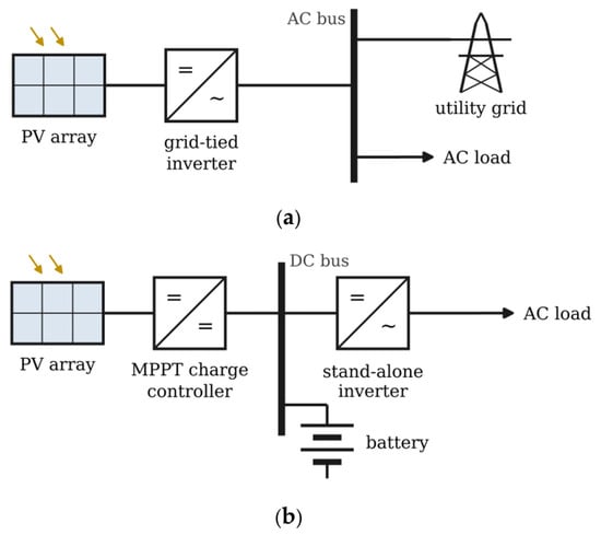
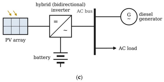
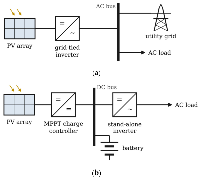
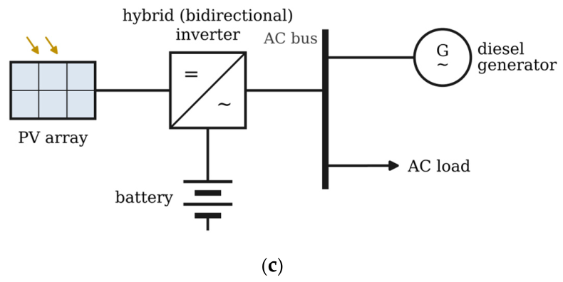
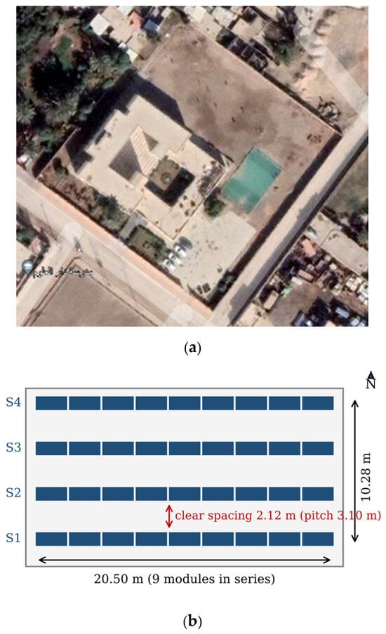
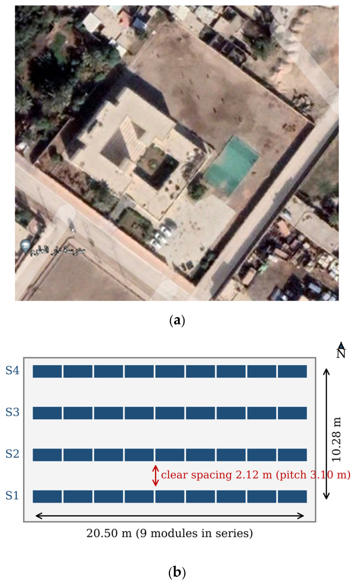
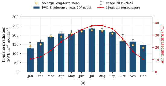
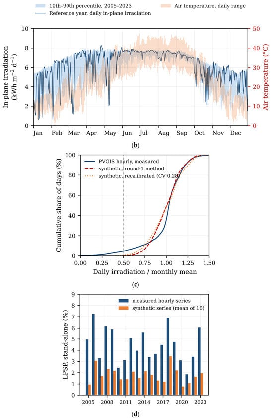
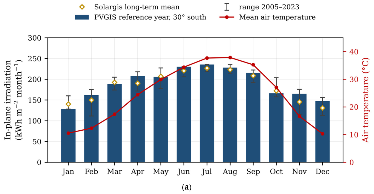
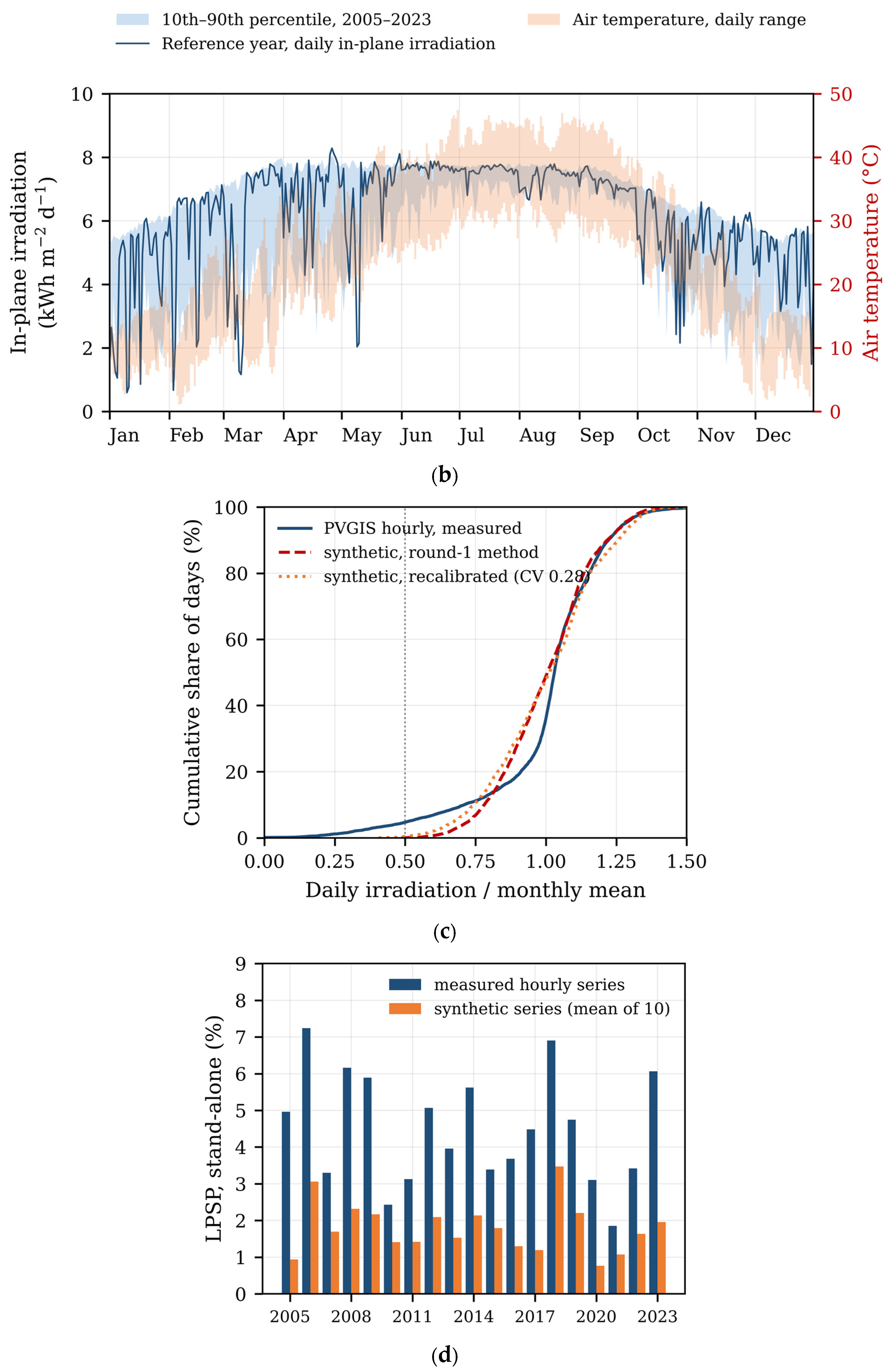
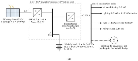
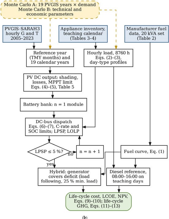
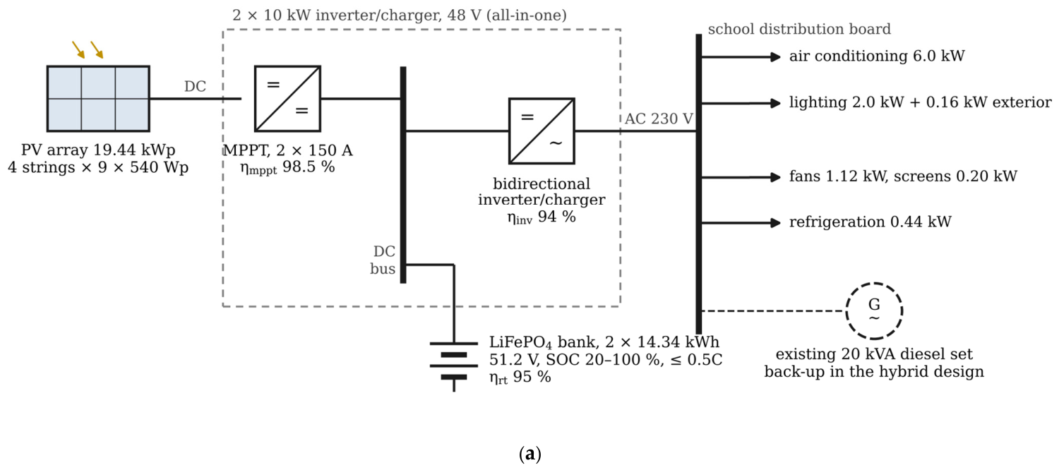
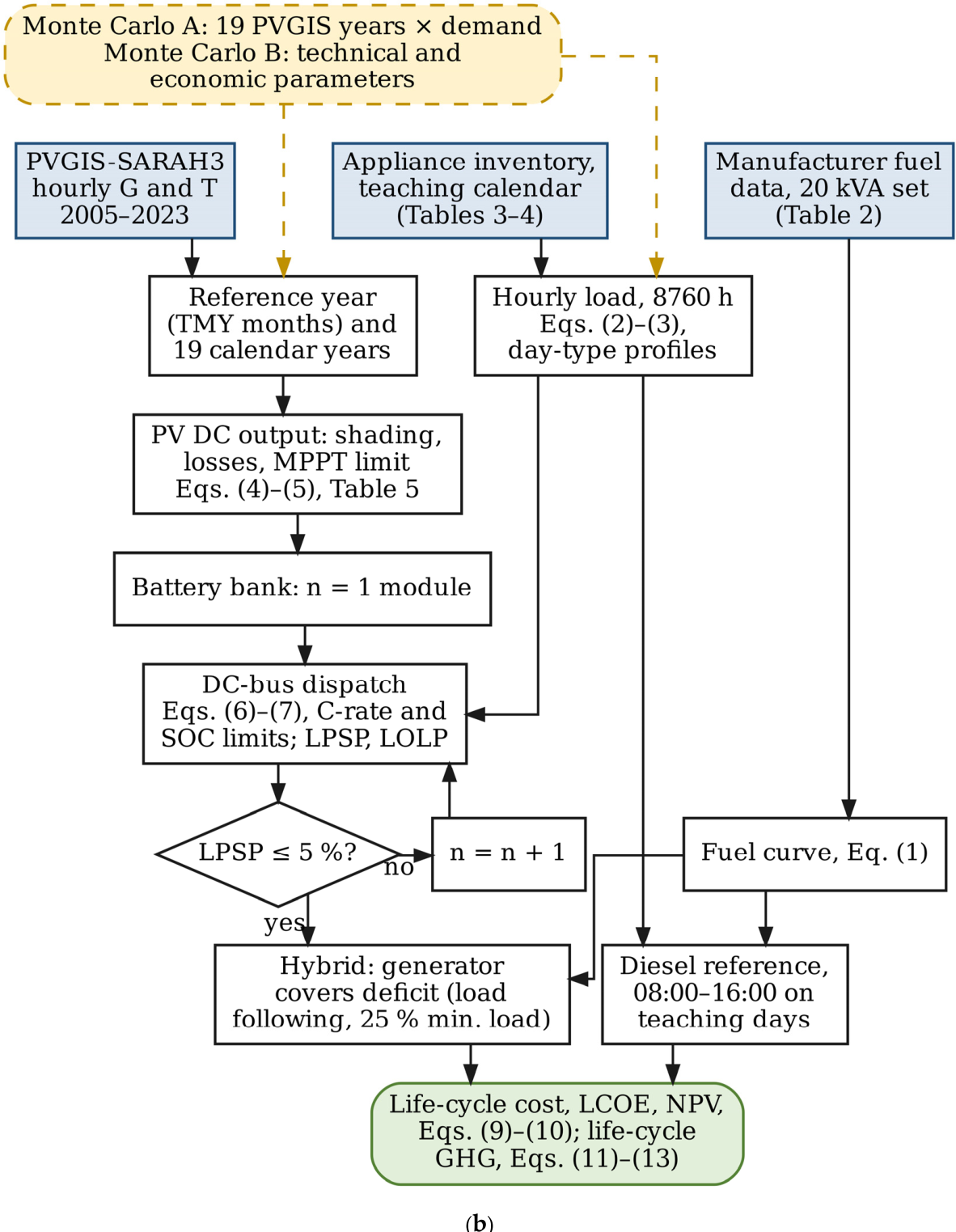
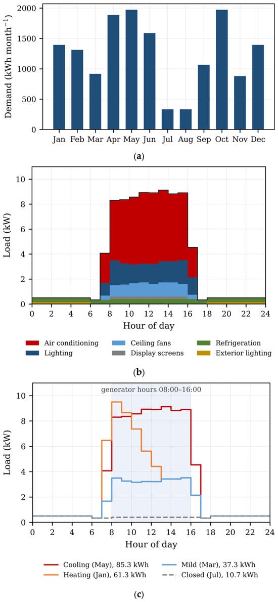
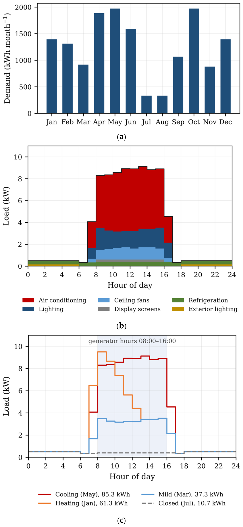
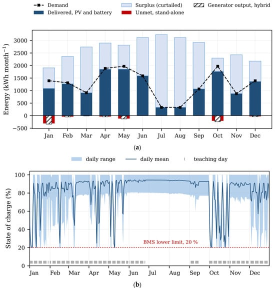
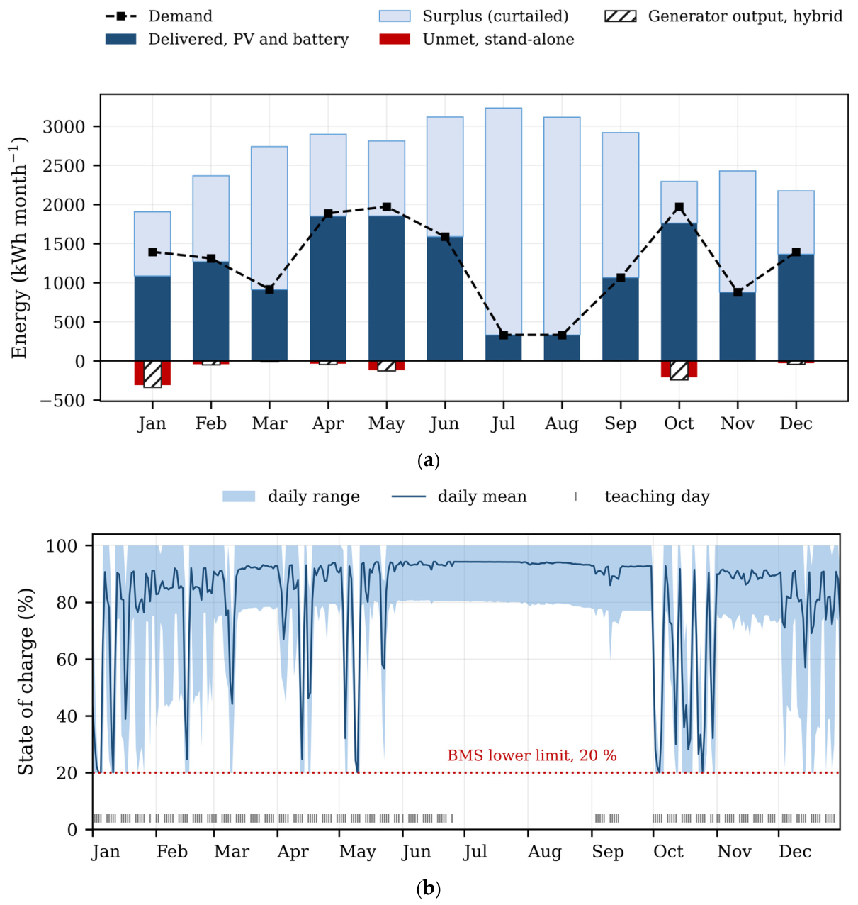
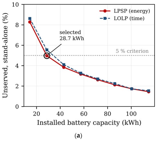
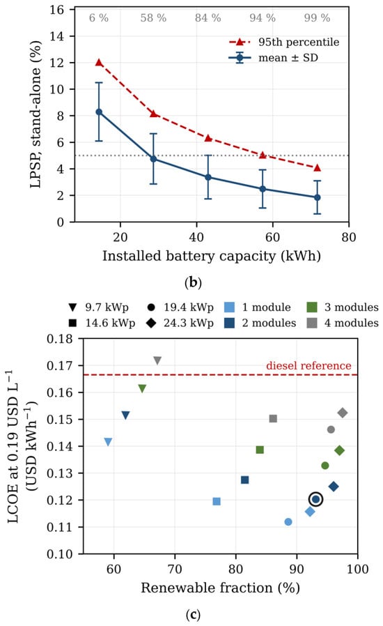
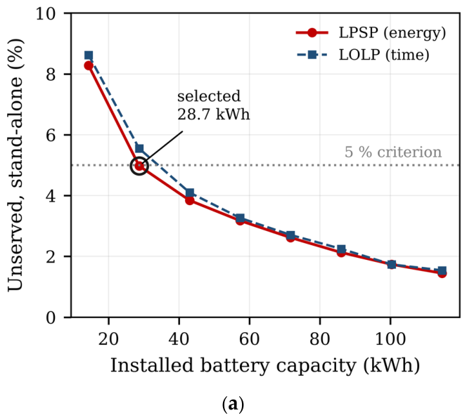
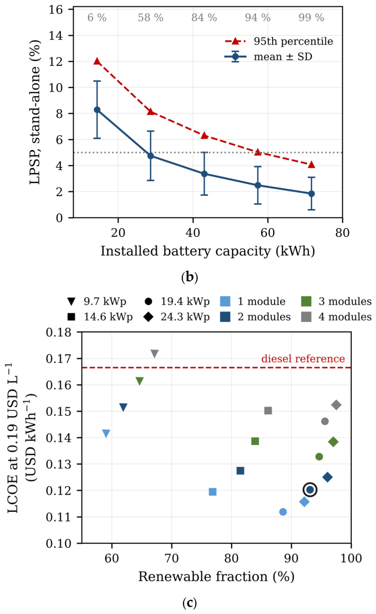
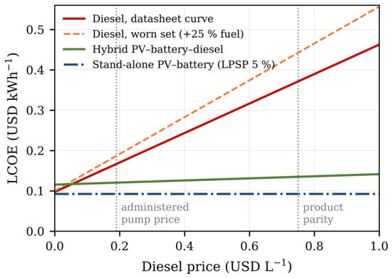
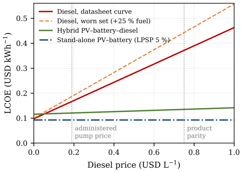
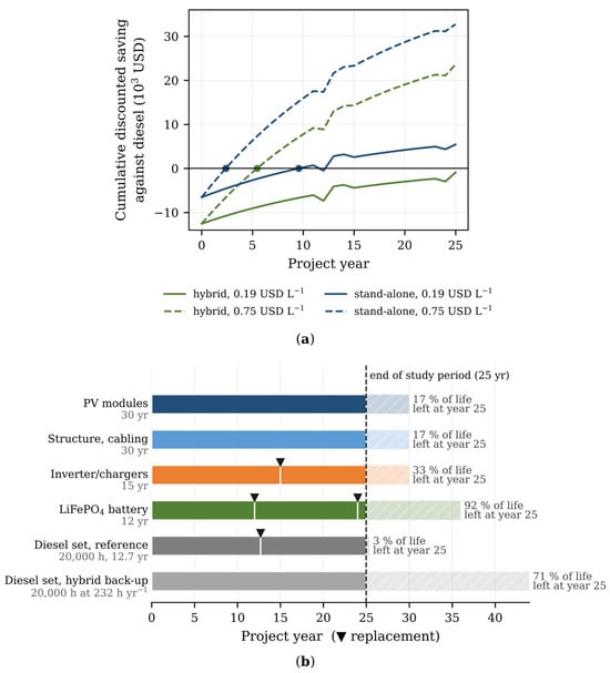
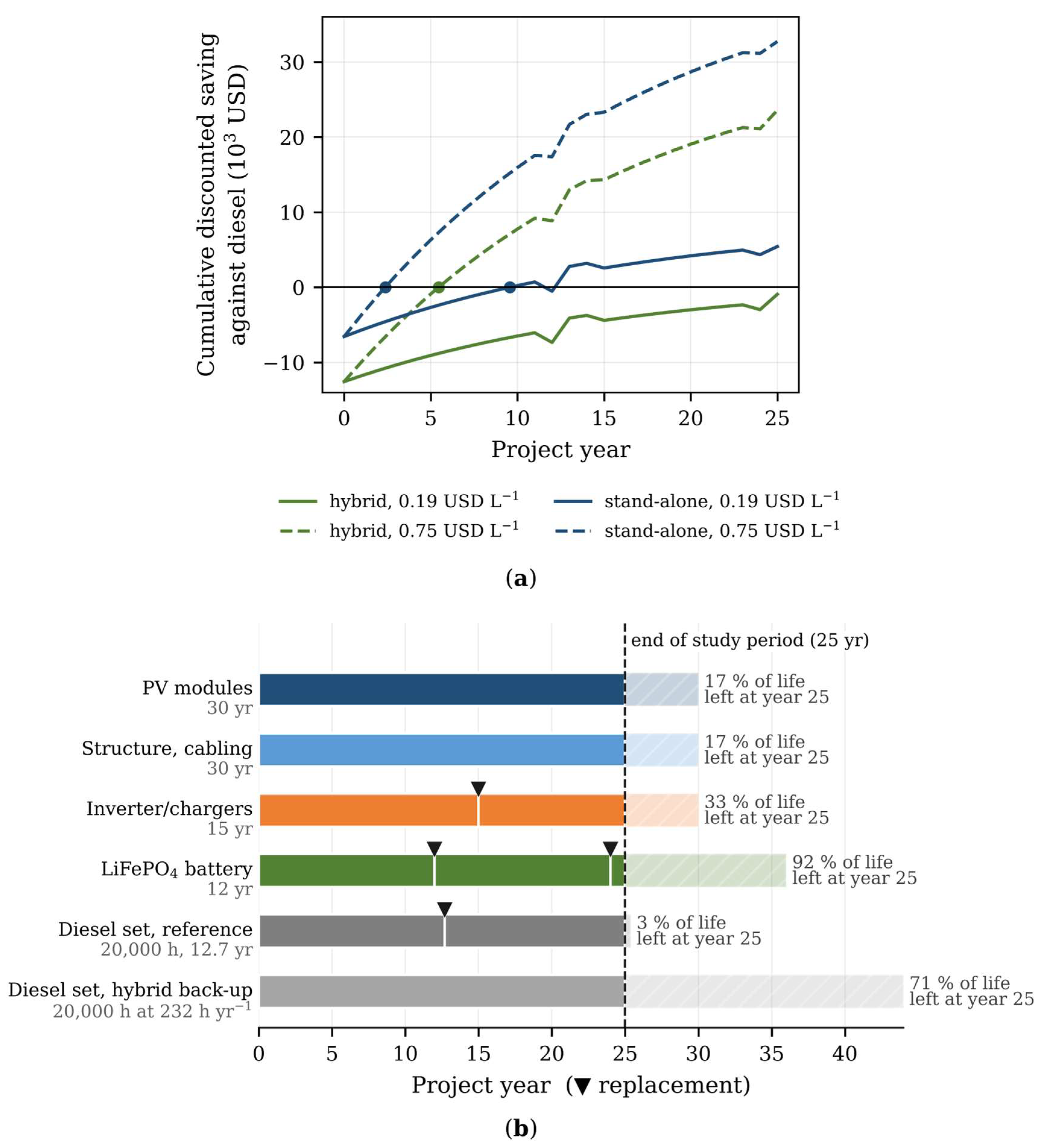
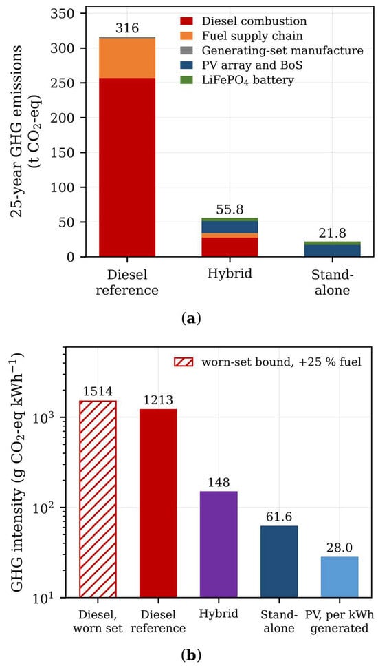
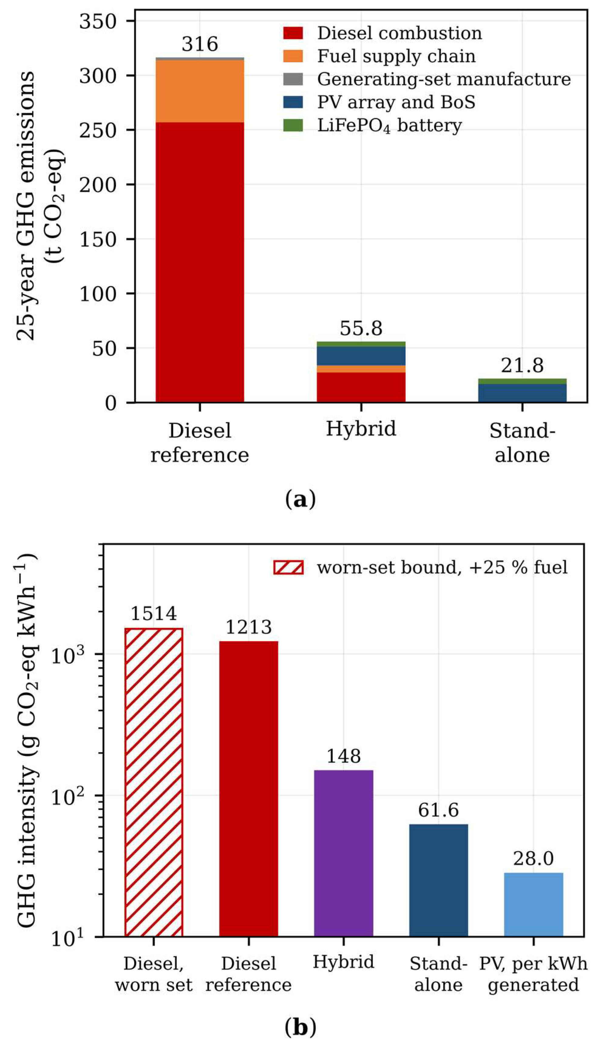
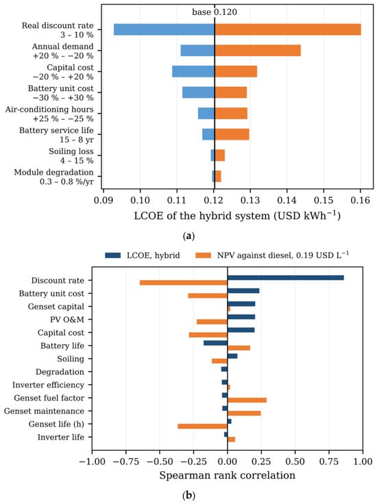
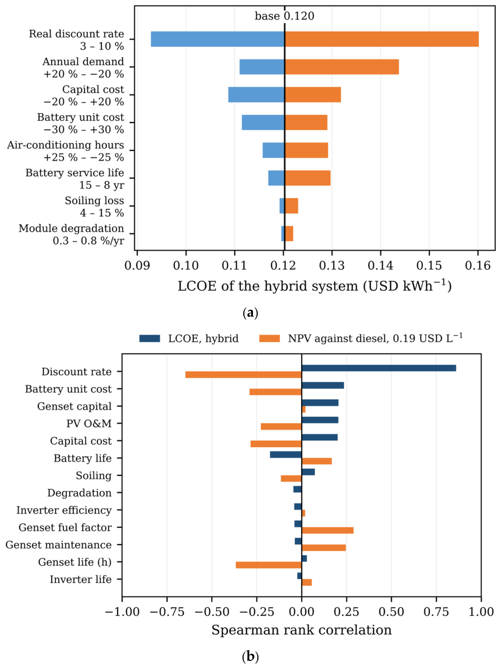

Disclaimer/Publisher’s Note: The statements, opinions and data contained in all publications are solely those of the individual author(s) and contributor(s) and not of MDPI and/or the editor(s). MDPI and/or the editor(s) disclaim responsibility for any injury to people or property resulting from any ideas, methods, instructions or products referred to in the content. |
© 2026 by the authors. Licensee MDPI, Basel, Switzerland. This article is an open access article distributed under the terms and conditions of the Creative Commons Attribution (CC BY) license.