Robust Flexibility Aggregation of Virtual Power Plants Considering Commercial Constraints and Temporal Decoupling

Abstract

Driven by the accelerated transition toward low-carbon power systems, Virtual Power Plants (VPPs) have emerged as an essential paradigm for aggregating distributed energy resources (DERs). Consequently, accurately characterizing the aggregated multi-dimensional feasible region (FR) of VPPs is imperative to facilitate coordinated dispatch and support the secure and economic operation of the upstream grid. However, constrained by the neglect of retail price elasticity, the inability to quantify subjective user default risks, and the computational complexity of high-dimensional inter-temporal coupling, traditional purely physical modeling approaches often overestimate flexibility and suffer from the curse of dimensionality. To address these issues, a multi-dimensional robust FR characterization framework for VPPs considering commercial constraints and inter-temporal decoupling is proposed in this paper. First, a dual-coupled VPP aggregation model integrating physical boundaries and commercial retail mechanisms is formulated. Second, a robust uncertainty budget mapping mechanism based on user credit profiles is developed to comprehensively quantify the dual uncertainties of meteorological randomness and human behavioral defaults. Finally, a projection-based FR characterization method utilizing epigraph theory and Lyapunov optimization is proposed to decouple complex inter-temporal constraints with single-round VPP-ISO coordination and an iterative internal boundary-construction procedure. Simulation results on a modified 33-node active distribution network verify the effectiveness of the proposed framework.

1. Introduction

With the accelerated transition toward low-carbon power systems, Virtual Power Plants (VPPs) have emerged as an essential technical paradigm for aggregating distributed energy resources (DERs), such as distributed generation, flexible loads, and energy storage systems (ESS) [1,2,3]. Quantifying the collective adjustable capacity of DERs through flexibility aggregation is the foundation for facilitating coordinated dispatch between VPPs and the transmission system. Normally, the aggregated flexibility is mathematically characterized via feasible region (FR) characterization at the point of common coupling (PCC) [4,5,6]. Accurate FR characterization provides an explicit operation boundary of VPPs for the independent system operator (ISO), which guarantees the security and stability of the power grid [7].

Currently, extensive research is devoted to quantifying VPP flexibility based on idealized hardware boundaries. In this context, flexibility aggregation evaluates the total adjustable capacity of DERs, which is subsequently characterized mathematically as the aggregated FR. For instance, a geometric approach was proposed in [8] to construct the aggregated FR of thermostatically controlled loads. In [9], zonotopes were utilized to approximate the aggregation of energetic flexibility for DERs. Meanwhile, an exact formulation and approximate models for the aggregate FR of DERs were developed in [10] to provide explicit boundaries for grid operators. Furthermore, a projection-based approach was applied in [11] to calculate the capability of DER aggregation. However, these conventional aggregation methodologies predominantly rely on idealized physical boundaries, which assumes that DERs strictly execute dispatch commands without conditional execution costs [12]. First, these models neglect the retail price elasticity mechanism, which dynamically alters the actual adjustable capacity of end-users. Second, they fail to account for rigid inter-temporal limitations imposed by commercial contracts, such as minimum response duration and maximum call frequency. Consequently, the theoretically derived FR often deviates from practical commercial operations, leading to an overestimation of flexibility.

In addition to physical boundaries, the inherent uncertainties of DERs significantly affect the accuracy of the aggregated FR, which prompts studies on uncertainty quantification in VPP scheduling. In [13], a robust optimization framework was proposed to estimate the active and reactive power boundaries of a VPP under operational uncertainties. In [14], a robust approach to chance-constrained optimal power flow was designed to mitigate the risks associated with renewable generation. Meanwhile, in [15], a Gaussian Mixture Model was employed to characterize the complex uncertainty distributions of renewable outputs in power systems. However, these existing uncertainty quantification techniques concentrate heavily on the objective meteorological randomness of renewable energy generation [16]. A significant operational risk in actual VPP scheduling stems from the subjective behavioral default of demand-side resources. Traditional methods fail to incorporate user execution reliability and credit default risks. Consequently, the theoretically derived FR often leads to severe dispatch violations and subsequent financial losses during actual execution due to user non-compliance.

Furthermore, intense inter-temporal coupling is introduced to the VPP system by both the physical state of charge (SOC) limits of ESS and the strict time clauses within commercial contracts. In [17], the aggregate flexibility of VPPs with temporal coupling constraints was modeled using an iterative optimization algorithm. In [18], the temporal-coupled FR of active distribution networks was characterized through an analytical method. In [19], a solution method for VPP dynamic FR based on the decoupling of coupling constraints was proposed to improve computational efficiency. However, the cross-period dependency expands the multi-dimensional FR into a highly complex, high-dimensional space [20]. Traditional aggregation algorithms, which often rely on iterative optimization or polyhedral vertex enumeration, become computationally intensive. Such methods struggle to overcome the curse of dimensionality, which makes it difficult to satisfy the timeliness requirements of single-round coordinated dispatch between the VPP and the transmission network in day-ahead and real-time markets.

To address these issues, a multi-dimensional robust FR characterization framework for VPPs considering commercial constraints and inter-temporal decoupling is proposed in this paper. First, operational constraints of heterogeneous DERs and retail price elasticity are integrated to formulate a dual-coupled VPP aggregation model. Then, a robust uncertainty budget mapping mechanism based on user credit profiles is developed to quantify the dual uncertainties of meteorological randomness and human behavior. Finally, an applicable projection-based FR characterization method is formulated, which utilizes epigraph theory and Lyapunov optimization to decouple the high-dimensional inter-temporal constraints.

The proposed framework makes three specific contributions. First, it proposes a physical–commercial dual-coupled VPP aggregation model that integrates distributed-energy-resource physical limits, retail-price elasticity, and commercial contract clauses, correcting the flexibility overestimation caused by purely physical aggregation. Second, it develops a credit-driven robust uncertainty-quantification mechanism that maps user default moments and correlations into a probabilistic reserve margin, covering both meteorological randomness and behavioral non-compliance. Third, it establishes an epigraph-based dimensionality-reduction and Lyapunov temporal-decoupling algorithm that constructs the feasible-region boundary with a quantified approximation error. The framework does not claim a fundamentally new mixed-integer programming solver. A quantitative comparison with the closest time-domain coupling methods is provided in Section 5.

The remainder of this paper is organized as follows: Section 2 details the dual-coupled modeling of physical and commercial constraints for heterogeneous DERs. Section 3 presents the dual uncertainty quantification integrating user credit profiles. The theoretical decoupling of inter-temporal constraints and the applicable FR projection algorithm are elaborated in Section 4. Section 5 validates the effectiveness of the proposed framework through case studies. Section 6 concludes the paper.

2. The Modeling of VPPs Considering Physical and Commercial Coupling

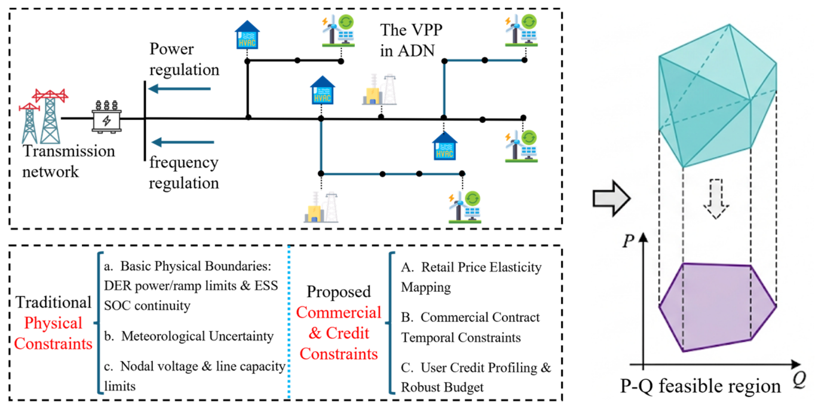
The feasible region of a VPP is determined by the physical constraints of the aggregated DERs. In practical electricity markets, however, the actual regulation capability is also restricted by the economic willingness of terminal users and by the temporal clauses of commercial contracts. This section formulates a dual-coupled aggregation model that combines physical boundaries with the retail-price mechanism and the commercial contract constraints.The overall framework of this coupled physical and commercial FR model for VPPs is illustrated in Figure 1.

Figure 1. Schematic of the coupled physical and commercial FR model for VPPs.

Figure 1. Schematic of the coupled physical and commercial FR model for VPPs.

2.1. Basic Physical Constraints of Heterogeneous DERs

The physical boundaries of a VPP are determined by the heterogeneous DERs it aggregates, which exhibit distinct control characteristics and energy coupling mechanisms. These primarily include ESS, renewable energy sources (RES), and interruptible loads (ILs) [21].

For an ESS unit, the operational state is constrained by bidirectional charge/discharge power limits, ramp rates, and the inter-temporal SOC continuity equation:

$$P_t=P_t^{dis}-P_t^{ch}$$

(1)

$$0\le P_t^{ch}\le {\overline{P}}^{ch}, 0\le P_t^{dis}\le {\overline{P}}^{dis}$$

(2)

$$SO{C}_t=SO{C}_{t-1}+{\eta }^{ch}{P}_t^{ch}\Delta t-{\displaystyle \frac{1}{{\eta }^{dis}}}{P}_t^{dis}\Delta t$$

(3)

$$SO{C}_{min}\le SO{C}_t\le SO{C}_{max}$$

(4)

$$-R_{max}^{ES}\le P_t-P_{t-1}\le R_{max}^{ES}$$

(5)

where $P_t^{ch}$ and $P_t^{dis}$ denote the charging and discharging power at time $t$, respectively; ${\eta }^{ch}$ and ${\eta }^{dis}$ represent the corresponding conversion efficiencies; and $R_{max}^{ES}$ is the maximum allowable inter-temporal ramp rate.

For dimensional consistency, the ESS energy balance is written as $E_i{\mathit{SOC}}_{i,t+1}=E_i{\mathit{SOC}}_{i,t}+({\eta }_i^{\mathit{ch}}{P}_{i,t}^{\mathit{ch}}-P_{i,t}^{\mathit{dis}}/{\eta }_i^{\mathit{dis}})\Delta t$, where $E_i$ is in kWh, $P_{i,t}^{\mathit{ch}}$ and $P_{i,t}^{\mathit{dis}}$ are in kW, and $\Delta t$ is in hours. Dividing by $E_i$ gives ${\mathit{SOC}}_{i,t+1}={\mathit{SOC}}_{i,t}+({\eta }_i^{\mathit{ch}}{P}_{i,t}^{\mathit{ch}}-P_{i,t}^{\mathit{dis}}/{\eta }_i^{\mathit{dis}})\Delta t/E_i$. The energy capacity normalizes the energy increment and remains in every SOC bound; it is not removed from the physical problem.

For RES (e.g., distributed photovoltaic (PV) and wind generation), the output characteristics are modeled as unidirectional injections bounded by the predicted available power limit:

$$0\le P_t^{RES}\le {\widehat{P}}_t^{RES}$$

(6)

$$|P_t^{RES}-P_{t-1}^{RES}|\le R_{max}^{RES}$$

(7)

where ${\widehat{P}}_t^{RES}$ represents the forecasted theoretical maximum generation.

For traditional ILs, the physical model restricts the continuous adjustment range within fixed power bounds. For deferrable loads (e.g., industrial batch production processes), a total energy conservation constraint must be satisfied over the scheduling horizon:

$${\underset{\_}{P}}^{load}\le P_t^{load}\le {\overline{P}}^{load}$$

(8)

$${\displaystyle \sum _{t=1}^T{P}_t^{load}}\Delta t=E_{req}$$

(9)

The aforementioned models establish the theoretical physical regulation envelope, assuming the absence of commercial contract limitations and economic elasticity.

2.2. Dynamic Capacity Mapping via Retail Price Elasticity

In practical demand response (DR) programs, the adjustable capacity of commercial and industrial users is not a static hardware parameter but an elastic function dependent on price incentive levels. Establishing a dynamic mapping mechanism between price signals and regulation capacity is essential for accurately evaluating the commercial flexibility of the VPP.

The characteristics of demand response are rigorously represented by the Retail Price Elasticity Matrix [22]. The diagonal elements represent self-elasticity (${\epsilon }_{t,t}$), measuring the direct load reduction effect in response to price increments in the current period (typically negative). The off-diagonal elements represent cross-elasticity (${\epsilon }_{t,k}$), quantifying the load-shifting spillover effect across different periods (typically positive).

Let ${\lambda }_t$ be the nodal marginal price or DR compensation rate at time $t$, ${\lambda }_t^0$ be the baseline price, and $P_{j,t}^{load,0}$ be the baseline load of user $j$. Driven by price incentives, the elastic load profile $P_{j,t}^{load}$ is formulated as follows:

$$P_{j,t}^{load}=P_{j,t}^{load,0}\left[1+{\epsilon }_{t,t}{\displaystyle \frac{{\lambda }_t-{\lambda }_t^0}{{\lambda }_t^0}}+{\displaystyle \sum _{k\ne t}{\epsilon }_{t,k}}{\displaystyle \frac{{\lambda }_k-{\lambda }_k^0}{{\lambda }_k^0}}\right]$$

(10)

Defining the price variation rate vector as $\rho$, where ${\rho }_k=({\lambda }_k-{\lambda }_k^0)/{\lambda }_k^0$, the upper limit of the downward active power regulation capacity $\Delta P_{j,t}^{max,\rho }$ stimulated by economic incentives is determined by the following:

$$\Delta P_{j,t}^{max,\rho }=P_{j,t}^{load,0}-P_{j,t}^{load}=-P_{j,t}^{load,0}{\displaystyle \sum _{k=1}^T{\epsilon }_{t,k}}{\rho }_k$$

(11)

Consequently, the physical constraints in the VPP scheduling model are reformulated as dynamic constraints subject to price incentives:

$$0\le \Delta P_{j,t}^{down}\le \min (\Delta P_{j,t}^{max,\rho },{\overline{P}}_j^{contract})$$

(12)

where ${\overline{P}}_j^{contract}$ denotes the maximum downward limit permitted by equipment or network capacities. This constraint mechanism reveals that when price incentives are insufficient (${\rho }_k\approx 0$), the computed regulation FR contracts toward zero. Consequently, insufficient price incentives restrict the regulation FR toward zero. Conversely, significant peak-price stimulation substantially expands the multi-dimensional FR space, which mitigates the overestimation characteristic of purely physical models.

2.3. Integration of Commercial Contract Temporal Constraints

In VPP operations, resource dispatch is governed not only by physical ramp rates but also by strict commercial contract terms, which impose strong temporal coupling constraints. A binary state variable $u_{j,t}\in \{0,1\}$ is introduced to indicate whether device $j$ is activated at time $t$.

Notice Time Constraint: A minimum notice time ${\tau }_{notice}$ must be satisfied between the issuance of the dispatch instruction $I_{j,t}\in \{0,1\}$ and the actual resource response. This delay constraint is formulated as follows:

$$u_{j,t}\le I_{j,t-{\tau }_{notice}}$$

(13)

This constraint ensures the translation of flexibility from physically achievable bounds to commercially compliant operations.

Call Duration Constraint: Once a resource is activated, it must comply with the minimum ($T_{min}$) and maximum ($T_{max}$) continuous operation duration specified in the contract:

$${\displaystyle \sum _{k=t}^{t+T_{min}-1}{u}_{j,k}}\ge T_{min}(u_{j,t}-u_{j,t-1}), \forall t$$

(14)

$${\displaystyle \sum _{k=t}^{t+T_{max}}{u}_{j,k}}\le T_{max}, \forall t$$

(15)

Call Frequency and Active Window Constraints: To enforce the maximum daily call frequency $N_{max}^{daily}$ and the permissible active time window ${\mathcal{T}}_{active}$, the following constraints are formulated:

$${\displaystyle \sum _{t=2}^{T_{day}}\max }(0,u_{j,t}-u_{j,t-1})\le N_{max}^{daily}$$

(16)

$$u_{j,t}=0, \forall t\notin {\mathcal{T}}_{active}$$

(17)

By embedding these temporal variables and logic limitations into the sequential update framework, the underlying physical envelope is upgraded into a multi-dimensional commercial flexibility hyperspace.

2.4. Reactive-Power Capability of DER Inverters and Network Constraints

The P-Q feasible regions reported in this paper are determined jointly by the inverter apparent-power capability of the DERs and the operating constraints of the active distribution network. The following formulation also fixes the PCC sign convention used in the numerical study.

Assumption 1

(sign convention). At the PCC and every DER node, $P>0$ denotes net injection into the upstream grid and $P<0$ denotes net withdrawal. Reactive power follows the same convention. For a negative active-power boundary coordinate we report $P^{\min }<0$ and the guaranteed net-withdrawal magnitude $\left|P^{\min }\right|$. The ambiguous phrase “upper active-power limit” is not used for negative $P$.

$$P_{\mathit{pcc}}(t)>0: \mathit{net} \mathit{injection}, P_{\mathit{pcc}}(t)<0: \mathit{net} \mathit{withdrawal}$$

(18)

For each DER-connected inverter i (PV, WT, IL, and ESS), the apparent-power capability is as follows:

$$P_i{(t)}^2+Q_i{(t)}^2\le {(S_i^{\max })}^2, \forall i\in \mathcal{D}, \forall t$$

(19)

$$-Q_i^{\max }\le Q_i(t)\le Q_i^{\max }, Q_i^{\max }=S_i^{\max }\sin (\arccos {\phi }_i^{\min })$$

(20)

$$-|P_i(t)|\tan {\phi }_i^{\max }\le Q_i(t)\le |P_i(t)|\tan {\phi }_i^{\max }$$

(21)

The interconnection of the VPP resources is represented by the linearized DistFlow model. For each branch (n,m) and phase p,

$$P_{nm}^p(t)={\displaystyle \sum _{k\in {\mathcal{C}}_m}{P}_{mk}^p}(t)+p_m^p(t), Q_{nm}^p(t)={\displaystyle \sum _{k\in {\mathcal{C}}_m}{Q}_{mk}^p}(t)+q_m^p(t)$$

(22)

$$V_m^p(t)=V_n^p(t)-{\displaystyle \frac{r_{nm}{P}_{nm}^p(t)+x_{nm}{Q}_{nm}^p(t)}{V_0}}$$

(23)

$$V_{\min }\le V_n^p(t)\le V_{\max }, {(P_{nm}^p(t))}^2+{(Q_{nm}^p(t))}^2\le {(S_{nm}^{\max })}^2$$

(24)

where $S_i^{\max }$ is the rated apparent power of inverter i, $Q_i^{\max }$ is its reactive-power limit, ${\phi }_i^{\min }$ is the minimum power factor, $r_{nm}$ and $x_{nm}$ are the branch resistance and reactance, and $V_n^p$ is the phase-p voltage at node n. The apparent-power and power-factor limits are enforced for both charging and discharging operating points.

Equation (19) is the exact disk $P_{i,t}^2+Q_{i,t}^2\le S_i^2$. The reported MILP uses the regular inscribed polygon $\cos {\theta }_l{P}_{i,t}+\sin {\theta }_l{Q}_{i,t}\le S_i\cos (\pi /n_s)$, ${\theta }_l=2\pi l/n_s+{\theta }_0$, $l=0,\dots ,n_s-1$. The reported mesh is $n_s=96$. The maximum radial error is $e_{\mathit{rad},i}=S_i[1-\cos (\pi /n_s)]$; for $S_{\max }=0.50$ MVA it is $2.68\times {10}^{-4}$ MVA. Repeating the boundary construction with $n_s=192$ changes the P-Q boundary by $2.01\times {10}^{-4}$ MW. Equation (24) and the power-factor sectors use the same inscribed construction.

The error introduced by the MILP approximation is quantified in two complementary ways. The first is analytical, because the inscribed polygon gives a radial bound. The second is numerical, because the boundary computation is repeated with a doubled sector count and the difference between successive P-Q boundaries is reported together with the sector count used for each boundary.

For inverter $i$, the exact capability is $P_{i,t}^2+Q_{i,t}^2\le S_i^2$. The inscribed polygon is an inner approximation, whereas OPA is an outer approximation of the projection of the discretized set. Therefore $\mathrm{\Pi }({\mathcal{F}}_{\mathit{in}})\subseteq \mathrm{\Pi }({\mathcal{F}}_{\mathit{exact}})$ and $\mathrm{\Pi }({\mathcal{F}}_{\mathit{in}})\subseteq {\mathcal{P}}_{\mathit{OPA}}$, but no net sign is claimed for the distance between ${\mathcal{P}}_{\mathit{OPA}}$ and the exact projection.

The PCC P-Q feasible region ${\mathcal{R}}_t$ is defined as the projection of the coupled physical–commercial model onto the PCC power variables. Since the distribution network is operated in a balanced manner, the single-phase equivalent of the DistFlow model is used; the three-phase connection data only allocate the single-phase ratings. The voltage limits and the branch thermal limits are denoted by $V_{\min }$, $V_{\max }$, and $S_{nm}^{\max }$, respectively.

3. Uncertainty Quantification Incorporating Renewable Fluctuations and User Credit Profiling

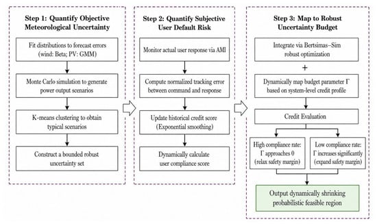
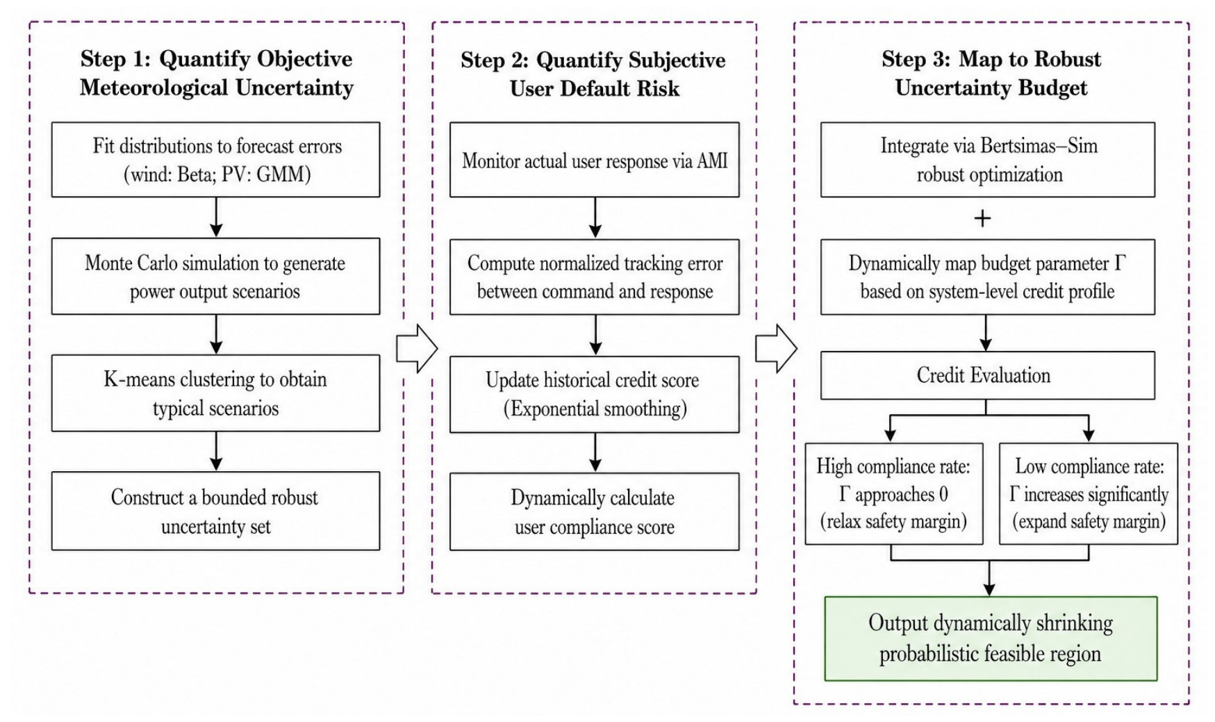
Traditional robust FR models primarily focus on the objective uncertainty of renewable energy generation caused by meteorological variations. However, a significant operational risk in actual VPP scheduling stems from the subjective behavioral default of demand-side resources. To construct a probabilistically valid FR, a dual uncertainty quantification framework is proposed to address both objective meteorological randomness and subjective user credit risks, as depicted in Figure 2.

Figure 2. Flowchart of the dual uncertainty quantification framework incorporating meteorological fluctuations and user credit profiling.

3.1. Scenario-Based Uncertainty Quantification for Renewable Generation

The uncertainty of wind and PV generation is quantified by a scenario-based method. Wind forecast errors are modeled by a finite mixture of Beta distributions, and PV forecast errors are represented by a Gaussian mixture model. A large set of renewable output scenarios is first generated by Monte Carlo sampling and then reduced by K-means clustering to a set of representative scenarios. The temporal and spatial correlations of the forecast errors are embedded in a covariance matrix ${\Sigma }^{\mathit{meteo}}$.

The robust uncertainty set is constructed around the typical scenarios as follows:

$${\mathcal{U}}^{\mathit{meteo}}=\{\xi \in {ℝ}^{N_{g}T}: \Vert \xi {\Vert }_{\infty }\le 1, \Vert \xi {\Vert }_1\le {\mathrm{\Gamma }}^{\mathit{meteo}}\}$$

(25)

Here, the number of renewable units and the dispatch horizon define the dimension of the normalized forecast-error vector. The meteorological budget is set to 8 for the 24 h case study. The nominal forecast-error scale is obtained from the fitted distributions, and the covariance matrix is defined below.

$${\Sigma }_{(i,t),(k,s)}^{\mathit{meteo}}={\sigma }_i(t){\sigma }_k(s){\rho }_{ik}\exp \left(-{\displaystyle \frac{|t-s|}{\tau }}\right)$$

(26)

The meteorological budget is calibrated from the fitted scenario distribution at the prescribed coverage level. The Monte Carlo study then reports the resulting out-of-sample violation probability and its Wilson confidence interval; this empirical coverage assessment is not presented as a distribution-free Bertsimas–Sim probability guarantee.

No additional closed-form probability inequality is invoked here; the target coverage is assessed by the fitted-scenario calibration and the out-of-sample Monte Carlo protocol described in Section 5.3.

For the reported case, the budget is selected to target 98% scenario coverage over the 24 h horizon.

3.2. Dynamic Quantification of User Commitment Score

To quantitatively evaluate the execution reliability of flexible loads, a Commitment Score (CS) ($C_j$) metric is introduced. This index assesses the actual output relative to the market contract baseline.

Let the cleared instruction and the AMI-measured response of user j at time t define the $\epsilon$-regularized normalized tracking error shown below.

$$e_j(t)={\displaystyle \frac{|P_j^{\mathit{act}}(t)-P_j^{*}(t)|}{|P_j^{*}(t)|+\epsilon }}, \epsilon ={10}^{-3} p.u.$$

(27)

To capture the historical memory effect of user compliance, the CS is dynamically updated via exponential smoothing:

Where $\alpha$ in (0,1) is the smoothing coefficient and $C_j\left(0\right)$ is the initial score. The score is used as a monotone operational reliability index rather than as a calibrated probability of default.

$$C_j(t+1)=\alpha C_j(t)+(1-\alpha )\left(1-\min (1,{\overline{e}}_j^P(t))\right)$$

(28)

Here, the smoothing coefficient governs the memory assigned to past compliance. A score close to one indicates consistent delivery, whereas a lower score indicates weaker operational reliability. The probability statement for the robust boundary is provided by Theorem 1 rather than by the score itself.

3.3. Robust Uncertainty Budget Mapping via Credit Profiling

To integrate the credit metric into the robust optimization framework, the actual response of user j is modeled as the cleared response plus a bounded behavioral deviation:

$$P_j^{\mathit{act}}(t)=P_j^{*}(t)+{\xi }_j(t)\Delta P_j^{\max }, {\xi }_j(t)\in [-1,1]$$

(29)

where $\Delta P_j^{\max }$ is the maximum response deviation and ${\xi }_j(t)$ is a signed response-deviation variable. Negative values represent under-delivery, whereas positive values represent over-response or rebound within the dispatch interval. Because the optimization model does not contain a delay-state or delayed-input equation, response latency is not introduced as a separate parameter. Delayed and rebound behavior is reflected in the AMI-derived tracking errors and default moments rather than represented by an unsupported first-order lag.

For $\Delta P_j^{\max }=\left|{\kappa }_j\right|{\overline{\Delta P}}_j$, let $\Delta P_{(1)}^{\max }\ge \Delta P_{(2)}^{\max }\ge \cdots$ be the ordered caps. The worst admissible deviation in Equation (29) is the sum of the ${\mathrm{\Gamma }}_{\mathit{credit}}$ largest caps: ${\overline{\Delta P}}_{\mathrm{\Gamma }}={\displaystyle \sum _{r=1}^{{\mathrm{\Gamma }}_{\mathit{credit}}}\Delta }{P}_{(r)}^{\max }$. It is not the average cap. The integer form uses ${\displaystyle \sum _{k=0}^{{\mathrm{\Gamma }}_{\mathit{credit}}}\left(\begin{array}{c}J\\ k\end{array}\right)}$ admissible patterns.

In Equation (29), the realized response of user $j$ is written as $P_j^{\mathit{act}}(t)=P_j^{*}(t)+\Delta P_j^{\max }{\xi }_j(t)$, where $P_j^{*}(t)$ is the cleared instruction, $\Delta P_j^{\max }$ is the maximum signed response deviation, and ${\xi }_j(t)\in [-1,1]$ is a normalized signed deviation.

The probabilistic statement in Theorem 1 concerns the aggregate default count $S_D={\displaystyle \sum _j{D}_j}(t)$. A bound on $S_D$ alone does not control MW error unless each default is assigned a bounded deviation. With the model in Equation (29), the total continuous deviation satisfies ${\displaystyle \sum _j|}{d}_j(t)|\le {\displaystyle \sum _j{D}_j}(t){\overline{d}}_j(t)$, so a budget on ${\displaystyle \sum _j{D}_j}(t)$ bounds the weighted deviation set used by the feasibility check rather than an unbounded MW error.

Instead of assigning a static empirical budget, the credit budget is estimated from the default moments associated with the current portfolio credit profile. For a generic dispatch slot, let $D_j=\mathbb{I}(e_j>{\epsilon }_D)\in \{0,1\}$ denote the binary default indicator, where ${\epsilon }_D=0.05$ is the non-compliance threshold used for calibration. Define $D={[D_1,\dots ,D_N]}^{\top }$, $\mu =\mathbb{E}[1^{\top }D]$, and $\Sigma =\mathrm{Cov}(D)$. The moments are estimated from the 60-day AMI calibration records corresponding to the portfolio’s Commitment Score level. The capped robust budget is as follows:

Because the moments are finite-sample estimates, the Cantelli statement in Theorem 1 is conditional on the estimated mean and covariance. A 2000-sample day-block bootstrap over the 60 calibration days gives the 95% intervals for Γ_credit: [1.82, 2.18], [2.76, 3.00], and [3.81, 4.00] for CS = 0.92, 0.80, and 0.65. The corresponding 5th–95th moment-sensitivity ranges for the violation probability are 3.28–3.91%, 1.91–2.44%, and 0.86–1.32%. The 30 reserved days are used only for out-of-sample evaluation.

$${\mathrm{\Gamma }}^{\mathit{credit}}=\min \left\{N, \mu +\kappa \sqrt{1^{\top }\Sigma 1}\right\}, \kappa =\sqrt{{\displaystyle \frac{1-\delta }{\delta }}}$$

(30)

where $N$ is the number of aggregated users, $\delta$ is the target violation level, and $\kappa =\sqrt{(1-\delta )/\delta }$. The term $\mu$ is the expected number of defaults and $\sqrt{1^{\top }\Sigma 1}$ is the standard deviation of the aggregate default count. The cap ${\mathrm{\Gamma }}_{\mathit{credit}}\le N$ preserves a valid cardinality budget.

For a high-reliability portfolio, the mapped credit budget is small and the required reserve against default is correspondingly limited. For a portfolio with frequent defaults, the budget increases and the reported flexibility envelope contracts. This mechanism trades nominal adjustable capacity for a larger operational margin against behavioral uncertainty.

Theorem 1

(one-sided probabilistic guarantee under correlation). Let $D_j\in \{0,1\}$ be the default indicator defined above and let $S_D={\displaystyle \sum _{j=1}^N{D}_j}$. Then $\mathbb{E}[S_D]=\mu$ and $\mathrm{Var}(S_D)=1^{\top }\Sigma 1$. If ${\mathrm{\Gamma }}_{\mathit{credit}}$ is defined by Equation (30), Cantelli’s inequality with $\kappa =\sqrt{(1-\delta )/\delta }$ gives $\mathbb{P}(S_D>{\mathrm{\Gamma }}_{\mathit{credit}})\le \delta$ for any dependence structure. The guarantee requires valid estimates of the aggregate mean and covariance, but it does not require independent defaults.

4. Multi-Dimensional FR Characterization of VPPs via Dimensionality Reduction and Temporal Decoupling

The SOC dynamics of the ESS units and the duration clauses of the commercial contracts create inter-temporal coupling in the VPP. Dynamic aggregation strategies can improve flexible regulation ability [23]; however, the proposed method does not remove these physical dependencies; it uses virtual queues to construct a slot-wise decision rule while retaining hard per-slot feasibility constraints.

4.1. Dimensionality Reduction of VPP Aggregation Models via Epigraph Theory

Integrated scheduling models typically incorporate both main grid generation costs and internal VPP operation costs. Directly transmitting the operating states of numerous DERs to the main grid incurs communication congestion and raises privacy concerns. Based on epigraph theory, the internal cost variables of the VPP are eliminated from the system-level objective; the internal resource variables remain inside the VPP-internal feasibility block, which is never transmitted [24].

Assuming the comprehensive internal operation cost function of a VPP is $C_{vpp}(P_{internal,t})$, an auxiliary variable $e_{vpp,t}$ is introduced to represent the upper bound of this cost at time $t$. The original cost terms in the objective function are then substituted by this single variable, which maps the complex DER outputs and cost associations into a linear constraint space:

$$\min {\displaystyle \sum _{t=1}^T\left(Cos{t}_{grid,t}+e_{vpp,t}\right)}$$

(31)

$$C_{vpp}(P_{internal,t})\le e_{vpp,t}$$

(32)

$${\underset{\_}{c}}_{vpp,t}\le e_{vpp,t}\le {\overline{c}}_{vpp,t}$$

(33)

Through this equivalent epigraph substitution, the internal cost variables are eliminated from the objective function. The transmission grid dispatcher only needs to process the PCC power and the equivalent cost variable ${\gamma }_t$, which significantly reduces the dimensionality of the system-level optimization while preserving information privacy.

The complete primal model of the ISO-level problem is as follows:

$$\min {\displaystyle \sum _{t=1}^T\left[{\lambda }_t{P}_{\mathit{pcc}}(t)\Delta t+{\gamma }_t\right]}$$

(34)

$${\gamma }_t\ge c_t(x_t), \forall t$$

(35)

$${\mathcal{G}}_t(P_{\mathit{pcc}}(t),{\gamma }_t)\le 0, x_t\in {\mathcal{X}}_t$$

(36)

where $c_t(x_t)$ is the comprehensive internal operation cost of the VPP at slot t, ${\lambda }_t$ is the day-ahead price, ${\mathcal{X}}_t$ is the internal feasible set of the VPP, and ${\mathcal{G}}_t$ represents the coupling constraints at the PCC. The ISO-level model contains only the PCC power and the equivalent cost variable at each slot, independently of the number of DERs; the internal resource variables remain in ${\mathcal{X}}_t$ and are never transmitted to the grid operator.

4.2. Temporal Decoupling of VPP Inter-Temporal Constraints Based on Lyapunov Optimization

After eliminating internal variables, the inter-temporal dependencies between consecutive periods must be addressed. This section introduces Lyapunov optimization to transform multi-period coupling constraints into a single-period virtual queue stability control problem, thereby achieving temporal decoupling [25].

Taking the ESS SOC constraint as an example, long-term energy balance requirements can be relaxed into average constraint conditions. First, a virtual queue $S_t$ is constructed to represent the deviation of the SOC from its target:

$$S_t=SO{C}_t-SO{C}_{target}$$

(37)

The cross-period state transition equation for this virtual queue is as follows:

$$S_{t+1}=S_t+\left({\eta }^{ch}{P}_t^{ch}-{\displaystyle \frac{1}{{\eta }^{dis}}}{P}_t^{dis}\right)\Delta t$$

(38)

where $S_t$ reflects the cumulative energy deviation from historical periods.

To maintain the strong stability of the queue, a quadratic Lyapunov function $L(S_t)={\displaystyle \frac{1}{2}}{S}_t^2$ is defined to measure the system deviation. The Lyapunov drift $\Delta L_t$ between adjacent periods is as follows:

$$\Delta L_t=L(S_{t+1})-L(S_t)={\displaystyle \frac{1}{2}}(S_{t+1}^2-S_t^2)$$

(39)

To balance queue stability (physical constraint satisfaction) and operational economy, a Drift-plus-Penalty (DPP) objective is formulated for a single period $t$:

$$\min \Delta L_t+V\cdot e_{vpp,t}$$

(40)

where $V$ is a trade-off parameter adjusting the weight between maintaining queue stability and minimizing current economic costs.

By substituting the state transition equation into $\Delta L_t$ and deriving its deterministic upper bound, the multi-period optimization problem collapses into an instantaneous decision problem dependent solely on the current state:

$${\min }_{P_t^{ch},P_t^{dis}} V\cdot e_{vpp,t}+S_t\left({\eta }^{ch}{P}_t^{ch}-{\displaystyle \frac{1}{{\eta }^{dis}}}{P}_t^{dis}\right)\Delta t$$

(41)

In this formulation, ESS decisions no longer require long-term forecasting for future periods ($t+1\dots T$). The current queue state $S_t$ inherently guides the charging and discharging actions to maintain equilibrium. Similarly, commercial contract limits, such as call duration constraints, are mapped into logical virtual queues. The Lyapunov optimization framework effectively transforms full-cycle temporal coupling into a localized static optimization governed by virtual queue lengths.

The commercial duration and frequency clauses are represented by three logical state variables: the continuous-call counter $H_j\left(t\right)$, the rest-period counter $R_j\left(t\right)$, and the rolling call-frequency counter $F_j\left(t\right)$. Their transitions and the binary activation decision $u_j\left(t\right)$ are defined below.

$$H_j(t+1)=u_j(t)[H_j(t)+1], H_j(t)\le T_j^{\max }$$

(42)

$$R_j(t+1)=[1-u_j(t)][R_j(t)+1], u_j(t)=1\Rightarrow R_j(t)\ge T_j^{\min ,\mathit{rest}}$$

(43)

$$F_j(t)={\displaystyle \sum _{k=t-23}^t{u}_j}(k), F_j(t)\le f_j^{\max }$$

(44)

The activation decision is additionally restricted by the active-window and notice-time clauses. These state variables are included in the Lyapunov function; the queue argument provides an asymptotic performance characterization, while the explicit counter limits enforce the commercial clauses at each slot.

$$\Delta L(t)+V\mathbb{E}[C(t)\mid Q(t)]\le B+V\mathbb{E}[C^{*}(t)]$$

(45)

$$\underset{T\to \infty }{\lim \sup }{\displaystyle \frac{1}{T}}{\displaystyle \sum _{t=1}^T\mathbb{E}}[Q(t)]\le {\displaystyle \frac{B+V{C}^{*}}{\epsilon }}$$

(46)

$$|{\mathit{SOC}}_s(t)-{\mathit{SOC}}_s^{\mathit{ref}}|\le {\displaystyle \frac{|Q_s(t)|}{E_s^{\mathit{cap}}}}$$

(47)

Theorem 2

(demonstrates Lyapunov near-optimality and is queue bound). Under the stated drift inequality and the assumed slack condition, the average queue bound and SOC-deviation relation hold. B is a finite quadratic-drift bound, V is a user-selected cost-versus-queue trade-off parameter, and $\epsilon$ is the slack rate. The policy has the standard asymptotic O(1/V)-O(V) trade-off; it does not establish exact finite-horizon optimality. Per-slot network, inverter, and operating limits are imposed explicitly in every slot-wise subproblem.

$$\min {\displaystyle {\displaystyle \sum _{t=1}^T}\left[\Delta L(t)+\mathrm{VC}(t)\right]}+{\alpha }_Q{\displaystyle \sum _s{\left[Q_s(T)\right]}^2}$$

(48)

4.3. Outer Progressive Approximation and Projection Algorithm for the Aggregated VPP FR

With temporal decoupling and variable dimensionality reduction achieved, the calculation of the VPP FR is localized to an independent time slot. The objective is to evaluate the multi-dimensional nonlinear set, which is subjected to price elasticity expansion and credit uncertainty budget constraints, and then to project it onto a lower-dimensional boundary (e.g., active power, reactive power, and cost).

4.3.1. Max–Min Dual Transformation and Big-M Linearization

To ensure that the reported boundary is robust to user default, the feasibility check is formulated as a bi-level max–min problem [26]. The outer level selects the worst admissible default realization within the credit budget, whereas the inner level adjusts the decoupled resources to minimize constraint violations for the requested PCC power. The associated feasibility-check problem is stated below.

For each fixed binary pattern, the continuous recourse problem is an LP. Strong duality implies zero duality gap. If $s\ge 0$ and $\lambda \ge 0$ are primal slacks and dual multipliers, then ${\lambda }^{\top }s=0$, so $s_k{\lambda }_k=0$ for every $k$. Equation (52) linearizes this primal–dual optimality condition with Big-M constants. The complete model is solved by branch and bound, not integer enumeration; no KKT statement is made for the mixed-integer problem as a whole.

The binary activation and default variables are not relaxed. The admissible default patterns satisfy $\mathcal{Z}(\mathrm{\Gamma })=\{z\in {\{0,1\}}^{JT}:{\displaystyle \sum _{j,t}{z}_{j,t}}\le \mathrm{\Gamma }\}$. If the default indicators are independent by user and slot, $N_{\mathrm{\Gamma }}={\displaystyle \sum _{k=0}^{\mathrm{\Gamma }}\left(\begin{array}{c}JT\\ k\end{array}\right)}$. In the reported four-IL daily-pattern case, $N_{\mathrm{\Gamma }}={\displaystyle \sum _{k=0}^{\mathrm{\Gamma }}\left(\begin{array}{c}4\\ k\end{array}\right)}$. The numerical solver uses CPLEX branch and bound.

In the corrected derivation, the primal feasibility constraints, dual feasibility constraints, and Equation (52) are imposed jointly. The binary pattern is selected by branch and bound. At an accepted boundary point, the fixed-pattern LP dual vector generates the feasibility cut; infeasible nodes do not generate cuts.

$${\max }_{\xi \in {\mathcal{U}}^{\mathit{credit}}} {\min }_{x\in {\mathcal{X}}_t}{\displaystyle \sum _{i\in \mathcal{D}}{v}_i}(x_i) s.t. \mathit{physical}\text{-}\mathit{commercial} \mathit{constraints}$$

(49)

Applying strong duality to the inner problem and introducing the explicit dual variables yields the single-level reformulation:

$${\max }_{\xi ,u} {\displaystyle \sum _m{\lambda }_m}{g}_m(\xi )+{\displaystyle \sum _n{\mu }_n}{h}_n(\xi )$$

(50)

$$0\le {\lambda }_m\perp [b_m-A_{m}x]\ge 0, 0\le {\mu }_n\perp [d_n-C_{n}x]\ge 0$$

(51)

$$b_m-A_{m}x\le M_1(1-z_m), {\lambda }_m\le M_3{z}_m$$

(52)

The Big-M constants are selected from explicit physical bounds: $M_1$ bounds the slack or capacity residual, $M_2$ bounds the applicable price spread, and $M_3$ bounds the associated dual multiplier. The constants are tightened before the solution; the adaptive update is used only as a numerical safeguard.

The per-slot MILP size is linear in the number of DERs and users, with $O(JT+IT)$ variables and the binary default and activation variables. Because general MILP solution time is not polynomial, the manuscript makes no polynomial-time claim; scalability is assessed empirically in Section 5.4.

To maintain numerical stability and avoid ill-conditioned formulations, the tightened Big-M bounds are used in the mixed-integer linear feasibility check.

4.3.2. Vertex Search and Outer Progressive Approximation

Leveraging the MILP verification engine, the equivalent polygonal projection boundary of the VPP is efficiently generated using the Vertex Search Method combined with the Outer Progressive Approximation (OPA) algorithm [27]:

Step 1: Initial Space Enclosure and Directional Scanning

Initialize a sufficiently large polygon ${\mathcal{P}}_0$ that entirely covers the feasible space on the target projection plane. Define a series of search direction vectors ${\xi }^{(i)}={[\cos {\theta }_i,\sin {\theta }_i]}^T$, and execute extreme vertex searches:

$${\max }_{x_{vpp}} {\xi }^{(i)T}\cdot x_{vpp}$$

(53)

Step 2: Violation Identification and Dichotomy Location

If an identified extreme vertex yields a non-zero objective in the MILP verification, the point lies outside the FR. A one-dimensional dichotomy search is then performed between this external infeasible point and a known internal feasible baseline to precisely locate the critical boundary point.

Step 3: Feasibility Cut Generation

At the identified boundary point, the optimal dual solution vector ${\mu }^{*}$ is extracted from the MILP output. A hyperplane, termed a “Feasibility Cut”, is generated based on the dual multiplier slopes:

$${\mu }^{*T}(x-x_{limit})\le 0$$

(54)

This cut truncates the unfeasible areas from ${\mathcal{P}}_0$.

Step 4: Adaptive Iteration and Convergence

The final output is an inequality representation of an outer approximation to the projected FR for the specified slot. Its accuracy is controlled by the angular resolution and bisection tolerance and is quantified in the numerical comparison.

Through this explicitly defined boundary condition, the ISO can execute global optimization without accessing the internal parameters of the VPP. This framework facilitates single-round coordinated dispatch between the VPP and the transmission grid. The projected boundary is an approximation of the true projection, and its accuracy is controlled by the bisection tolerance and the angular resolution through Theorem 3.

Theorem 3

(sampled projection-error bound). For a compact star-shaped sampled cross-section, the Hausdorff distance between the OPA boundary and the sampled radial projection satisfies $d_H(\partial {\mathcal{P}}_{\mathit{OPA}},\partial {\widehat{\mathcal{F}}}_{N_{\theta }})\le {ϵ}_b+R_{\max }(1-\cos (\Delta \theta /2))$. This bound refers to the sampled projection only. It does not bound the distance to the unsampled true projection unless an additional continuous-support assumption is imposed.

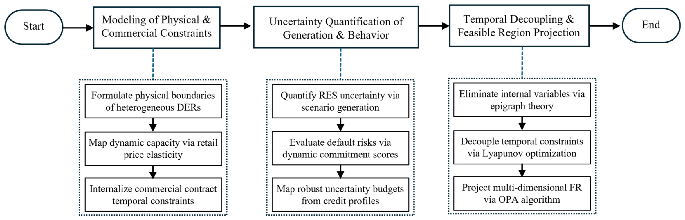
By integrating the physical–commercial constraint formulations, the dual uncertainty quantification, and the inter-temporal decoupling, the overall framework for characterizing the multi-dimensional robust FR is established, as illustrated in Figure 3.

Figure 3. Overall framework of the proposed multi-dimensional robust FR characterization.

Figure 3. Overall framework of the proposed multi-dimensional robust FR characterization.

5. Results

5.1. Testing System

To validate the proposed framework, numerical experiments are conducted on a modified 33-node medium-voltage active distribution network [28]. The nominal voltage is 12.66 kV and the base power is 10 MVA. Relative to the standard IEEE 33-bus feeder, DER units are connected at nodes 4, 5, 7, 8, 9, 11, 12, 13, 14, 17, 18, 20, 22, 23, 24, 27, 28, 30, and 31; the base load of nodes 9, 17, 23, and 31 is increased by 15%; and the fixed shunt elements are removed, as shown in Figure 4.

Figure 4. Topology of the modified 33-node active distribution network.

Figure 4. Topology of the modified 33-node active distribution network.

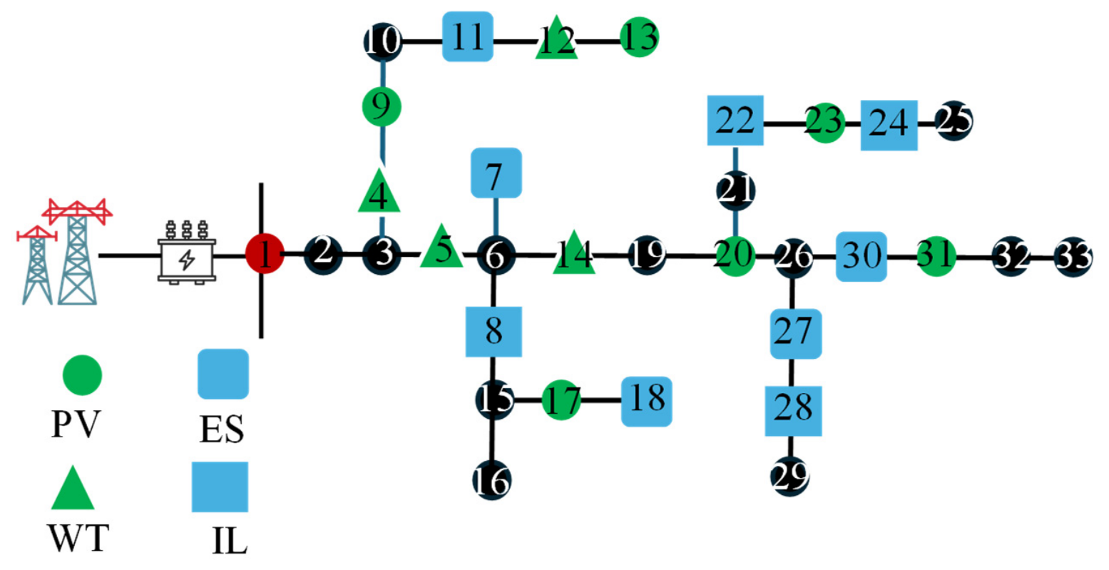
The VPP aggregates four distinct categories of DERs: distributed PV, wind turbines (WT), ILs, and ESS. The connection nodes, power factors, rated capacities, connection types, and operational parameters of the PV and WT units are given in Table 1, and those of the ILs and ESSs are provided in Table 2 and Table 3, respectively.

Table 1. Parameters of the distributed PV and WT units (revised; rated active-power and apparent-power capacities added).

Connect Node	DER Types	Power Factor	Rated Capacity (MW)	${\mathit{S}}_{\mathit{m}\mathit{a}\mathit{x}}$ (MVA)	Connection Type	Phases	Action Time
9, 13	PV	0.9	0.45 each	0.50	wye	a	<5 s
17, 20	PV	0.9	0.40 each	0.45	wye	b	<5 s
23, 31	PV	0.9	0.40 each	0.45	wye	c	<5 s
4, 5, 12, 14	WT	0.95	0.375 each	0.40	delta	ab, bc, ca	<5 s

Table 1. Parameters of the distributed PV and WT units (revised; rated active-power and apparent-power capacities added).

Connect Node	DER Types	Power Factor	Rated Capacity (MW)	${\mathit{S}}_{\mathit{m}\mathit{a}\mathit{x}}$ (MVA)	Connection Type	Phases	Action Time
9, 13	PV	0.9	0.45 each	0.50	wye	a	<5 s
17, 20	PV	0.9	0.40 each	0.45	wye	b	<5 s
23, 31	PV	0.9	0.40 each	0.45	wye	c	<5 s
4, 5, 12, 14	WT	0.95	0.375 each	0.40	delta	ab, bc, ca	<5 s

Table 2. Parameters of the interruptible loads (revised; apparent-power capacity expressed in kVA).

Connect Node	DER Types	Power Factor	${\mathit{S}}_{\mathit{m}\mathit{a}\mathit{x}}$ (kVA)	Connection Type	Action Time
8	IL	0.9	180 kVA	delta	<5 s
22	IL	0.9	200 kVA	delta	<5 s
24	IL	0.9	130 kVA	delta	<5 s
28	IL	0.9	100 kVA	delta	<5 s

Table 2. Parameters of the interruptible loads (revised; apparent-power capacity expressed in kVA).

Connect Node	DER Types	Power Factor	${\mathit{S}}_{\mathit{m}\mathit{a}\mathit{x}}$ (kVA)	Connection Type	Action Time
8	IL	0.9	180 kVA	delta	<5 s
22	IL	0.9	200 kVA	delta	<5 s
24	IL	0.9	130 kVA	delta	<5 s
28	IL	0.9	100 kVA	delta	<5 s

Table 3. Parameters of the energy storage systems (revised; energy capacity E in kWh, SOC limits in p.u., and distinct charge/discharge efficiencies ${eta}_{ch}$ and ${eta}_d$).

Connect Node	DER Types	Power Factor	${\mathit{P}}_{\mathit{m}\mathit{a}\mathit{x}}$/E (kW/kWh)	${\mathit{S}\mathit{O}\mathit{C}}_{\mathit{m}\mathit{i}\mathit{n}}$/${\mathit{S}\mathit{O}\mathit{C}}_{\mathit{m}\mathit{a}\mathit{x}}$	${\mathit{e}\mathit{t}\mathit{a}}_{\mathit{c}\mathit{h}}$/${\mathit{e}\mathit{t}\mathit{a}}_{\mathit{d}}$
7	ES	0.95	100/215	0.2/1	0.95/0.95
11	ES	0.95	200/400	0.2/1	0.95/0.95
18	ES	0.95	100/315	0.2/1	0.95/0.95
27	ES	0.95	150/400	0.2/1	0.95/0.95
30	ES	0.95	100/215	0.2/1	0.95/0.95

Table 3. Parameters of the energy storage systems (revised; energy capacity E in kWh, SOC limits in p.u., and distinct charge/discharge efficiencies ${eta}_{ch}$ and ${eta}_d$).

Connect Node	DER Types	Power Factor	${\mathit{P}}_{\mathit{m}\mathit{a}\mathit{x}}$/E (kW/kWh)	${\mathit{S}\mathit{O}\mathit{C}}_{\mathit{m}\mathit{i}\mathit{n}}$/${\mathit{S}\mathit{O}\mathit{C}}_{\mathit{m}\mathit{a}\mathit{x}}$	${\mathit{e}\mathit{t}\mathit{a}}_{\mathit{c}\mathit{h}}$/${\mathit{e}\mathit{t}\mathit{a}}_{\mathit{d}}$
7	ES	0.95	100/215	0.2/1	0.95/0.95
11	ES	0.95	200/400	0.2/1	0.95/0.95
18	ES	0.95	100/315	0.2/1	0.95/0.95
27	ES	0.95	150/400	0.2/1	0.95/0.95
30	ES	0.95	100/215	0.2/1	0.95/0.95

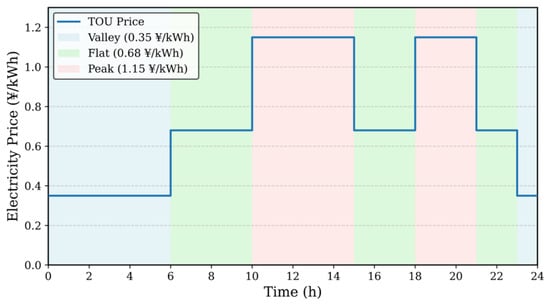
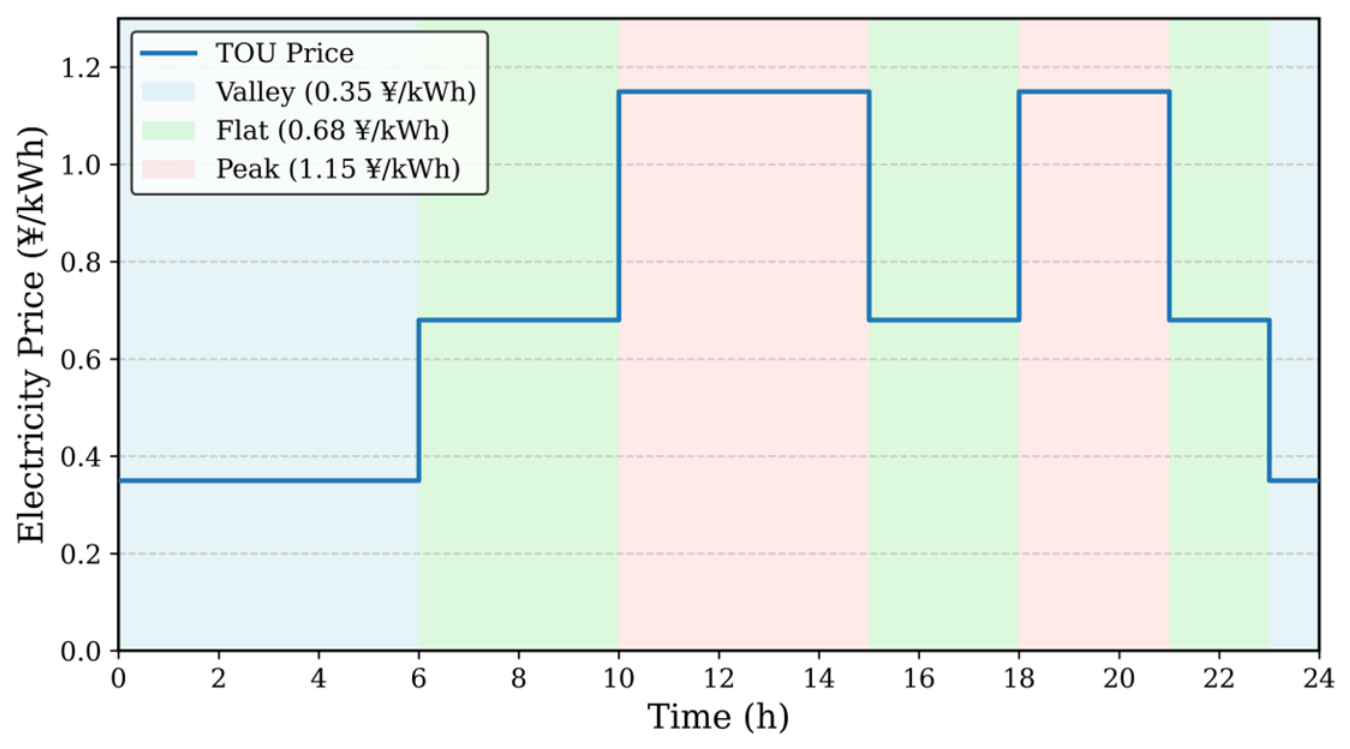
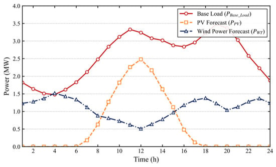
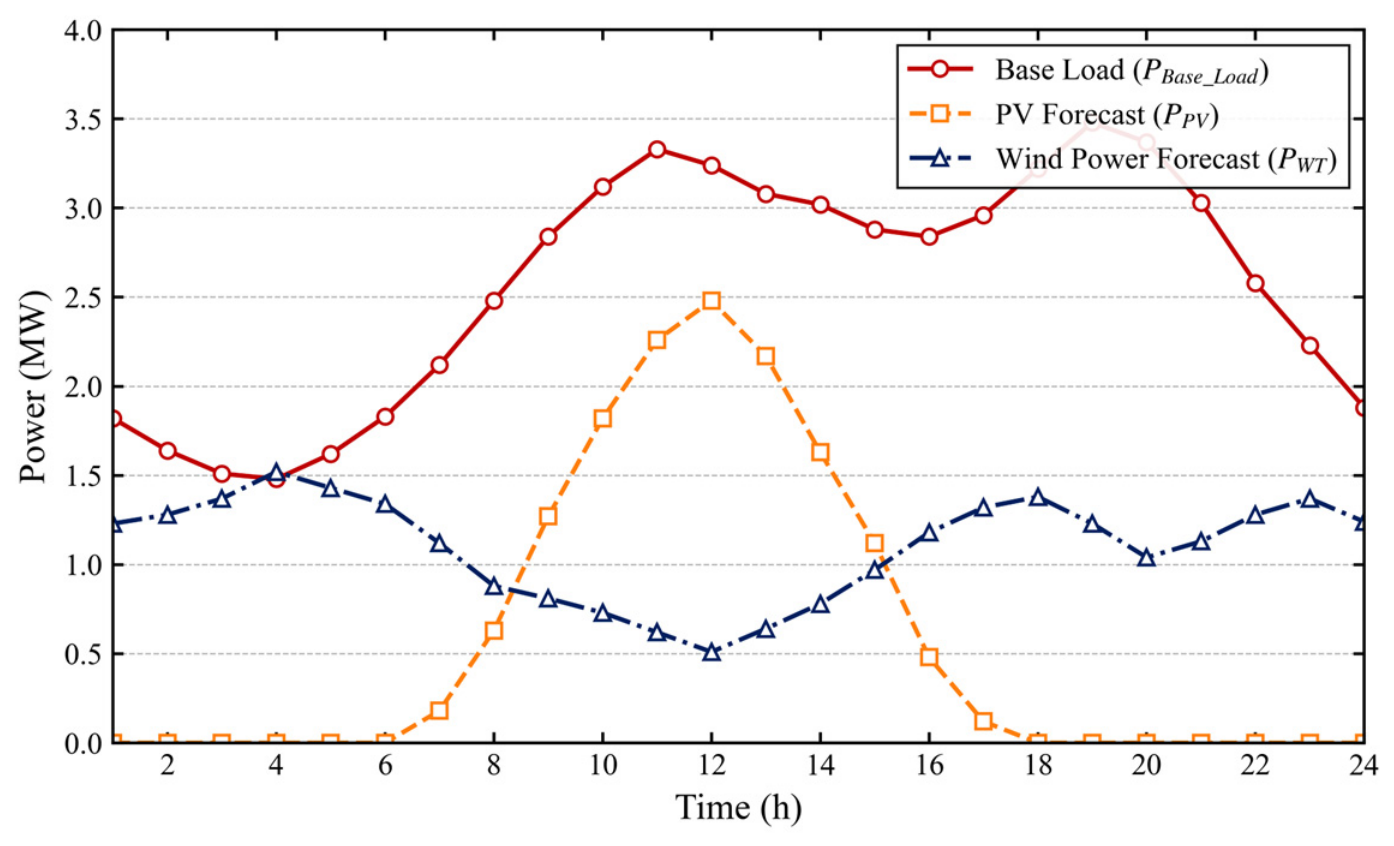
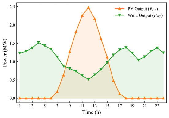
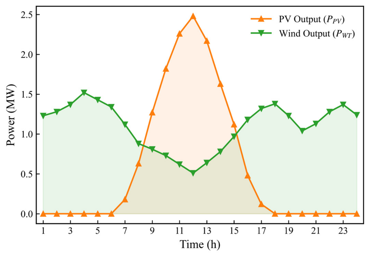
A time-of-use (TOU) electricity pricing mechanism is adopted, as depicted in Figure 5. Furthermore, the 24 h base-load demand and renewable energy generation forecasting profiles, plotted in Figure 6, serve as the unified physical input boundary conditions for all subsequent scheduling evaluations.

Figure 5. Intraday time-of-use electricity pricing profile.

Figure 6. Day-ahead forecasting profiles of base-load demand and renewable energy generation.

The commercial contract specifies a 15 min notice time, a minimum continuous call duration of 1 h, a maximum duration of 4 h, no more than four calls per day, and an active window from 09:00 to 21:00. Interruptible-load apparent-power capacities are reported in kVA. The ESS ramp limit is 0.2 p.u./min; the initial and reference SOC are both 0.50; and the charge and discharge efficiencies are 0.95. The compensation and degradation rates are 320 and 90 ¥/MWh, respectively. The ESS units at nodes 7, 11, 18, 27, and 30 use 100/215, 200/400, 100/315, 150/400, and 100/215 kW/kWh, respectively.

To systematically decouple and quantify the impacts of the proposed physical–commercial constraints and the dual-uncertainty quantification mechanisms, a progressive comparative framework comprising five models is established, as summarized in Table 4:

Model 1 (M1): Pure Physical Baseline: Constrained exclusively by the objective physical limits of the DERs. This model neglects retail price elasticity, commercial temporal constraints, and all forms of uncertainty [10].

Model 2 (M2): Unidirectional Coupling: Integrates the retail price elasticity matrix into M1 to quantify the expansion of the regulation capacity driven by economic incentives [22].

Model 3 (M3): Deterministic Dual-Coupling: Incorporates commercial contract temporal constraints (e.g., minimum continuous response duration and maximum call frequency) into M2. This serves as the core deterministic formulation of the proposed framework [18].

Model 4 (M4): Traditional Meteorological Robust: Introduces a conventional robust uncertainty set into M3, focusing solely on the objective meteorological forecasting errors associated with WT and PV generation [14].

Model 5 (M5): Proposed Comprehensive Model: Fuses the physical–commercial dual-coupling rules with the proposed dynamic robust uncertainty budget mapping mechanism derived from user credit profiles. Additionally, the high-dimensional inter-temporal constraints are decoupled utilizing the Lyapunov optimization algorithm.

Table 4. Controlled ablation study. EL: retail-price elasticity; CO: commercial temporal constraints; ME: meteorological robustness; CR: credit-driven robustness; DEC: Lyapunov temporal decoupling (M5* is the monolithic multi-period MILP of the same model). The sequence-normalized values in this table use M1 as the presentation baseline; Table 5 re-normalizes the areas with Equation (55) using M3 as the reference. The two denominators are not interchangeable.

Model	Added Component	Area Retention (rel. to M1)	Violation Prob. (95% CI)	CPU (24 h)
M1	physical baseline	1.00	21.4% [20.2%, 22.6%]	---
M2	EL	1.18	22.8% [21.6%, 24.0%]	---
M3	CO	1.09	18.65% [17.57%, 19.73%]	---
M4	ME	0.96	8.42% [7.65%, 9.19%]	---
M5	CR	0.88	2.15% [1.75%, 2.55%]	378.4 s
M5*	DEC (exact coupling)	0.88	2.15% [1.75%, 2.55%]	12,540 s

Table 4. Controlled ablation study. EL: retail-price elasticity; CO: commercial temporal constraints; ME: meteorological robustness; CR: credit-driven robustness; DEC: Lyapunov temporal decoupling (M5* is the monolithic multi-period MILP of the same model). The sequence-normalized values in this table use M1 as the presentation baseline; Table 5 re-normalizes the areas with Equation (55) using M3 as the reference. The two denominators are not interchangeable.

Model	Added Component	Area Retention (rel. to M1)	Violation Prob. (95% CI)	CPU (24 h)
M1	physical baseline	1.00	21.4% [20.2%, 22.6%]	---
M2	EL	1.18	22.8% [21.6%, 24.0%]	---
M3	CO	1.09	18.65% [17.57%, 19.73%]	---
M4	ME	0.96	8.42% [7.65%, 9.19%]	---
M5	CR	0.88	2.15% [1.75%, 2.55%]	378.4 s
M5*	DEC (exact coupling)	0.88	2.15% [1.75%, 2.55%]	12,540 s

Table 5. Reliability and geometric evaluation (third-round correction). Area retention follows Equation (55) with M3 as the reference. Every Hausdorff entry is computed against the complete M3 boundary at 20:00 with identical radial sampling and the same $n_s=96$ polyhedral mesh. The reported 20:00 active-power minima are M3 = −3.85 MW, M4 = −3.80 MW, M5 (CS = 0.92) = −3.73 MW, M5 (CS = 0.80) = −3.62 MW, and M5 (CS = 0.65) = −3.50 MW.

Model	${\mathit{P}}_{20}^{\mathbf{min}}$ (MW)	Area Retention	Violation Probability	95% CI	Hausdorff to M3 (MW)
M3	−3.85	1.00	18.65%	[17.57%, 19.73%]	0 (reference)
M4	−3.80	0.88	8.42%	[7.65%, 9.19%]	0.051
M5 (CS = 0.92)	−3.73	0.85	3.61%	[3.08%, 4.14%]	0.121
M5 (CS = 0.80)	−3.62	0.81	2.15%	[1.75%, 2.55%]	0.236
M5 (CS = 0.65)	−3.50	0.74	1.08%	[0.79%, 1.37%]	0.352

Table 5. Reliability and geometric evaluation (third-round correction). Area retention follows Equation (55) with M3 as the reference. Every Hausdorff entry is computed against the complete M3 boundary at 20:00 with identical radial sampling and the same $n_s=96$ polyhedral mesh. The reported 20:00 active-power minima are M3 = −3.85 MW, M4 = −3.80 MW, M5 (CS = 0.92) = −3.73 MW, M5 (CS = 0.80) = −3.62 MW, and M5 (CS = 0.65) = −3.50 MW.

Model	${\mathit{P}}_{20}^{\mathbf{min}}$ (MW)	Area Retention	Violation Probability	95% CI	Hausdorff to M3 (MW)
M3	−3.85	1.00	18.65%	[17.57%, 19.73%]	0 (reference)
M4	−3.80	0.88	8.42%	[7.65%, 9.19%]	0.051
M5 (CS = 0.92)	−3.73	0.85	3.61%	[3.08%, 4.14%]	0.121
M5 (CS = 0.80)	−3.62	0.81	2.15%	[1.75%, 2.55%]	0.236
M5 (CS = 0.65)	−3.50	0.74	1.08%	[0.79%, 1.37%]	0.352

5.2. Validation of the Dual-Coupled Aggregation Framework

To systematically isolate and verify the restructuring effect of the proposed physical–commercial dual-coupling mechanism, this section compares the FRs formulated by models M1, M2, and M3, operating under deterministic environments excluding uncertainty factors.

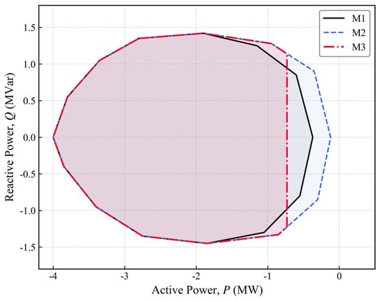
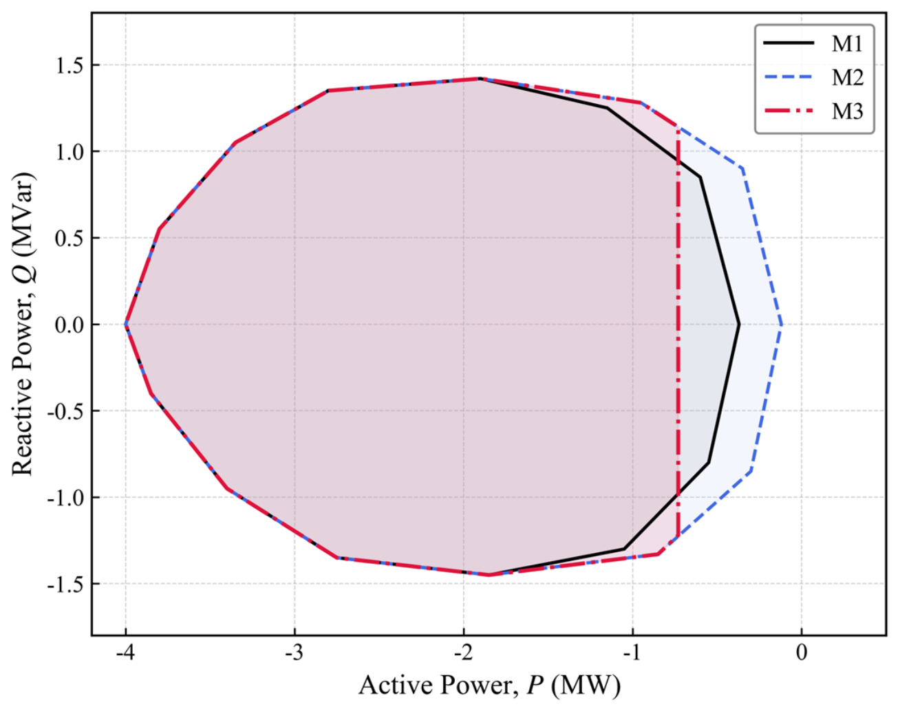
Figure 7 illustrates the cross-sectional active–reactive power FR of the VPP at the 20:00 peak-load interval. It visualizes the sequential boundary changes introduced by the retail-price mechanism and the commercial temporal constraints.

Figure 7. Cross-sectional active–reactive power FR at the 20:00 peak-load interval under the coupling models M1–M3; positive active power denotes injection; units are MW and MVar.

Relative to the physical baseline M1, the retail-price elasticity model M2 expands the active-power boundary, whereas the commercial temporal constraints in M3 contract it. Under the sign convention in Section 2.4, the M3 20:00 active-power minimum is $P_{20}^{\min }=-3.85$ MW; the guaranteed net-withdrawal magnitude is $\left|P_{20}^{\min }\right|=3.85$ MW. Figure 7 reports the projected boundary coordinates, and Table 5 reports their area retention relative to M3.

To quantify the projected areas, the theoretical area retention rate is defined as follows:

$$A_{\mathit{ret}}(\mathcal{M})={\displaystyle \frac{{\displaystyle \sum _{t=1}^T\mathit{Area}}({\mathcal{R}}_t^{\mathcal{M}})}{{\displaystyle \sum _{t=1}^T\mathit{Area}}({\mathcal{R}}_t^{\mathrm{M}3})}}$$

(55)

The numerator is the summed two-dimensional active–reactive power area of the evaluated model over the dispatch horizon, and the denominator is the corresponding area of the deterministic dual-coupled model M3.

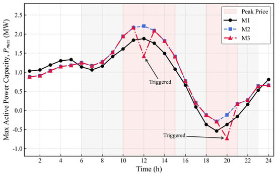
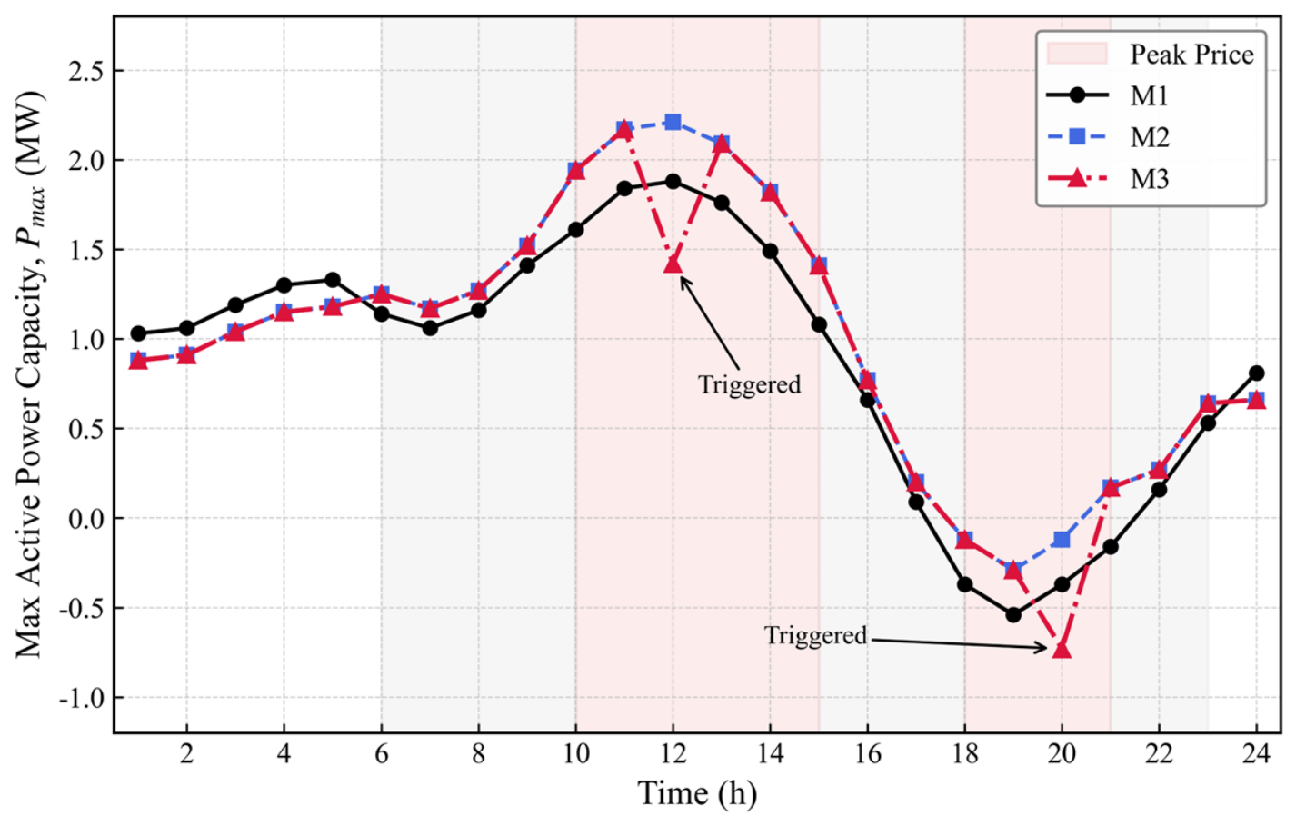
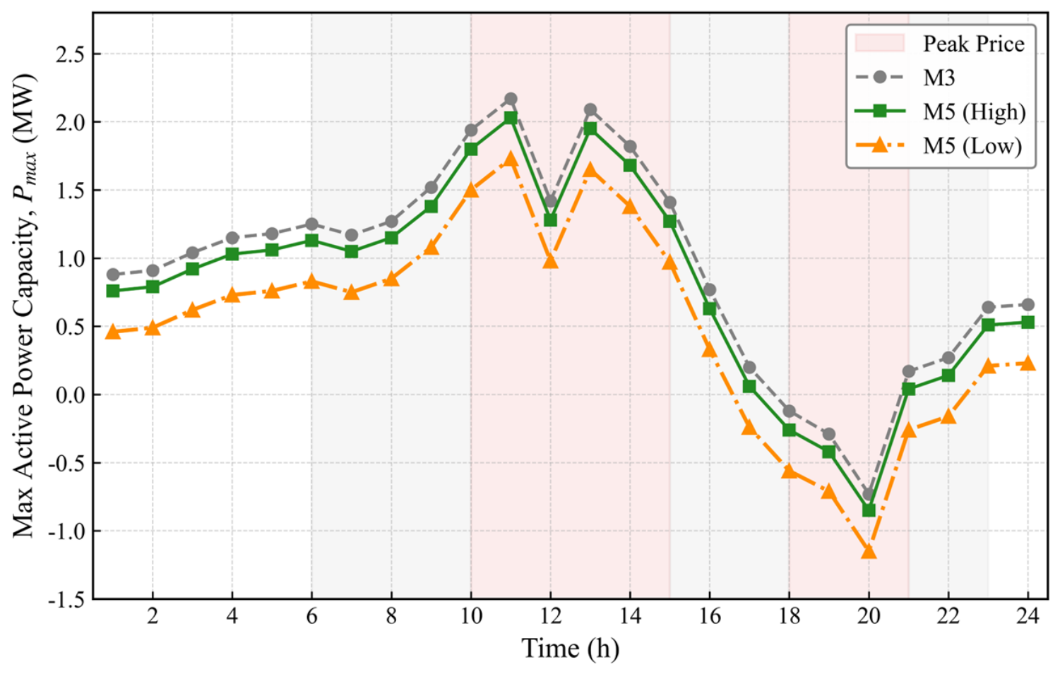
Furthermore, to evaluate the temporal evolution of these boundary limits, Figure 8 depicts the trajectory of the maximum active power regulation capacity ($P_{max}$) over the entire 24 h scheduling horizon.

Figure 8. Temporal evolution of the maximum active-power regulation capability under physical and commercial coupling (M1–M3); positive active power denotes injection; unit MW.

The trajectory analysis in Figure 8 reveals a fundamental discrepancy between purely physical estimation and practical commercial operation. While M2 exhibits a continuous, elastic capacity expansion aligned with the TOU price profile, M3 demonstrates distinct step-like capacity retractions during consecutive peak periods (e.g., at 12:00 and 20:00). These sharp declines are consistent with the inter-temporal commercial constraints preventing resource over-utilization. This phenomenon corroborates the assertion formulated in the Introduction: neglecting commercial contractual terms results in a substantial overestimation of the continuous dispatchability of the VPP.

5.3. Robustness Evaluation Under Dual Uncertainties

Having established the deterministic boundary, it is imperative to evaluate the effectiveness of the proposed dual robust budget mapping mechanism against systemic risks. This section compares the robust margins constructed under varying aggregated user credit profiles.

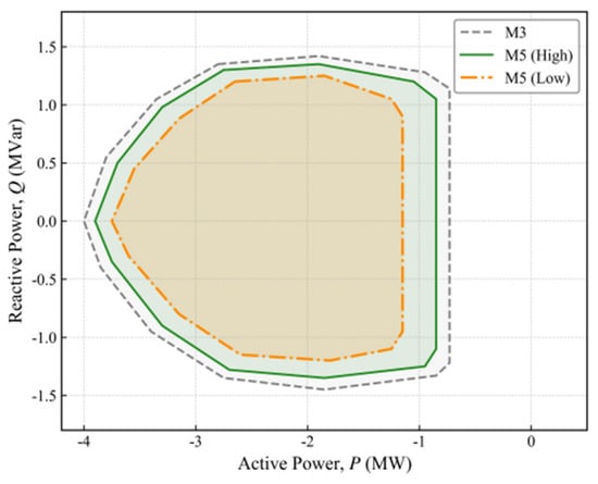
Figure 9 presents the active–reactive power FRs at 20:00 for the comprehensive model M5 under different aggregate credit levels. It illustrates how behavioral default risk is translated into engineering reserve margins.

Figure 9. Robust active–reactive power FRs at 20:00 for M3 and M5 with aggregate credit levels of 0.92, 0.80, and 0.65; positive active power denotes injection; units are MW and MVar.

Figure 9 shows an asymmetric contraction of the projected boundary. Relative to M3 with $P_{20}^{\min }=-3.85$ MW, the boundary minima are $-3.73$ MW for CS = 0.92, $-3.62$ MW for CS = 0.80, and $-3.50$ MW for CS = 0.65. Thus the guaranteed net-withdrawal magnitude decreases as credit risk increases. The smooth contraction along the reactive direction is still governed by the inverter capability.

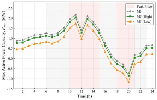
Extending this evaluation across the complete dispatch cycle, Figure 10 illustrates the temporal projection of these robust boundaries, which highlights the dynamic interaction between real-time uncertainty budgets and temporal coupling.

Figure 10. Temporal evolution of the robust active-power boundaries under dynamic credit-driven uncertainty budgets (M5); positive active power denotes injection; unit MW.

As observed in Figure 10, the reported day-ahead regulation capacity adaptively tightens in correspondence with the fluctuation of user reliability scores throughout the 24 h horizon. The feasible envelope reported to the ISO therefore exhibits robustness against sudden behavioral defaults in the tested scenarios.

To further quantify the trade-off between theoretical capability and operational reliability, Table 5 presents the results of a Monte Carlo simulation comprising 5000 randomized scenarios, which incorporate both objective meteorological forecast errors and subjective user default disturbances.

Section 5.3 uses synthetic AMI-style response records, not field measurements. The records are generated from a disclosed latent-compliance process, with 60 calibration days and 30 unseen days. The smoothing coefficient and initial score are stated below. A binary default is recorded when the regularized tracking error in Equation (27) exceeds the stated threshold. The day-block bootstrap gives ${\mathrm{\Gamma }}_{\mathit{credit}}$ intervals [1.82, 2.18], [2.76, 3.00], and [3.81, 4.00] for CS = 0.92, 0.80, and 0.65; the moment-sensitivity ranges are 3.28–3.91%, 1.91–2.44%, and 0.86–1.32%. The simulation uses 5000 scenarios with seed 20240501. The credit mechanism is therefore validated against its own synthetic generator, not against measured customer data.

The statistical metrics in Table 5 quantify the trade-off between theoretical capability and operational reliability. The deterministic model (M3) retains 100% of the theoretical area but has a dispatch violation probability of 18.65% (95% CI [17.57%, 19.73%]). The traditional meteorological robust model (M4) reduces the violation risk to 8.42% (95% CI [7.65%, 9.19%]). By quantifying both dimensions of uncertainty, M5 reduces the dispatch violation probability to 2.15% (95% CI [1.75%, 2.55%]) at an area retention rate of 0.81.

5.4. Computational Efficiency of the Inter-Temporal Decoupling Algorithm

The incorporation of ESS SOC dynamics and commercial duration limits inherently transforms the FR characterization into a high-dimensional inter-temporal optimization problem. Table 6 evaluates the computational performance of the proposed Lyapunov-based decoupling algorithm against the monolithic multi-period MILP (M5*) solved with CPLEX 22.1, a MIP gap of 1 × 10⁻⁴, and a warm start.

Table 6. CPU time (s) for horizons of 1, 4, 8, 12, and 24 h on the 33-, 69-, and 123-node feeders (CPLEX 22.1, MIP gap 1 × 10⁻⁴, warm start). M5* denotes the monolithic multi-period MILP of the same model.

Horizon (h)	1	4	8	12	24
M5*, 33-node	14.5	78.2	412.5	1845.6	12,540
M5, 33-node	15.2	62.4	125.8	186.5	378.4
M5, 69-node	27.4	118.7	241.2	358.9	692.3
M5, 123-node	44.6	198.3	402.6	601.4	1147.2

The timing analysis in Table 6 shows 12,540 s for the 24 h monolithic M5* model and 378.4 s for the decoupled M5 implementation. The OPA verification uses $n_s=96$ and $n_s=192$ for the mesh comparison. The distance between the decoupled and monolithic versions of the same M5 model is 0.008 MW, with a 0.9% projected-area difference. The trends are empirical and limited to the tested horizons and feeders.

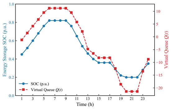
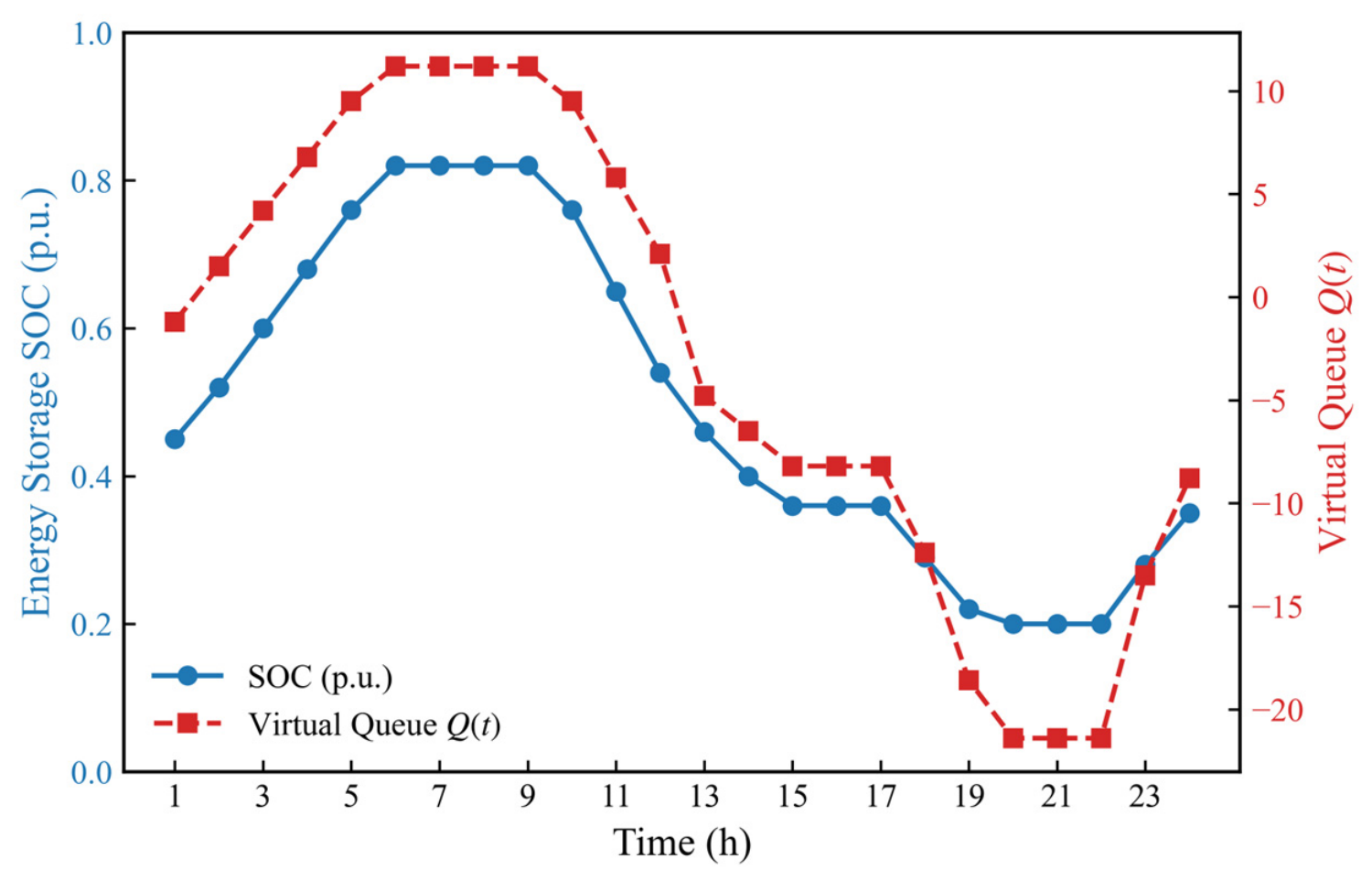
To assess whether the slot-wise DPP construction preserves the inter-temporal behavior, Figure 11 tracks a representative ESS SOC trajectory and the Lyapunov virtual queue. The figure does not assert exact finite-horizon terminal recovery.

Figure 11. Dynamic trajectories of the Lyapunov virtual queue and the energy storage SOC over a 24 h horizon (M5; SOC in p.u. and virtual queue in queue units).

The terminal equality ${\mathit{SOC}}_{i,T}={\mathit{SOC}}_{i,0}$ is not imposed as a hard constraint of every slot-wise subproblem. The DPP policy provides asymptotic queue stability, not finite-horizon terminal feasibility. The representative trajectory in Figure 11 ends near 0.35 p.u.; starting from the 0.50 p.u. reference, its terminal deviation is approximately 0.15 p.u. Exact terminal recovery would require a separate terminal-stage MILP.

5.5. VPP Coordinated Dispatch and Comprehensive Economic Assessment

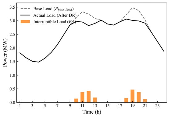
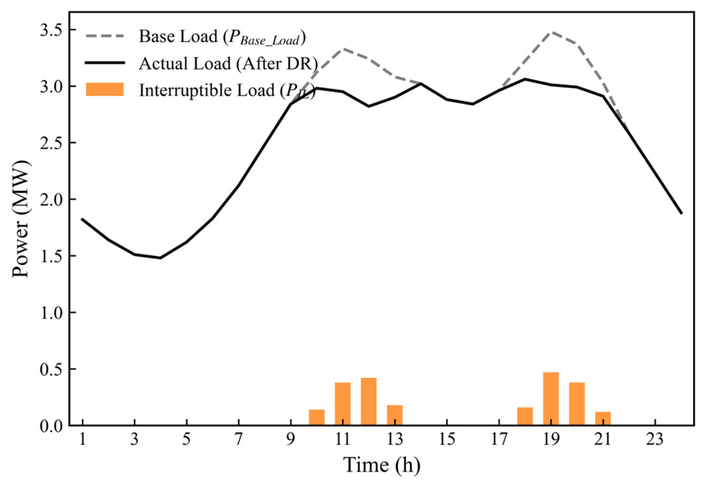
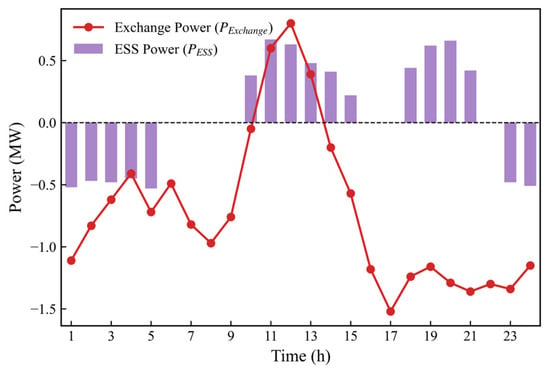
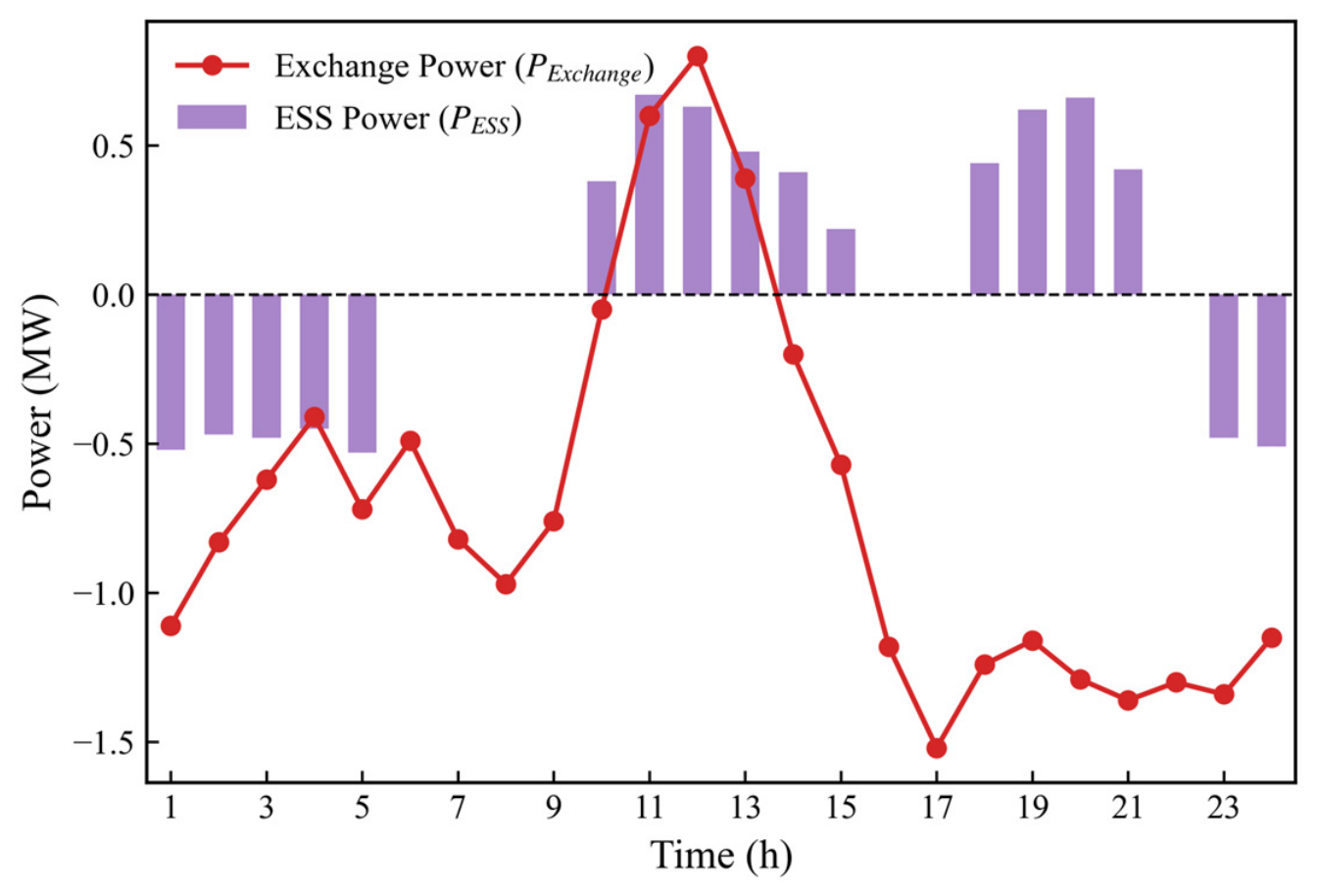
To complete the closed-loop validation, the physical reliability of the proposed FR is evaluated through a standard day-ahead coordinated-dispatch case. Figure 12, Figure 13 and Figure 14 show the optimal dispatch of loads, renewable generation, ESS units, and PCC exchange power. Positive PCC active power denotes injection and negative PCC active power denotes withdrawal.

Figure 12. Base load and responsive interruptible load dispatch trajectories under the optimal strategy (M5; unit MW).

Figure 13. Distributed renewable energy (photovoltaic and wind) output scheduling trajectories (M5; unit MW).

Figure 14. ESS operating power and PCC exchange-power trajectories (M5); positive active power denotes injection; unit MW.

The 20:00 robust-boundary check and the dispatch trajectory refer to different objects. For M5 with CS = 0.80, the active-power boundary minimum is $P_{20}^{\min }=-3.62$ MW. The feasibility check returns zero violation at −3.62 MW and a positive violation at −3.63 MW. Figure 14 is a dispatch trajectory; its 20:00 PCC power is approximately −1.30 MW and lies inside the robust boundary. Under the convention $P>0$ for injection and $P<0$ for withdrawal, the boundary wording is expressed through $P_{20}^{\min }$ and the withdrawal magnitude $\left|P_{20}^{\min }\right|$, not through an ambiguous upper limit.

Finally, Table 7 summarizes the comprehensive system-level economic settlement parameters across the full scheduling cycle to evaluate the financial viability of the formulated models.

Table 7. System-level economic settlement (revised). Settlement follows Equations (56)–(59); the penalty, compensation, and degradation prices are 1200, 320, and 90 yuan/MWh, respectively.

Assessment Metric	M3	M4	M5
Market arbitrage revenue (¥)	35,420	32,150	−12,378
Internal compensation and degradation (¥)	3970	3730	3400
Default energy (MWh)	5.80	4.88	0.38
Default penalty (¥)	6960	5856	456
Net profit (¥)	24,490	22,564	−16,234

The day-ahead settlement is defined by the following accounting identities. Positive $P_{\mathit{pcc}}$ contributes market revenue and negative $P_{\mathit{pcc}}$ contributes market cost under the stated sign convention.

$$R^{\mathit{arb}}={\displaystyle \sum _{t=1}^T{\lambda }_t}{P}_{\mathit{pcc}}(t)\Delta t$$

(56)

The internal compensation and degradation cost is as follows:

$$C^{\mathit{int}}={\displaystyle \sum _{j,t}{c}^{\mathit{comp}}}|P_j(t)|\Delta t+{\displaystyle \sum _{s,t}{c}^{\mathit{deg}}}[P_s^{\mathit{ch}}(t)+P_s^{\mathit{dis}}(t)]\Delta t$$

(57)

The default penalty is as follows:

$${\mathrm{\Pi }}^{\mathit{pen}}=p^{\mathit{pen}}{\displaystyle \sum _{j,t}\max }\{0,P_j^{*}(t)-P_j^{\mathit{act}}(t)\}\Delta t$$

(58)

The net profit is as follows:

$${\mathrm{\Pi }}^{\mathit{net}}=R^{\mathit{arb}}-C^{\mathit{int}}-{\mathrm{\Pi }}^{\mathit{pen}}$$

(59)

The compensation, degradation, and default-penalty prices are 320, 90, and 1200 ¥/MWh. The default-eligible set contains only the four ILs at nodes 8, 22, 24, and 28 and the active window is 09:00–21:00. The default energy is $E_{\mathit{def}}={\displaystyle \frac{1}{N_{\mathit{MC}}}}{\displaystyle \sum _{m=1}^{N_{\mathit{MC}}}{\displaystyle \sum _{t=9}^{21}{\displaystyle \sum _{j\in \{8,22,24,28\}}\left|\Delta P_{j,m}(t)\right|}}}\Delta t$. The IL-only upper bound is $610 \mathrm{kVA}\times 0.9\times 12 \mathrm{h}=6.588$ MWh. The recomputed default energies are 5.80 MWh for M3, 4.88 MWh for M4, and 0.38 MWh for M5. RES and ESS units are not default-eligible and receive no behavioral-default penalty. A quantitative comparison with the closest time-domain coupling methods is summarized in Table 8. The sensitivity of the net profit to the default-penalty price is reported in Table 9.

Table 8. Quantitative comparison with time-domain coupling methods (modified 33-node system, 24 h, same dispatch scenario). The reported 0.008 MW is the Hausdorff distance between the decoupled M5 boundary and the monolithic M5* boundary of the same model; it is not a distance to M3.

Method	Area Retention	Hausdorff (MW)	CPU Time (s)
Proposed M5	0.81	0.008	378
Ref. [17]	0.79	0.012	2410
Ref. [18]	0.78	0.015	5620
Ref. [19]	0.80	0.011	1860

Table 8. Quantitative comparison with time-domain coupling methods (modified 33-node system, 24 h, same dispatch scenario). The reported 0.008 MW is the Hausdorff distance between the decoupled M5 boundary and the monolithic M5* boundary of the same model; it is not a distance to M3.

Method	Area Retention	Hausdorff (MW)	CPU Time (s)
Proposed M5	0.81	0.008	378
Ref. [17]	0.79	0.012	2410
Ref. [18]	0.78	0.015	5620
Ref. [19]	0.80	0.011	1860

Table 9. Sensitivity of net profit to the default-penalty price. The M3 default energy is 5.80 MWh and the M5 market-arbitrage revenue is −12,378 ¥. The M5 net profit is negative at every penalty price shown. The M3/M4 crossover occurs at approximately 3294 ¥/MWh; the M3/M5 and M4/M5 crossovers lie above 3000 ¥/MWh.

${\mathit{p}}_{\mathit{pen}}$ (¥/MWh)	0	216	325	388	1200	3000
M3	31,450	30,197	29,565	29,200	24,490	14,050
M4	28,420	27,366	26,834	26,527	22,564	13,780
M5	−15,778	−15,860	−15,902	−15,925	−16,234	−16,918

Table 9. Sensitivity of net profit to the default-penalty price. The M3 default energy is 5.80 MWh and the M5 market-arbitrage revenue is −12,378 ¥. The M5 net profit is negative at every penalty price shown. The M3/M4 crossover occurs at approximately 3294 ¥/MWh; the M3/M5 and M4/M5 crossovers lie above 3000 ¥/MWh.

${\mathit{p}}_{\mathit{pen}}$ (¥/MWh)	0	216	325	388	1200	3000
M3	31,450	30,197	29,565	29,200	24,490	14,050
M4	28,420	27,366	26,834	26,527	22,564	13,780
M5	−15,778	−15,860	−15,902	−15,925	−16,234	−16,918

The complete hourly audit is reported in Table 10. It lists $P_{\mathit{PCC}}(t)$, $\pi (t)$, the signed contribution $P_{\mathit{PCC}}(t)\pi (t)\Delta t$, and the cumulative sum. The sum is $-\mathrm{12,377.5}$ ¥, which rounds to $-\mathrm{12,378}$ ¥. The identity $\mathrm{30,850}=\mathrm{27,450}+3400$ is not an independent external check and has been removed.

The economic results are conditional on the disclosed prices, the synthetic default energy, and the dispatch trajectory. Under the sign convention $P>0$ for injection and $P<0$ for withdrawal, the M5 hourly arbitrage revenue is $-\mathrm{12,378}$ ¥, the internal compensation and degradation cost is 3400 ¥, and the default penalty at 1200 ¥/MWh is $0.38\times 1200=456$ ¥. The M5 net profit is therefore $-\mathrm{12,378}-3400-456=-\mathrm{16,234}$ ¥. These results do not establish an economic advantage for M5 over M3 or M4 for this dispatch.

Table 10. Hourly market-settlement audit for the M5 dispatch trajectory shown in Figure 14. The sign convention is $P_{\mathit{PCC}}>0$ for injection and $P_{\mathit{PCC}}<0$ for withdrawal. Contributions use $\Delta t=1$ h and sum to −12,377.5 ¥.

Hour	PPCC (MW)	π (¥/MWh)	Signed Contribution (¥)	Cumulative (¥)
1	−1.1	0.35	−0.4	−0.4
2	−0.75	0.35	−0.3	−0.6
3	−0.42	0.35	−0.1	−0.8
4	−0.65	0.35	−0.2	−1.0
5	−0.8	0.35	−0.3	−1.3
6	−1.3	0.35	−0.5	−1.8
7	−0.75	0.68	−0.5	−2.3
8	−0.6	0.68	−0.4	−2.7
9	−1.1	0.68	−0.7	−3.4
10	0.95	0.68	0.6	−2.8
11	0.65	1.15	0.7	−2.0
12	0.3	1.15	0.3	−1.7
13	−0.1	1.15	−0.1	−1.8
14	−0.45	1.15	−0.5	−2.3
15	−1.2	1.15	−1.4	−3.7
16	−1.4	0.68	−1.0	−4.6
17	−1.15	0.68	−0.8	−5.4
18	−1.05	0.68	−0.7	−6.1
19	−1.2	1.15	−1.4	−7.5
20	−1.3	1.15	−1.5	−9.0
21	−1.3	1.15	−1.5	−10.5
22	−1.1	0.68	−0.7	−11.3
23	−1.15	0.68	−0.8	−12.0
24	−0.95	0.35	−0.3	−12.4

Table 10. Hourly market-settlement audit for the M5 dispatch trajectory shown in Figure 14. The sign convention is $P_{\mathit{PCC}}>0$ for injection and $P_{\mathit{PCC}}<0$ for withdrawal. Contributions use $\Delta t=1$ h and sum to −12,377.5 ¥.

Hour	PPCC (MW)	π (¥/MWh)	Signed Contribution (¥)	Cumulative (¥)
1	−1.1	0.35	−0.4	−0.4
2	−0.75	0.35	−0.3	−0.6
3	−0.42	0.35	−0.1	−0.8
4	−0.65	0.35	−0.2	−1.0
5	−0.8	0.35	−0.3	−1.3
6	−1.3	0.35	−0.5	−1.8
7	−0.75	0.68	−0.5	−2.3
8	−0.6	0.68	−0.4	−2.7
9	−1.1	0.68	−0.7	−3.4
10	0.95	0.68	0.6	−2.8
11	0.65	1.15	0.7	−2.0
12	0.3	1.15	0.3	−1.7
13	−0.1	1.15	−0.1	−1.8
14	−0.45	1.15	−0.5	−2.3
15	−1.2	1.15	−1.4	−3.7
16	−1.4	0.68	−1.0	−4.6
17	−1.15	0.68	−0.8	−5.4
18	−1.05	0.68	−0.7	−6.1
19	−1.2	1.15	−1.4	−7.5
20	−1.3	1.15	−1.5	−9.0
21	−1.3	1.15	−1.5	−10.5
22	−1.1	0.68	−0.7	−11.3
23	−1.15	0.68	−0.8	−12.0
24	−0.95	0.35	−0.3	−12.4

6. Conclusions

This paper presents a multi-dimensional robust FR characterization framework for VPPs considering commercial constraints and inter-temporal decoupling. The framework was validated on a modified 33-node active distribution network, with additional scaling tests on 69- and 123-node feeders. The main conclusions are summarized as follows:

(i) In the tested system, commercial clauses contract the elasticity-expanded M2 envelope by about 7.6% under the sequence-normalized areas in Table 4. The Table 4 baseline M1 and the M3-normalized areas in Table 5 are reported separately, because mixing the two denominators caused the previous wording to overstate the reduction.

(ii) Under the specified uncertainty model and out-of-sample simulation protocol, the credit-driven budget reduces the estimated dispatch-violation probability from 18.65% to 2.15%. The confidence interval and the one-sided correlation bound should be interpreted together with the modeling assumptions.

(iii) For the tested feeders, epigraph-based dimensionality reduction and Lyapunov temporal decoupling reduce the reported CPU time from 12,540 s to 378 s. The Hausdorff distance between the decoupled and monolithic versions of the same M5 model is 0.008 MW. This value is distinct from the M3-to-M5 contraction distances in Table 5. The results are simulation-based and do not provide a general optimality or real-time performance guarantee.

References

- Abdelkader, S.; Amissah, J.; Abdel-Rahim, O. Virtual Power Plants: An in-Depth Analysis of Their Advancements and Importance as Crucial Players in Modern Power Systems. Energy Sustain. Soc. 2024, 14, 52. [Google Scholar] [CrossRef] [Scilit]
- Alam, M.S.; Al-Ismail, F.S.; Salem, A.; Abido, M.A. High-Level Penetration of Renewable Energy Sources into Grid Utility: Challenges and Solutions. IEEE Access 2020, 8, 190277–190299. [Google Scholar] [CrossRef] [Scilit]
- Kaiss, M.; Wan, Y.; Gebbran, D.; Vila, C.U.; Dragičević, T. Review on Virtual Power Plants/Virtual Aggregators: Concepts, Applications, Prospects and Operation Strategies. Renew. Sustain. Energy Rev. 2025, 211, 115242. [Google Scholar] [CrossRef] [Scilit]
- Koch, S.; Andersson, G. Assessment of Revenue Potentials of Ancillary Service Provision by Flexible Unit Portfolios. In Proceedings of the 2012 IEEE Power and Energy Society General Meeting; IEEE: Piscataway, NJ, USA, 2012; pp. 1–8. [Google Scholar]
- Abbasi, M.H.; Taki, M.; Rajabi, A.; Li, L.; Zhang, J. Coordinated Operation of Electric Vehicle Charging and Wind Power Generation as a Virtual Power Plant: A Multi-Stage Risk Constrained Approach. Appl. Energy 2019, 239, 1294–1307. [Google Scholar] [CrossRef] [Scilit]
- Ju, L.; Li, H.; Zhao, J.; Chen, K.; Tan, Q.; Tan, Z. Multi-Objective Stochastic Scheduling Optimization Model for Connecting a Virtual Power Plant to Wind-Photovoltaic-Electric Vehicles Considering Uncertainties and Demand Response. Energy Convers. Manag. 2016, 128, 160–177. [Google Scholar] [CrossRef] [Scilit]
- Silva, J.; Sumaili, J.; Bessa, R.J.; Seca, L.; Matos, M.A.; Miranda, V.; Caujolle, M.; Goncer, B.; Sebastian-Viana, M. Estimating the Active and Reactive Power Flexibility Area at the TSO-DSO Interface. IEEE Trans. Power Syst. 2018, 33, 4741–4750. [Google Scholar] [CrossRef] [Scilit]
- Zhao, L.; Zhang, W.; Hao, H.; Kalsi, K. A Geometric Approach to Aggregate Flexibility Modeling of Thermostatically Controlled Loads. IEEE Trans. Power Syst. 2017, 32, 4721–4731. [Google Scholar] [CrossRef] [Scilit]
- Müller, F.L.; Sundström, O.; Szabó, J.; Lygeros, J. Aggregation of Energetic Flexibility Using Zonotopes. In Proceedings of the 2015 54th IEEE Conference on Decision and Control (CDC); IEEE: Piscataway, NJ, USA, 2015; pp. 6564–6569. [Google Scholar]
- Wen, Y.; Hu, Z.; You, S.; Duan, X. Aggregate Feasible Region of DERs: Exact Formulation and Approximate Models. IEEE Trans. Smart Grid 2022, 13, 4405–4423. [Google Scholar] [CrossRef] [Scilit]
- Wang, Y.; Zhong, H.; Ruan, G. A Projection-Based Approach for Distributed Energy Resources Aggregation. In Proceedings of the 2023 IEEE PES Innovative Smart Grid Technologies Europe (ISGT EUROPE); IEEE: Piscataway, NJ, USA, 2023; pp. 1–5. [Google Scholar]
- Riaz, S.; Mancarella, P. Modelling and Characterisation of Flexibility from Distributed Energy Resources. IEEE Trans. Power Syst. 2022, 37, 38–50. [Google Scholar] [CrossRef] [Scilit]
- Tan, Z.; Zhong, H.; Xia, Q.; Kang, C.; Wang, X.S.; Tang, H. Estimating the Robust PQ Capability of a Technical Virtual Power Plant under Uncertainties. IEEE Trans. Power Syst. 2020, 35, 4285–4296. [Google Scholar] [CrossRef] [Scilit]
- Lubin, M.; Dvorkin, Y.; Backhaus, S. A Robust Approach to Chance Constrained Optimal Power Flow with Renewable Generation. IEEE Trans. Power Syst. 2016, 31, 3840–3849. [Google Scholar] [CrossRef] [Scilit]
- Yang, X.; Li, Y.; Zhao, Y.; Li, Y.; Hao, G.; Wang, Y. Gaussian Mixture Model Uncertainty Modeling for Power Systems Considering Mutual Assistance of Latent Variables. IEEE Trans. Sustain. Energy 2024, 15, 1694–1708. [Google Scholar] [CrossRef] [Scilit]
- Wang, H.; Jia, Y.; Lai, C.S.; Li, K. Optimal Virtual Power Plant Operational Regime under Reserve Uncertainty. IEEE Trans. Smart Grid 2022, 13, 2973–2985. [Google Scholar] [CrossRef] [Scilit]
- Wang, S.; Wu, W. Aggregate Flexibility of Virtual Power Plants with Temporal Coupling Constraints. IEEE Trans. Smart Grid 2021, 12, 5043–5051. [Google Scholar] [CrossRef] [Scilit]
- Zhang, T.; Wang, J.; Li, G.; Wang, X.; Zhou, M. Characterizing Temporal-Coupled Feasible Region of Active Distribution Networks. IEEE Trans. Ind. Appl. 2022, 58, 5687–5696. [Google Scholar] [CrossRef] [Scilit]
- Xu, Z.; He, J.; Liu, Z.; Chen, W.; Wang, X.; Zhang, P. Solution Method of Virtual Power Plant Dynamic Feasible Region Based on Decoupling of Coupling Constraints. Proc. CSEE 2024, 44, 3440–3452. [Google Scholar]
- Pourghaderi, N.; Fotuhi-Firuzabad, M.; Moeini-Aghtaie, M.; Kabirifar, M.; Lehtonen, M. Exploiting DERs’ Flexibility Provision in Distribution and Transmission Systems Interface. IEEE Trans. Power Syst. 2023, 38, 1963–1977. [Google Scholar] [CrossRef] [Scilit]
- Yi, Z.; Xu, Y.; Gu, W.; Yang, L.; Sun, H. Aggregate Operation Model for Numerous Small-Capacity Distributed Energy Resources Considering Uncertainty. IEEE Trans. Smart Grid 2021, 12, 4208–4224. [Google Scholar] [CrossRef] [Scilit]
- Hamidi, A.; Hamzeh, M.; Bozorg, M.; Cherkaoui, R. Performance-Based Capacity Allocation of DERs to Improve Aggregated Flexibility Provision. IEEE Trans. Smart Grid 2025, 16, 2968–2990. [Google Scholar] [CrossRef] [Scilit]
- Liu, X.; Li, Y.; Wang, L.; Tang, J.; Qiu, H.; Berizzi, A.; Valentin, I.; Gao, C. Dynamic Aggregation Strategy for a Virtual Power Plant to Improve Flexible Regulation Ability. Energy 2024, 297, 131261. [Google Scholar] [CrossRef] [Scilit]
- Müller, F.L.; Szabó, J.; Sundström, O.; Lygeros, J. Aggregation and Disaggregation of Energetic Flexibility from Distributed Energy Resources. IEEE Trans. Smart Grid 2019, 10, 1205–1214. [Google Scholar] [CrossRef] [Scilit]
- Wu, C.; Gu, W.; Zhou, S.; Chen, X. Coordinated Optimal Power Flow for Integrated Active Distribution Network and Virtual Power Plants Using Decentralized Algorithm. IEEE Trans. Power Syst. 2021, 36, 3541–3551. [Google Scholar] [CrossRef] [Scilit]
- Girigoudar, K.; Roald, L.A. Identifying Secure Operating Ranges for DER Control Using Bilevel Optimization. IEEE Trans. Smart Grid 2023, 15, 2921–2933. [Google Scholar] [CrossRef] [Scilit]
- Chiang, H.-D.; Jiang, C.-Y. Feasible Region of Optimal Power Flow: Characterization and Applications. IEEE Trans. Power Syst. 2018, 33, 236–244. [Google Scholar] [CrossRef] [Scilit]
- Ju, Y.; Chen, C.; Wu, L.; Liu, H. General Three-Phase Linear Power Flow for Active Distribution Networks with Good Adaptability under a Polar Coordinate System. IEEE Access 2018, 6, 34043–34050. [Google Scholar] [CrossRef] [Scilit]
Disclaimer/Publisher’s Note: The statements, opinions and data contained in all publications are solely those of the individual author(s) and contributor(s) and not of MDPI and/or the editor(s). MDPI and/or the editor(s) disclaim responsibility for any injury to people or property resulting from any ideas, methods, instructions or products referred to in the content. |
© 2026 by the authors. Licensee MDPI, Basel, Switzerland. This article is an open access article distributed under the terms and conditions of the Creative Commons Attribution (CC BY) license.