


Abstract
The increasing penetration of converter-interfaced renewable generation and the declining share of synchronous generation reduce voltage and frequency support. This paper proposes a grid-forming (GFM) converter capacity ratio estimation method and a capability assessment framework for hybrid grid-following (GFL) and GFM converter systems at fixed total installed capacity. First, a model incorporating the principal control loops of both converter types is developed. The critical short-circuit ratio and the GFM converter terminal impedance are used to derive an analytical relationship between the GFM capacity ratio and the generalized short-circuit ratio. This relationship defines a continuous lower bound for the capacity ratio subject to small-signal stability and target grid strength constraints. The assessment framework uses normalized margins and a bottleneck index to evaluate basic support conditions, control parameter effects, and disturbance response performance. Generalized Nyquist analysis and time-domain simulations verify the method. Under the studied conditions, increasing the GFM capacity ratio increases equivalent grid strength and oscillation damping, reduces the peak power deviation, and shortens the settling time. Phase-locked loop parameters mainly affect synchronization dynamics and power oscillations, whereas virtual inertia and the damping coefficient primarily affect frequency support and power recovery. The method supports GFM capacity planning and control coordination.
1. Introduction
With the increasing integration of wind and photovoltaic generation, the share of conventional synchronous generation is declining, whereas the share of converter-interfaced generation continues to increase. Consequently, power systems are shifting from synchronous generation toward operation dominated by converters [1]. Power electronic converters serve as grid interfaces for renewable generation. They generally use either grid-following (GFL) or grid-forming (GFM) control. GFL converters typically use current control to inject power. They employ a phase-locked loop (PLL) to track the voltage phase and frequency at the point of connection. Their stable operation therefore relies on the external grid for voltage and frequency references [2,3]. Under weak grid conditions, high grid impedance strengthens the coupling between the converter, the grid, and its control loops. This coupling reduces the synchronization stability margin and may also cause power oscillations or transient loss of synchronism [4,5]. GFM converters autonomously establish grid voltage and frequency while providing active grid support through virtual inertia, damping, and voltage regulation. Owing to their voltage source characteristics, they are suited to weak grid and islanded operation, thereby offering an important technical solution for enhancing the stability and effective grid strength of power systems with high renewable energy penetration [6,7].
However, renewable energy plants face high retrofit costs, different control functions, and varying operating requirements. GFL and GFM converters are therefore expected to coexist for the foreseeable future. The GFM converter capacity ratio affects both the equivalent grid strength and the small-signal stability margin of the hybrid system. If this ratio is insufficient, GFM converters may provide inadequate voltage support to improve the synchronization stability and oscillation damping of GFL converters [8]. A higher GFM capacity ratio generally improves grid strength but may also increase investment costs [9]. The capacity ratio alone cannot fully characterize the grid-forming capability of a plant because support performance also depends on external grid strength, control parameters, and operating conditions. A key task in renewable energy plant planning is to determine the minimum GFM capacity ratio that satisfies the small-signal stability and target grid strength requirements. The grid-forming capability of the resulting hybrid system must also be assessed to support coordinated control design.
The existing studies on the GFM converter capacity ratio in hybrid systems have primarily addressed grid strength and small-signal stability. The generalized short-circuit ratio (gSCR) and critical short-circuit ratio (CSCR) link grid strength to the small-signal stability boundary of converters [10], while appropriate placement of GFM converters can increase the equivalent grid strength and improve the stability margin of PLL-based converters [11]. Furthermore, the study in [12] characterized the effective voltage source behavior of GFM converters from a dynamic admittance perspective and established an analytical relationship among the GFM capacity ratio, gSCR, and a specified stability margin by representing each GFM converter as an ideal voltage source behind an equivalent scalar reactance. The study in [13] determined feasible GFM capacity ranges for different GFM configurations by jointly considering gSCR, the equipment CSCR, and steady-state operating constraints. These studies provide a theoretical basis for estimating GFM capacity ratio. The equivalent reactance in [12] is obtained from the GFM impedance characteristic at a frequency of interest, whereas the capacity boundary in [13] depends on prescribed stability margins and steady-state operating constraints. For a renewable energy plant with a fixed total installed capacity, in which GFM units replace part of the existing GFL capacity, the required GFM capacity ratio should therefore be determined by accounting for the actual control parameters and frequency-dependent terminal characteristics of the GFM converters.
On the other hand, satisfying a target gSCR or small-signal stability margin does not fully characterize the actual grid-forming capability of a hybrid system during disturbances. Previous studies have shown that the GFM stability boundary is affected by inner loop parameters, network conditions, and operating points [14], and that interactions between heterogeneous GFL and GFM controls alter the oscillatory characteristics of hybrid systems [15]. Accordingly, research at the system level has expanded from gSCR assessment to control admittance and modular impedance analysis [16,17,18]. Although these studies deepen the understanding of the relationship between the GFM converter capacity ratio and small-signal stability, they still focus primarily on local stability. Related research has therefore expanded from stability boundaries to disturbance response performance. Regarding frequency response, ref. [19] analyzed the frequency nadir and rate of change of frequency (RoCoF) for different GFM capacity ratios. For dynamics induced by faults, ref. [20] investigated the effects of grid strength, virtual inertia, and damping on transient synchronization. The analysis in [21] further showed that the preferred GFM converter capacity ratio differs between load disturbances and single-phase-to-ground faults. It also found that a configuration consisting entirely of GFM converters may not provide optimal voltage and frequency support under fault conditions. Thus, a capacity ratio that satisfies small-signal stability requirements does not necessarily yield optimal grid-forming support during disturbances.
Overall, most existing methods address a single stability issue or a specific disturbance. However, a clear link between preliminary estimation of the GFM capacity ratio and multidimensional dynamic assessment remains lacking. Consequently, determining an appropriate GFM capacity ratio subject to a fixed total installed capacity remains an important problem in renewable energy plant planning and control design. This task also involves a comprehensive assessment of the hybrid system under different control parameters and representative disturbances. Such an assessment encompasses equivalent grid strength, oscillation damping, frequency support, and dynamic recovery.
To address these issues, this paper considers a single-infeed hybrid wind farm comprising GFL and GFM converters with a fixed total installed capacity. A hybrid system model incorporating the principal control loops of both converter types is first established. The model is then used to determine the minimum GFM capacity ratio required to satisfy small-signal stability and target grid strength requirements. On this basis, a grid-forming capability assessment framework is developed. The framework evaluates four categories of factors, namely, system strength, the GFM converter capacity ratio, control parameters, and small-disturbance response performance. These factors are organized into three assessment levels to comprehensively characterize the grid-forming capability of the hybrid system. Finally, frequency-domain analysis and time-domain simulations validate the proposed GFM converter capacity ratio estimation method and assessment framework.
The main contributions of this paper are summarized as follows:
- (1)
- A preliminary GFM converter capacity ratio estimation method is proposed under a fixed total installed capacity. For a configuration in which GFM capacity replaces part of the existing GFL capacity, the external grid strength, the critical stability boundary of the GFL converter, and the dynamic terminal support of the GFM converter are incorporated into a unified calculation. An analytical relationship between the GFM capacity ratio and the gSCR is derived to obtain continuous lower bounds that satisfy the small-signal stability boundary and the target grid strength requirement, respectively. Frequency-domain stability is then verified using the generalized Nyquist criterion.
- (2)
- A multidimensional grid-forming capability assessment framework is developed for the hybrid system. The framework comprises three assessment levels of basic support conditions, control parameter effects, and disturbance response performance. It jointly examines system strength, oscillation damping, frequency deviation, RoCoF, and settling time. Normalized margins and a bottleneck index are further used to determine whether different configurations satisfy the corresponding requirements.
- (3)
- A systematic parametric analysis is conducted to clarify the effects of the GFM converter capacity ratio, grid strength, and key control parameters on the grid-forming capability of the hybrid system. The analysis relates each design variable to the applicable normalized margins and bottleneck index, thereby providing a quantitative basis for coordinating capacity allocation and control parameter selection.
2. Modeling of the Hybrid GFL and GFM Converter System
2.1. Control Structures and Mathematical Models of GFL and GFM Converters
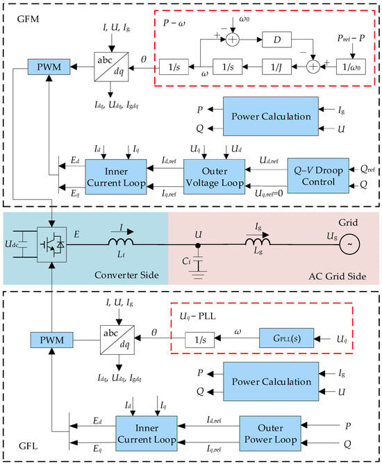
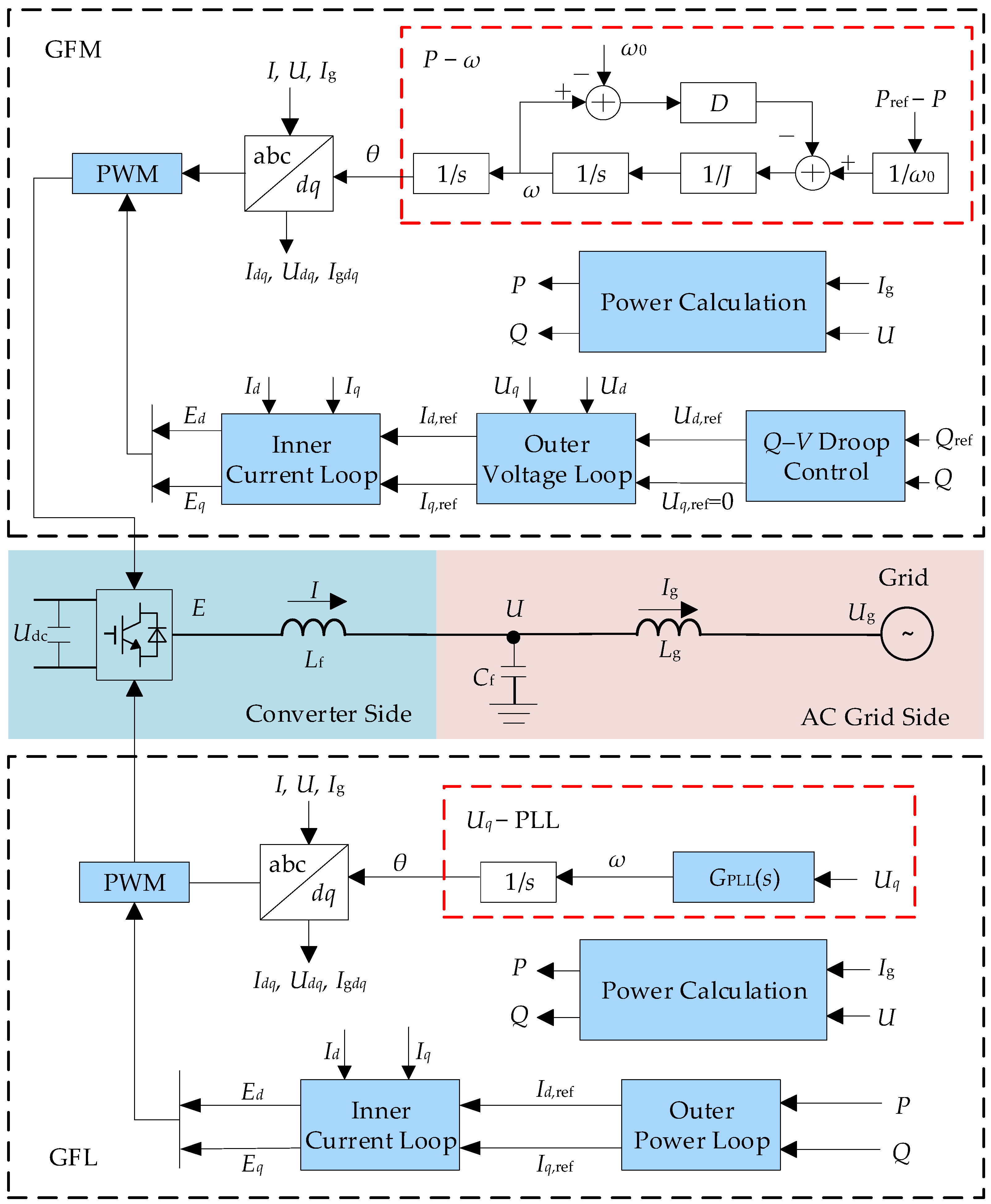
The two converter types use the same three-phase power circuit and pulse-width modulation (PWM), but employ different grid connection control strategies. They are connected through filters and line impedances to the point of common coupling (PCC) and the alternating current (AC) grid. Their control structures are shown in Figure 1.
Figure 1.
Control structures of the GFL and GFM converters.
The variables in Figure 1 are defined as follows. Udc, E, U and Ug denote the direct current side voltage, converter output voltage, PCC voltage, and grid voltage, respectively. I and Ig denote the converter output current and AC grid current, respectively. Lf, Cf and Lg denote the filter inductance, filter capacitance, and AC grid inductance, respectively. GPLL(s) denotes the PLL transfer function of the GFL converter, and ω0 denotes the fundamental system frequency. The variables ω and θ are the angular frequency and phase angle of the synchronously rotating direct-quadrature (dq) reference frame, respectively. D and J denote the damping coefficient and virtual inertia of the GFM synchronization loop, respectively. P, Pref, Q, and Qref denote the active power, active power reference, reactive power, and reactive power reference, respectively. The variables Idq, Udq, Igdq, and Edq denote the dq frame components of I, U, Ig, and E, respectively. Id,ref and Iq,ref denote the d-axis and q-axis current references, respectively. Ud,ref and Uq,ref denote the d-axis and q-axis voltage references generated by the droop controller, respectively.
The converters operate under either grid-following or grid-forming control. The GFL converter employs an outer power loop and an inner current loop and tracks the grid phase through a PLL. Its mathematical model is given by Equation (1).
where GPLL(s) denotes the transfer function of the proportional-integral (PI) controller in the PLL. The functions GP,GFL(s), GQ,GFL(s), and GC,GFL(s) denote the transfer functions of the outer active power, outer reactive power, and inner current control loops, respectively. These transfer functions are defined as
For each controller, the corresponding Kp and Ki terms denote the proportional and integral gains, respectively.
The GFM converter employs Q–V droop control, an outer voltage loop, and an inner current loop, and achieves grid synchronization through virtual synchronous machine control. Its control model is given by Equation (3).
where U0 and Kq denote the voltage reference and Q–V droop coefficient, respectively. The functions GV,GFM(s) and GC,GFM(s) denote the transfer functions of the outer voltage and inner current control loops, respectively. These transfer functions are defined as
For each controller, the corresponding Kp and Ki terms denote the proportional and integral gains, respectively.
2.2. Hybrid System Configuration
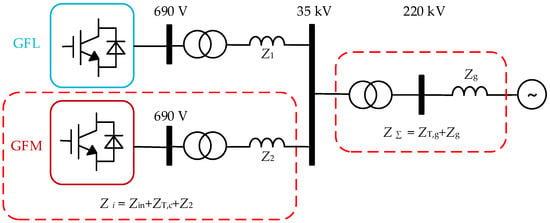
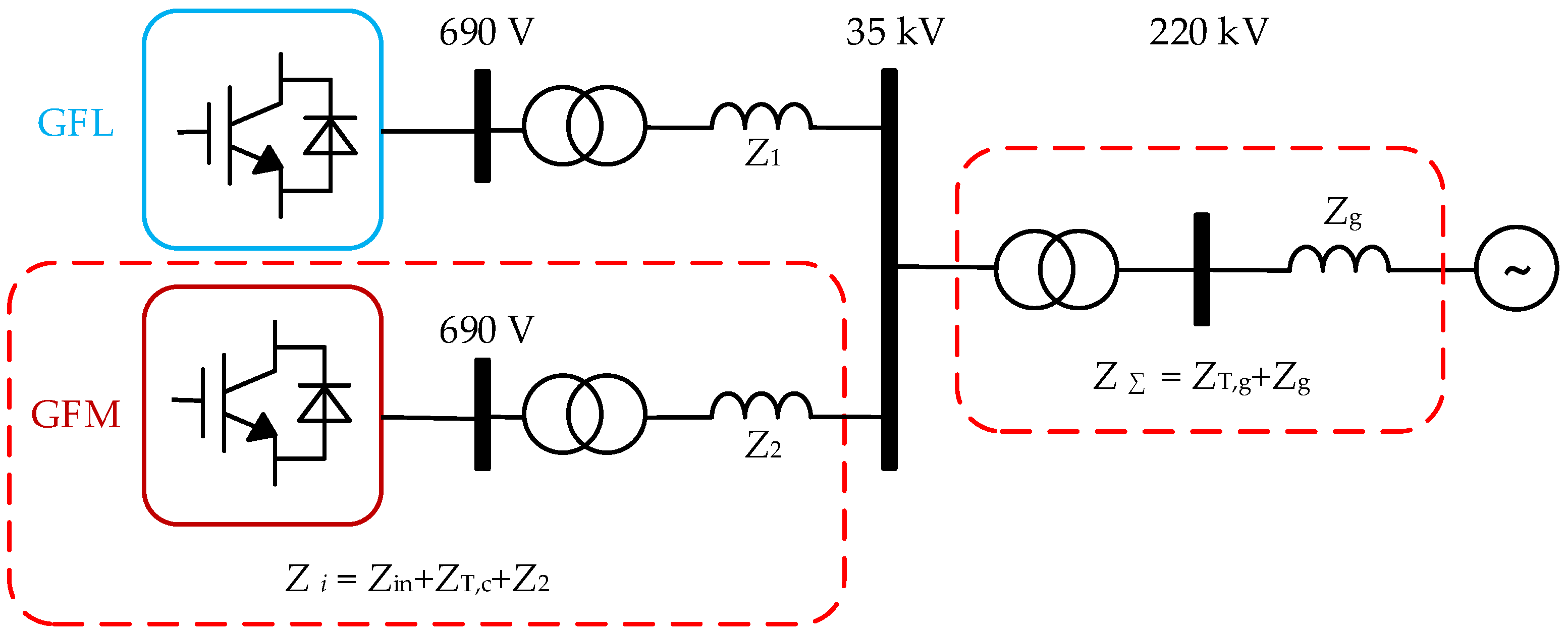
The hybrid wind farm employs both GFL and GFM control strategies. Figure 2 shows the system configuration. The system consists of one equivalent GFL converter and one equivalent GFM converter. Each converter operates at 690 V and is connected to a common 35 kV bus through a 690 V/35 kV step-up transformer. The common 35 kV bus is connected to the 220 kV transmission grid through a 35 kV/220 kV step-up transformer [22,23].
Figure 2.
Schematic diagram of the hybrid GFL and GFM converter system.
Subscripts 1 and 2 refer to the impedances of the GFL and GFM branches, respectively. ZΣ denotes the equivalent impedance seen from the PCC toward the upstream AC grid. It includes the equivalent series impedance ZT,g of the 35 kV/220 kV step-up transformer and the equivalent grid impedance Zg.
Based on the small-signal voltage source representation of the GFM converter [11], the GFM converter and its step-up transformer connected in series can be modeled as an ideal voltage source behind an equivalent internal impedance Zi. The impedance Zi consists of the GFM converter internal impedance Zin, the equivalent series impedance ZT,c of the 690 V/35 kV transformer, and the 35 kV connection branch impedance Z2. The impedance is expressed as Zi = Ri + jXi.
The corresponding admittance is
where Gi is the conductance and Bi is the magnitude of the inductive susceptance of the equivalent GFM branch. The value of Bi quantifies the contribution of the GFM branch to the equivalent system strength. If the branch resistance is neglected and a common per-unit (p.u.) base is adopted, Yi = −j/Xi and Bi = 1/Xi. On the common per-unit base, Bi is a real scalar. It can therefore be combined with SCR0 to derive a scalar expression for the gSCR.
The calculation of Bi establishes a control-parameter-dependent mapping between the dynamic characteristics of the GFM converter and its contribution to the equivalent grid strength. The complete dq impedance matrix is evaluated at the system-specific critical oscillation frequency, with the transformer and line impedances explicitly included. Therefore, the resulting capacity estimate reflects the converter control parameters and the network configuration considered in the analysis.
The following assumptions are made to highlight the stability mechanism at the system level while keeping the model tractable:
- (1)
- Because this study focuses on grid strength at the transmission level, interactions among individual wind turbines are neglected. A single equivalent grid connection point is retained at the plant level. The model includes the PLL, the inner current loop, and the outer active and reactive power loops.
- (2)
- The external AC grid is represented by an infinite bus with constant voltage magnitude and frequency. Its capacity is assumed to be much larger than the capacity of the local wind farm. The infeed bus is connected to the infinite bus through line and transformer impedances. Grid strength is determined jointly by these impedances and the converter capacity connected to the bus.
- (3)
- The study focuses on small-signal stability and grid-forming capability assessment under normal operating conditions. The model retains the dominant factors governing grid strength and converter control behavior. These factors include connected converter capacity and the main control bandwidths. High-frequency switching dynamics, current limiting and saturation associated with severe faults, and other secondary dynamics are omitted. The subsequent time-domain simulations focus on the retained low-frequency electromechanical and control dynamics.
3. Estimation of the GFM Converter Capacity Ratio Using the Generalized Short-Circuit Ratio
A common per-unit system is adopted. The total installed capacity Stotal = 2 MVA and the rated PCC voltage UN = 35 kV are selected as the power and voltage bases, respectively. The total installed capacity is given by
where SGFM and SGFL denote the capacities of the GFM and GFL converters, respectively.
Stotal = SGFM + SGFL,
The GFM converter capacity ratio β is defined as the ratio of the GFM converter capacity to the total installed capacity
Accordingly, the GFM and GFL converter capacities are expressed as SGFM = βStotal and SGFL = (1 − β)Stotal, respectively.
By definition, β ∈ [0, 1]. When β = 0, the system consists entirely of GFL converters. Increasing β shifts capacity from GFL to GFM converters while keeping the total installed capacity constant. Because a nonzero GFL capacity is required for the stability analysis, the subsequent analysis considers 0 ≤ β < 1.
For a single-infeed system connected to an infinite bus, the short-circuit ratio (SCR) is commonly used to characterize grid strength and is defined as
where Sac denotes the short-circuit capacity of the external AC system, and ZΣ,pu denotes the total per-unit impedance seen from the PCC toward the upstream grid.
For a system with multiple converter infeeds, the conventional SCR is extended to the gSCR. The gSCR accounts for the network parameters and the rated capacities of the connected converters. For a single-infeed system, the matrix formulation of the gSCR reduces to the conventional SCR. Hence, gSCR0 = SCR0. The quantity SCR0 denotes the baseline SCR at β = 0 and is determined by the external grid parameters and Stotal. When these quantities are fixed, SCR0 is independent of β. Under a fixed total installed capacity, increasing β reallocates capacity from GFL to GFM converters. Using the common per unit system defined above, the impedances used to evaluate SCR0 and Bi are referred to the common 35 kV PCC. Therefore, SCR0 and Bi represent the baseline grid strength and GFM branch susceptance, respectively, on the same per-unit basis. Based on the equivalent voltage source representation of the GFM converter and the inductive branch assumption, the corresponding source admittance contributions at the PCC are additive. On the common base, the GFM branch contributes βBi, while the remaining GFL capacity is (1 − β)Stotal. Normalizing the total source admittance by the remaining GFL capacity gives [12]
The CSCR is defined as the SCR at which a GFL converter connected to an infinite bus reaches its small-signal stability boundary. For the system with a single-infeed considered here, the critical gSCR is equal to the CSCR. The equivalent external grid impedance is gradually varied for fixed control parameters and a specified steady-state operating point. The CSCR is reached when the dominant complex-conjugate eigenvalue pair first reaches the imaginary axis while all remaining eigenvalues remain in the open left half-plane. The corresponding condition is
where AGFL denotes the state matrix obtained by linearizing the GFL converter system at the specified control parameters and steady-state operating point. The symbol λk denotes the kth eigenvalue of AGFL. The functions α(⋅) and Re(⋅) denote the spectral abscissa and real part, respectively.
Accordingly, the stability boundary is
gSCR(β) ≥ CSCR.
The minimum GFM converter capacity ratio required for small-signal stability is therefore
The target gSCR of the hybrid system is denoted by gSCR*, where gSCR* ≥ CSCR. The capacity ratio that satisfies the target grid strength requirement must satisfy
The corresponding minimum GFM converter capacity ratio required to meet the target grid strength is
In engineering practice, grid strength is often classified empirically according to the SCR. A grid with SCR < 2 is generally classified as very weak, one with 2 ≤ SCR < 3 as weak, and one with SCR ≥ 3 as strong [24]. To ensure that the GFL converter terminal is not connected to a very weak grid, SCR0.69 ≥ 2 is adopted as an auxiliary engineering criterion. This threshold is compared with the CSCR, and the larger of the two thresholds is adopted.
The electrical distance between the 690 V terminal of the GFL converter and the common 35 kV bus is represented by the transformer reactance X0.69/35 = 0.080082 p.u. When this criterion is referred to the common 35 kV bus, the equivalent gSCR threshold becomes gSCR35 = 1/(1/SCR0.69 − X0.69/35) ≥ 2.3814. This threshold is used in the subsequent GFM converter capacity ratio analysis.
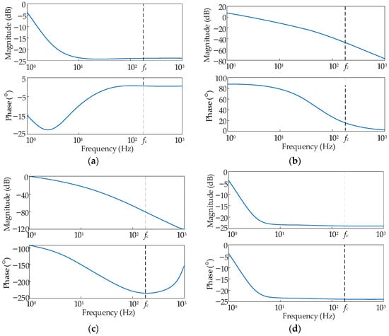
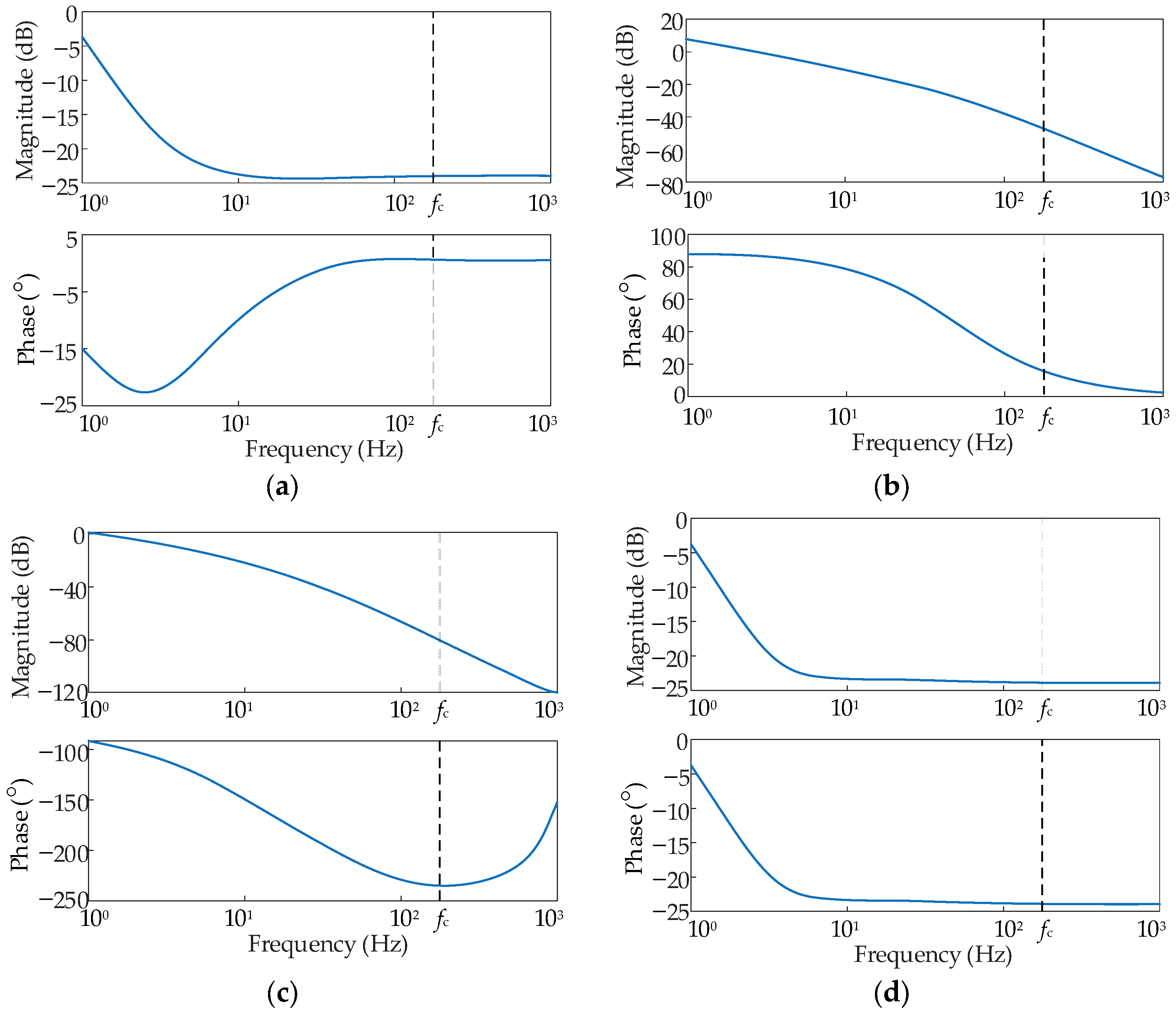
Using the parameters listed in Table A1 of Appendix A, the CSCR is calculated as 2.3984, with a corresponding critical oscillation frequency of fc = 176.86 Hz. The associated critical eigenvalue pair is −0.00044 ± j1111.27 s−1. The PLL states and the d- and q-axis components of the GFL grid current have combined participation factors of 51.79% and 44.64%, respectively. Thus, the critical mode involves coupled PLL synchronization and GFL grid current dynamics. Figure 3 shows that the maximum singular value of the dq impedance matrix at the GFM converter terminal is Using an equivalent inductance model, this value is referred to the fundamental frequency. For f0 = 50 Hz, the equivalent internal reactance is calculated as Xin = 0.014493 p.u.
Figure 3.
Frequency responses of the dq impedance matrix at the GFM converter terminal: (a) Zdd. (b) Zdq. (c) Zqd. (d) Zqq.
Adding the reactances of the 690 V/35 kV transformer and the 35 kV connection branch gives the total GFM branch reactance Xi = 0.094504 p.u. With the branch resistance neglected, Bi = 1/Xi = 10.5816 p.u. The GFL and GFM converters have different 35 kV connection branch inductances. Accordingly, Bi is evaluated from the GFM branch impedance, whereas SCR0 is evaluated from the GFL branch impedance for the all GFL system at β = 0. The initial gSCR at the 35 kV PCC is gSCR0 = SCR0 = 1/|ZΣ,pu| = 2.20.
Table 1 presents the estimated GFM converter capacity ratios for different target gSCR values. Because the initial grid strength is below the CSCR, the minimum GFM converter capacity ratio required for small-signal stability is βmin = 1.53%. When gSCR* is set to 5.00 and 10.00, the corresponding minimum capacity ratios are 17.97% and 37.90%, respectively. These ratios correspond to GFM converter capacities of 0.359 MVA and 0.758 MVA. The results show that a higher target grid strength requires a higher GFM converter capacity ratio.
Table 1.
Estimated minimum GFM converter capacity ratios for the hybrid system.
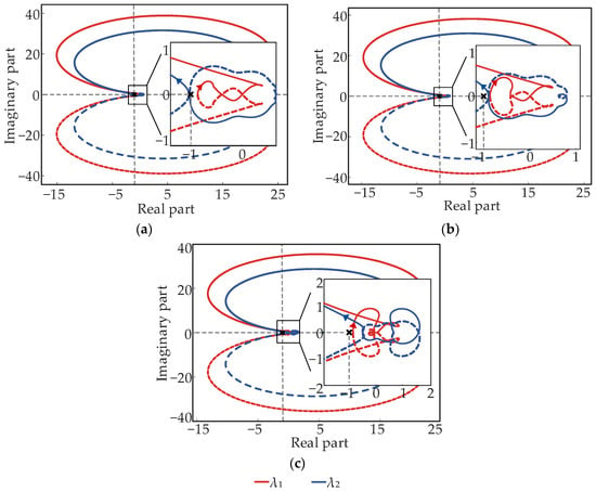
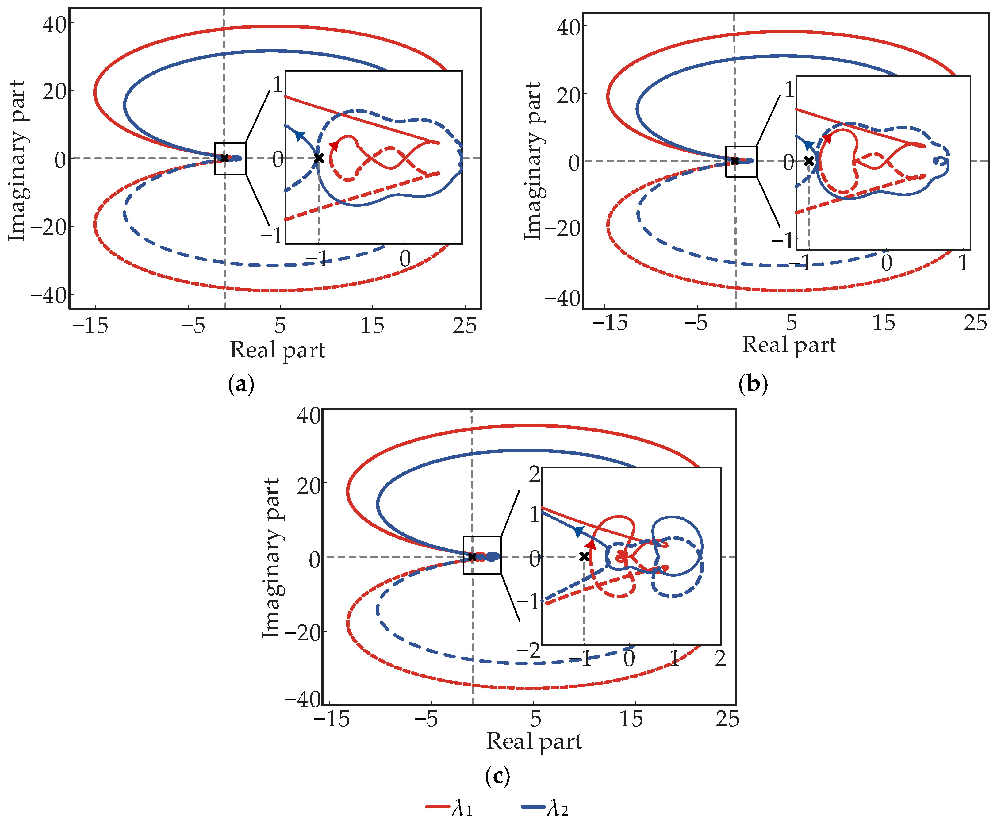
To verify the consistency between the estimated capacity ratios and the stability criterion in the frequency domain, generalized Nyquist analysis is performed for SCR0 = 2.20 at β = 1%, 3%, and 10%. These cases represent a capacity ratio below the continuous lower bound, a ratio above the lower bound, and a higher capacity ratio, respectively.
In Figure 4, the point (−1, j0) serves as the critical point in the complex plane. Clockwise net encirclements are counted as positive, whereas counterclockwise net encirclements are counted as negative. The quantities λ1 and λ2 denote the eigenvalues of the return ratio matrix, and their trajectories form the characteristic loci. The return ratio matrix has no poles in the right half-plane under the specified parameters. When β = 1%, the characteristic loci encircle the critical point twice clockwise. The closed loop therefore has two poles in the right half-plane and is unstable. For β = 3% and 10%, the characteristic loci do not encircle the critical point. The corresponding closed loops have no poles in the right half-plane and are stable. For all three cases, the generalized Nyquist results are consistent with the analytical capacity ratio estimate.
Figure 4.
Generalized Nyquist plots for different GFM converter capacity ratios: (a) β = 1%. (b) β = 3%. (c) β = 10%.
To further assess the continuous lower bound on the GFM converter capacity ratio, β is varied continuously at SCR0 = 2.20, and the eigenvalues of the linearized closed-loop model of the hybrid system are calculated. The critical eigenvalue pair reaches the imaginary axis at a GFM converter capacity ratio of 1.3578%. The estimated minimum GFM converter capacity ratio of 1.5282% differs from this boundary by 0.1704 percentage points, and all eigenvalues remain in the left half-plane at the estimated value.
4. Assessment of Grid-Forming Capability Using Normalized Margins and a Bottleneck Index
The gSCR characterizes the equivalent grid strength of the hybrid system for a given GFM converter capacity ratio and set of branch parameters. However, neither the GFM converter capacity ratio nor the gSCR alone provides a comprehensive assessment of grid-forming capability. A comprehensive assessment therefore also needs to account for time-domain dynamic performance. Accordingly, a grid-forming capability assessment framework for the hybrid system is developed based on four categories of factors, including system strength, the GFM converter capacity ratio, control parameters, and disturbance response. These factors are further organized into three assessment levels corresponding to basic support conditions, control parameter effects, and disturbance response performance [17].
where u denotes the configuration and control parameter vector and y denotes the grid-forming capability index vector. The index ζ denotes the equivalent damping ratio. The quantities ΔPpk, ΔQpk, and Δfpk are the peak deviations in active power, reactive power, and frequency following a disturbance, respectively. Rf,max denotes the peak RoCoF, and Ts denotes the settling or recovery time following a disturbance. The simulations use a fixed-step solver with a step size of 1 μs.
The basic support conditions are characterized by the gSCR and β. The gSCR reflects the combined effects of grid impedance and connected capacity, whereas β denotes the GFM converter capacity ratio. Indices derived from the SCR directly characterize the relative strengths of the AC system and power electronic equipment and therefore serve as primary metrics for assessing voltage support strength. For grid-connected power electronic equipment, however, the SCR alone cannot characterize all stability issues. System impedance, equipment control characteristics, and dynamic responses must also be considered.
Control parameter effects are assessed using Kp,PLL, Ki,PLL, J, and D. These parameters are varied to determine their effects on synchronization dynamics, inertial response, and oscillation damping. Capacity optimization methods based solely on the SCR cannot capture the influence of control parameters on the capacity ratio boundary.
The disturbance response performance is characterized by ζ, ΔPpk, ΔQpk, Δfpk, Rf,max, and Ts. These indices are used to assess oscillation damping, frequency support, and power recovery following small disturbances and load switching events.
For a response variable x, the peak deviation and settling time are defined by
where x ∈ {P, Q, f}. The quantity Δxpk denotes the maximum absolute deviation of x from its post-disturbance steady-state value. The quantity ts(ε) denotes the time at which the response first enters the settling band and remains within it thereafter. The quantities t0 and x∞ denote the time at which the disturbance is applied or cleared and the post-disturbance steady-state value, respectively. The quantity εx denotes the absolute settling band for x.
The peak RoCoF, logarithmic decrement, and damping ratio are defined by
where Ak = |x(tk) − x∞| and Ak+1 = |x(tk+1) − x∞| denote the amplitudes of two successive peaks in the same direction relative to the steady-state value. The quantity δ denotes the logarithmic decrement. The expression for ζ is based on a single dominant underdamped mode or an approximately second-order response.
For operating cases in which both active and reactive power responses are available, ζ = min{ζP, ζQ} and Ts = max{Ts,P, Ts,Q} are used to characterize the least favorable oscillation damping and the slowest recovery process, respectively.
The screening criteria are assigned to the corresponding response variables and disturbance scenarios. For the 5% three-phase symmetrical voltage sag cases, the dominant mode damping ratio is estimated from the active and reactive power responses at the PCC after the disturbance, with a lower threshold of ζlim = 0.050 [25]. The power settling time is measured from the clearance of the voltage sag until both responses enter and remain within their respective absolute settling bands of 0.020 p.u. [26]. With reference to the 0.150 s dynamic response interval in [27], Tlim = 0.150 s is adopted as a threshold specific to this study for the settling time metric defined in Equation (16). For the 0.1 p.u. load step cases, the peak frequency deviation and peak RoCoF are calculated from the GFM converter frequency, with thresholds of Δfpk,lim = 0.100 Hz [28] and Rlim = 2.00 Hz/s [29], respectively. In the PLL parameter study, Δfpk instead denotes the peak deviation of the frequency estimated by the GFL converter PLL following the voltage sag, and the same numerical threshold of Δfpk,lim = 0.100 Hz is applied.
To account for differences in units and numerical scales, each grid-forming capability index is normalized by its corresponding threshold. For indices for which larger values indicate better performance, such as the damping ratio and system strength, the normalized margin is defined as the ratio of the calculated value to the lower threshold. For indices for which smaller values indicate better performance, such as frequency deviation, RoCoF, and settling time, the normalized margin is defined as the ratio of the upper threshold to the calculated value. Consequently, the dimensional response quantities are evaluated using dimensionless normalized margins relative to their corresponding thresholds rather than being compared directly. These margins are defined by
where m denotes the operating case. The five quantities , , , , and denote the system strength margin, damping margin, frequency deviation margin, RoCoF margin, and settling time margin, respectively.
Accordingly, unity defines the constraint boundary for each normalized index. A value greater than unity indicates that the corresponding requirement is satisfied with a positive margin. A value equal to unity indicates operation at the constraint boundary. A value less than unity indicates that the corresponding requirement is not satisfied.
where the quantity denotes the bottleneck index for grid-forming capability under operating case m. The quantity denotes the normalized margin of index i. The set 𝒜(m) ⊆ {g, ζ, f, R, T} contains the indices applicable to operating case m.
By definition,
Thus, is equivalent to all applicable indices satisfying their respective constraints for operating case m. The bottleneck index is defined as the minimum of the applicable normalized margins. The method introduces no subjective weights and does not allow an index with satisfactory performance to compensate for an index that fails to meet its requirement. Moreover, indicates only that the indices selected in this study for operating case m satisfy their respective screening criteria. It does not certify that the equipment complies with a comprehensive grid-forming interconnection standard.
By jointly considering basic support conditions, control parameter effects, and disturbance response performance, the method provides a quantitative basis for assessing grid-forming capability through simulations and determining the GFM converter capacity ratio in hybrid GFL and GFM converter systems.
5. Simulation Studies
To validate the proposed GFM converter capacity ratio estimation method and grid-forming capability assessment framework for a hybrid GFL and GFM converter system, a simulation model is developed in MATLAB/Simulink R2022b. Power oscillations, frequency support, and recovery performance following disturbances are compared under different capacity ratios, grid strengths, control parameters, and disturbance scenarios. For each operating case, the applicable indices are selected based on the available response curves. The applicable index sets are 𝒜(m) = {g, ζ, T} for the capacity ratio and grid strength studies, 𝒜(m) = {f} for the PLL parameter studies, and 𝒜(m) = {f, R} for the virtual inertia and damping coefficient studies. The bottleneck index is calculated using Equation (19). Throughout this section, all normalized margins and bottleneck indices are calculated using unrounded simulation data. The simulation parameters are provided in Table A1 of Appendix A.
5.1. Verification of Small-Disturbance Grid-Forming Capability Under Different Capacity Ratios
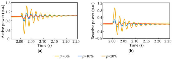
To examine the effect of the GFM converter capacity ratio on the small-disturbance grid-forming capability of the hybrid system, the initial SCR is fixed at SCR0 = 2.20. The quantity β is set to 3%, 10%, and 20%, yielding gSCR values of 3.42, 4.51, and 6.40, respectively. At t = 2.0 s, a 5% three-phase symmetrical voltage sag is applied at the infinite bus and cleared after 10 ms. The active and reactive power responses at the PCC are shown in Figure 5.
Figure 5.
Active and reactive power responses at the PCC under different GFM converter capacity ratios: (a) active power response; (b) reactive power response.
As shown in Figure 5, for β = 3%, 10%, and 20%, the values of are 1.426, 1.880, and 2.668, respectively. All three values satisfy . The corresponding peak power deviations max{ΔPpk, ΔQpk} are 0.915 p.u., 0.250 p.u., and 0.131 p.u. As β increases from 3% to 10% and then to 20%, the peak power deviation decreases by approximately 72.7% and 47.6%, respectively. The values of ζ are 0.062, 0.065, and 0.092, and the corresponding values are 1.246, 1.304, and 1.836. All three values exceed unity. Thus, the small-disturbance oscillations at all three capacity ratios decay with damping that meets the prescribed lower limit. The settling times Ts for the absolute settling band are approximately 0.202 s, 0.142 s, and 0.119 s. The corresponding values are 0.743, 1.060, and 1.266. The corresponding bottleneck index values are 0.743, 1.060, and 1.266. At β = 3%, the bottleneck index is determined by the settling time margin and is less than unity. At β = 10% and 20%, all applicable indices satisfy their respective constraints.
These results quantitatively demonstrate that, under the specified operating conditions, increasing the GFM converter capacity ratio increases the equivalent gSCR, improves oscillation damping, reduces the peak power deviation, and shortens the settling time.
5.2. Verification of Small-Disturbance Grid-Forming Capability Under Different Grid Strengths
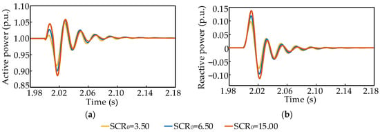
To analyze the influence of grid strength on the grid-forming capability of the hybrid system, the equivalent grid impedance is varied to establish different initial SCR values. With β fixed at 20%, SCR0 is set to 3.50, 6.50, and 15.00, yielding gSCR values of 7.02, 10.77, and 21.40, respectively. At t = 2.0s, a 5% three-phase symmetrical voltage sag is applied at the infinite bus and cleared after 10 ms. The active and reactive power responses at the PCC are shown in Figure 6.
Figure 6.
Active and reactive power responses at the PCC under different grid strengths: (a) active power response; (b) reactive power response.
As shown in Figure 6, for SCR0 = 3.50, 6.50, and 15.00, the values of are 2.927, 4.490, and 8.923, respectively. All three values satisfy and increase markedly with grid strength. The corresponding peak power deviations max{ΔPpk,ΔQpk} are 0.102 p.u., 0.123 p.u., and 0.142 p.u., respectively, indicating a slight increase in the peak power deviation as grid strength increases. The values of ζ are 0.107, 0.128, and 0.155, and the corresponding values are 2.149, 2.566, and 3.092. All three values exceed unity. As gSCR increases, the oscillations decay more rapidly, indicating improved small-disturbance damping. The settling times Ts for the absolute settling band are 0.063 s, 0.051 s, and 0.051 s. The corresponding MT values are 2.398, 2.955, and 2.947. The corresponding bottleneck index values are 2.149, 2.566, and 2.947. All applicable indices satisfy their respective constraints in the three grid strength cases.
These results show that increasing grid strength increases the system strength and oscillation damping margins, although it may slightly increase the peak power deviation immediately after the disturbance.
5.3. Verification of Small-Disturbance Grid-Forming Capability Under Different Control Parameters
To further examine the influence of control parameters on the small-disturbance grid-forming capability of the hybrid system, the PLL parameters of the GFL converter and the virtual inertia J, damping coefficient D, and Q–V droop coefficient Kq of the GFM converter are varied. The PLL-estimated frequency, RoCoF, and active power responses are compared. In all simulations, SCR0 and β are fixed at 2.20 and 20%, respectively, and the remaining parameters are unchanged.
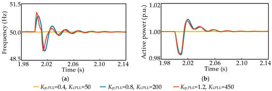
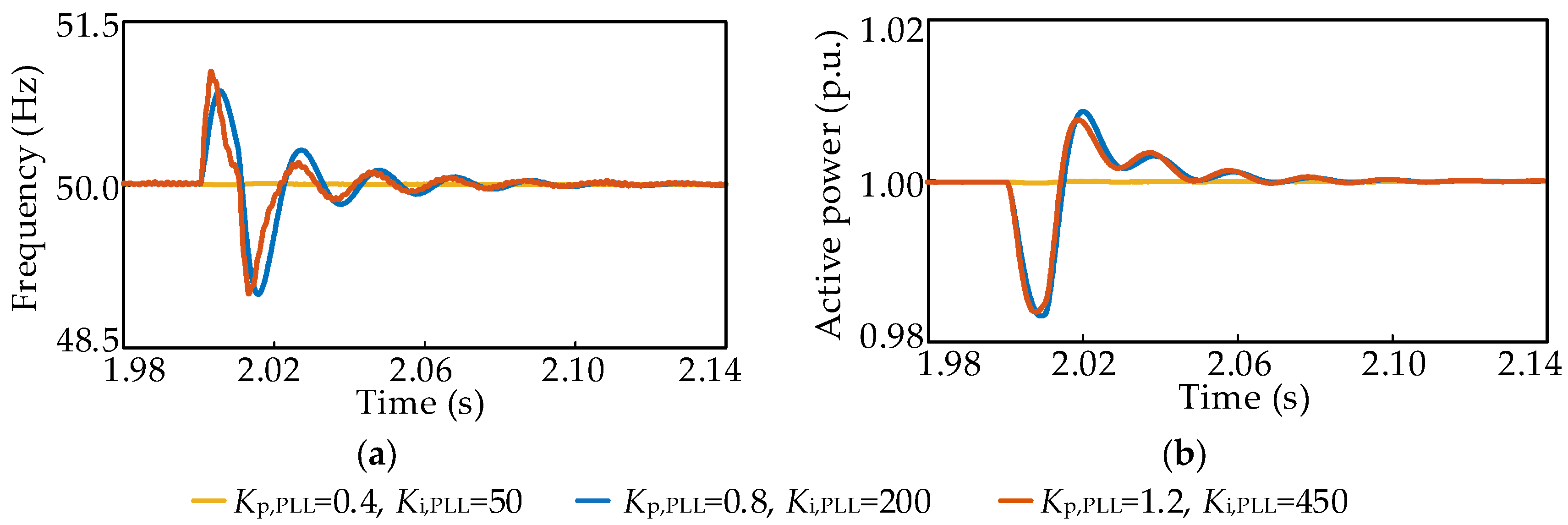
First, to analyze the influence of PLL parameters on the small-disturbance grid-forming capability of the hybrid system, three sets of PLL proportional and integral gains are compared. At t = 2.0s, a 5% three-phase symmetrical voltage sag is applied at the infinite bus and cleared after 10 ms. The PLL-estimated frequency and active power responses of the GFL converter are shown in Figure 7.
Figure 7.
PLL-estimated frequency and active power responses of the GFL converter under different PLL parameters: (a) PLL-estimated frequency response; (b) active power response.
As shown in Figure 7, for the three sets of PLL parameters, the values of Δfpk are 0.014 Hz, 1.007 Hz, and 1.044 Hz, respectively. The corresponding values are 7.047, 0.099, and 0.096. Only the first PLL parameter set satisfies the frequency deviation constraint. The maximum active power deviations are 0.00026 p.u., 0.01676 p.u., and 0.01626 p.u., respectively. Because 𝒜(m) = {f}, the bottleneck index satisfies .
The results show that, under weak grid conditions, simultaneously increasing the PLL proportional and integral gains increases the maximum deviation of the PLL-estimated frequency. Thus, higher PLL gains increase the system sensitivity to voltage disturbances and amplify the PLL-estimated frequency deviation.
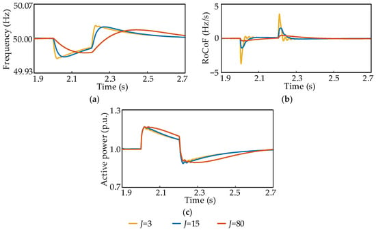
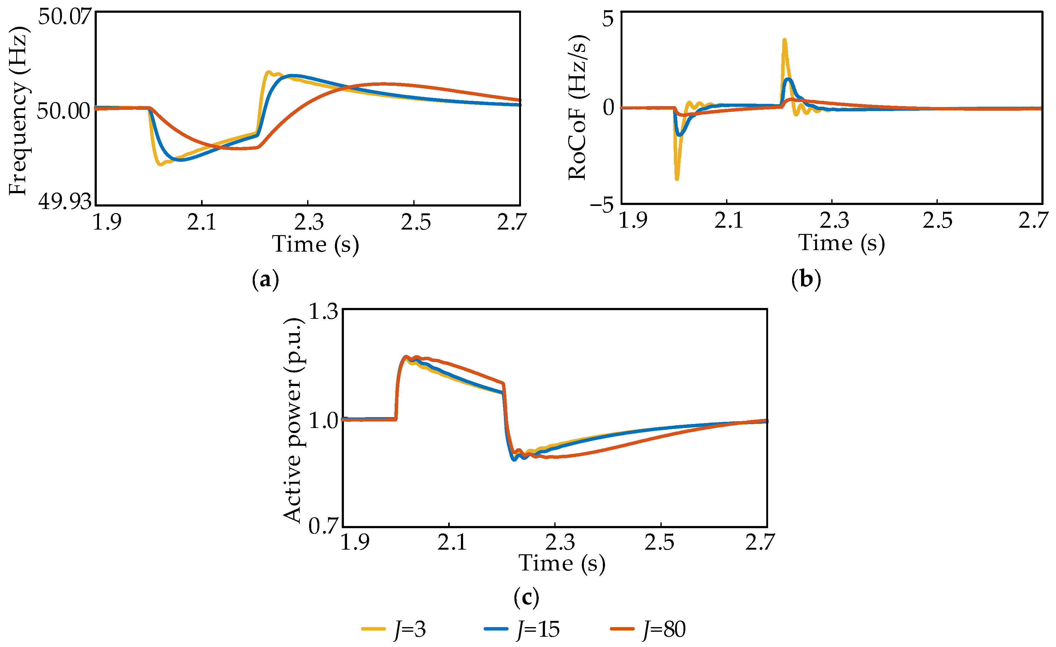
Second, to examine the influence of J on frequency support and power recovery, three virtual inertia values are considered. At t = 2.0 s, a 0.1 p.u. active power load disturbance is applied at the PCC and removed after 0.2 s. The frequency, RoCoF, and active power responses of the GFM converter are shown in Figure 8.
Figure 8.
GFM output responses for different virtual inertia values: (a) frequency response; (b) RoCoF response; (c) active power response.
As shown in Figure 8, for J = 3, 15, and 80, the values of Δfpk are 0.040 Hz, 0.037 Hz, and 0.029 Hz, respectively. All three values are below the 0.100 Hz limit. The corresponding values are 2.470, 2.695, and 3.463. The values of Rf,max are 3.714 Hz/s, 1.501 Hz/s, and 0.454 Hz/s, respectively. The corresponding values are 0.539, 1.333, and 4.408. The values of ΔPpk are 0.164 p.u., 0.169 p.u., and 0.169 p.u., respectively. The corresponding bottleneck index values are 0.539, 1.333, and 3.463. At J = 3, the RoCoF margin determines the bottleneck index, which is below unity and therefore does not satisfy the constraint. At J = 15 and 80, all applicable indices satisfy their respective constraints.
These results show that, within the specified parameter range, increasing J substantially reduces the RoCoF and improves frequency support but also slows active power recovery. The results quantitatively reveal the tradeoff between inertial support and active power recovery speed.
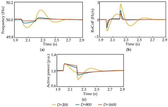
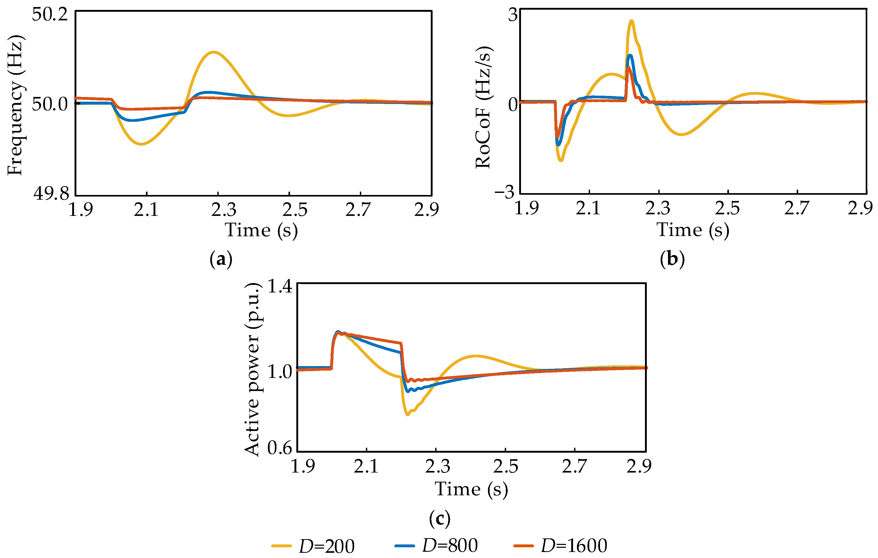
Third, to examine the influence of D on oscillation damping and active power recovery, three damping coefficients are considered. At t = 2.0 s, a 0.1 p.u. active power load disturbance is applied at the PCC and removed after 0.2 s. The frequency, RoCoF, and active power responses of the GFM converter are shown in Figure 9.
Figure 9.
GFM output responses for different damping coefficients: (a) frequency response; (b) RoCoF response; (c) active power response.
As shown in Figure 9, for D = 200, 800, and 1600, the values of Δfpk are 0.111 Hz, 0.037 Hz, and 0.013 Hz, respectively. The corresponding values are 0.902, 2.693, and 7.821. The values of Rf,max are 2.620 Hz/s, 1.501 Hz/s, and 1.152 Hz/s, respectively. The corresponding values are 0.763, 1.332, and 1.736. At D = 200, neither the frequency deviation index nor the RoCoF index satisfies its constraint. At D = 800 and 1600, both indices satisfy their respective constraints. The values of ΔPpk are 0.225 p.u., 0.170 p.u., and 0.165 p.u., respectively. The corresponding bottleneck index values are 0.763, 1.332, and 1.736. For all three values of D, the RoCoF margin determines the bottleneck index.
These results show that increasing the damping coefficient markedly suppresses frequency and active power oscillations and increases both the frequency deviation and RoCoF margins. However, as D increases, the active power takes progressively longer to enter the allowable steady-state error band, indicating a tradeoff between enhanced damping and active power recovery speed.
Finally, the influence of the Q–V droop coefficient Kq is assessed under the voltage sag condition. The values Kq = 0.0025, 0.0050, and 0.0100 are considered. Over the investigated range, the PCC voltage magnitude and GFM converter reactive power response exhibit only marginal variations.
In summary, within the specified parameter range, the PLL parameters of the GFL converter primarily affect synchronization dynamics and the magnitude of power oscillations. The virtual inertia of the GFM converter mainly affects the RoCoF and inertial support capability. The damping coefficient primarily determines the attenuation of post-disturbance oscillations. Proper coordination of the GFL and GFM converter control parameters is therefore essential for improving the small-disturbance grid-forming capability of the hybrid system.
6. Conclusions
This paper proposes a GFM converter capacity ratio estimation method and a grid-forming capability assessment framework for a hybrid GFL and GFM converter system with a fixed total installed capacity. The main conclusions are as follows.
- (1)
- By combining the CSCR of the GFL converter with the terminal impedance of the GFM converter, a relationship between the GFM converter capacity ratio and gSCR is established. This relationship yields a continuous lower bound on the GFM converter capacity ratio that satisfies both the small-signal stability and target grid strength requirements. In the case study, the capacity ratio lower bound required for small-signal stability is 1.53%. For target gSCR values of 5.00 and 10.00, the required capacity ratios are 17.97% and 37.90%, respectively. Under the selected operating conditions, the stability results obtained using the generalized Nyquist criterion are consistent with the capacity ratio estimates.
- (2)
- Normalized margins and the bottleneck index are used to assess system strength, oscillation damping, frequency support, and settling time. The framework determines whether each index satisfies its requirement and identifies the factor that limits system performance. In the case study, increasing the GFM converter capacity ratio increases the equivalent gSCR, improves oscillation damping, reduces the peak power deviation, and shortens the settling time. Increasing the external grid strength increases the system strength and oscillation damping margins but slightly increases the peak power deviation immediately after a disturbance. Thus, neither the capacity ratio nor gSCR alone can fully characterize the dynamic performance of the system.
- (3)
- The control parameters affect the dynamic response of the hybrid system in different ways. Higher PLL gains increase the sensitivity of the GFL converter to voltage disturbances and amplify the PLL-estimated frequency deviation. Increasing virtual inertia reduces the RoCoF but slows active power recovery. Increasing the damping coefficient suppresses frequency and active power oscillations, but higher damping may also slow active power recovery. The GFM converter capacity ratio and control parameters should therefore be coordinated with grid strength and dynamic performance requirements.
The proposed method and framework link preliminary GFM converter capacity ratio estimation with grid-forming capability assessment and can provide guidance for capacity planning and control parameter design in hybrid renewable energy plants. This study adopts a single-infeed equivalent model and focuses primarily on small-disturbance conditions. Future work will examine the framework under multi-infeed configurations and broader disturbance conditions. It will also validate the proposed approach through controller-hardware-in-the-loop testing and experimental studies.
7. Patents
The following Chinese invention patent applications have resulted from the work reported in this manuscript:
- (1)
- Zhu, L.; Wu, M.H.; Guo, L.; Li, X.L.; Liu, Y.X.; Jia, N.J.; Cao, J.C.; Zeng, G.M.; Liu, Y.Y.; Zhu, Y.H.; Tang, Y.H.; Luo, C. Capacity Proportioning Method for a Hybrid System of Grid-Following and Grid-Forming Converters for Renewable Energy Stations. Chinese Invention Patent Application No. 202610884535.2, filed on 18 June 2026 (pending).
- (2)
- Zhu, L.; Wu, M.H.; Guo, L.; Li, X.L.; Liu, Y.X.; Cao, J.C.; Jia, N.J.; Zeng, G.M.; Tang, Y.H.; Zhu, Y.H.; Liu, Y.Y.; Luo, C. Grid-Forming Capability Evaluation Method Based on System Strength, Control Dynamics, and Disturbance Response. Chinese Invention Patent Application No. 202610884534.8, filed on 18 June 2026 (pending).
Author Contributions
Conceptualization, M.W. and L.Z.; methodology, M.W., L.Z. and X.L.; software, M.W. and J.C.; validation, J.C.; formal analysis, M.W. and J.C.; investigation, X.L.; resources, L.Z.; data curation, M.W.; writing—original draft preparation, M.W. and J.C.; writing—review and editing, L.Z., X.L. and L.G.; visualization, M.W. and J.C.; supervision, L.Z., X.L. and L.G.; project administration, L.Z., X.L. and L.G.; funding acquisition, L.Z. All authors have read and agreed to the published version of the manuscript.
Funding
This research was funded by the Smart Grid-National Science and Technology Major Project, grant number 2025ZD0804200.
Data Availability Statement
The original contributions presented in the study are included in the article, further inquiries can be directed to the corresponding author.
Conflicts of Interest
The authors declare no conflicts of interest.
Abbreviations
The following abbreviations are used in this manuscript:
| GFL | Grid-following |
| GFM | Grid-forming |
| PLL | Phase-locked loop |
| gSCR | Generalized short-circuit ratio |
| CSCR | Critical short-circuit ratio |
| RoCoF | Rate of change of frequency |
| PWM | Pulse-width modulation |
| PCC | Point of common coupling |
| AC | Alternating current |
| dq | Direct-quadrature |
| PI | Proportional-integral |
| SCR | Short-circuit ratio |
| p.u. | Per unit |
Appendix A
Table A1.
Simulation parameters of the hybrid GFL and GFM converter system.
References
- Zheng, X.; Yang, S.; Xie, Z.; Zhang, X. Equivalence of Grid-Tied Inverters Operating in the Grid-Following and Grid-Forming Modes just Through Adapting the Control Parameters. IEEE Trans. Energy Convers. 2026, 1–12. [Google Scholar] [CrossRef] [Scilit]
- Aljarrah, R.; Fawaz, B.B.; Salem, Q.; Karimi, M.; Marzooghi, H.; Azizipanah-Abarghooee, R. Issues and challenges of grid-following converters interfacing renewable energy sources in low inertia systems: A review. IEEE Access 2024, 12, 5534–5561. [Google Scholar] [CrossRef] [Scilit]
- Li, Y.; Gu, Y.; Green, T.C. Revisiting Grid-Forming and Grid-Following Inverters: A Duality Theory. IEEE Trans. Power Syst. 2022, 37, 4541–4554. [Google Scholar] [CrossRef] [Scilit]
- Wu, C.; Lyu, Y.; Wang, Y.; Blaabjerg, F. Transient Synchronization Stability Analysis of Grid-Following Converter Considering the Coupling Effect of Current Loop and Phase Locked Loop. IEEE Trans. Energy Convers. 2024, 39, 544–554. [Google Scholar] [CrossRef] [Scilit]
- Zhou, W.; Mohammed, N.; Bahrani, B. Voltage and current dynamics cancellation of weak-grid-tied grid-following inverters for maximum transferable power improvement. IEEE Trans. Energy Convers. 2024, 39, 2053–2067. [Google Scholar] [CrossRef] [Scilit]
- Elshenawy, M.A.; Radwan, A.A.A.; Mohamed, Y.A.-R.I. Analysis and Weakening of Sequence Impedance Coupling in Grid-Forming Converters. IEEE Trans. Power Deliv. 2024, 39, 3292–3304. [Google Scholar] [CrossRef] [Scilit]
- Gonzalez-Cajigas, A.; Roldan-Perez, J.; Bueno, E.J. Design and Analysis of Parallel-Connected Grid-Forming Virtual Synchronous Machines for Island and Grid-Connected Applications. IEEE Trans. Power Electron. 2022, 37, 5107–5121. [Google Scholar] [CrossRef] [Scilit]
- Liu, H.; He, X.; Qing, H.; Qiu, C.; Chen, Y.; Geng, H. Decision-Making of GFM/GFL Capacity Ratio: Ensuring Small-Signal and Frequency Stability. IEEE Trans. Ind. Appl. 2026, 1–12. [Google Scholar] [CrossRef] [Scilit]
- Liyanage, C.; Meegahapola, L.; Nutkani, I.; Jalili, M. A techno-economic optimisation framework for grid-forming battery inverter sizing in renewable dominant power grids. J. Energy Storage 2026, 144, 119704. [Google Scholar] [CrossRef] [Scilit]
- Dong, W.; Xin, H.; Wu, D.; Huang, L. Small Signal Stability Analysis of Multi-Infeed Power Electronic Systems Based on Grid Strength Assessment. IEEE Trans. Power Syst. 2019, 34, 1393–1403. [Google Scholar] [CrossRef] [Scilit]
- Yang, C.; Huang, L.; Xin, H.; Ju, P. Placing Grid-Forming Converters to Enhance Small Signal Stability of PLL-Integrated Power Systems. IEEE Trans. Power Syst. 2021, 36, 3563–3573. [Google Scholar] [CrossRef] [Scilit]
- Xin, H.; Liu, C.; Chen, X.; Wang, Y.; Prieto-Araujo, E.; Huang, L. How Many Grid-Forming Converters Do We Need? A Perspective from Small Signal Stability and Power Grid Strength. IEEE Trans. Power Syst. 2025, 40, 623–635. [Google Scholar] [CrossRef] [Scilit]
- Wang, K.; Li, J. Suppression Method of Sub/Super-Synchronous Oscillation in Direct-Drive Wind Farms Based on a Hybrid GFL-GFM Control Configuration. Energies 2026, 19, 2661. [Google Scholar] [CrossRef] [Scilit]
- Eberlein, S.; Rudion, K. Impact of Inner Control Loops on Small-Signal Stability and Model-Order Reduction of Grid-Forming Converters. IEEE Trans. Smart Grid 2023, 14, 2812–2824. [Google Scholar] [CrossRef] [Scilit]
- Singh, A.; Debusschere, V.; Hadjsaid, N.; Legrand, X.; Bouzigon, B. Slow-Interaction Converter-Driven Stability in the Distribution Grid: Small-Signal Stability Analysis with Grid-Following and Grid-Forming Inverters. IEEE Trans. Power Syst. 2024, 39, 4521–4536. [Google Scholar] [CrossRef] [Scilit]
- Shi, Q.; Dong, W.; Wang, G.; Ma, J.; Wang, C.; Guo, X.; Terzija, V. Grid Strength Assessment Method for Evaluating Small-Signal Synchronization Stability of Grid-Following and Grid-Forming Converters Integrated Systems. J. Mod. Power Syst. Clean Energy 2025, 13, 55–65. [Google Scholar] [CrossRef] [Scilit]
- Wang, Y.; Ruan, L.; Yang, M.; Xiao, X.; Chen, S.; Gomis-Bellmunt, O. Control Interaction Analysis of Hybrid System with Grid-Following and Grid-Forming Inverters Based on Admittance Decomposition. Int. J. Electr. Power Energy Syst. 2024, 162, 110267. [Google Scholar] [CrossRef] [Scilit]
- Liu, N.; Wang, H.; Sun, L.; Zhou, W.; Song, J.; Zhou, D.; Wang, W.; Chen, Z. Modular Impedance Modeling and Stability Analysis of Hybrid AC/DC Power Systems with Grid-Forming and Grid-Following Converters. IEEE Access 2024, 12, 4063–4077. [Google Scholar] [CrossRef] [Scilit]
- Prastiantono, A.; Ramadhan, U.F.; Kim, D.; Hur, D.; Yoon, M. Evaluating Frequency Stability with a Generic Model for IBR Penetration and the Implementation of Grid-Forming Control Strategies. Energies 2024, 17, 2779. [Google Scholar] [CrossRef] [Scilit]
- Hadjileonidas, A.; Li, Y.; Green, T.C. Comparative Analysis of Transient Stability of Grid-Forming and Grid-Following Inverters. In Proceedings of the 2022 IEEE International Power Electronics and Application Conference and Exposition (PEAC), Xiamen, China, 4–7 November 2022; pp. 296–301. [Google Scholar] [CrossRef] [Scilit]
- Li, T.; Wang, P.; Chen, F.; Gu, T.; Yang, D.; Yan, G.; Ma, Z.; Yuan, H. Active Support Performance of Grid-Connected Multi-Power Conversion System Based on Grid-Following/Grid-Forming Control. In Proceedings of the 2024 IEEE Vehicle Power and Propulsion Conference (VPPC); IEEE: New York, NY, USA, 2024; pp. 1–6. [Google Scholar] [CrossRef] [Scilit]
- Burton, T.; Jenkins, N.; Sharpe, D.; Bossanyi, E. Wind Energy Handbook, 2nd ed.; John Wiley & Sons: Chichester, UK, 2011; ISBN 978-0-470-69975-1. [Google Scholar] [CrossRef] [Scilit]
- Li, B.; Liu, J.; Wang, X.; Zhao, L. Fault Studies and Distance Protection of Transmission Lines Connected to DFIG-Based Wind Farms. Appl. Sci. 2018, 8, 562. [Google Scholar] [CrossRef] [Scilit]
- Yu, G.; Hu, Y.; Liu, C.; Tang, B.; Xin, H.; Ma, J.; Cui, G. Research on the Coordinated Optimization Configuration Method for Hybrid Multi-infeed Systems with Grid-following or Grid-forming. Proc. CSEE 2025, 45, 588–601. (In Chinese) [Google Scholar] [CrossRef]
- CIGRE Working Group C4.56. Electromagnetic Transient Simulation Models for Large-Scale System Impact Studies in Power Systems Having a High Penetration of Inverter-Connected Generation; Technical Brochure 881; CIGRE: Paris, France, 2022. [Google Scholar]
- T/CNESA 1008-2023; Technical Specification for Grid-Forming Energy Storage Converters. China Energy Storage Alliance: Beijing, China, 2023. (In Chinese)
- NB/T 32004-2018; Technical Specification for Photovoltaic Grid-Connected Inverters. China Electric Power Press: Beijing, China, 2018. (In Chinese)
- T/CERS 0067-2024/T/EPTC 005-2024; Test Procedure for Grid Connection Behavior of Grid-Forming Wind Turbine Generator. China Energy Research Society and Zhongguancun Smart Power Industry Technology Alliance: Beijing, China, 2024. (In Chinese)
- National Grid ESO. GC0137: Minimum Specification Required for Provision of GB Grid Forming Capability (Formerly Virtual Synchronous Machine Capability); Final Modification Report; National Grid ESO: Warwick, UK, 2021.

Disclaimer/Publisher’s Note: The statements, opinions and data contained in all publications are solely those of the individual author(s) and contributor(s) and not of MDPI and/or the editor(s). MDPI and/or the editor(s) disclaim responsibility for any injury to people or property resulting from any ideas, methods, instructions or products referred to in the content. |
© 2026 by the authors. Licensee MDPI, Basel, Switzerland. This article is an open access article distributed under the terms and conditions of the Creative Commons Attribution (CC BY) license.