A 1D CNN with Exact Grouped SHAP Attribution for Transformer Magnetizing Inrush Identification

Abstract

Reliable transformer differential protection requires fast discrimination between magnetizing inrush and internal faults in the presence of residual flux, harmonic voltage, direct current (DC) bias, measurement noise, and current-transformer (CT) saturation. This study develops a compact one-dimensional convolutional neural network (1D CNN) that acts directly on a three-phase differential-current window and interprets its decision with exact grouped SHAP. A calibrated 50 kVA, 10 kV/400 V, 50 Hz three-limb model was implemented in MATLAB R2023b; to remove an alignment shortcut, event onsets were randomized over the window for both classes on a balanced, independently split data set. At the default decision threshold the CNN reached 91.11% accuracy with 99.26% inrush recall and 82.96% specificity (AUC 0.9833) on an independent test set. Selecting the threshold on the validation set raised accuracy to 94.81% and specificity to 91.11% without materially changing inrush recall. The compact direct-sequence model matched a recurrent LSTM, while an image CNN traded lower inrush recall for higher specificity; both learned models were far more stable than fixed second-harmonic and dead-angle criteria, and the CNN retained competitive performance on windows as short as 10–20 ms. Exact grouped SHAP, recomputed over all correctly classified records with a multi-record background and onset-binned controls, yields a cautious phase-time interpretation rather than a claim of universal field performance.

1. Introduction

Transformer energization imposes a flux trajectory determined by the time integral of the applied winding voltage and the residual flux present at contact making. When the resulting operating point crosses the knee of the magnetization curve, the incremental inductance collapses and a large asymmetric magnetizing current appears. Because this current enters the differential protection circuit as an unbalanced quantity, it can resemble an internal fault and delay or block protection unless the discrimination logic is both selective and fast [1,2,3,4].

Conventional criteria exploit second-harmonic content, waveform dead angle, symmetry, or flux restraint [5,6]. These quantities have direct physical meaning, but fixed thresholds become fragile when modern core material reduces the second-harmonic ratio, when a current-transformer saturates, or when residual flux and distorted voltage reshape the first cycle. Inrush may alternatively be avoided at the source by controlled point-on-wave switching, but this requires breaker coordination and known residual flux rather than a discrimination rule [7]. Data-driven methods reduce dependence on a single threshold.

Early learned-method studies trained artificial neural networks on hand-engineered harmonic and waveform features to discriminate magnetizing inrush from internal faults [8,9], and related protection schemes extended this with two-terminal, support-vector, and multi-classifier approaches [10,11,12,13]. More recent deep-neural, graph-recurrent, denoising, and discriminative-feature-focused convolutional models continue to raise the reported accuracy on simulated and laboratory records [14,15,16,17,18], as reviewed in [19].

These studies confirm the value of learned transient features, but they also leave two practical questions: whether an image transformation or recurrent attention module is necessary for a short three-phase window, and whether the learned decision can be related to a phase and physical time interval. To address the first question under controlled conditions, we compare the direct 1D CNN with a recurrent LSTM and a Gramian-angular-summation-field (GASF) image CNN, and we also evaluate the fixed second-harmonic and dead-angle criteria that motivate the study. Recent feature-transfer CNN work shows that a model trained on simulated waveforms may require explicit cross-transformer adaptation before it can be trusted on measurements [20]. The broader 1D-CNN literature shows that temporal convolutions can learn local morphology without converting a signal into an image [21]. The present study therefore treats the direct-sequence model as a controlled simulation benchmark, in which the architecture and reference-rule comparisons can be measured, rather than as a field-ready relay.

The protection objective is asymmetric. A false-positive inrush decision may delay tripping for an actual internal fault, whereas a false internal-fault decision during energization can produce an unnecessary trip and interrupt restoration. Consequently, a single scalar accuracy can conceal the engineering cost of the error pattern. Inrush recall, fault specificity, probability calibration, and response time should be interpreted together. The operating point is also not fixed by the classifier alone: a relay may combine the learned probability with a restraint current, a differential slope, a minimum dwell time, and a blocking timer. The present work reports the complete confusion structure so that these downstream choices remain visible rather than being absorbed into an unexplained threshold.

A second concern is data provenance. Simulation is attractive because rare energization and internal-fault combinations are difficult to collect under safe operating conditions, but a flexible simulator can accidentally encode the class label through an unphysical shortcut. For example, if every inrush waveform starts at the first sample while every fault begins later, a network can obtain high accuracy by detecting the window boundary instead of learning magnetic or electrical morphology. We therefore randomize the onset for both classes, retain a common prefault background, and apply prefix occlusion after training. This audit does not prove that no shortcut exists, but it makes one especially plausible shortcut measurable.

A third concern is the interpretation of learned evidence. Harmonic ratios and dead-angle indices are easy to map to a protection rule, whereas a convolutional feature map is not. An explanation method should therefore preserve the physical axes of the signal, state its background choice, and report its numerical additivity error. Grouped SHAP is used here because a phase and a 10 ms interval are more meaningful protection units than individual samples or hidden neurons. The explanation is deliberately presented as conditional evidence for this model family; it is not used to claim that the network has discovered a new universal magnetic law.

The contributions are: (1) a reproducible MATLAB R2023b pipeline that couples a calibrated nonlinear three-limb inrush model with internal-fault and measurement-channel models; (2) a compact 1D CNN operating directly on the three-phase sequence, with controlled comparisons against a recurrent LSTM and a GASF-image CNN and against fixed second-harmonic and dead-angle rules; (3) an explicit random-onset design and prefix-occlusion control to expose alignment leakage; (4) matched comparisons with RBF SVM, bagged-tree, and KNN baselines plus out-of-distribution stress tests and a validation-set decision threshold; (5) a report of short-window performance and an architecture-selection ablation; and (6) exact grouped Shapley attribution over all correctly classified phase-time records with a multi-record background and onset-binned pairing. The data split, seed, parameter ranges, and generated result tables are saved by the MATLAB script.

2. Theoretical Basis of Transformer Inrush Identification

2.1. Formation Mechanism and Confusing Characteristics of Magnetizing Inrush

For phase k, flux continuity requires the post-closing flux linkage to start from the residual state. The exact winding relation is

$${\psi }_k\left(t\right)={\psi }_{r,k}+{\int }_{t_0}^t\left(u_k\left(\tau \right)-R_{1,k}{i}_k\left(\tau \right)\right)\mathit{d\tau }$$

(1)

where ψ_r,k is the residual linkage, u_k is terminal voltage, R_1,k is winding resistance, and i_k is phase current. During the initial high-inductance interval, the resistive drop is small and the prospective flux is governed mainly by the voltage integral. Harmonic order h contributes to flux approximately in proportion to 1/h; its phase at contact making determines whether it compresses or expands the active saturation margin [3,4]. A DC current does not enter the voltage integral. It displaces the magnetic operating point through magnetomotive force and reduces the directional margin to the knee.

$$i_{m,k}=a_k{\psi }_{e,k}+b_k\mathrm{sgn}\left({\psi }_{e,k}\right){\left(\max \left(\left|{\psi }_{e,k}\right|-{\psi }_{\mathrm{sat},k}\right),0\right)}^q$$

(2)

Equation (2) is the reduced single-valued magnetic backbone used in the simulation. Coefficient a_k represents the linear magnetizing slope, b_k and q determine the post-knee rise, and ψ_e,k is the phase-dependent knee linkage. The three-limb constraint removes zero-sequence drift from both the integrated flux and the DC-induced displacement. This coupling transfers a saturation event in one limb into the return paths of the other two, so a protection criterion based on only phase A can miss the dominant limb [3,4].

The closing angle and residual flux enter the same initial-condition problem but are not interchangeable. The voltage integral is phase shifted by the breaker command, while residual flux is an initial state that persists through the switching instant. A closing angle that would be benign for zero residual flux can therefore be severe when the core retains flux in the same direction. Conversely, a large residual vector can be partly canceled by a favorable voltage integral. The random generator samples both quantities independently within a zero-sum three-limb subspace, allowing the data to contain mild, moderate, and strongly saturated cases without assigning the outcome to one scalar feature. This is important for a learning model because the relevant evidence is a trajectory in state space rather than a fixed harmonic ratio.

The zero-sum constraint is a deliberate simplification of a three-limb core. It enforces a physically plausible return-flux relationship and prevents the numerical integrator from accumulating a common-mode flux that is not supported by the assumed winding connection. The constraint also creates cross-phase dependence: the phase with the largest excursion is not independent of the other two phase currents. In a real transformer, tank geometry, winding connection, structural steel, and zero-sequence paths modify this relation. The model should therefore be read as a controlled backbone that exposes the interaction of residual flux, nonlinear magnetization, and circuit impedance, not as a substitute for a finite-element or hysteresis-resolved core model.

From a protection perspective, an internal fault differs in its energy source and persistence. Fault current is driven by the network voltage through a low-impedance fault path and usually remains present over consecutive cycles until the breaker or protection clears it. Inrush current is driven by temporary magnetic saturation; its largest pulses are phase dependent and tend to decay as the flux trajectory moves back toward the normal operating region. Nevertheless, CT saturation can make a fault appear pulse-like, while harmonic voltage or DC bias can make inrush more continuous. This overlap explains why the study uses complete three-phase windows and explicitly perturbs the measurement channel instead of assuming an ideal primary current.

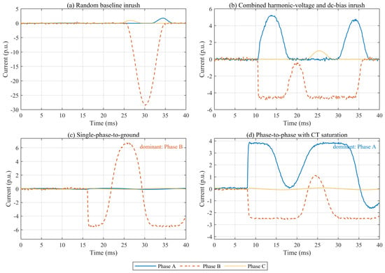
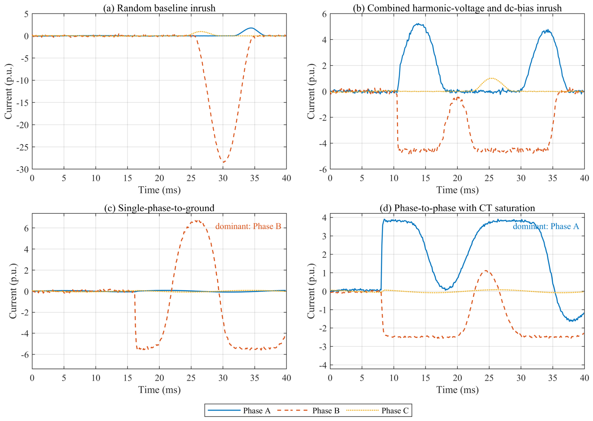
Internal faults can share the high magnitude, DC offset, and harmonic content of an inrush waveform. The principal discriminating evidence is therefore distributed over time: an inrush record tends to exhibit phase-selective, unipolar saturation pulses separated by low-current intervals, whereas fault current is more nearly continuous after inception and its decaying-DC offset follows the network X/R ratio. The measurement channel can narrow this distinction by soft-clipping the fault waveform and making the positive and negative half-cycles unequal. Figure 1 illustrates four randomly generated records; the event onset is different in every record and is not used as a class label. The current base is the 2.887 A-rated high-voltage current, so the plotted values are in per unit on that base.

Figure 1. Randomly generated 40 ms classification-window records on the 2.887 A-rated HV current base: (a) baseline inrush; (b) combined harmonic-voltage and DC-bias inrush; (c) the sampled internal-fault type; and (d) the sampled internal-fault type with asymmetric soft CT saturation. Both classes use a common low-amplitude prefault background and independently sampled event onsets. All panels use one physical p.u. ordinate; solid, dashed, and dotted lines identify phases A, B, and C so that the small non-dominant phases are not visually rescaled to the dominant fault phase. In panel (c), the non-faulted phases remain below 0.08 p.u.

2.2. CNN Deep-Feature Extraction from Current Sequences

Each example is a matrix X ∈ ℝ^3×320, corresponding to phases A, B, and C over a 40 ms window sampled at 8 kHz. Statistics used for z-score normalization are computed only from the training subset and then applied unchanged to validation, test, and robustness records. A one-dimensional convolution with kernel w scans along time while retaining the channel relationship:

$$z_{j,t}=\sigma \left(\sum w_{j,c,\tau }{x}_{c,t+\tau }+b_j\right)$$

(3)

Here, j indexes the output channel, c indexes the three input phases, τ indexes the temporal kernel, and σ is the rectified linear activation. The first nine-sample kernels capture local edges and pulse widths over 1.125 ms at the 8 kHz input rate. The subsequent five- and three-sample kernels combine these responses after two stride-two pooling operations, giving the final representation a receptive field that spans both local pulse shape and its neighboring half-cycle. Global average pooling replaces a large fully connected feature map with 64 channel averages and reduces the number of parameters that can memorize sample-specific timing. The one-dimensional temporal implementation follows the sequence-CNN perspective summarized in [21], while the convolutional formulation is consistent with established gradient-based feature learning and image-CNN foundations [22,23]. The final Softmax layer returns the inrush and fault probabilities.

The architecture is intentionally small relative to image-based or recurrent protection networks. A wider network could fit more nuisance variation, but it would also increase the opportunity to memorize the synthetic generator and make attribution more difficult. The first convolution sees all three channels at each temporal location, so phase relationships can be represented before pooling discards fine time resolution. The second and third blocks operate on progressively more abstract patterns: combinations of pulse edges, polarity changes, and inter-phase imbalance. Batch normalization stabilizes the scale of these intermediate responses, while dropout acts only before the final classifier and is disabled during inference. Global average pooling makes the class score depend on distributed evidence across the window rather than on one fully connected position, which is consistent with the randomized-onset design.

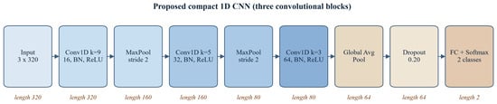
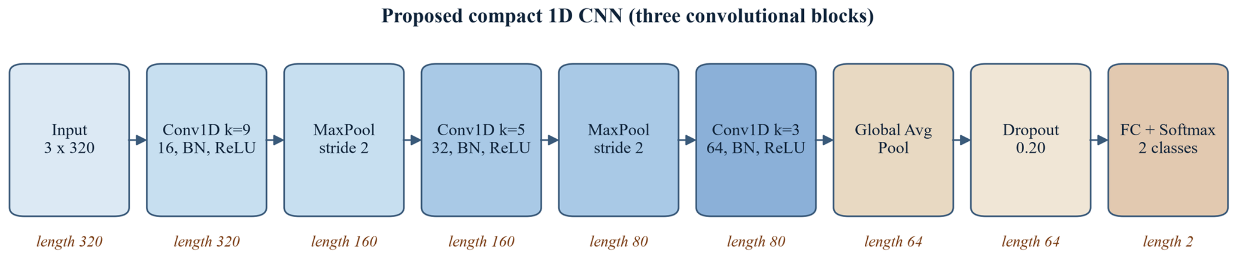
The sequence representation also clarifies what is and is not compared with the baselines.As shown in Figure 2, the CNN receives 960 normalized current values (three phases×320 samples per phase) and learns its own filters through three convolutional blocks, followed by global average pooling, dropout, and a two-class Softmax head. The SVM, bagged trees, and KNN receive 14 descriptors selected before training. The comparison therefore tests two deployment philosophies: direct waveform learning and a compact hand-designed feature pipeline. It is not a parameter-matched contest, because each baseline has a different inductive bias and different sensitivity to scale. Reporting all four models is useful because a slightly less accurate model may still be preferred if it has lower memory, simpler calibration, or a better-known failure mode in a relay implementation.

Figure 2. Proposed 1D CNN architecture. The displayed tensor lengths are 320-160-80 before global average pooling; batch normalization and ReLU follow each convolution, and dropout is applied before the final classifier.

2.3. SHAP Model-Interpretability Theory

The 40 ms record is partitioned into four 10 ms segments for each phase, producing M = 12 interpretable groups whose index set is G = {1, …, M}. A coalition contains selected phase-time groups from the query sample while all unselected groups are taken from an opposite-class reference sample. For the classifier output f and group j, the exact Shapley value is

$${\phi }_j={\sum }_{S\subseteq G\setminus \left\{j\right\}}{\displaystyle \frac{\left|S\right|!\left(M-\left|S\right|-1\right)!}{M!}}\left(f\left(S\cup \left\{j\right\}\right)-f\left(S\right)\right)$$

(4)

All 2¹² coalitions are evaluated, rather than approximated by random sampling. This is tractable for 12 groups and guarantees the efficiency relation f(x) − f(x_ref) = Σⱼ φⱼ up to floating-point error. Positive values increase the inrush probability relative to the reference; negative values support the fault class. Grouping also avoids assigning physical meaning to individual hidden neurons: every attribution corresponds directly to one phase and one 10 ms interval. The additive attribution follows the SHAP formulation and its later model-interpretability development [24,25]. The reported residual is retained as an implementation check, not as an independent performance claim.

The opposite-class median is used as a transparent reference rather than a zero waveform. A zero reference would create an artificial discontinuity because the classifier was trained on records with a low-amplitude prefault background and because current magnitude itself carries physical information. The median reference preserves a typical waveform for the other class while suppressing an individual record’s random onset, noise, and CT realization. This choice makes the question precise: which phase-time groups move the query probability away from a typical opposite-class record? A different background, such as an unconditional training median, would answer a different question and could change the sign or magnitude of individual contributions.

Grouped attribution has two practical advantages for protection research. First, it reduces 960 sample-level contributions to 12 values that can be displayed without implying sample-level causality. Second, the groups align with a half-cycle-scale inspection interval, so an engineer can compare a highlighted region with the corresponding current trace, harmonic content, or relay time budget. The interpretation remains local: a positive 20–30 ms contribution means that replacing the reference in that group increased the CNN’s inrush probability for the selected query. It does not mean that the interval is sufficient by itself or that the same interval will dominate another transformer, seed, or operating point.

3. Simulation Model and Experimental Configuration

3.1. Three-Phase Transformer Model and Parameter Validation

The inrush generator represents a 50 kVA, 10 kV/400 V, 50 Hz, Yyn0 transformer using three nonlinear limb branches, winding resistance, leakage reactance, and a shared zero-sum flux constraint. The coefficients follow the transient-model formulation in [3], while the implementation here is a reduced single-valued magnetic backbone intended for controlled classification experiments. A fixed-step fourth-order Runge–Kutta solver uses 20 microseconds for physical simulation; the simulated current is subsequently resampled for the classifier. Table 1 lists the parameters that define the common current base and nonlinear closure. All current figures use the rated high-voltage current I_HV = S/(√3V_HV) = 2.887 A as the p.u. base; the corresponding low-voltage current is 72.17 A. Although 50 kVA units are commonly protected by fuses in distribution practice, this rating is retained because it matches the small distribution and station-service auxiliary transformers widely used in differential-relay demonstrations and laboratory test sets, and it gives a numerically reproducible down-scaled benchmark; the morphology and the learned features are reported in per-unit and phase-time terms so the method can be re-evaluated at larger ratings.

Table 1. Transformer and numerical parameters used in the MATLAB model.

Parameter	Value	Parameter	Value
Rated frequency	50 Hz	Rated capacity	50 kVA
Voltage ratio and vector group	10 kV/400 V, Yyn0	Rated HV/LV current	2.887/72.17 A
Series resistance	0.0212 p.u.	Leakage reactance	0.0395 p.u.
Knee flux A/B/C	0.900/0.900/1.071 p.u.	Linear slope ak	0.012 p.u./p.u.
Post-knee gain bk A/B/C	20.14/121.12/7.61	Post-knee exponent q	2.2
DC flux gain A/B/C	6.67/18.00/6.43	Physical time step	20 microseconds

In Equation (2), a_k is the linear slope listed in Table 1, b_k is the post-knee gain, q is the common exponent, and ψ_sat,k is the phase-specific knee flux. The unusually large B-limb gain is retained from the reference parameterization and compensates for the zero-sum three-limb closure; it is a reduced-model coefficient rather than a universal material constant. Model validation uses the same residual-flux vector, 60 degree closing command, harmonic phases, and DC-current commands as the reference study. The single calibration factor establishes the high-voltage current base from the baseline case; the harmonic, which is DC-biased, and combined cases are then predictions. Table 2 shows that all four peaks agree within 0.14%. This is a consistency check against the reference model, not an experimental validation of a physical transformer.

Table 2. Peak-current consistency check at the 60 degree breaker-command angle.

Condition	Reference Peak (A)	MATLAB Peak (A)	Relative Error (%)
Baseline	21.3000	21.3000	0.0000
Harmonic voltage	32.1900	32.1472	−0.1329
DC bias	35.1500	35.1498	−0.0005
Combined	41.6700	41.6643	−0.0138

The reference peaks are those reported for the calibrated 50 kVA model. The same baseline-derived current conversion is applied to the remaining three cases.

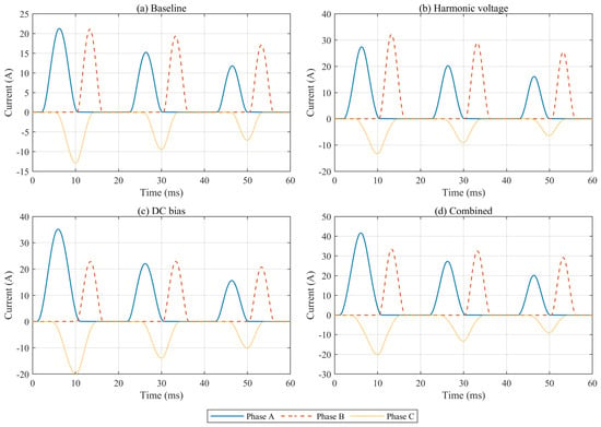
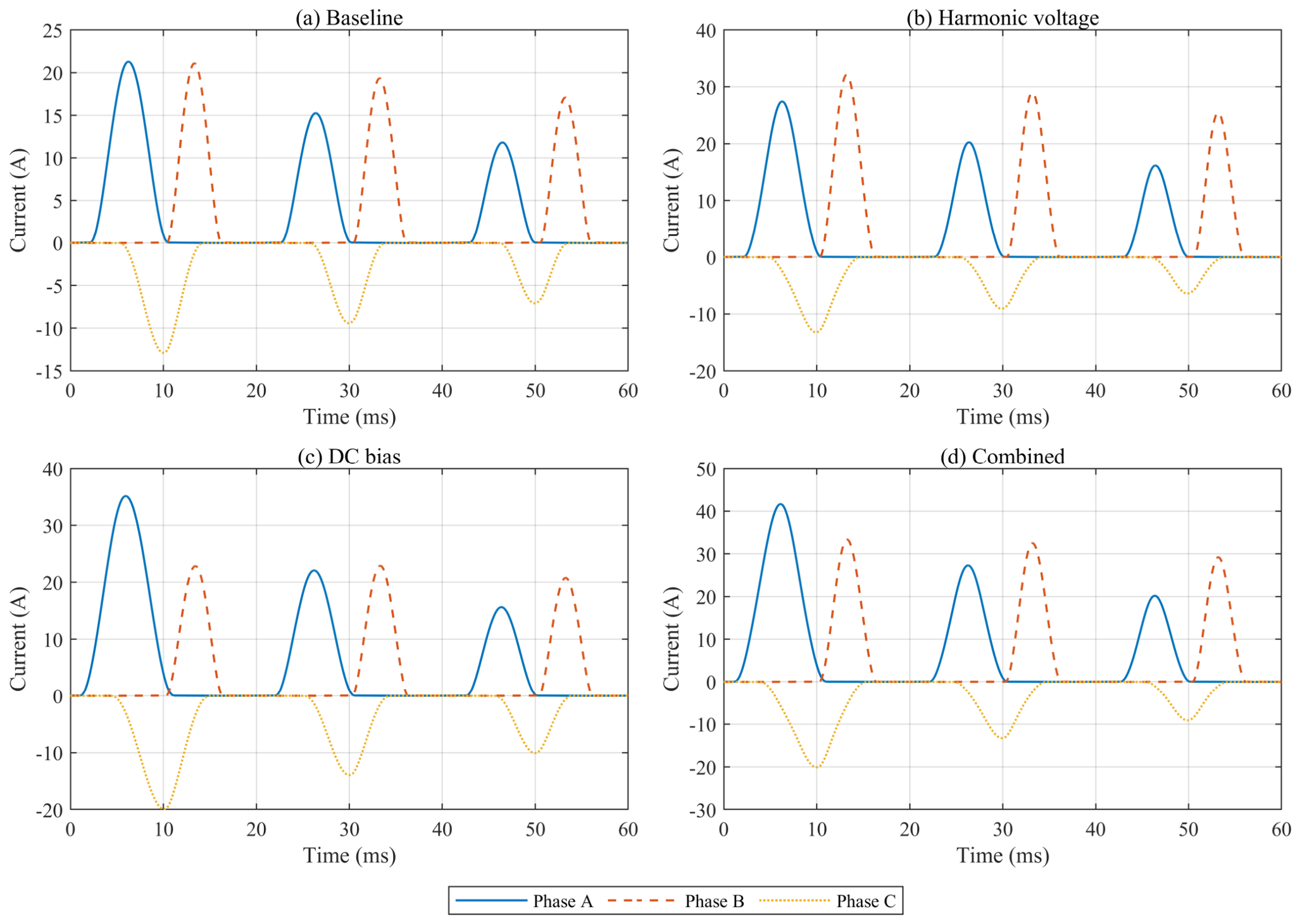
The corresponding three-phase validation waveforms are shown in Figure 3. Unlike Figure 1, this figure deliberately uses the fixed 60 degree reference realization and an extended 60 ms view so that the physical-model comparison is not confused with the randomized 40 ms classification records.

Figure 3. Fixed-reference three-phase model-validation waveforms at 60 degrees in an extended 60 ms view: (a) baseline; (b) harmonic voltage; (c) DC bias; and (d) combined harmonic-voltage and DC-bias disturbance. The classification window used elsewhere is the first 40 ms. Phase A, B, and C use consistent blue, red, and yellow colors with solid, dashed, and dotted line styles.

3.2. Complex Disturbance Conditions and Data Set Construction

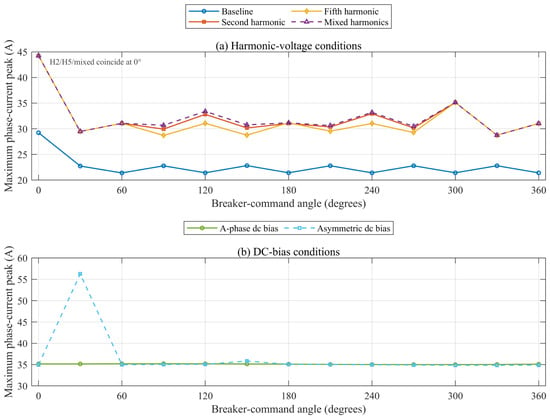
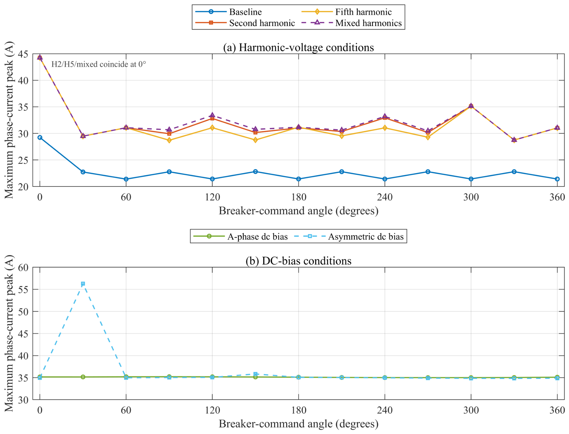
Two complementary data sources define the study. First, 117 saved operating-point files, each containing one valid closing-angle realization, together hold 85,292 admissible combinations of the closing angle, three-phase residual flux, harmonic condition, and DC-bias pattern. These records store peak currents rather than full waveforms, so they are used only to confirm the disturbance envelope and to set physically relevant sampling ranges; they are not used to train or test the classifier. Figure 4 shows an important feature of this envelope: after taking the maximum over residual-flux combinations, the baseline and harmonic-voltage curves are comparatively flat with respect to the command angle, whereas an asymmetric DC-bias combination produces a single 56.27 A peak at 30 degrees. The 0 and 360 degree endpoints are not identical because the saved files contain different discrete combination sets at those endpoints; the figure is therefore an operating-range envelope, not a periodicity test.

Figure 4. Operating-range envelope from the retained 117-file sweep: (a) harmonic-voltage conditions; (b) DC-bias conditions. Each point is the maximum over the residual-flux combinations stored for that 30 degree command angle and disturbance condition; the envelope is broadly flat, while the 30 degree asymmetric DC-bias combination reaches 56.27 A. At 0 degrees, the second-harmonic, fifth-harmonic, and mixed-harmonic peaks are identical, so their markers overlap rather than indicating a missing second-harmonic point. The 0 and 360 degree endpoints are retained as separate file collections and therefore need not coincide.

Second, full 40 ms three-phase records are generated for classification. Inrush cases randomly vary command angle, residual-flux polarity and magnitude, source resistance, leakage reactance, knee flux, post-knee gain, second- and fifth-harmonic magnitude and phase, differential DC bias, noise, and CT saturation. Internal-fault cases include single-phase-to-ground, phase-to-phase, two-phase-to-ground, and three-phase faults. Their waveforms include a decaying-DC offset, second-harmonic distortion, optional half-cycle deformation, noise, and an asymmetric tanh-based CT channel. The fault inception angle is uniform on 0–360 degrees. Most importantly, the event onset is sampled independently and uniformly from the 0–40 ms classification window for both classes. Before onset, both classes contain a common low-amplitude prefault sinusoidal background; a five-sample transition ramp avoids a class-specific step artifact. Thus t = 0 does not identify the class, and the manifest records Onset_ms for auditability. The complete ranges are summarized in Table 3.

Table 3. Classification data set and disturbance ranges.

Item	Setting	Purpose
Input window	3 phases × 320 samples; 8 kHz; 40 ms	Two 50 Hz cycles; p.u. base 2.887 A HV
Class balance	900 inrush and 900 internal-fault records	Balanced binary task
Data split	70% training; 15% validation; 15% test	Independent model selection and testing
Inrush harmonics	H2: 0.05–0.15 p.u.; H5: 0.03–0.08 p.u.; random phase	Source distortion
Residual flux	Random zero-sum vector; maximum 0.15–0.85 p.u.	Magnetic memory
DC command	0.03–0.15 p.u.; single-phase or asymmetric	Operating-point displacement
Fault types	SLG, LL, LLG, and three-phase; inception 0–360 deg	Internal-fault diversity
Event onset	Uniform 0–40 ms for both classes; common prefault background	Alignment-control design
Nominal noise	28–42 dB SNR; additive white sample noise	Measurement uncertainty
CT saturation	Asymmetric soft tanh; negative knee 0.65 × positive; level 3–9 p.u.	Measurement-channel distortion
Shifted sets	SNR 18–25 dB; f = 47–53 Hz; parameters ±25%	Out-of-distribution stress

The randomization is structured rather than unconstrained. Residual-flux vectors are projected to a zero-sum subspace and scaled so that their maximum absolute component lies between 0.15 and 0.85 p.u.; this keeps the magnetic state within the intended operating envelope while allowing different dominant limbs. Source frequency is varied around 50 Hz, and the resistance, leakage reactance, knee, and post-knee gains are perturbed independently for the nominal family. Harmonic amplitudes are only activated for the corresponding scenario branches, so the generator retains interpretable cases such as baseline, second harmonic, fifth harmonic, mixed harmonic, DC bias, and combined disturbance. Fault masks are sampled from four topologies and are then multiplied by independently drawn alternating current (AC) amplitude, decaying-DC ratio, time constant, and optional half-cycle gate. Each record therefore has a traceable physical cause for its variability.

The disturbance sets are generated after the nominal model has been fit and are not used to tune the CNN. The low-SNR set changes only the noise range, the frequency-shift set changes the source-frequency range, the CT set forces the asymmetric soft-saturation channel for both labels, and the parameter-shift set broadens the circuit and magnetic coefficients. This separation matters because evaluating a model on data that were repeatedly inspected during tuning can make robustness appear stronger than it is. The five seed runs repeat this complete protocol, including record generation, stratified splitting, CNN initialization, and baseline fitting. They should be interpreted as variation over the specified simulation family, not as five independent physical transformers.

Data provenance and reproducibility are treated as part of the experiment rather than as a presentation detail. Every one of the 1800 classification records, all five 200-record robustness sets, the train/validation/test split, the baseline-classifier metrics, the prefix-occlusion results, and the grouped-SHAP values are generated by the MATLAB function run_inrush_cnn_shap(‘full’) from the parameterized models described above. The fixed-seed publication run uses 20260920; the independent stability study repeats the same protocol with 20260920–20260924. The complete record-level manifests and generated MAT/CSV files are written in the corresponding run directories; no waveform, label, metric, or attribution value is manually fabricated or tuned after the run. The four reference peaks in Table 2 are benchmark values used to calibrate and check the supplied physical model, whereas the MATLAB peak column and all classification results are independently computed simulation outputs. Thus, the evidence is reproducible simulation evidence for the stated model family, not a claim that simulated records are equivalent to field measurements.

3.3. Time–Frequency Descriptors and Data Preprocessing

The CNN receives the normalized time sequence directly. A separate compact descriptor vector is calculated only for the conventional baselines. For each phase, it contains the absolute peak, RMS current, second-to-fundamental spectral ratio, and fifth-to-fundamental ratio. Two three-phase descriptors add peak unbalance and the mean magnitude of the phase-current sum. The physical solver runs at 50 kHz (20 microseconds) and the 40 ms records are resampled to 8 kHz (125 microseconds) with shape-preserving interpolation after the solver output; the classifier therefore sees 320 samples per phase. No additional anti-alias low-pass filter is inserted in this reduced benchmark because the generated spectrum is limited to the fundamental, second and fifth harmonics plus broadband measurement noise; the omission is recorded as a reproducibility limitation. The spectral bins span 45–55 Hz, 90–110 Hz, and 230–270 Hz to tolerate the discrete resolution of a rectangular 40 ms window. Restricting the baseline to these protection-oriented quantities avoids giving it hidden time-domain morphology features that duplicate the CNN. The distinction matters because the CNN is evaluated on the complete waveform, whereas the baselines receive only 14 summary descriptors.

$${x_{k,n}}^{\ast }={\displaystyle \frac{x_{k,n}-{\mu }_k}{{\sigma }_k}}$$

(5)

In Equation (5), μ_k and σ_k are the training-set mean and standard deviation of phase k. No sample-specific normalization is used because relative magnitude remains informative for protection. The class labels, onset times, fault inception angles, and split assignments are saved in dataset_manifest.csv, and the publication run uses seed 20260920; the multi-seed extension uses the five seeds listed in Section 4.2. As a direct alignment check, the trained network is also evaluated after replacing the first 5 ms or 10 ms of every normalized test record by the training mean; these results are reported with the main metrics rather than used for tuning.

The split is performed before any statistic or model is fitted. Within each class, indices are randomly permuted and assigned to training, validation, and test partitions; the final partition order is independently shuffled. The normalization mean and standard deviation are accumulated only over training sequences, and the same values are applied to all later data. Similarly, the baseline descriptors are calculated for all sequences but the SVM, tree ensemble, and KNN are fit only on the training rows. This ordering prevents a test record from influencing scaling, feature selection, or the validation-based CNN checkpoint. Because the records are synthetic and individually generated, there is no repeated waveform group to split by; a future measured-data study should additionally group records by transformer, switching campaign, and fault event.

The descriptor vector provides a compact engineering reference. Peak and RMS retain magnitude information, while the second- and fifth-harmonic ratios describe the two distortion bands explicitly represented in the generator. Peak unbalance measures phase asymmetry, and the mean phase-sum magnitude provides a simple zero-sequence proxy. These features are intentionally not augmented with onset time or labels derived from the generator. In particular, the event onset is retained in the manifest for auditing but is never included in the model input. The resulting comparison is conservative for the baselines but transparent: any gain of the CNN can be attributed access to the waveform morphology rather than to a hidden metadata channel.

3.4. CNN Architecture and Training Settings

The network contains three convolutional blocks with 16, 32, and 64 filters. Batch normalization and ReLU follow every convolution; the first two blocks include stride-two max pooling. With same padding, the temporal lengths are 320 after the first convolution, 160 after Pool 1, 80 after Pool 2, and 80 after the third convolution before global average pooling. The resulting network is shown in Figure 2 and detailed in Table 4. Global average pooling and 20% dropout precede the two-node Softmax classifier. The Adam optimizer uses an initial learning rate of 0.001, minibatches of 64 records, L2 regularization of 10⁻⁴, gradient clipping at five, and 18 epochs. The learning rate decreases by a factor of 0.25 after nine epochs. Validation loss selects the returned network, with an early-stopping patience of six epochs (MATLAB ValidationPatience = 6). All calculations use the CPU execution environment in MATLAB R2023b.

Table 4. CNN layer configuration and training hyperparameters.

Stage	Configuration	Output Length/Role
Input	3 channels × 320 samples	320; three-phase current
Block 1	Conv1D k = 9, 16 ch.; same; BN/ReLU; MaxPool k = 2, stride = 2	160; pulse edges and local width
Block 2	Conv1D k = 5, 32 ch.; same; BN/ReLU; MaxPool k = 2, stride = 2	80; multi-pulse morphology
Block 3	Conv1D k = 3, 64 ch.; same; BN/ReLU	80; cross-channel temporal features
Classifier	Global average pool; dropout 0.20; FC 2; Softmax	2; inrush/fault probability
Optimization	Adam; 18 epochs; batch 64; LR 0.001 (×0.25 at epoch 9); L2 1×10-4; clip 5	Cross-entropy minimization

Training is deterministic conditional on the MATLAB random stream and the CPU implementation, but the optimization landscape is not expected to be identical across seeds. Each seed reinitializes the generated records, the stratified partitions, the convolutional weights, minibatch order, and the random robustness sets. The validation set is used for checkpoint selection and early-stopping patience, while the test set is read only after the network has been returned. The reported training time is measured around the MATLAB trainNetwork call and is included as a descriptive computational quantity; it is not used as a selection criterion. This protocol makes the multi-seed standard deviation a combined measure of data-generation, split, and optimization variability.

The network was trained on the CPU to make the timing and software environment portable. In an embedded relay, throughput would also depend on signal buffering, anti-alias filtering, ADC transfer, and the time required to accumulate a complete decision window. The current study does not claim a protection-grade latency because it uses a 40 ms analysis window and does not implement a streaming early-exit policy. Nevertheless, the architecture is compatible with causal deployment: the same convolutions can be evaluated as samples arrive, and a future study can compare a fixed-window decision with an adaptive decision that trades earlier action against lower confidence.

4. Simulation Results and Analysis

4.1. CNN Performance and Comparative Evaluation

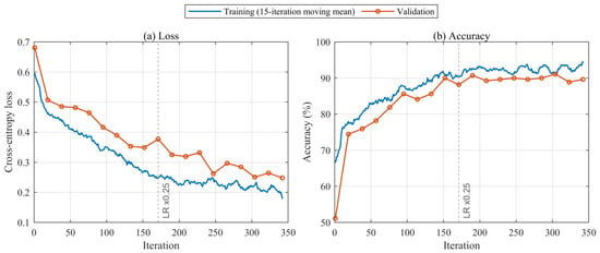
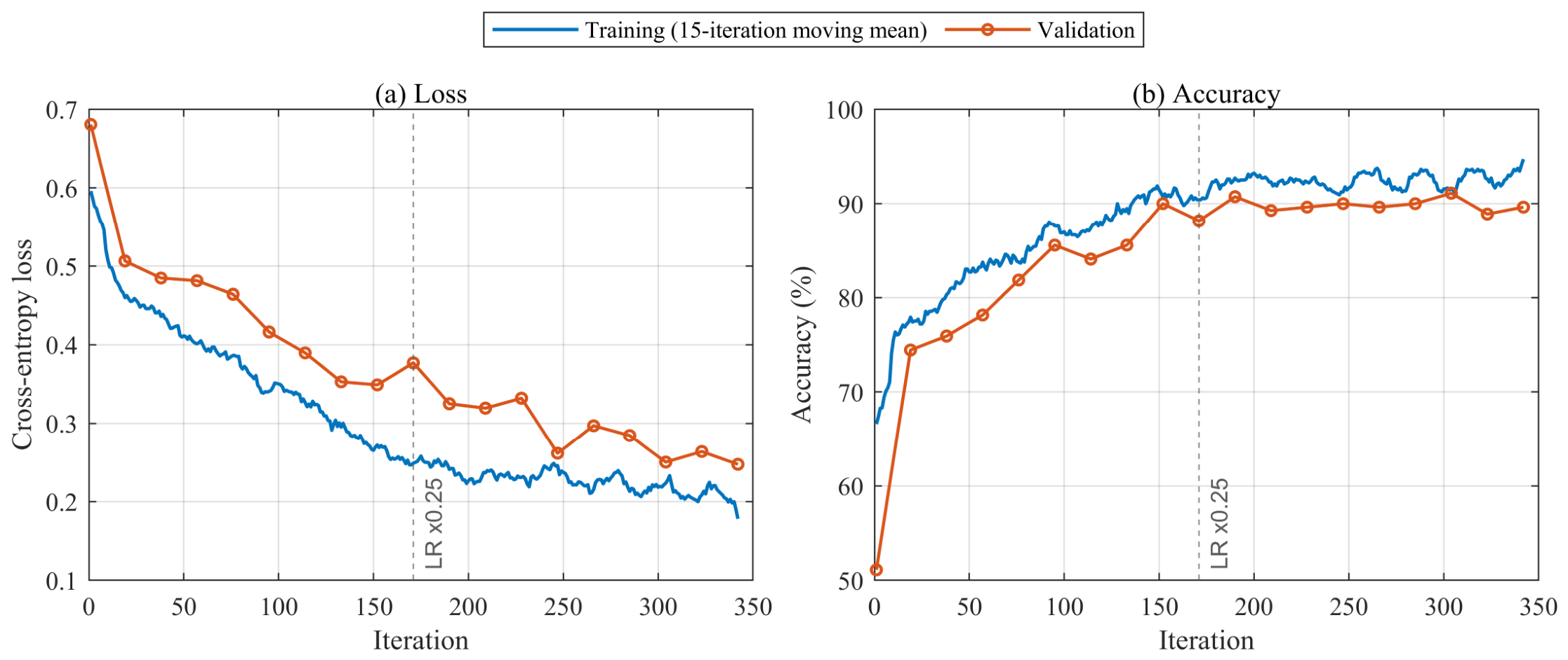
The training curves in Figure 5 show a rapid initial decrease in cross-entropy and a slower refinement after approximately 100 iterations. The blue trace is a 15-iteration moving mean of minibatch values, whereas the validation points are recorded once per validation interval; the vertical marker indicates the epoch 9 learning-rate reduction. At the last recorded validation point, the smoothed training accuracy is 92.92% and validation accuracy is 89.63%, a gap of approximately 3.29 percentage points. This modest train-validation gap is consistent with mild overfitting in the fixed-seed run and reinforces the need for the independent-seed analysis rather than serving as evidence of convergence by itself.

Figure 5. Fixed-seed CNN optimization history: (a) cross-entropy loss; (b) accuracy. Training traces use a 15-iteration moving mean, validation values are shown only at their recorded intervals, and the dashed line marks the learning-rate reduction after epoch 9. The final displayed smoothed training-versus-validation accuracy gap is approximately 3.29 percentage points.

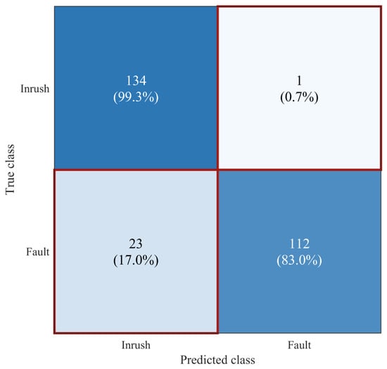
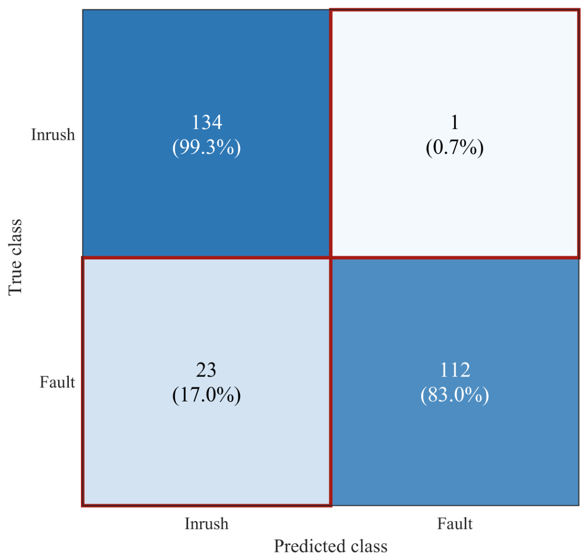
On the independent 270-record test set, the CNN correctly classified 134 of 135 inrush records and 112 of 135 fault records. The resulting accuracy was 91.11%, inrush precision 85.35%, inrush recall 99.26%, F1 score 91.78%, specificity 82.96%, and AUC 0.9833. The 23 false-positive fault records show that randomizing event onset removes the near-perfect alignment shortcut but leaves a nontrivial overlap between late fault records and truncated inrush records. In the protection terminology used here, security means avoiding an unwanted trip during magnetizing inrush, whereas dependability means issuing a trip for an actual internal fault. The error pattern therefore favors security through high inrush recall but reduces dependability through fault-to-inrush errors; threshold selection should consider both quantities rather than accuracy alone. The class-by-class counts are shown in Figure 6.

Figure 6. Confusion matrix for the proposed 1D CNN on the independent 270-record test set (135 records per class). Inrush is listed first; percentages are normalized within each true class. The shade of blue indicates the proportion of samples in each cell, with darker blue corresponding to a higher proportion. Off-diagonal cells are marked with red borders so the 0.7% and 17.0% error rates remain visually distinct from the correct classifications.

The fixed-seed confusion matrix also illustrates why precision and recall should be read together. The CNN misses only one inrush record, so a protection logic that uses the inrush probability for temporary blocking would rarely expose an inrush case as an internal fault in this realization. However, 23 fault records are assigned to inrush, which lowers specificity and precision. These false positives are not interchangeable: a fault with a late onset, low amplitude, or strong CT clipping may be more difficult to distinguish than a large fault immediately after the window begins. The model output should therefore be combined with a relay’s existing differential current and restraint logic, and the cost of a delayed trip should be evaluated explicitly in a field-oriented threshold study.

The ROC curve separates ranking quality from a single operating threshold. The CNN AUC of 0.9833 indicates that its probability ranking is strong for the fixed test set even though the default maximum-probability decision produces false positives. A relay could choose a different threshold to increase fault specificity at the expense of inrush recall, or it could use a two-stage rule in which low-confidence cases are held for an additional cycle. To avoid tuning on the test set, the decision threshold is selected on the validation set in Section 4.2; the default rule is reported here for comparison.

The prefix-occlusion control supports the alignment audit. Replacing the first 5 ms of every normalized test record by the training mean gives 90.74% accuracy, 98.52% inrush recall, and 0.9835 AUC; replacing the first 10 ms gives 89.63%, 96.30%, and 0.9698, respectively. The moderate rather than catastrophic change is consistent with the randomized-onset design: the CNN still uses the remaining pulse and fault morphology, while the first samples are not a deterministic class marker.

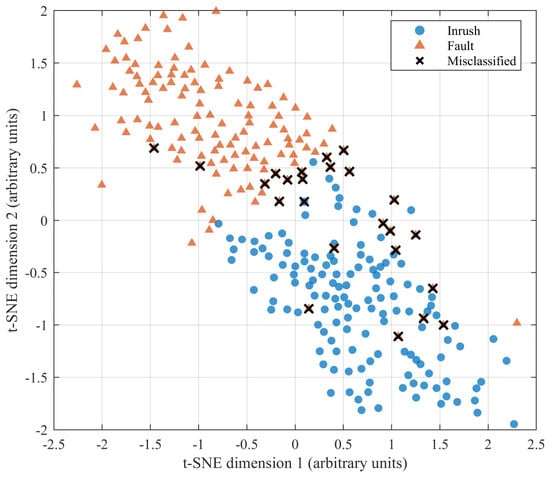
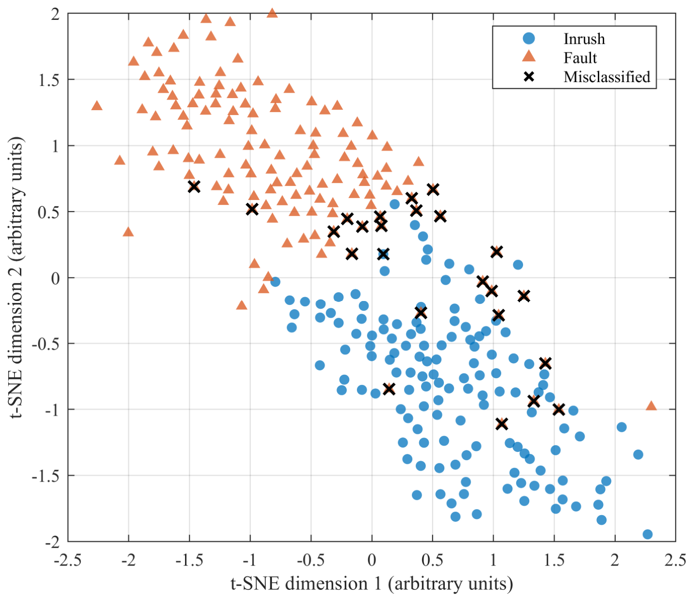
The projection in Figure 7 maps the 64 global-average-pooled features into two dimensions using t-SNE with perplexity 30, 100 print iterations, and random seed 20260920. The two classes form broad but overlapping regions rather than a perfectly empty transition band; the black crosses identify the 24 misclassified test records, comprising 23 internal-fault records predicted as inrush and one inrush record predicted as fault. Several inrush subgroups are visible, plausibly reflecting different onset locations, dominant limbs, and disturbance combinations. The coordinates are standardized arbitrary units and distances are not a statistical test of separability.

Figure 7. Descriptive t-SNE projection of the 64 CNN features for the independent test records. Perplexity = 30, NumPrint = 100, seed = 20260920; axes are arbitrary standardized units. Black crosses mark the 24 errors: 23 internal faults predicted as inrush and one inrush record predicted as fault.

The latent projection is used only as a descriptive diagnostic. t-SNE preserves selected neighborhood relations while distorting global distances, so the apparent size or separation of a cluster cannot be converted into a confidence interval or a physical distance between operating states. Its value here is to expose whether errors are scattered across the representation or concentrated near a transition region. The overlap visible in the projection is consistent with the engineering interpretation of the task: inrush and fault are not two perfectly disjoint signal classes after CT distortion, random onset, noise, and parameter variation are introduced.

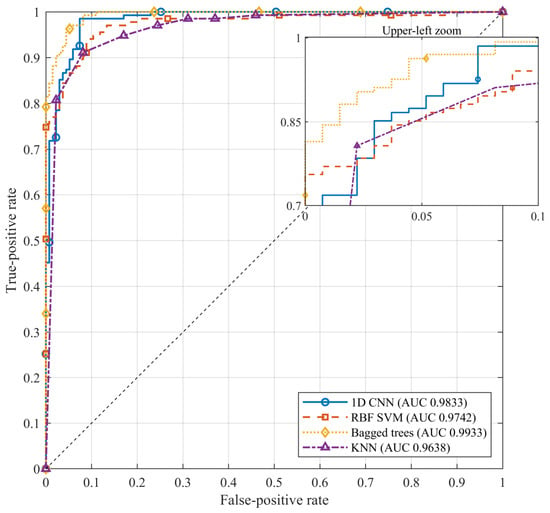
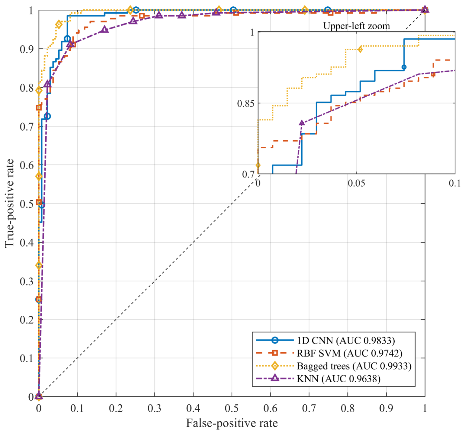
The comparison in Table 5 uses the CNN and three classifiers trained on the compact descriptor vector defined in Section 3.3. The onset-randomized data expose a clear trade-off: the bagged trees reach 95.56% accuracy and 0.9933 AUC, the RBF SVM reaches 92.22% and 0.9742 AUC, while the CNN reaches 91.11% and 0.9833 AUC. The CNN preserves the highest inrush recall among the four models (99.26%) and supplies a direct phase-time attribution path, whereas the tree and SVM models use engineered amplitude and harmonic summaries. These results do not establish universal superiority; they show that the sequence model remains competitive after the alignment shortcut is removed and that its interpretability is a distinct design objective. Figure 8 gives the corresponding ROC comparison with four-decimal AUC labels and an upper-left inset.

Table 5. Independent test-set performance of the proposed CNN and baseline classifiers.

Model	Accuracy (%)	Precision (%)	Recall (%)	F1 (%)	AUC
1D CNN	91.11	85.35	99.26	91.78	0.9833
RBF SVM	92.22	90.71	94.07	92.36	0.9742
Bagged trees	95.56	94.24	97.04	95.62	0.9933
KNN	86.30	79.88	97.04	87.63	0.9638

Precision, recall, and F1 treat magnetizing inrush as the positive class. The high values apply to the synthetic model family and do not establish field generalization.

Figure 8. Receiver-operating-characteristic curves for the CNN and traditional machine learning baselines. AUC values are printed to four decimals; distinct line styles and markers identify the four models, and the inset enlarges the upper-left operating region.

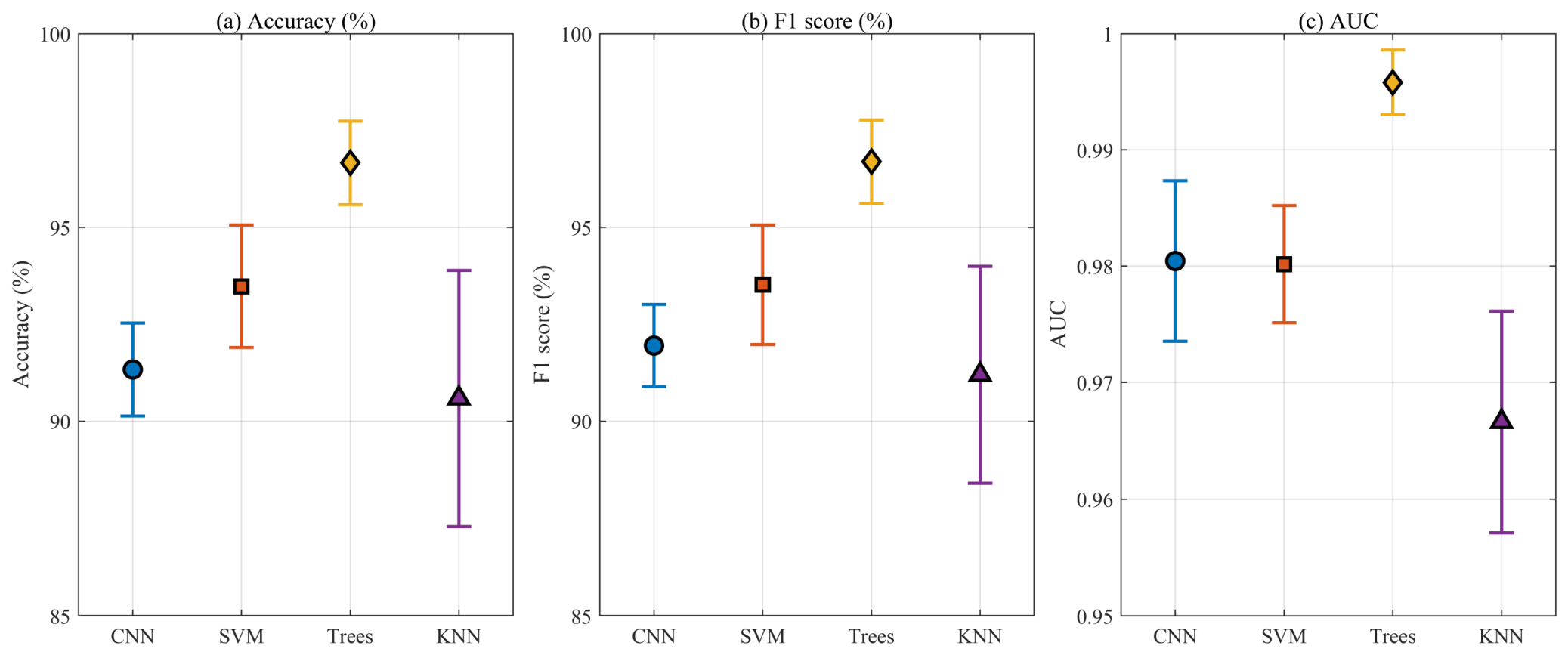
The nominal ranking is stable when the complete experiment is regenerated with five independent seeds, although the baseline models remain stronger on several aggregate measures. The CNN accuracy is 91.33% ± 0.97% and its AUC is 0.9804 ± 0.0056; the bagged-tree ensemble reaches 96.67% ± 0.87% accuracy and 0.9958 ± 0.0022 AUC. The SVM averages 93.48% ± 1.27% accuracy, while KNN has the largest accuracy spread at 90.59% ± 2.65%. The CNN’s inrush recall is 98.96% ± 0.66%, higher than the SVM mean of 94.07% ± 1.17% and comparable to the tree mean of 97.63% ± 1.42%. Thus the direct-sequence model is not the best nominal classifier in this simulator, but it offers high inrush recall, a compact architecture, and a physically indexed attribution mechanism.

Because the study is motivated by the limitations of second-harmonic and waveform-based rules, the first comparison evaluates these fixed criteria on the same independent test set. For each phase, the second-harmonic ratio is the ratio of spectral magnitude in the 90–110 Hz band to that in the 45–55 Hz band, and the criterion blocks tripping when the largest phase ratio exceeds 0.15. The dead-angle rule estimates the fraction of one cycle spent below 5% of the peak and blocks when it exceeds 60°. Table 6 shows that neither fixed rule is robust on this stress-tested benchmark. The second-harmonic threshold blocks 124 of 135 internal faults (specificity 8.15%) because the decaying-DC offset and wideband distortion of short fault windows leak into the second-harmonic band, whereas the dead-angle rule instead misses 119 of 135 inrush records (recall 11.85%). Combining the two rules does not resolve this failure because their operating points move in opposite directions. This is not a statement that these rules fail in every relay, where longer data windows and adaptive thresholds are used; it shows that fixed thresholds become brittle on the diverse, randomized, and CT-distorted windows used here, which is the motivation for a learned classifier.

Table 6. Fixed second-harmonic and dead-angle criteria on the independent test set.

Rule	Accuracy (%)	Precision (%)	Inrush Recall (%)	Specificity (%)	F1 (%)	Faults Blocked	Inrush Missed
Second-harmonic restraint (ratio > 0.15)	50.00	50.00	91.85	8.15	64.75	124	11
Dead-angle criterion (>60 deg)	55.56	94.12	11.85	99.26	21.05	1	119
Combined harmonic/dead-angle	50.00	50.00	91.85	8.15	64.75	124	11

To answer the Introduction question of whether an image transformation or a recurrent module is needed for a short three-phase window, two alternative networks are trained on the same partitions and labels with comparable training budgets. The LSTM feeds the normalized sequence into a 48-unit recurrent layer followed by 20% dropout and the same two-node softmax classifier. The GASF CNN converts each window to a 40 × 40 Gramian-angular-summation-field image per phase and trains a three-block image CNN. Table 7 shows that the LSTM and the direct 1D CNN reach the same accuracy (91.11%), with the direct CNN having the highest inrush recall (99.26%) and the LSTM a higher specificity (84.44%). The GASF-image CNN reaches the highest accuracy (94.81%) and specificity (94.07%), but its inrush recall is lower (95.56%), it requires an image-encoding stage, and it carries more parameters; its advantage is therefore a different security/dependability trade-off rather than domination. The comparison is controlled rather than exhaustive—each architecture uses the same labels and validation protocol. It answers the Introduction question directly: for a short three-phase window, an image transform or recurrent module is not necessary to attain the best inrush recall, while the image formulation offers a modest accuracy gain at the cost of recall and added complexity.

Table 7. Direct 1D CNN versus recurrent LSTM and GASF-image CNN.

Model	Accuracy (%)	Precision (%)	Inrush Recall (%)	Specificity (%)	F1 (%)	AUC
1D CNN (proposed)	91.11	85.35	99.26	82.96	91.78	0.9833
LSTM	91.11	86.27	97.78	84.44	91.67	0.9369
GASF-image CNN	94.81	94.16	95.56	94.07	94.85	0.9925

4.2. Threshold Selection and Robustness Analysis

The classifiers above use the default maximum-probability rule, which corresponds to a decision threshold of 0.5 on the inrush probability and yields 23 internal faults classified as inrush; in a relay this would block tripping during a genuine fault and is a loss of dependability. The operating threshold should therefore not be chosen on the test set. It is instead selected on the validation set to maximize balanced accuracy (the mean of inrush recall and fault specificity) and then applied once to the test set. Table 8 shows that the validation-selected threshold (0.655) reduces the faults classified as inrush from 23 to 12 (8.9% of faults) and raises accuracy to 94.81% and specificity to 91.11%, while inrush recall changes only from 99.26% to 98.52%. The trade-off is made explicit: the threshold is a protection setting rather than a property of the network, and a deployment relay could combine it with restraint currents and a blocking timer.

Table 8. Default versus validation-selected decision threshold.

Threshold	Accuracy (%)	Inrush Recall (%)	Specificity (%)	F1 (%)	Faults Blocked	Inrush Missed
Default 0.500	91.11	99.26	82.96	91.78	23	1
Validation-selected 0.655	94.81	98.52	91.11	95.00	12	2

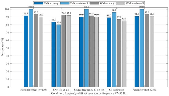
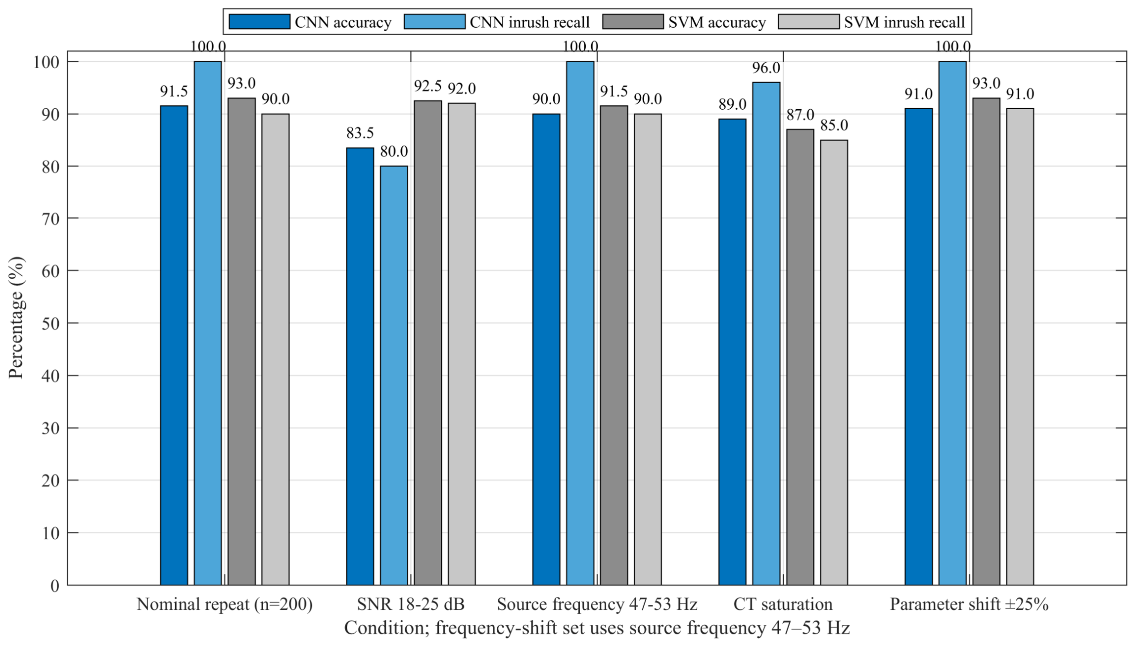
In the robustness comparison, Figure 9 and Table 9 summarize one nominal repeat and four out-of-distribution sets, each containing 100 inrush and 100 fault records. The nominal repeat is a newly generated 200-record set and is not the fixed 270-record test set used for Table 5. On the shifted sets, CNN accuracy is 83.5% at 18–25 dB SNR, 90.0% for a 47–53 Hz source-frequency shift, 89.0% with asymmetric CT saturation forced in both classes, and 91.0% under the ±25% parameter shift. Inrush recall falls to 80%, 100%, 96%, and 100%, respectively. The low-SNR condition is therefore the most demanding in this realization; the saturation set also reduces the inrush recall to 96%. These are single-seed, single-repeat estimates; the paper does not assign statistical significance to the differences.

Figure 9. Fixed-seed robustness results for the 1D CNN and RBF SVM on one nominal repeat and four shifted conditions. Every condition is an independently generated 200-record set containing 100 inrush and 100 fault records. Bars start at 0%; source-frequency shift denotes 47–53 Hz. These are seed-20260920 results, not the five-seed means reported in Section 4.2.

Table 9. Accuracy and inrush recall on independently generated robustness sets.

Condition	CNN Accuracy (%)	CNN Recall (%)	SVM Accuracy (%)	SVM Recall (%)
Nominal repeat (n = 200)	91.5	100	93.0	90
SNR 18–25 dB	83.5	80	92.5	92
Source frequency 47–53 Hz	90.0	100	91.5	90
CT saturation	89.0	96	87.0	85
Transformer-parameter shift ±25%	91.0	100	93.0	91

The five-seed robustness summary changes the emphasis slightly. The nominal-repeat accuracy is 92.1% ± 1.8% and the source-frequency-shift accuracy is 91.8% ± 2.1%, indicating that the CNN generally preserves its ranking when the frequency moves within the tested band. The low-SNR set is substantially harder, with 80.8% ± 3.3% accuracy and 74.2% ± 7.6% inrush recall. The wide recall standard deviation reflects the limited 200-record size of each repeat and the sensitivity of borderline cases to the regenerated noise realization. Forced CT saturation gives 88.1% ± 2.6% accuracy and 94.8% ± 2.4% recall, while the ±25% parameter shift gives 91.0% ± 1.9% accuracy and 99.6% ± 0.9% recall. These intervals describe repeated synthetic experiments; they do not quantify uncertainty over unobserved transformer designs.

The stress results suggest different mitigation priorities. Improving the noise front end, averaging several samples, or calibrating the probability under low SNR may be more valuable than adding a larger network. CT saturation should be treated as a joint primary-and-secondary phenomenon: a primary fault waveform can be continuous while the measured differential current becomes asymmetric and clipped. The current soft-tanh channel is a useful controlled perturbation, but future work should replace it with measured CT magnetization curves and remanence states. Likewise, a frequency shift alone is not a complete grid-disturbance model; voltage magnitude, phase-angle jumps, and frequency ramps should be varied together in a laboratory or EMT study.

To quantify stochastic variation, the complete MATLAB protocol was repeated for seeds 20260920, 20260921, 20260922, 20260923, and 20260924. Each run regenerated 1800 nominal records, performed a new 70:15:15 stratified split, initialized and trained a new CNN, fitted new baselines, and generated new 200-record robustness sets. No result from one seed was used to tune another seed. The statistic reported below is therefore a mean over five complete experiments, and the standard deviation includes variation in the synthetic records, partition, initialization, minibatch order, and robustness realization. It should not be interpreted as five independent transformers or as a field-level confidence interval.

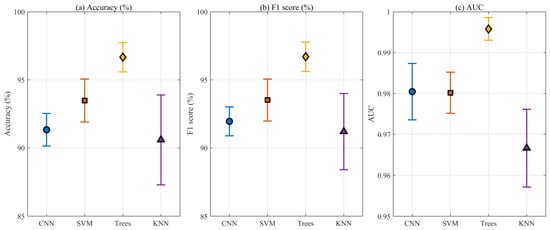
Figure 10 plots the mean and 95% confidence interval for accuracy, F1 score, and AUC. The CNN has a narrow accuracy interval (90.13–92.53%) and a high mean inrush recall of 98.96%, but the tree ensemble remains higher on nominal accuracy and AUC. KNN shows the largest spread, especially for specificity, which is consistent with a local-distance classifier operating on heterogeneous amplitude and harmonic descriptors. The confidence intervals are descriptive t-intervals over five seed-level observations; they are not a substitute for a hierarchical model over physical transformers, nor do they test statistical significance between methods. Detailed information can be found in Table 10.

Figure 10. Five-seed model statistics shown as point estimates with 95% t-intervals for (a) accuracy, (b) F1 score, and (c) AUC. The percentage panels use 85–100% and the AUC panel uses 0.95–1.00 so the uncertainty intervals remain legible; no bar baseline is implied. The intervals represent stochastic variation within the stated simulation protocol, not cross-transformer field uncertainty.

Table 10. Model performance across five independent random seeds.

Model	Accuracy (%)	Precision (%)	Recall (%)	Specificity (%)	F1 (%)	AUC
1D CNN	91.33 ± 0.97	85.87 ± 1.20	98.96 ± 0.66	83.70 ± 1.57	91.95 ± 0.86	0.9804 ± 0.0056
RBF SVM	93.48 ± 1.27	92.99 ± 1.66	94.07 ± 1.17	92.89 ± 1.78	93.52 ± 1.24	0.9802 ± 0.0040
Bagged trees	96.67 ± 0.87	95.79 ± 0.91	97.63 ± 1.42	95.70 ± 0.97	96.70 ± 0.87	0.9958 ± 0.0022
KNN	90.59 ± 2.65	86.08 ± 3.70	97.04 ± 0.74	84.15 ± 5.04	91.20 ± 2.25	0.9666 ± 0.0077

Values are mean ± standard deviation over seeds 20260920–20260924. The accompanying multiseed_model_summary.csv contains N, standard deviation, and 95% confidence limits for every metric.

Typical digital relays operate within roughly one to two cycles, so a 40 ms window is not the only relevant choice. The same CNN and protocol are trained on windows of 10, 20, and 30 ms, with event onsets randomized independently within each window. Table 11 shows that the network retains competitive accuracy on the shorter windows (90.00% at 10 ms and 93.33% at 20–30 ms), with specificity comparable to the 40 ms result. The slightly higher accuracy on 20–30 ms windows is consistent with one to one-and-a-half cycles concentrating the discriminating morphology. These single-seed results indicate that the learned features are not specific to a 40 ms window and remain usable within typical relay operating times; the absolute values should still be confirmed with the five-seed and field protocols.

Table 11. CNN performance on shorter analysis windows.

Window	Accuracy (%)	Precision (%)	Inrush Recall (%)	Specificity (%)	F1 (%)	AUC
40 ms window	91.11	85.35	99.26	82.96	91.78	0.9833
10 ms window	90.00	84.62	97.78	82.22	90.72	0.9589
20 ms window	93.33	88.24	100.00	86.67	93.75	0.9879
30 ms window	93.33	88.74	99.26	87.41	93.71	0.9673

4.3. Architecture Selection and SHAP Interpretation

The architecture is sometimes presented as if its depth, width, and kernel sizes were arbitrary, so an ablation retrains the network under five controlled variations. Table 12 shows that removing the third convolutional block (78.89%) or narrowing the channels to 8/16/32 (81.85%) materially lowers accuracy, and replacing the 9/5/3 kernels by uniform three-sample kernels (84.07%) or removing dropout (87.78%) also degrades it. A wider 32/64/128 network reaches 92.59% on this single seed, about 1.5 percentage points above the final design, but this is within the run-to-run variation (about one percentage point standard deviation) and it roughly quadruples the parameters and the opportunity to memorize the synthetic generator. The final three-block, 16/32/64, 9/5/3 design is therefore the best measured accuracy-to-size trade-off: simpler variants are clearly worse, while over-parameterization gives no reliable benefit. The larger kernels were retained because, at 8 kHz, the nine-sample kernel spans 1.125 ms and captures pulse width directly, whereas uniform three-sample kernels must assemble the same width through several layers.

Table 12. Architecture-selection ablation on the fixed-seed test set.

Variant	Accuracy (%)	Precision (%)	Inrush Recall (%)	Specificity (%)	F1 (%)	AUC
Final (3 blocks, 16/32/64, k 9/5/3)	91.11	85.35	99.26	82.96	91.78	0.9833
Two blocks (16/32, k 9/5)	78.89	70.97	97.78	60.00	82.24	0.8894
Narrow (8/16/32)	81.85	74.71	96.30	67.41	84.14	0.9306
Wide (32/64/128)	92.59	87.58	99.26	85.93	93.06	0.9934
Uniform kernels (k 3/3/3)	84.07	76.14	99.26	68.89	86.17	0.9503
No dropout	87.78	80.72	99.26	76.30	89.04	0.9717

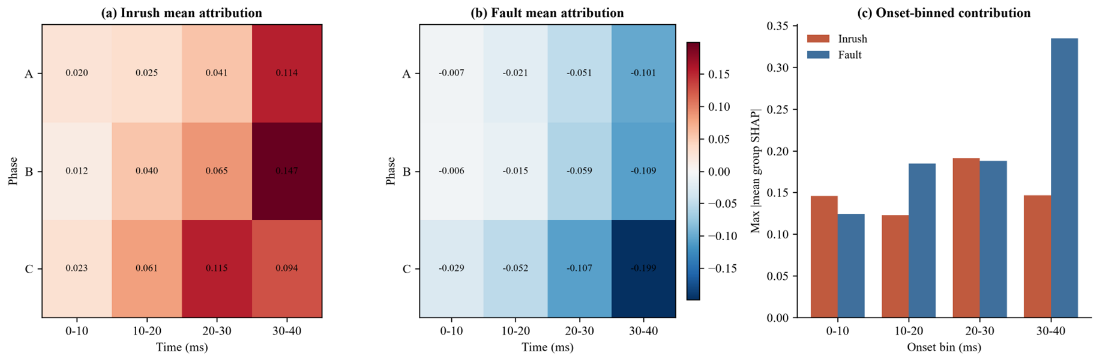
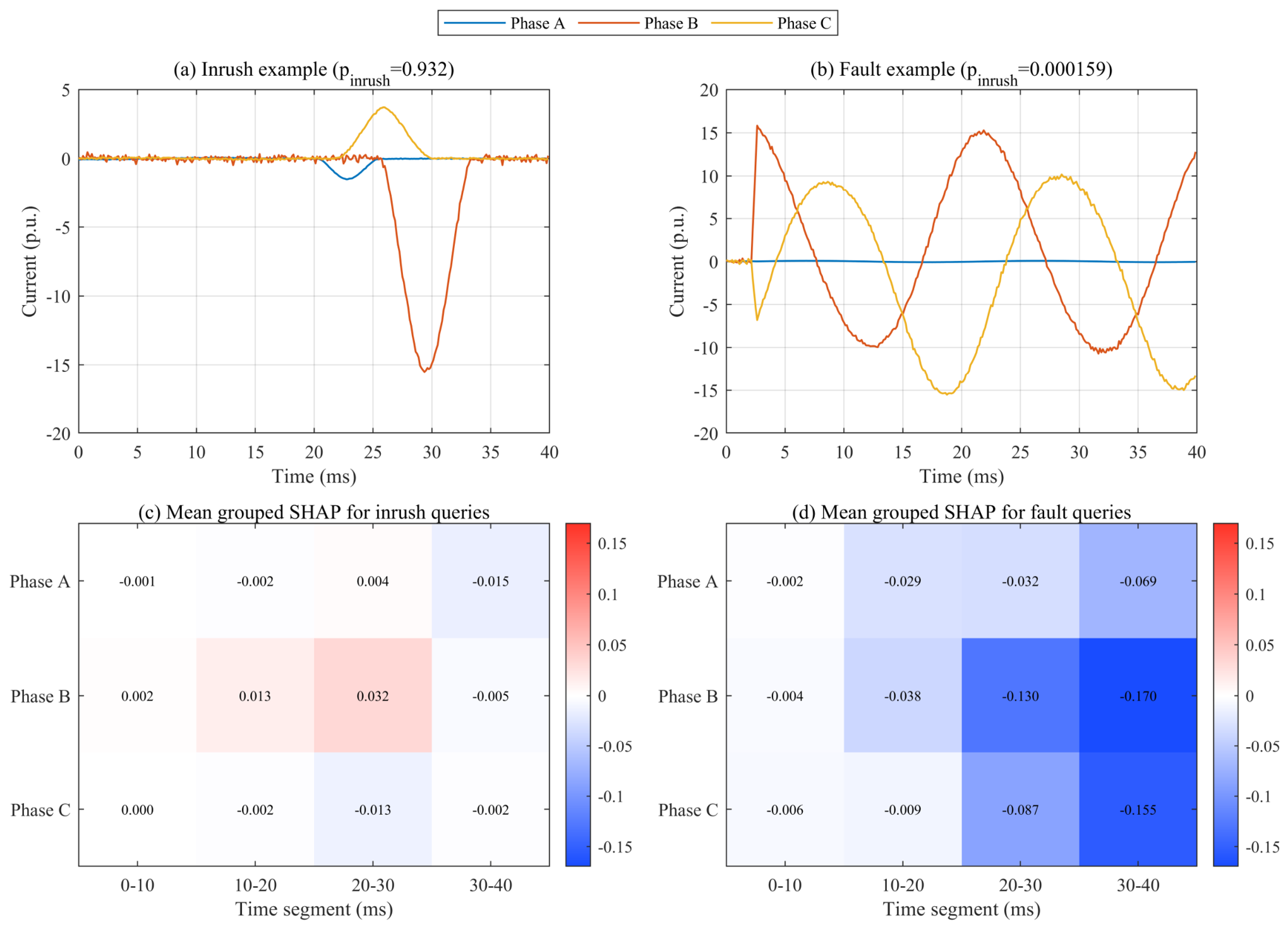
The representative examples are now complemented by the population analysis in Figure 11, which addresses the limitations of averaging only six samples against a single median. Exact grouped SHAP was recomputed for every correctly classified test record (134 inrush and 112 fault records) using a ten-record background set from the opposite class, so the base value is the mean model output over realistic records rather than a single median waveform. The population mean attributions are shown for inrush (Figure 11a) and faults (Figure 11b): the inrush mean is positive and concentrated in the later time groups, with the largest values in the 20–40 ms bins (0.114–0.147), while the fault mean is negative throughout and stronger in magnitude, with the last 10 ms of phases A, B, and C at −0.101, −0.109, and −0.199. The fault direction is therefore the larger and more consistent population-level signal. Binning the same records by onset position (Figure 11c) controls the previously unpaired onset effect: inrush contributions stay within 0.12–0.19 across bins, whereas the fault contribution grows for late-onset records (0.335 in the 30– 40 ms bin), so the fault signal is not a single-boundary artifact but the later bins are still the most informative. For the matched inrush and fault examples in Figure 12, the inrush probability changes from 0.8894 to 0.9325 and from 0.9012 to 0.000159, respectively, with a maximum efficiency residual of 5.2 × 10⁻⁷.

Figure 11. Population exact grouped SHAP over all correctly classified test records. Rows denote the three phases (A, B, C), and columns denote 10 ms onset bins (0–10, 10–20, 20–30, and 30–40 ms); each heat-map cell corresponds to one phase and one 10 ms interval. (a) Mean signed attribution for inrush; (b) mean signed attribution for faults; and (c) onset-binned mean absolute contribution. In (a,b), red indicates positive signed SHAP values that push the prediction toward inrush, blue indicates negative values that push the prediction toward fault, and near-white cells indicate values close to zero, with the color scale ranging from −0.15 to +0.15. In (c), the red and blue bars denote inrush and fault, respectively, and the vertical axis reports the maximum mean absolute group SHAP value in each onset bin.

Figure 12. Matched representative and six-sample exact grouped SHAP attribution. (a,b) Matched representative waveforms with their CNN inrush probabilities and an external three-phase legend. (c) Mean signed attribution over six correctly classified inrush queries. (d) Mean signed attribution over six correctly classified fault queries. Each cell corresponds to one phase and one 10 ms segment; red supports the inrush class and blue supports the fault class relative to an opposite-class median background, and the printed values are the mean SHAP contributions.

The Figure 12 presents the SHAP attribution analysis based on matched representative samples and an exact six-sample grouped design. Subplots (a) and (b) show the matched representative waveforms, along with their corresponding CNN-calculated inrush probabilities and an external three-phase legend. Subplot (c) depicts the mean signed attribution across six correctly classified inrush queries, and Subplot (d) depicts the mean signed attribution across six correctly classified fault queries. Each cell in the attribution maps corresponds to one phase and one 10-ms time segment; red shading indicates features that support the inrush class, blue shading indicates features that support the fault class (both benchmarked against the median background of the opposite class), and the printed numerical values represent the mean SHAP contributions.

Together, the population and onset-binned analyses support a cautious statement: exact grouped SHAP provides reproducible, numerically exact, phase-time attribution over the complete correctly classified test set, with a consistent negative fault direction concentrated in the later time groups. The heat-map values are signed contributions to the inrush probability: red supports inrush relative to the multi-record background and blue supports fault, with cell values printed so weak phase contributions are not overstated by color. The remaining limitation is physical rather than numerical: the attribution identifies what the CNN uses within this model family, not a universal relay criterion, and the concentration of signal in the later bins partly reflects the randomized onset leaving less event content in the earliest bins. It must therefore be re-checked on cross-transformer and field records.

4.4. Scope and Limitations

The study is a simulation-based method paper. The inrush generator uses a reduced single-valued magnetic backbone, an idealized three-limb zero-sum constraint, and no explicit minor-loop or frequency-dependent core-loss model. The fault and CT channels are parameterized signal models rather than electromagnetic transient models of a specific protection installation. The 117 operating-point files and four-case peak check support internal consistency and parameter-range selection, but they do not replace synchronized field recordings or laboratory switching tests. The 50 kHz-to-8 kHz resampling path also omits an explicit anti-alias filter, which should be revisited in a measurement-grade implementation.

A second limitation is the absence of transformer-level grouping across different physical units. Although the robustness sets shift parameters, every record comes from the same model family. The five-seed experiment now quantifies stochastic variation within that family, but it does not establish multi-transformer generalization or statistical significance under a deployment population. The onset-occlusion control reduces the alignment-leakage concern, but it does not rule out every simulator-specific shortcut. Future validation should train and test across measured records from different transformer ratings, vector groups, CT designs, fault inception angles, breaker pole scatter, and laboratory switching campaigns. Feature-transfer strategies such as [20], calibration, inference latency on relay-class hardware, and an uncertainty-aware trip/hold policy should be evaluated before protection deployment.

Several modeling details also limit the physical interpretation. The reduced backbone is single-valued and does not represent minor loops, hysteresis loss, eddy-current loss, temperature dependence, frequency-dependent permeability, or manufacturing variation. The source voltage contains selected harmonic terms rather than a measured distorted waveform. The fault generator uses analytical masks and decaying-DC components instead of a full EMT network with breaker pole scatter and frequency-dependent arc behavior. The CT channel is an asymmetric soft-saturation approximation without a measured excitation curve, remanence state, or burden-dependent recovery. These choices are appropriate for a transparent benchmark, but they can understate or misplace the difficult cases encountered by a field relay.

Finally, the current study evaluates an offline classification window. It does not implement a streaming buffer, a field-calibrated protection threshold, a trip/hold state machine, a communication delay, or a hardware-in-the-loop test. A 91% accuracy value cannot be translated directly into a relay failure rate because event frequencies, class costs, and clearing policies are different. The reproducible artifacts should therefore be used to compare modeling choices and identify informative phase-time evidence. Before deployment, the same code structure should be connected to field or laboratory recordings, with cross-transformer splits, pre-registered operating points, calibration curves, uncertainty monitoring, and an explicit analysis of the cost of false blocking versus false tripping.

5. Conclusions

A complete MATLAB R2023b pipeline was developed for transformer magnetizing-inrush identification with a compact 1D CNN and exact grouped SHAP analysis. The nonlinear three-limb inrush model reproduced four reference peak-current cases with less than 0.14% error after a single baseline current-base calibration. The 1800-record classification set included residual-flux variation, harmonic voltage, DC bias, four internal-fault types, noise, CT saturation, and independently randomized event onsets.

After removing the window-alignment shortcut, the CNN achieved 91.11% accuracy, 99.26% inrush recall, 91.78% F1 score, and 0.9833 AUC on the independent test set; selecting the decision threshold on the validation set raised accuracy to 94.81% and specificity to 91.11% while retaining 98.52% inrush recall. Across five independent seeds, the corresponding means were 91.33% ± 0.97% accuracy, 98.96% ± 0.66% inrush recall, 91.95% ± 0.86% F1, and 0.9804 ± 0.0056 AUC. Accuracy on the nominal repeat and four shifted sets averaged 92.1%, 80.8%, 91.8%, 88.1%, and 91.0%, respectively, with low-SNR inrush recall averaging 74.2%. The compact direct-sequence model matched an LSTM and retained the highest inrush recall, while an image CNN gained specificity at the cost of recall; the CNN retained competitive performance on 10–20 ms windows, whereas fixed second-harmonic and dead-angle criteria were brittle on the stress-tested benchmark. Bagged trees and the RBF SVM were stronger on some nominal metrics, so the evidence supports the CNN primarily for direct-sequence learning and phase-time interpretability rather than an unconditional accuracy advantage.

Exact grouped SHAP was recomputed over all correctly classified test records with a multi-record opposite-class background, and the same records were paired within onset bins; the 5/10 ms prefix-occlusion check, the manifest-level onset audit, and the repeated-seed results provide progressively stronger checks against a single-window artifact, but none establishes field generalization. The method should therefore be advanced with field recordings, cross-transformer feature transfer, calibrated relay thresholds, and hardware-in-the-loop testing before it supports a protection decision threshold.

References

- Specht, T.R. Transformer magnetizing inrush currents. Trans. AIEE 1951, 70, 323–327. [Google Scholar] [CrossRef] [Scilit]
- Holcomb, J.E. Distribution transformer magnetizing inrush current. Trans. AIEE Part III Power Appar. Syst. 1961, 80, 697–702. [Google Scholar] [CrossRef] [Scilit]
- Chiesa, N.; Mork, B.A.; Hoidalen, H.K. Transformer model for inrush current calculations: Simulations, measurements and sensitivity analysis. IEEE Trans. Power Deliv. 2010, 25, 2599–2608. [Google Scholar] [CrossRef] [Scilit]
- Yacamini, R.; Bronzeado, H. Transformer inrush calculations using a coupled electromagnetic model. IEE Proc. Sci. Meas. Technol. 1994, 141, 491–498. [Google Scholar] [CrossRef] [Scilit]
- Phadke, A.G.; Thorp, J.S. A new computer-based flux-restrained current-differential relay for power transformer protection. IEEE Trans. Power Appar. Syst. 1983, PAS-102, 3624–3629. [Google Scholar] [CrossRef] [Scilit]
- Zhang, A.Q.; Ji, T.Y.; Li, M.S.; Wu, Q.H.; Zhang, L.L. An identification method based on mathematical morphology for sympathetic inrush. IEEE Trans. Power Deliv. 2018, 33, 12–21. [Google Scholar] [CrossRef]
- Brunke, J.H.; Froehlich, K.J. Elimination of transformer inrush currents by controlled switching-Part I: Theoretical considerations. IEEE Trans. Power Deliv. 2001, 16, 276–280. [Google Scholar] [CrossRef] [Scilit]
- Perez, L.G.; Flechsig, A.J.; Meador, J.L.; Obradovic, Z. Training an artificial neural network to discriminate between magnetizing inrush and internal faults. IEEE Trans. Power Deliv. 1994, 9, 434–441. [Google Scholar] [CrossRef] [Scilit]
- Mao, P.L.; Aggarwal, R.K. A novel approach to the classification of the transient phenomena in power transformers using combined wavelet transform and neural network. IEEE Trans. Power Deliv. 2001, 16, 654–660. [Google Scholar] [CrossRef] [Scilit]
- Ma, J.; Wang, Z.; Yang, Q.; Liu, Y. A two-terminal network-based method for discrimination between internal faults and inrush currents. IEEE Trans. Power Deliv. 2010, 25, 1599–1605. [Google Scholar] [CrossRef] [Scilit]
- Shah, A.M.; Bhalja, B.R. Discrimination between internal faults and other disturbances in transformer using the support vector machine-based protection scheme. IEEE Trans. Power Deliv. 2013, 28, 1508–1515. [Google Scholar] [CrossRef] [Scilit]
- Bagheri, S.; Moravej, Z.; Gharehpetian, G.B. Classification and discrimination among winding mechanical defects, internal and external electrical faults, and inrush current of transformer. IEEE Trans. Ind. Inform. 2018, 14, 484–493. [Google Scholar] [CrossRef] [Scilit]
- Tripathy, M.; Maheshwari, R.P.; Verma, H.K. Power transformer differential protection based on optimal probabilistic neural network. IEEE Trans. Power Deliv. 2010, 25, 102–112. [Google Scholar] [CrossRef] [Scilit]
- Afrasiabi, S.; Afrasiabi, M.; Parang, B.; Mohammadi, M. Integration of accelerated deep neural network into power transformer differential protection. IEEE Trans. Ind. Inform. 2020, 16, 865–876. [Google Scholar] [CrossRef] [Scilit]
- Afrasiabi, S.; Afrasiabi, M.; Parang, B.; Mohammadi, M. Designing a composite deep learning based differential protection scheme of power transformers. Appl. Soft Comput. 2020, 87, 105975. [Google Scholar] [CrossRef] [Scilit]
- Afrasiabi, S.; Afrasiabi, M.; Parang, B.; Mohammadi, M.; Samet, H.; Dragicevic, T. Fast GRNN-based method for distinguishing inrush currents in power transformers. IEEE Trans. Ind. Electron. 2022, 69, 8501–8512. [Google Scholar] [CrossRef] [Scilit]
- Li, Z.; Jiao, Z.; He, A.; Xu, N. A denoising-classification neural network for power transformer protection. Prot. Control Mod. Power Syst. 2022, 7, 52. [Google Scholar] [CrossRef] [Scilit]
- He, A.; Jiao, Z.; Li, Z.; Liang, Y. Discrimination between internal faults and inrush currents in power transformers based on the discriminative-feature-focused CNN. Electr. Power Syst. Res. 2023, 223, 109701. [Google Scholar] [CrossRef] [Scilit]
- Raichura, M.B.; Patel, N.C. Review of methodologies used for detection of magnetising inrush and fault conditions in power transformer. IET Energy Syst. Integr. 2021, 3, 230–246. [Google Scholar] [CrossRef] [Scilit]
- Li, Z.; He, A.; Wang, X.; Chen, X.; Jiao, Z.; Xu, N.; Cui, Y. Discrimination between faults and inrush currents using a feature transfer strategy-based CNN for power transformers. IEEE Trans. Instrum. Meas. 2025, 74, 1–15. [Google Scholar] [CrossRef] [Scilit]
- Kiranyaz, S.; Ince, T.; Gabbouj, M. 1D convolutional neural networks and applications: A survey. Mech. Syst. Signal Process. 2021, 151, 107398. [Google Scholar] [CrossRef] [Scilit]
- LeCun, Y.; Bottou, L.; Bengio, Y.; Haffner, P. Gradient-based learning applied to document recognition. Proc. IEEE 1998, 86, 2278–2324. [Google Scholar] [CrossRef] [Scilit]
- Krizhevsky, A.; Sutskever, I.; Hinton, G.E. ImageNet classification with deep convolutional neural networks. Adv. Neural Inf. Process. Syst. 2012, 25, 1097–1105. [Google Scholar]
- Lundberg, S.M.; Lee, S.-I. A unified approach to interpreting model predictions. Adv. Neural Inf. Process. Syst. 2017, 30, 4765–4774. [Google Scholar]
- Lundberg, S.M.; Erion, G.; Chen, H.; DeGrave, A.; Prutkin, J.M.; Nair, B.; Katz, R.; Himmelfarb, J.; Bansal, N.; Lee, S.I. From local explanations to global understanding with explainable AI for trees. Nat. Mach. Intell. 2020, 2, 56–67. [Google Scholar] [CrossRef] [Scilit] [PubMed]
Disclaimer/Publisher’s Note: The statements, opinions and data contained in all publications are solely those of the individual author(s) and contributor(s) and not of MDPI and/or the editor(s). MDPI and/or the editor(s) disclaim responsibility for any injury to people or property resulting from any ideas, methods, instructions or products referred to in the content. |
© 2026 by the authors. Licensee MDPI, Basel, Switzerland. This article is an open access article distributed under the terms and conditions of the Creative Commons Attribution (CC BY) license.