Efficiency Analysis of Predictive Current Control in Multiphase Drives: A Comparison of Weighting Factor Elimination and Scheduling Methods

Abstract

Multiphase drives are of interest in transportation applications such as electric propulsion, where energy efficiency has a direct impact on range and on the feasibility of extended missions. Efficiency can be improved during the design phase, but for a given hardware platform, further gains must come from the control of the electrical drive. In this context, this paper addresses the issue of weighting factor elimination versus weighting factor selection in predictive stator current control of multiphase drives, where three cost function designs are compared. The first is a conventional formulation with a single weighting factor selected offline and held constant at all operating points. The second is a ranking-based scheme inspired by the Technique for Order of Preference by Similarity to Ideal Solution, in which the cost function terms are treated as separate targets and the candidate control action is selected from the aggregated classification, so that no weighting factor is required. The third retains the structure of the first, but this factor is programmed with the operating point using values obtained offline from the minimization of a meta cost function that combines multiple objectives. Experimental tests are conducted on a five-phase induction motor to assess and compare the performance of the three methods. The results show that no constant weighting factor performs well over the entire operating range, and that the ranking-based scheme, although it removes the weighting factor, still yields a fixed compromise. Scheduling the weighting factor with the operating point instead reduces the tracking error and the switching frequency simultaneously over most of the tested range, and hence the switching losses, which no constant value can achieve.

1. Introduction

Model Predictive Control (MPC) originated in the 1970s as a control strategy for complex processes, particularly those characterized by slow dynamics [1]. MPC uses a mathematical model of the system to predict its future behavior. Based on these predictions, the controller determines the control actions necessary for the system to achieve specific objectives by minimizing a cost function (CF) that quantifies the deviations between the system variables and their respective setpoints. Additional terms can be included in the CF to address secondary objectives, such as reducing control effort or limiting the variability of the control signals, while system and actuator constraints can be explicitly considered.

At each sampling instant, the optimization problem is solved using the current system state, but only the first control action of the optimal sequence is applied. The prediction horizon is then shifted forward and the optimization is repeated with updated measurements, following the receding horizon principle [2]. Despite its flexibility and ability to anticipate future system behavior, the repeated online optimization can impose a significant computational burden, limiting the use of MPC in systems with constrained computational resources or demanding response time requirements.

Advances in computing devices enabled the use of MPC for fast processes such as electric drives [3]. In this realm, a technique known as Finite State MPC (FSMPC) is a particular MPC variant that controls directly the states of the Voltage Source Inverter (VSI), achieving high bandwidth [4] at the cost of increased harmonic content [5,6] and non-uniform switching frequency [7,8]. FSMPC has been applied to many systems based on power converters, in particular to electrical drives. One particular application is found in traction/propulsion of different kinds of vehicles including the more electric aircraft [9]. Therefore, research in the most important academic databases highlights that multiphase electric drives are vital for electric aircraft propulsion [10,11] mainly due to their intrinsic properties: improved fault tolerance [12], the greater power density and enhanced phase power distribution [13,14], reduced DC-link harmonic [15], and lower torque oscillations [16].

The application of FSMPC to multiphase drives (MPD) has been favored by its adaptability and flexibility to support new topologies [17] and modulation techniques. In particular, the cost function can incorporate different primary and secondary objectives of interest in MPD, such as: $\alpha -\beta$ current tracking, $x-y$ current minimization, and VSI switching reduction [18]. These have an effect on overall drive efficiency [19], which in turn can enhance the aircraft range for a given battery charge [20]. Weighting Factors (WFs) are required for the different terms included in the CF. These are not only adequate the different magnitudes of the terms, but also provide relative importance to the terms in the optimization. Selecting the most adequate WF is a challenge [19]. This has prompted proposals regarding WF selection and WF elimination [21,22,23]. In this context, evolutionary optimization has been used in multi-objective problems such as controller tuning [24]. Multi-objective optimization avoids the aggregation of terms, unlike the CF approach, and enables working with each design objective individually. In addition, WF elimination has been proposed as a way to reduce the computational load of the optimization phase. Although recent proposals reduce said load for some particular cost functions [25], a general solution does not exist.

Different techniques for WF elimination have been applied to FSMPC of MPD. In particular, the open loop cancellation of $x-y$ currents using a multi-vector approach allows the elimination of the WF for said currents [26]. In a more general case, WF elimination can be achieved by Decision Making (DM) techniques that can accommodate different terms in the CF. Among the DM approaches, MPC combined with the Technique for Order Preference by Similarity to Ideal Solution (TOPSIS) method has emerged as a prominent strategy. These methods focus on addressing the primary control objectives, particularly in the context of Predictive Torque Control (PTC). For instance, in [27] a gray relational analysis for TOPSIS is applied to an Induction Motor (IM); similarly, in [28,29], the TOPSIS is applied to a surface-mounted permanent magnet synchronous motor. In [30], WF selection is carried out for a six-phase IM using a Multi-Objective Genetic Algorithm (MOGA). However, the $x-y$ subspace is not taken into account. In [31], a Non-dominated Sorting Genetic Algorithm II (NSGA-II) combined with TOPSIS is employed for PTC of a conventional IM. For MPD, operating-space partitioning has also been proposed to provide different WF tunings for different operating regions [32]. Online WF selection methods have also been investigated using various techniques, including neural networks [33], reinforcement learning [34], data-based entropy selection [35], and metaheuristic tuning [36].

An important aspect is that the conventional performance indicators exhibit trade-offs [37]. These relationships between figures of merit have been quantitatively characterized in [38]. Similar works do not exist for WF-free methods since the flexibility for WF tuning is lost. The existence of trade-offs must be taken into account for WF selection since it reduces the set of possible WF combinations to those in the Pareto front [39,40].

A preliminary, simulation-based analysis of the same cost-function design strategies for predictive current control of five-phase induction machines is presented in [41]. Here, however, the strategies are validated experimentally on a real test bench and assessed in terms of drive energy efficiency, which yields quantified and practical conclusions. First, an experimental comparison is carried out for three different CF design strategies for FSMPC. These are applied to a five-phase IM for electric aircraft propulsion. The first CF (S1 in what follows) is a conventional approach, using a single term that is selected offline and held constant for all operating points and it is included as a baseline for the comparison. The second CF (named S2) is a ranking-based scheme inspired by TOPSIS, where the terms are treated as separate targets and candidate control action is selected based on the aggregated classification. The third CF (S3) retains the structure of S1, but WFs are programmed with the operating point. This methodology requires the offline minimization of several conflicting criteria. To deal with this problem, in this work a meta CF is proposed. The meta CF balances current tracking error and the switching frequency. As a contribution, it can be stated that simply using a predictive control strategy and a multiphase drive in aircraft propulsion is insufficient. The energy efficiency of the system affects the inherent design of the control strategy. While S1 and S2 offer efficient results in specific operating ranges, losing performance in the rest of the spectrum, S3 maintained best balance across the tested range.

The article is organized as follows. Section 2 introduces the fundamentals of the predictive control algorithm applied to multiphase motors. Section 3 describes the experimental setup. Section 4 presents the experimental results, analyzes the main findings, and discusses their implications. Finally, Section 5 summarizes the main conclusions of the study.

2. Predictive Stator Current Control Algorithm

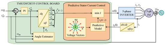
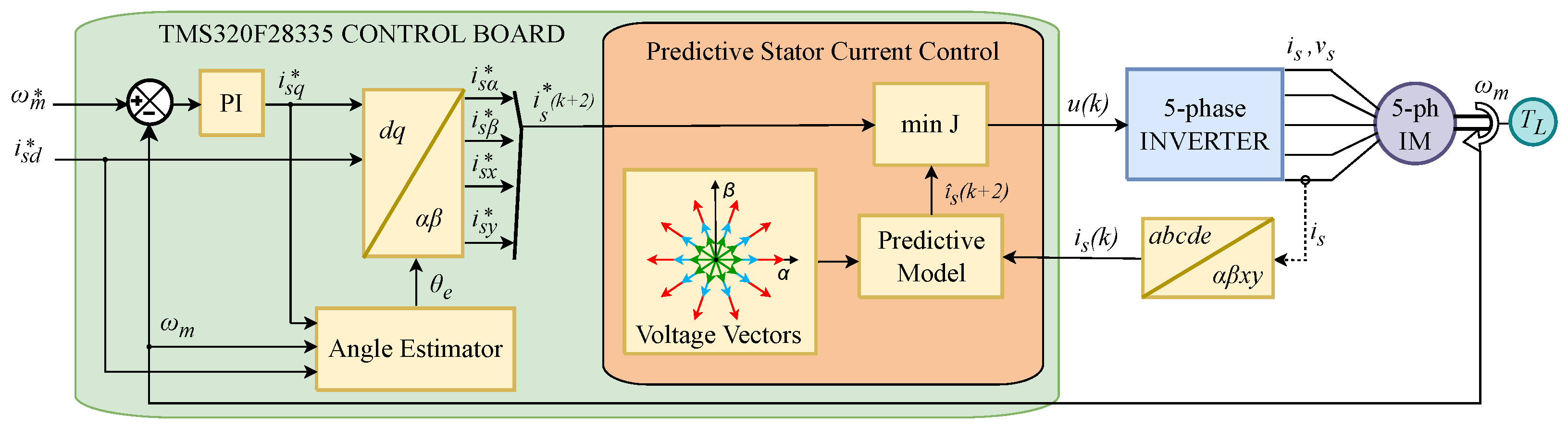
The block diagram of FSMPC of an electrical system using power converters is presented in Figure 1. It contains an algorithm that decides the control action u to be applied. It uses a program in which the tasks (waiting for next sample time, sampling, actuating) are sequenced each sampling period $T_s$. The actuation signal at each discrete time k is the vector $u\left(k\right)$ indicating the state of the converter.

Figure 1. Block diagram of a FSMPC driving a power converter.

In FSMPC, the digital controller selects the most appropriate value of $u\left(k\right)$ to induce a desired behavior in the electrical system in terms of electrical variables, such as currents and fluxes, and, in the case of drives, mechanical variables. The reference signal $i_{sx}^{*}$ defines the target trajectories for the controlled electrical and/or mechanical variables.

In the case of FSMPC, the tracking of mechanical variables is done by having an outer loop that provides reference values $r=i_s^{*}$ for stator currents $i_s$ that are produced in the system by the voltages of a VSI commanded by the FSMPC.

Rather than working with the five-phase variables (a-b-c-d-e), this current control loop operates in the $\alpha -\beta$ and $x-y$ reference frames. Using $T_C$, the Clarke transformation matrix, the phase quantities can be rewritten in terms of their corresponding VSI components, as shown below:

$${[v_{\alpha s}, v_{\beta s}, v_{xs}, v_{ys}, v_{zs}]}^T=T_c·{[v_a, v_b, v_c, v_d, v_e]}^T$$

(1)

with

$$\begin{array}{cc}\hfill T_C& ={\displaystyle \frac{2}{5}}\left[\begin{array}{ccccc}1& \cos \vartheta & \cos 2\vartheta & \cos 3\vartheta & \cos 4\vartheta \\ 0& \sin \vartheta & \sin 2\vartheta & \sin 3\vartheta & \sin 4\vartheta \\ 1& \cos 2\vartheta & \cos 4\vartheta & \cos 6\vartheta & \cos 8\vartheta \\ 0& \sin 2\vartheta & \sin 4\vartheta & \sin 6\vartheta & \sin 8\vartheta \\ 1/2& 1/2& 1/2& 1/2& 1/2\end{array}\right]\hfill \end{array}$$

(2)

Subsequently, the $d-q$ components are derived from the $\alpha -\beta$ variables by means of the Park transformation matrix $T_P$, such that ${(v_{ds},v_{qs})}^T=T_P{(v_{\alpha s},v_{\beta s})}^T$, where

$$\begin{array}{cc}\hfill T_P& =\left[\begin{array}{cc}\cos {\theta }_a& \sin {\theta }_a\\ -\sin {\theta }_a& \cos {\theta }_a\end{array}\right]\hfill \end{array}$$

(3)

where ${\theta }_a$ denotes the angular position of the rotating reference frame, which is calculated as

$${\theta }_a={\int }_0^t{\omega }_a\left(t\right)dt$$

(4)

where ${\omega }_a$ is the angular speed of the reference frame.

Moreover, deriving the control action in the predictive stator current control requires a model of the IM and the VSI. The five-phase IM features distributed stator windings with an angular separation of $\vartheta =2\pi /5$ [rad]. The VSI is connected to a DC-link and offers 32 switching states, expressed as the vector $u={\left[S_a,S_b,S_c,S_d,S_e\right]}^T$. The corresponding stator phase voltages for each switching state are computed as $v={\left[v_a,v_b,v_c,v_d,v_e\right]}^T=T_{V}u$, with $V_{dc}$ being the DC-link voltage and $T_v$ the matrix resulting from the VSI connections:

$$\begin{array}{cc}\hfill T_V& ={\displaystyle \frac{V_{dc}}{5}}\left[\begin{array}{ccccc}4& -1& -1& -1& -1\\ -1& 4& -1& -1& -1\\ -1& -1& 4& -1& -1\\ -1& -1& -1& 4& -1\\ -1& -1& -1& -1& 4\end{array}\right]\hfill \end{array}$$

(5)

Once the stator voltage has been obtained for every possible VSI state, the one-step-ahead prediction of the stator current vector can be calculated. By discretizing the IM dynamic equations [42], the following expression is derived:

$${\widehat{i}}_s(k+1|k)=A{i}_s\left(k\right)+Bv\left(k\right|k-1)+\widehat{G}\left(k\right|k)$$

(6)

where ${\widehat{i}}_s(k+1|k)$ denotes the prediction for instant $(k+1)$ made at time k, while $\widehat{G}\left(k\right|k)$ is an additional term that accounts for the rotor currents, which are typically unavailable for measurement [42]. Likewise, the second prediction is calculated as:

$${\widehat{i}}_{s\alpha ,\beta }(k+2|k,u)=A\widehat{i}(k+1|k)+Bu(k+1|k)$$

(7)

2.1. Optimization Problem

At each sampling time, the controller computes the control signal by minimization of the cost function. Using an IM one must place penalizing terms in: (a) the predicted deviation of $i_{s\alpha ,\beta }$ from its reference value, and (b) the predicted deviation of $i_{sx,y}$ from zero.

$$\begin{array}{ccc}\hfill J(k,u)& =& J_1(k,u)+{\lambda }_{xy}{J}_2(k,u)\hfill \end{array}$$

(8)

$$\begin{array}{ccc}\hfill J_1(k,u)& =& \parallel i_{s\alpha ,\beta }^{*}(k+2)-{\widehat{i}}_{s\alpha ,\beta }{(k+2|k,u)\parallel }^2\hfill \end{array}$$

(9)

$$\begin{array}{ccc}\hfill J_2(k,u)& =& \parallel {\widehat{i}}_{sx,y}{(k+2|k,u)\parallel }^2\hfill \end{array}$$

(10)

In general, ${\lambda }_{xy}$ is regarded as a controller parameter that is selected off-line and held constant. By adjusting its value, greater or lesser emphasis can be placed on the $\alpha -\beta$ or $x-y$ planes. This has consequences for the overall closed-loop performance, because the $\alpha -\beta$ plane is responsible for power conversion and the $x-y$ plane is related to losses. Accordingly, the computation of the control action can be stated as an optimization problem:

$$u^o\left(k\right)=\underset{u\in \mathbb{U}}{\mathrm{argmin}}J(k,u)$$

(11)

where $\mathbb{U}$ denotes the set of all possible control actions (VSI switching states), and J denotes the cost function.

2.2. WF Selection

The design methodology requires considering many different variables and searching, by means of extensive simulation, for a compromise solution for the WF. This search constitutes an optimization problem in its own right, and in many cases only a suboptimal solution is reached, based on trial and error, rules of thumb, and the designer’s intuition. Nevertheless, the WF optimization can be addressed mathematically in its entirety.

Several objective variables can be considered for the WF selection. In this work, the main concern is energy efficiency, which motivates the selection of variables such as torque ripple and average switching frequency. The torque ripple depends directly on the ripple in the $\alpha -\beta$ currents, while tracking in the $x-y$ plane influences the stator copper losses and the THD. As a result, keeping the $x-y$ currents close to zero improves power quality and drive efficiency simultaneously. Since the switching frequency is variable, its values are relevant both for hardware selection (e.g., standard IGBTs or SiC-based power switches) and for efficiency (VSI losses). Therefore, an average value is considered, referred to as Average Switching Frequency (ASF).

Current ripple is defined for a temporal interval $k_1$, $k_2$ as

$$E_{\alpha -\beta }=\sqrt{{\displaystyle \frac{1}{(k_2-k_1+1)}}\sum _{k=k_1}^{k_2}{e}_{\alpha \beta }^2\left(k\right)}$$

(12)

Let $SC$ denote the number of switching transitions in the VSI between two successive sampling instants, which can be obtained as:

$$SC={\displaystyle \sum _{h=1}^5}\left|u_h(k+1)-u_h\left(k\right)\right|$$

(13)

where the values $u_h$ correspond to the VSI switching state of phases a, b, c, d, and e.

Accordingly, the ASF is calculated as the average number of switching changes as

$$ASF={\displaystyle \frac{1/5}{T_s(k_2-k_1+1)}}{\displaystyle \sum _{k=k_1}^{k_2}}SC\left(k\right)$$

(14)

where $k_1$ and $k_2$ are the discrete-time indices that delimit the temporal horizon under consideration.

Consequently, the various figures of merit are merged into a meta cost function H. In the FSMPC example considered here, such a meta-CF can take the form

$$H\left(\mathsf{\Lambda }\right)=RMSCE\left(\mathsf{\Lambda }\right)+{\gamma }_{1}ASF\left(\mathsf{\Lambda }\right)$$

(15)

where RMSCE denotes the Root Mean Squared Control Error (i.e., the RMS tracking error of the stator currents), ASF is the Average Switching Frequency, and $\mathsf{\Lambda }$ is a vector that gathers all the WF included in (8). The factor ${\gamma }_1$ acts as the WF of this meta-CF.

The WF are then selected by minimizing H over the whole operating range of the drive, which can be formulated as

$${\mathsf{\Lambda }}^o=\underset{\mathsf{\Lambda }}{\mathrm{argmin}}H\left(\mathsf{\Lambda }\right)$$

(16)

The minimization can be done using genetic algorithms with data recorded from the actual propulsion system for various speeds and loads. To this end, a value for ${\gamma }_1$ must be chosen. In this case, since the aim is to achieve energy efficiency, ${\gamma }_1$ is obtained from experiments at the experimental setup as indicated in the previous work [19].

This procedure will select a single value for the WF that is later used for all operating points. This weighting factor (${\lambda }_{xy}$) is often used to place more or less importance on $\alpha -\beta$ tracking quality versus $x-y$ regulation. A commonly found choice is giving equal importance to both factors, resulting in ${\lambda }_{xy}=0.5$. However, it has been found that the operating point has a significant impact on the current amplitudes in both subspaces. Then, a constant value for ${\lambda }_{xy}$ would not produce the required result for all operating regimes. Also, researchers have pointed out that there is not a known analytical expression that would allow the automatic selection of the WF.

The next section presents a method to avoid the selection procedure and that can cope with different operating points.

2.3. TOPSIS for FSMPC

TOPSIS evaluates candidate control actions based on their closeness to an ideal target. The method provides an evaluation based on a distance. The optimal candidate is found by a ranking where top positions are based on proximity to the positive ideal and large distance to a negative ideal solution. It must be noted that, ranking-based methods allow mixing different sub-goals without requiring WF. Such methods belong to a family of problems referred to as Ranking and Selection Procedures (RSP).

In the context of FSMPC design, the single CF using WF (case S1) can be replaced by a multi-objective optimization scheme, which can be solved using an RSP without explicitly defining WF.

The ranking-based approach considers a set of separate terms to be optimized that, in this case, are $J_1$ and $J_2$ defined in (9) and (10). Both terms need be minimized w.r.t. the control action. To do so, the terms are evaluate for each possible control action $u_i$ (i.e., voltage vector of the VSI). Then, the $u_i$ are sorted (in ascending order) according to $J_1$. A ranking value is assigned to each $u_i$ according to its position in the sorted list. Denoted by $r_1\left(u_i\right)$, this value can be taken directly as the corresponding index in the list or as any function of that index that increases monotonically. The same procedure is repeated using $J_2$ as a sorting criterion, producing a new list and, hence, a new ranking value for each control action. This will be denoted as $r_2\left(u_i\right)$.

The ranking value indicates the relative quality of each possible $u_i$ with respect to all the remaining possibilities. It is a dimensionless variable, and because of the sorting procedure, control actions $u_i$ with lower costs are assigned lower ranking values. Therefore, it is reasonable to select the control action with the minimum average ranking value. Mathematically, this can be expressed as

$$u^o\left(k\right)=\underset{u\in \mathbb{U}}{\mathrm{argmin}}{r}_1\left(u\right)+r_2\left(u\right)$$

(17)

This scheme considers that the objectives can be combined by transforming the numerical problem into an ordinal one through the sorting procedure. Although the WF may appear to have disappeared, they are in fact implicitly incorporated into $r_1$ and $r_2$ through the sorting and ranking operations.

3. Experimental Setup

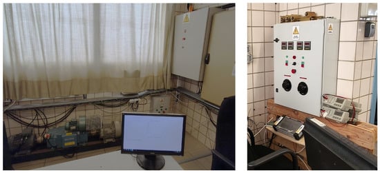
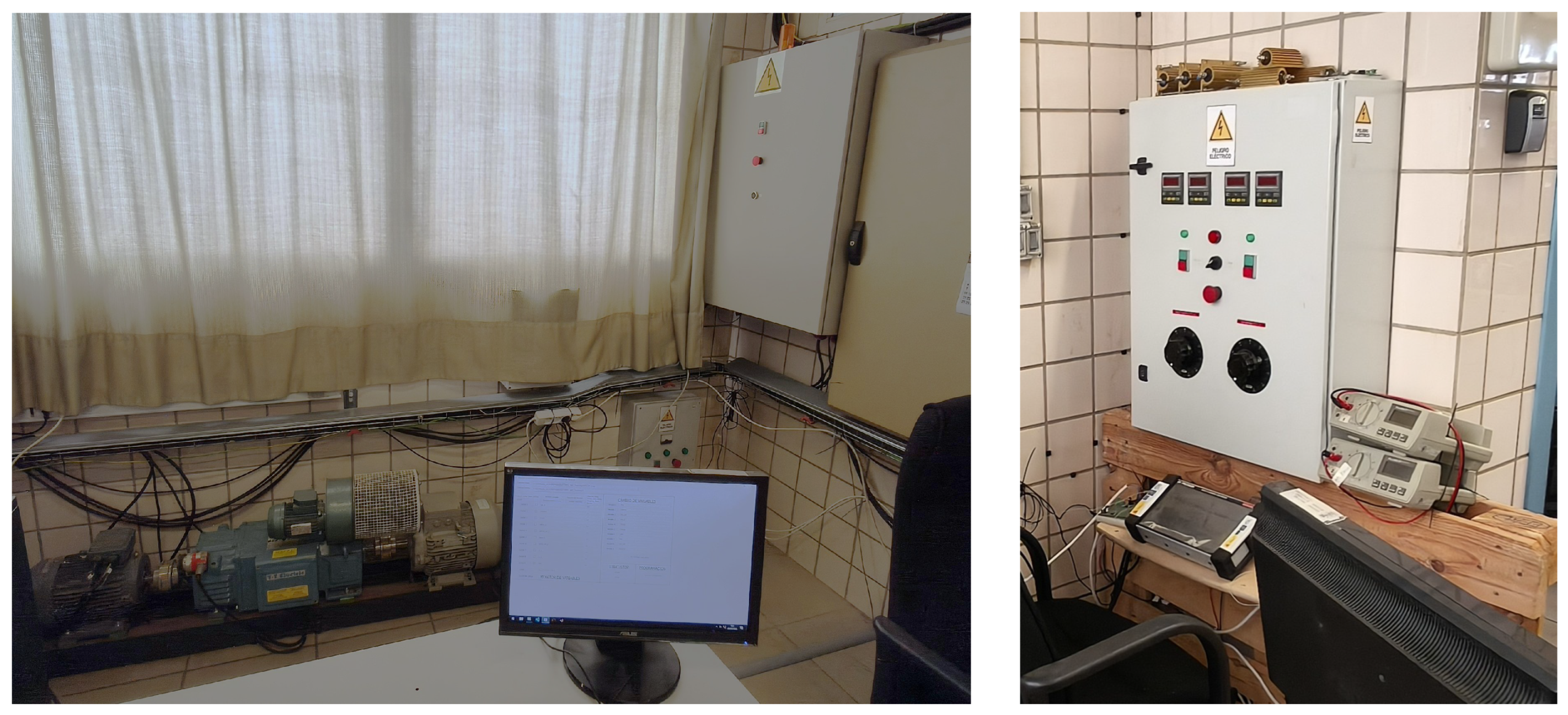
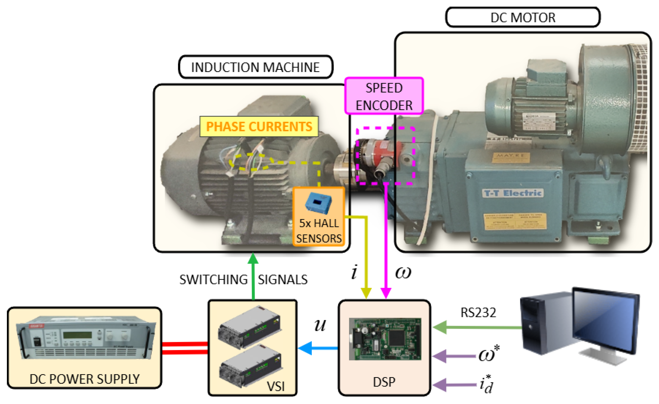
To experimentally evaluate the proposed method, a laboratory setup based on a five-phase IM is employed, as shown in Figure 2. A dedicated VSI leg supplies each of the motor phases. The inverter is composed of two standard three-phase power modules (SKS 22F, SEMIKRON GmbH, Nuremberg, Germany), with only five of their legs being used. A programmable 300-V DC power supply (Argantix Inc., San Diego, CA, USA) feeds the VSI. The control algorithm is executed in real time on a TMS320F28335 Digital Signal Processor (Texas Instruments Inc., Dallas, TX, USA), and the stator phase currents are acquired by the DSP by means of LH25-NP Hall-effect current transducers (LEM International SA, Meyrin, Switzerland).

Figure 2. Photograph of the experimental test bench: (left) induction machine (IM), DC motor, and control cabinet; (right) DC motor controller and data logger.

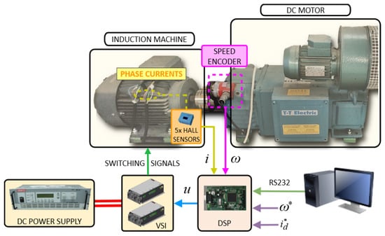
In addition, a coaxially coupled DC motor applies an opposing torque to the IM, emulating a mechanical load. Figure 3 presents a diagram of the interconnections between the different components. The main parameters of the laboratory setup are given in Table 1.

Figure 3. Diagram of the experimental test rig.

Table 1. Parameters of the induction motor.

Parameter	Value	Units
Rated power, $P_r$	1.4	kW
Rated speed, ${\omega }_r$	990	rpm
Rated current, $I_r$	2.5	A
Stator resistance, $R_s$	12.85	$\mathsf{\Omega }$
Rotor resistance, $R_r$	4.80	$\mathsf{\Omega }$
Stator leakage inductance, $L_{ls}$	79.93	mH
Rotor leakage inductance, $L_{lr}$	79.93	mH
Mutual inductance, $L_M$	681.7	mH
Number of pairs of poles, P	3	—

Effect of Predictive Control on Mechanical Variables

So far, the electrical variables have been discussed. In an aircraft, the torque, effective propulsion, and overall energy efficiency are important factors. Of those, just torque and electric efficiency depend on stator current control. The link with electrical variables is shown in the following.

The electromagnetic torque produced by the IM ($T_e$) has to counteract the opposing torque $T_L$ caused by the aerodynamic load, as well as the friction and inertia torques. Hence, $T_e=T_L+B_m{\omega }_m+J_m{\dot{\omega }}_m$, where $B_m$ and $J_m$ denote the friction and inertia values, respectively. The torque is regulated through the $d-q$ components of the stator currents. The flux component $i_{sd}^{*}$ is fixed according to the nominal flux of the machine (${\varphi }_n$), such that $i_{sd}^{*}={\varphi }_n/L_m$, whereas the quadrature component $i_{sq}^{*}$ is dynamically adjusted by the PI controller of the outer loop. Consequently, the following expressions hold in steady state:

$$T_e=T_L+B_m{\omega }_m=P{\displaystyle \frac{5}{2}}{\displaystyle \frac{L_m^2}{L_r}}{i}_{sd}^{*}{i}_{sq}^{*}$$

(18)

This allows computing the quadrature component for a certain speed as

$$i_{sq}^{*}={\displaystyle \frac{T_L+B_m{\omega }_m}{i_{sd}^{*}}}{\displaystyle \frac{L_r}{P{L}_m^2}}{\displaystyle \frac{2}{5}}$$

(19)

The relationship between mechanical speed and electrical frequency is established through the slip frequency as ${\omega }_e={\omega }_r+{\omega }_{sl}$, where field orientation is assumed and ${\omega }_{sl}={\displaystyle \frac{R_r}{L_r}}{\displaystyle \frac{i_{sq}^{*}}{i_{sd}^{*}}}$. Accordingly, the electrical speed can be expressed as

$${\omega }_e=P{\omega }_m+{\displaystyle \frac{T_L+B_m{\omega }_m}{{\left(i_{sd}^{*}\right)}^2}}{\displaystyle \frac{R_r}{P{L}_m^2}}{\displaystyle \frac{2}{5}}$$

(20)

Now, regarding the $T_L$ term, in propulsion, the torque required to turn a propeller increases roughly with the square of its rotational speed. This is due to the aerodynamic load: as the propeller’s blade spins faster, air resistance increases. The IM must supply a larger $T_e$ to counter for this increase. This is not unlike other applications of electric motors such as pumps. The outer loop of the control diagram takes care of this automatically, thus increasing the required $i_{sq}^{*}$ that is received by the inner loop.

In contrast, switching losses are governed by the switching frequency together with the magnitude of the voltage and current transitions that occur during commutation, and are usually computed as $P_{sw}=f_{sw}(E_{on}+E_{off})$ [43], with $f_{sw}$ being the switching frequency and $E_{on}$, $E_{off}$ the energies dissipated at turn-on and turn-off.

In the present case, the 5-phase IM is co-axially attached to a DC motor that acts as a load. In this way, $T_L$ is provided by the DC motor independently of speed, enabling the recreation of any flying condition in a workbench. The experiments allow assessment of the different WF selections and also the S2 (no WF) approach. In addition to tests in the real motor, some simulations will be presented. These use a standard space-state representation. A value of 80 μs is chosen for the controller as it constitutes a commonly found value in the literature [42]. The reference values for the Predictive Current Control (PCC) are sinusoidal values of frequency $f_e$ (Hz) and amplitude $I^{*}$ (A). Please note that, thanks to the experimental setup, it is possible to decouple the $f_e$ (Hz) and $I^{*}$ variables. This allows the exploration of the whole operating space of the drive.

The experimental tests were conducted by implementing the FCS-MPC algorithm in the DSP. The controller was programmed and configured from a personal computer, where the operating conditions and controller parameters for each test were established. Once the test was launched, the control algorithm was executed in real time by the DSP, while the variables of interest were recorded during steady-state operation. These variables included the stator currents in the $\alpha -\beta$ and $x-y$ subspaces, the applied voltage vector, the mechanical speed, and the relevant electrical variables of the experimental setup. After each test, the recorded data were transferred to and stored on the computer for offline processing. The measured data were subsequently used to calculate the electrical input and output power, power losses, system efficiency, and average switching frequency.

4. Results and Discussion

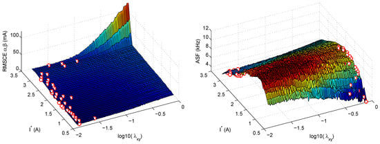
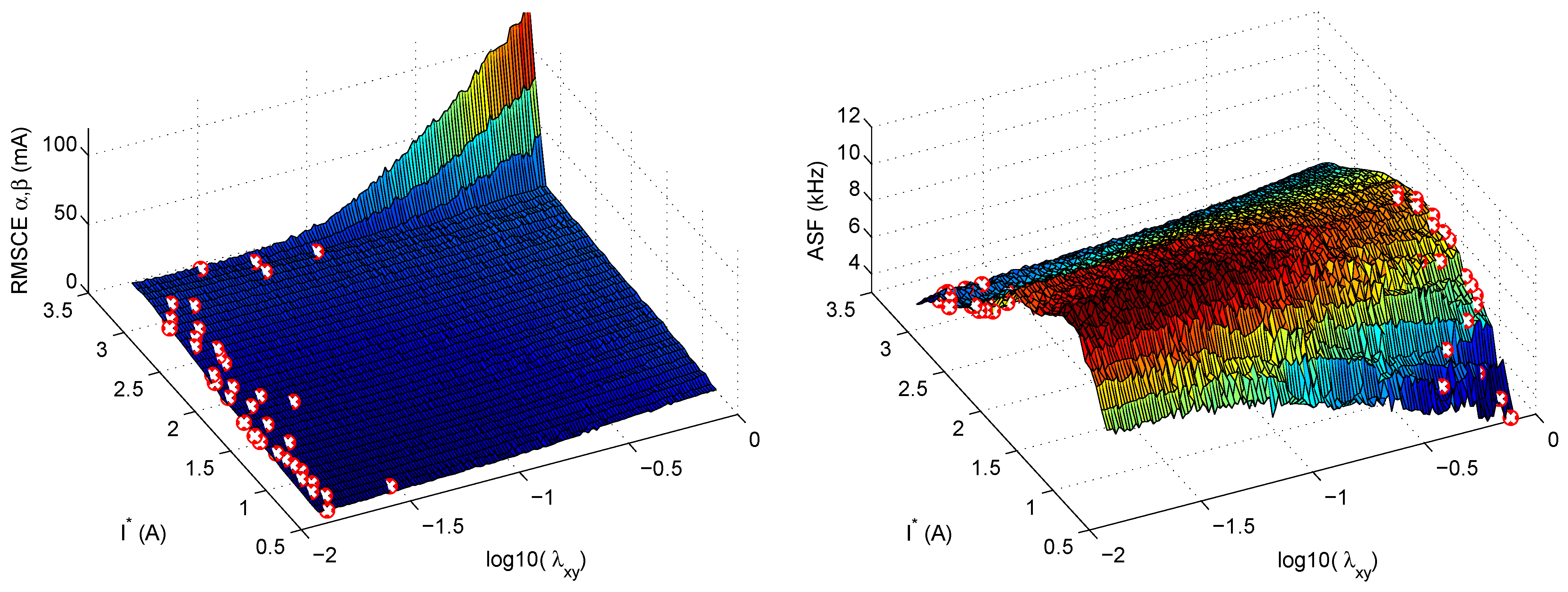
As an introductory example, an S1 class CF design method is applied first. In this case, the system behavior varies depending on the value of ${\lambda }_{xy}$. This is illustrated in Figure 4 (left), which shows the RMS control error in the $\alpha -\beta$ plane as a function of the IM load and the weighting factor ${\lambda }_{xy}$ for $f_e=60$ (Hz). Note that $f_e$ is held constant here only to simplify the presentation of the results; other values are considered in the subsequent tests. The cross (×) marks on the surface indicate the values of ${\lambda }_{xy}$ that yield the minimum error for each value of $I^{*}$. It can be observed that achieving the lowest error for different $I^{*}$ requires different values of ${\lambda }_{xy}$. Moreover, a comparison with the results in Figure 4 (right) reveals that the optimal value of ${\lambda }_{xy}$ depends on the chosen criterion: minimizing the RMSCE may result in a higher ASF, and vice versa.

Figure 4. RMSCE (left) and ASF (right) versus $I^{*}$ and the weighting factor ${\lambda }_{xy}$ (plotted on a logarithmic scale).

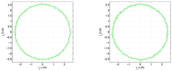
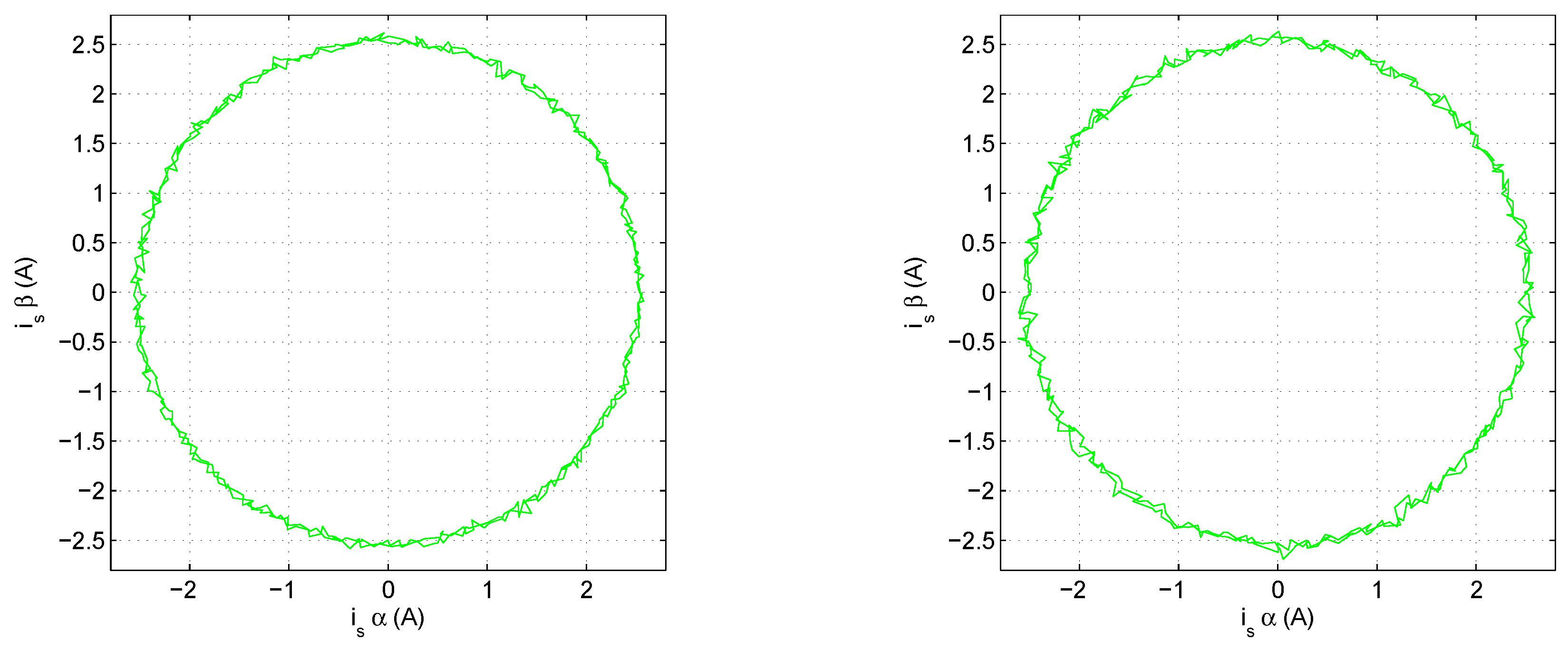
To further illustrate this case, Figure 5 presents two hodograms of $i_s$ in the $\alpha -\beta$ plane for $I^{*}=2.55$ (A) and $f_e=60$ (Hz). The left hodogram corresponds to a WF tuned to the RMSCE-optimal value for this operating point (${\lambda }_{xy}=7.1\times {10}^{-4}$), while the right one uses ${\lambda }_{xy}=0.5$, which is optimal for other operating points. This clearly shows that a fixed value of ${\lambda }_{xy}$ is not optimal for all operating points. Table 2 summarizes the system efficiency achieved for different values of ${\lambda }_{xy}$ and operating speeds. The efficiency is defined as the ratio, expressed as a percentage, between the electrical output power of the DC machine mechanically coupled to the shaft of the multiphase machine under study and the electrical input power delivered to the multiphase machine.

Figure 5. Hodograms for $i_s$ in $\alpha -\beta$ plane for two different values of ${\lambda }_{xy}$.

Table 2. System efficiency and ASF at different ${\lambda }_{xy}$ values and operating speeds.

${\mathsf{\lambda }}_{\mathit{xy}}$	@ 100 rpm	ASF [kHz]	@ 200 rpm	ASF [kHz]	@ 500 rpm	ASF [kHz]	@ 750 rpm	ASF [kHz]
0.01	4.26	3.38	7.97	3.37	19.33	3.09	28.61	2.26
0.2	6.20	3.65	9.99	3.66	23.57	3.32	30.47	2.35
0.5	5.76	4.16	11.02	4.16	24.21	3.89	30.99	2.82
1	5.23	4.37	10.54	4.52	24.20	4.34	31.32	3.41
5	4.62	5.53	9.75	5.17	22.02	5.22	27.93	4.38

The above results can be compared with the CF using the S2 design category. In this case, no WF tuning is required. Using $f_e=60$ Hz, as in the previous cases, the results shown in Figure 6 are obtained. When compared with Figure 4, it can be seen that under certain operating conditions the S2 strategy achieves better ASF results at the cost of a higher RMSCE, while under other conditions the reverse behavior occurs. To facilitate the comparison with S1 Figure 6 also portraits results with an S1 CF with ${\lambda }_{xy}=0.2$ and ${\lambda }_{xy}=2.2$. It can be seen that one of the S1 cases performs better than S2 w.r.t. RMSCE but worse for ASF, whereas the other S1 case performs worse than S2 w.r.t. RMSCE but better for ASF. Hence, the S2 results represent a trade-off between S1 with ${\lambda }_{xy}=0.2$ and S1 with ${\lambda }_{xy}=2.2$. Consequently, the performance of the S2 strategy is comparable to that of S1, but it does not surpass it.

Figure 6. RMSCE (left) and ASF (right) versus $I^{*}$ for S2 (solid red lines), S1 with ${\lambda }_{xy}=0.02$ (dotted black lines), and S1 with ${\lambda }_{xy}=2.2$ (dashed blue lines).

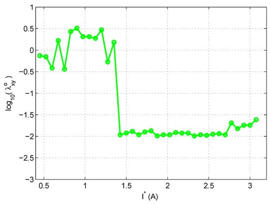
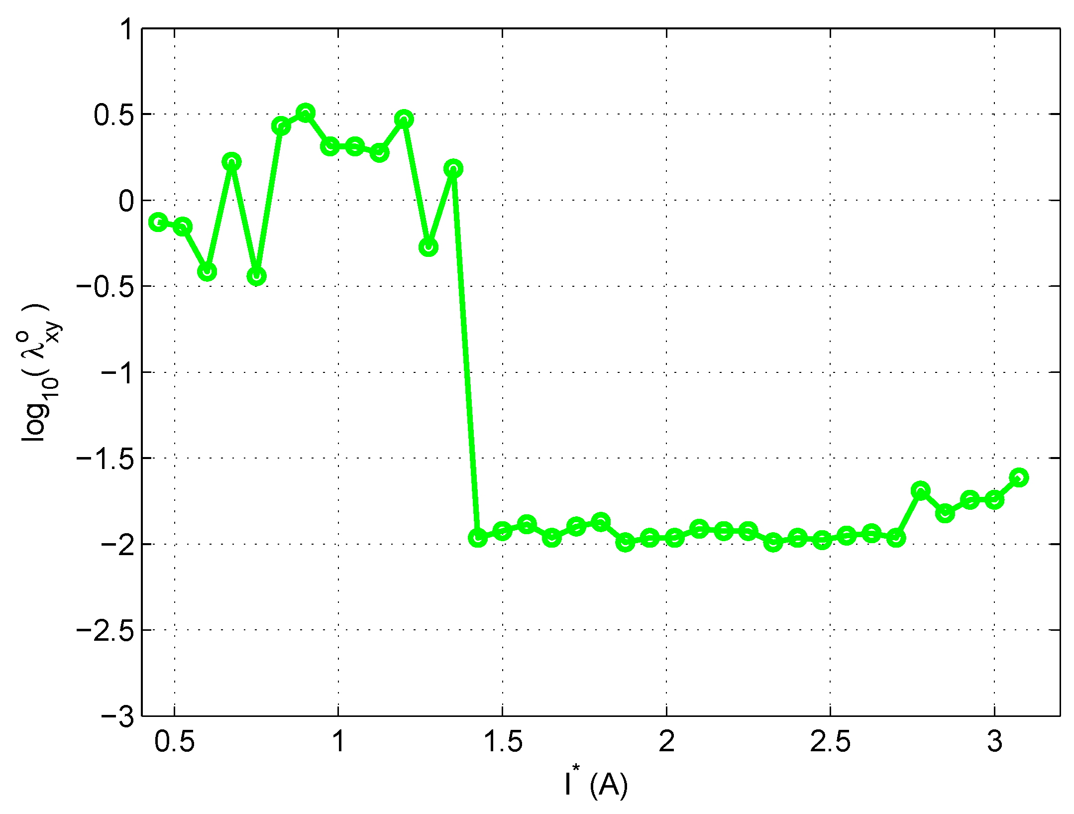
Finally, the S3 CF design method is assessed. Note that this method requires the ${\gamma }_i$ coefficients to be defined. For the sake of a simpler comparison, ${\gamma }_2=0$ is chosen, so that only RMSCE and ASF are taken into account as figures of merit. As these two quantities span different ranges, each of them is normalized by its maximum value. Accordingly, the meta-CF used in the simulations is

$${\lambda }_{xy,i}^o=\underset{{\lambda }_{xy}}{\mathrm{argmin}}RMSC{E}_n+{\gamma }_1·AS{F}_n$$

(21)

where $RMSC{E}_n=RMSCE/\left(\max RMSCE\right)$ and $AS{F}_n=ASF/\left(\max ASF\right)$. For simplicity, only a single frequency, $f_e=60$ Hz, is considered (note that the analysis can be readily extended to other frequencies). Figure 7 shows the ${\lambda }_{xy,i}^o$ values as a function of $I_i^{*}$, which will be used in the subsequent simulations.

Figure 7. Optimal values of ${\lambda }_{xy}$ for each $I^{*}$ and $f_e=60$ (Hz).

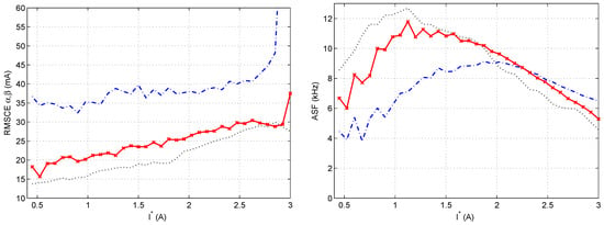
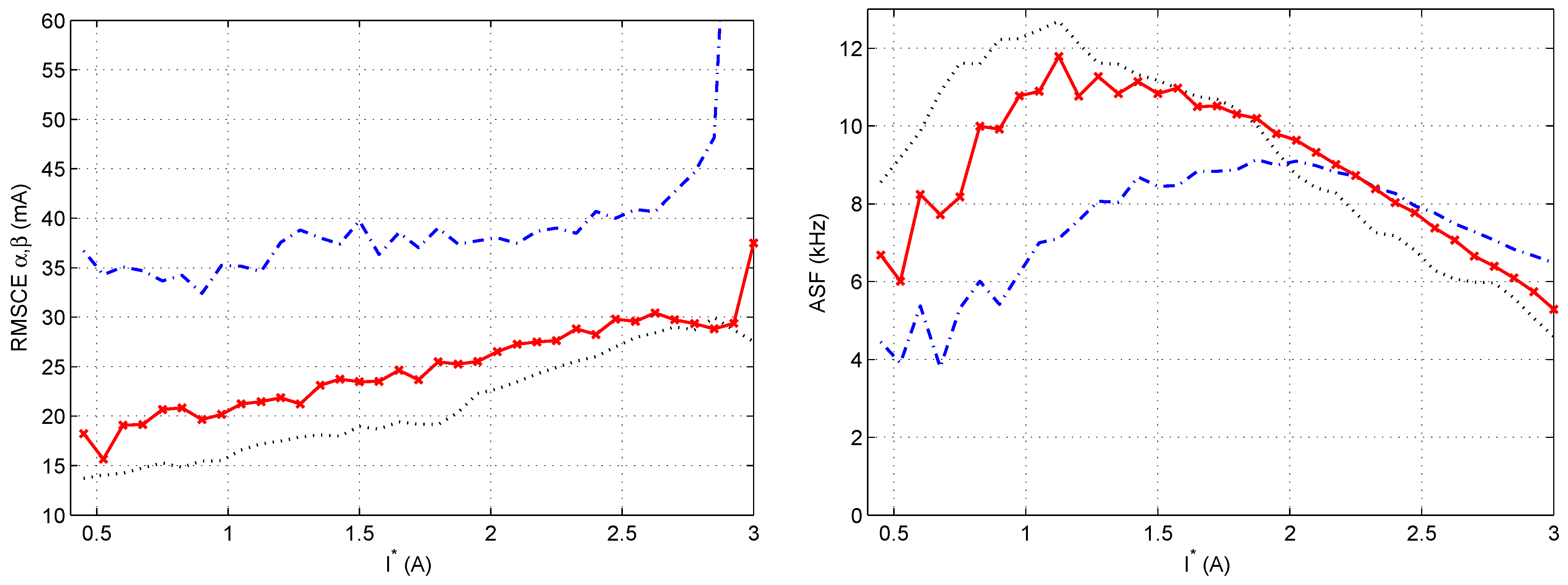
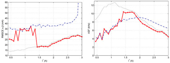
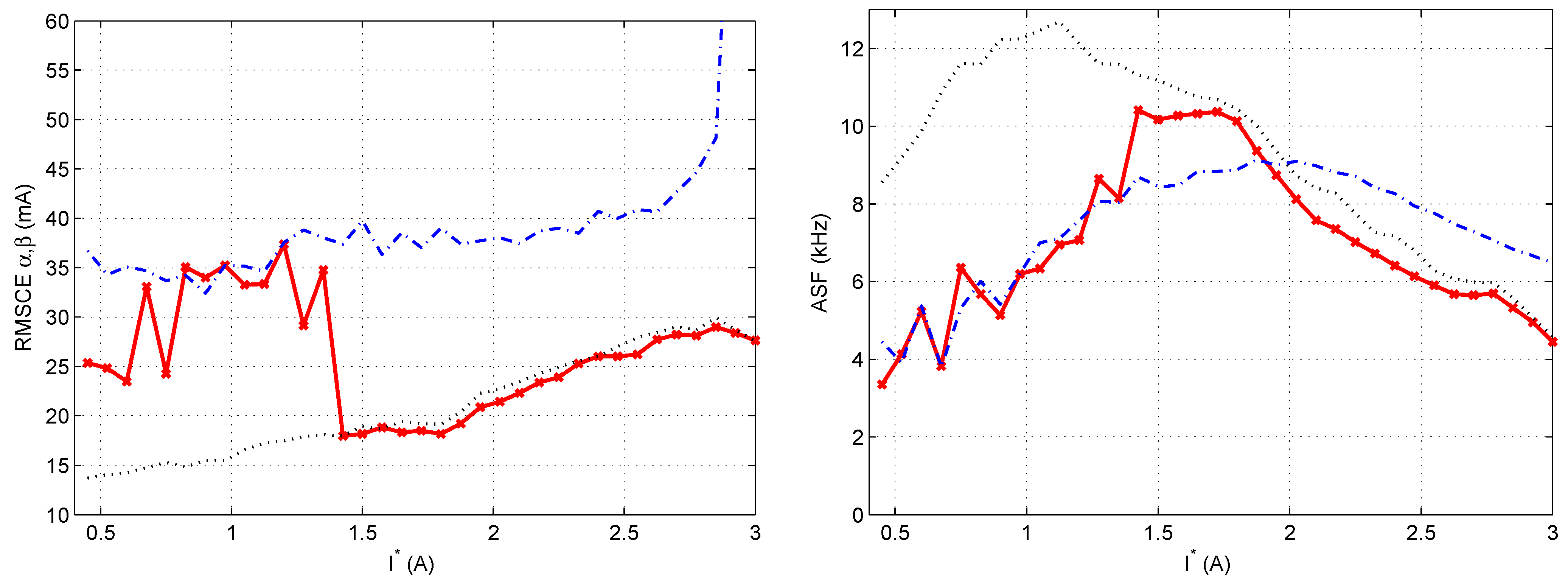
Figure 8 presents the results achieved by the PCC with the S3 strategy and ${\gamma }_1=0.4$. As in the previous case, two S1-based results are included as a reference, using the same ${\lambda }_{xy}$ values as before. A comparison with Figure 6 clearly shows that, across most of the operating range, S3 performs better than both S1 and S2, providing a lower or similar error together with a lower or similar switching frequency.

Figure 8. RMSCE (left) and ASF (right) versus $I^{*}$ for S3 (solid red line), S1 with ${\lambda }_{xy}=0.02$ (dotted black lines), and S1 with ${\lambda }_{xy}=2.18$ (dashed blue lines).

Table 3 quantifies, for $f_e=50$ Hz, the tracking accuracy illustrated for $f_e=60$ Hz in the left-hand plots of Figure 6 and Figure 8. It indicates that S2 worsens the RMSCE with respect to S1 with ${\lambda }_{xy}=0.2$ at every operating point, but improves it with respect to ${\lambda }_{xy}=2.2$. S3 improves the RMSCE with respect to S1 across most of the operating range, with the exception of the region around $I^{*}\approx 0.6$–$0.9$ A. On the other hand, Table 4 quantifies, also for $f_e=50$ Hz, the ASF shown in the right-hand plots of the same figures. It indicates that S2 improves the ASF with respect to ${\lambda }_{xy}=0.2$ in almost all cases, but worsens it with respect to ${\lambda }_{xy}=2.2$ in most of them. S3 also improves the ASF with respect to ${\lambda }_{xy}=0.2$ in almost all cases, whereas with respect to ${\lambda }_{xy}=2.2$ it does so only at some of the operating points.

Table 3. RMSCE [mA] in $\alpha \beta$ subspace at representative operating points, for $f_e=50$ Hz. ${\mathsf{\Delta }}_{0.2}$ and ${\mathsf{\Delta }}_{2.2}$ denote the percentage change with respect to S1 with ${\lambda }_{xy}=0.2$ and ${\lambda }_{xy}=2.2$, respectively; positive values indicate a reduction of the error.

${\mathit{I}}^{*}$ (A)	S1		S2			S3
	${\mathsf{\lambda }}_{\mathit{xy}}=\mathbf{0.2}$	${\mathsf{\lambda }}_{\mathit{xy}}=\mathbf{2.2}$	RMSCE	${\mathsf{\Delta }}_{\mathbf{0.2}}$ (%)	${\mathsf{\Delta }}_{\mathbf{2.2}}$ (%)	RMSCE	${\mathsf{\Delta }}_{\mathbf{0.2}}$ (%)	${\mathsf{\Delta }}_{\mathbf{2.2}}$ (%)
0.5	19.5	34.2	25.0	$-28.4$	$+27.0$	19.5	$0.0$	$+43.2$
1.0	21.1	35.5	28.3	$-33.9$	$+20.3$	18.5	$+12.7$	$+48.0$
1.5	20.2	36.5	28.4	$-40.2$	$+22.2$	11.4	$+43.8$	$+68.8$
2.0	23.6	36.4	30.5	$-29.5$	$+16.2$	15.5	$+34.3$	$+57.5$
2.5	24.7	38.1	33.5	$-35.4$	$+12.0$	18.7	$+24.2$	$+50.8$
3.0	27.1	37.7	35.9	$-32.5$	$+4.8$	22.4	$+17.3$	$+40.6$

Table 4. ASF [kHz] at the same operating points, for $f_e=50$ Hz. ${\mathsf{\Delta }}_{0.2}$ and ${\mathsf{\Delta }}_{2.2}$ denote the percentage change with respect to S1 with ${\lambda }_{xy}=0.2$ and ${\lambda }_{xy}=2.2$, respectively; positive values indicate a reduction of the switching effort.

${\mathit{I}}^{*}$ (A)	S1		S2			S3
	${\mathsf{\lambda }}_{\mathit{xy}}=\mathbf{0.2}$	${\mathsf{\lambda }}_{\mathit{xy}}=\mathbf{2.2}$	ASF	${\mathsf{\Delta }}_{\mathbf{0.2}}$ [%]	${\mathsf{\Delta }}_{\mathbf{2.2}}$ [%]	ASF	${\mathsf{\Delta }}_{\mathbf{0.2}}$ [%]	${\mathsf{\Delta }}_{\mathbf{2.2}}$ [%]
0.5	6.06	4.17	3.60	$+40.6$	$+13.6$	6.06	$+0.0$	$-45.4$
1.0	10.61	7.09	8.04	$+24.2$	$-13.4$	10.18	$+4.0$	$-43.6$
1.5	13.01	9.74	10.60	$+18.5$	$-8.7$	7.33	$+43.7$	$+24.8$
2.0	12.54	10.77	11.75	$+6.2$	$-9.1$	11.82	$+5.7$	$-9.7$
2.5	11.03	10.52	10.76	$+2.5$	$-2.3$	7.06	$+36.0$	$+32.8$
3.0	8.74	9.27	9.16	$-4.8$	$+1.2$	6.64	$+24.1$	$+28.5$

Taken together, the two tables show that the two metrics are linked by the choice of ${\lambda }_{xy}$ in S1, and that S2 inherits this link even though it uses no weighting factor: at each operating point an improvement in one metric is offset by a degradation in the other, so S2 selects a different compromise between the two objectives, not a better one. In contrast, S3 improves both metrics simultaneously with respect to S1 with ${\lambda }_{xy}=0.2$ for almost tested operating points and with respect to the ${\lambda }_{xy}=2.2$ case for more of them.

The results confirm that the optimal value of the WF ${\lambda }_{xy}$ is not unique, as it depends both on the operating point (Figure 4) and on the criterion used to define optimality. In particular, the values that minimize RMSCE differ from those that minimize ASF. This result agrees with the trade-offs among figures of merit reported in earlier studies on FSMPC of multiphase drives [37,38]. Consequently, the common practice of selecting a single constant value (e.g., ${\lambda }_{xy}=0.5$) necessarily leads to suboptimal performance over part of the operating range, as illustrated by the hodograms in Figure 5.

The ranking-based scheme (S2) eliminates the need for an explicit weighting factor, which is advantageous in terms of design effort. However, the experimental comparison shows that its performance lies between that of the S1 configurations with low and high ${\lambda }_{xy}$ values, effectively behaving as a fixed compromise solution. The WF has not really disappeared; it has been implicitly embedded in the sorting and ranking operations. This means that the designer loses the ability to steer the closed-loop behavior towards a particular objective, such as energy efficiency, which is of primary interest in electric aircraft propulsion. In addition, since similar trade-off characterizations do not exist for WF-free methods, the practitioner cannot easily predict where in the trade-off curve the S2 solution will land.

The operating-point-dependent selection (S3) outperforms both S1 and S2 for most of the operating range, producing lower or similar tracking error with lower or similar switching frequency. The price to pay is an off-line characterization phase, in which the meta cost function (21) is minimized for a grid of operating points, and the need to select the meta weighting factor ${\gamma }_1$. It should be noted that this selection is performed at a higher level and only once, using figures of merit (RMSCE, ASF) that have a direct physical interpretation and a direct link to drive efficiency [19], which makes the choice easier than the direct selection of ${\lambda }_{xy}$.

It should be noted that incorporating a figure of merit such as ASF into the FSMPC cost function J, as some works do, does not guarantee that this figure of merit is properly taken into account. On the contrary, because the controller has access to only a limited number of configurations and conflicting criteria may be included in J, the resulting control action may be optimal according to (8) while still being suboptimal in terms of the overall drive performance. Therefore, the WF tuning in (16) remains necessary even in such cases.

Extension to Other Operating Points

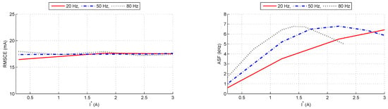
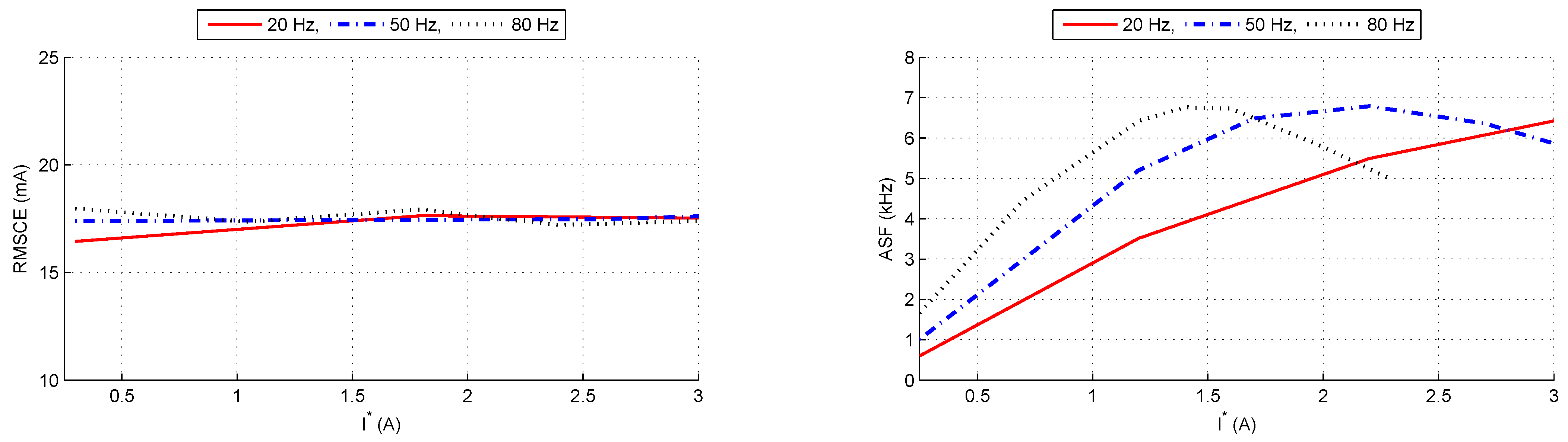
So far, the cases of $f_e=50$ Hz and $f_e=60$ Hz have been presented. The analysis can, of course, be performed for other electrical frequencies, and the corresponding results are presented next. As a first step, it is interesting to look at the RMSCE and ASF maps for different combinations of $I^{*}$ and $f_e$. These maps are shown in Figure 9 where a constant WF (${\lambda }_{xy}=0.7$) is used. It can be seen that the controller keeps the RMSCE around certain values; however, the ASF experiences significant changes depending on both the frequency and the amplitude of stator currents. This supports the idea that adapting the WF can provide advantages.

Figure 9. Curves of RMSCE (left) and ASF (right) using S1 with ${\lambda }_{xy}=0.7$. Each curve correspond to a $f_e$ value as indicated by the legend at the top.

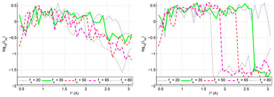
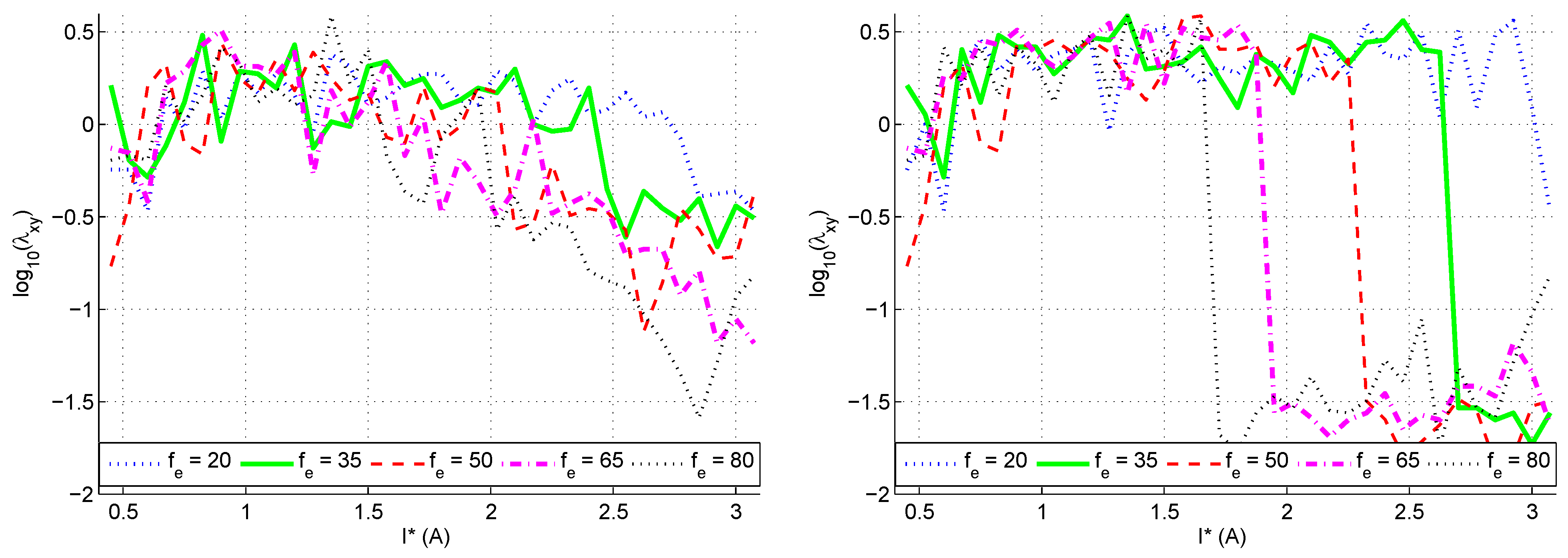
Now, following the same procedure as in the constant $f_e$ case, the optimal WF is calculated. The results are presented in Figure 10. Notice that a logarithmic scale is used for the WF as this factor can take values spanning from ${10}^{-2}$ to ${10}^{0.5}$. It is worth highlighting the flexibility that the choice of ${\gamma }_1$ gives to the proposed approach. In particular, in said Figure 10, the left graph corresponds to ${\gamma }_1=1$, corresponding to a significant penalization for the switching frequency. This is adequate in cases where the ASF needs to be low (for hardware requirements or to lessen the commutation losses). In other situations, one can increase ${\gamma }_1$ with the results shown in the right part of Figure 10 where lower values of the WF are allowed resulting in less RMSCE and higher ASF.

Figure 10. Optimal values of the WF for varying I and for several frequencies $f_e$. The left graph corresponds to ${\gamma }_1=1$. The right graph is for ${\gamma }_1=0.25$.

5. Conclusions

Three CF design strategies for the stator current controller based on FSMPC in a five-phase induction machine have been experimentally compared: a conventional constant WF (S1), a ranking-based WF free scheme (S2), and an operating-point-dependent WF selection based on the off line minimization of a meta CF that combines tracking error and switching frequency (S3).

The results demonstrate that no constant WF provides optimal performance over the entire tested operating range, since the value of ${\lambda }_{xy}$ that minimizes RMSCE differs both from the one that minimizes ASF and across operating points. The ranking-based scheme does not resolve this tension. Although S2 removes the explicit WF, the trade-off survives inside the sorting and ranking operations: at every tested operating point, its improvement in one metric is offset by a degradation in the other, and its performance lies between the two S1 configurations used as reference (${\lambda }_{xy}=0.2$ and ${\lambda }_{xy}=2.2$). S2 therefore constitutes a different compromise, not a better one. It should be noted that this comparison uses two representative constant WFs rather than the point-wise optimal ${\lambda }_{xy}$ of Figure 7; establishing whether S2 can match the best achievable S1 performance, and not merely interpolate between two fixed settings, would require that stronger baseline.

The proposed S3 strategy breaks this constraint. Averaged over the tested operating points of Table 3 and Table 4, it reduces the RMS control error by $22\%$ and $51\%$ with respect to the ${\lambda }_{xy}=0.2$ and ${\lambda }_{xy}=2.2$ configurations, while reducing the ASF by $19\%$ with respect to the former and leaving it essentially unchanged with respect to the latter. More significantly than the averages, S3 improves both metrics simultaneously with respect to ${\lambda }_{xy}=0.2$ at every tested operating point above $I^{*}=1.2$ A, a combination that no single constant WF can deliver, since in S1 any reduction of one metric is paid for in the other.

Two limitations delimit this result, both traceable to the design of the meta CF rather than to the scheduling principle itself. Below $I^{*}\approx 0.6$ A, the scheduled WF converges to ${\lambda }_{xy}\approx 0.2$, so S3 degenerates into the corresponding S1 configuration and offers no advantage in that region. Around $I^{*}\approx 0.75$–$0.9$ A, the minimization of the meta CF favors switching reduction at the expense of tracking accuracy, which follows from the particular value of ${\gamma }_1$ adopted here; a different ${\gamma }_1$, or one scheduled with the operating point, would displace this region at the cost of an additional parameter to characterize. Since ${\gamma }_1$ was taken from previous work [19] rather than re-derived for this setup, the reported gains are conditional on that choice, although selecting it is arguably easier than selecting ${\lambda }_{xy}$ directly because RMSCE and ASF carry direct physical meaning. A third, practical limitation is that the offline characterization effort grows with the number of operating variables considered.

Finally, the efficiency-related claims of this work are based on ASF as an indicator of switching losses, together with the system efficiency of Table 2; the drive losses themselves were not measured as a function of ${\lambda }_{xy}$ across the operating range. The conclusion that S3 favors drive efficiency is therefore an inference from the simultaneous reduction of tracking error and switching frequency rather than a directly verified efficiency result. Future work will address the extension of the scheduling to additional operating variables, such as speed or torque, and to cost functions with further terms, together with direct loss measurements that would quantify the efficiency improvement these results suggest.

References

- Rault, J.; Richalet, A.; Testud, J.; Papon, J. Model predictive heuristic control: Applications to industrial processes. Automatica 1978, 14, 413–428. [Google Scholar]
- Rodríguez, J.; Cortés, P. Predictive Control of Power Converters and Electrical Drives. In Predictive Control of Power Converters and Electrical Drives; John Wiley & Sons, Ltd.: Hoboken, NJ, USA, 2012; Chapter 3. [Google Scholar]
- Holtz, J. A predictive controller for the stator current vector of AC machines fed from a switched voltage source. In Proceedings of the First International Power Electronics Conference in Asia (IPEC-Tokyo 1983), Tokyo, Japan, 27 March–1 April 1983; pp. 1665–1675. [Google Scholar]
- Lim, C.S.; Levi, E.; Jones, M.; Rahim, N.A.; Hew, W.P. A comparative study of synchronous current control schemes based on FCS-MPC and PI-PWM for a two-motor three-phase drive. IEEE Trans. Ind. Electron. 2013, 61, 3867–3878. [Google Scholar] [CrossRef] [Scilit]
- Arahal, M.R.; Barrero, F.; Ortega, M.G.; Martin, C. Harmonic analysis of direct digital control of voltage inverters. Math. Comput. Simul. 2016, 130, 155–166. [Google Scholar] [CrossRef] [Scilit]
- Scaglione, G.; Nevoloso, C.; Schettino, G.; Di Tommaso, A.O.; Miceli, R.; Knoblach, J.; Dietz, A. A Novel Voltage Vectors Subset-Based Model Predictive Control for Six-Phase PMSM drives. In Proceedings of the 2024 International Conference on Electrical Machines (ICEM), Torino, Italy, 1–4 September 2024; pp. 1–7. [Google Scholar]
- Tenconi, A.; Rubino, S.; Bojoi, R. Model predictive control for multiphase motor drives–a technology status review. In Proceedings of the 2018 International Power Electronics Conference (IPEC-Niigata 2018-ECCE Asia); IEEE: New York City, NY, USA, 2018; pp. 732–739. [Google Scholar]
- Zhou, H.; Xiang, X.; Li, Y.; Tao, T. Simplified Model Predictive Current Control for Dual Three-Phase PMSM with Low Computation Burden and Switching Frequency. CES Trans. Electr. Mach. Syst. 2024, 8, 447–454. [Google Scholar] [CrossRef] [Scilit]
- Gębura, A.; Szelmanowski, A.; Jacyna-Gołda, I.; Gołda, P.; Kalbarczyk, M.; Tomaszewska, J. Concepts and experiments on more electric aircraft power systems. Energies 2025, 18, 1653. [Google Scholar] [CrossRef] [Scilit]
- Frikha, M.A.; Croonen, J.; Deepak, K.; Benômar, Y.; El Baghdadi, M.; Hegazy, O. Multiphase Motors and Drive Systems for Electric Vehicle Powertrains: State of the Art Analysis and Future Trends. Energies 2023, 16, 768. [Google Scholar] [CrossRef] [Scilit]
- Yu, F.; Chen, J.; Gao, P.; Kong, Y.; Sun, X.; Wang, J.; Chen, X. A Review of Hybrid-Electric Propulsion in Aviation: Modeling Methods, Energy Management Strategies, and Future Prospects. Aerospace 2025, 12, 895. [Google Scholar] [CrossRef] [Scilit]
- Shaik, J.; Chudamani, R. Empirical Open-Phase Fault Model for PC-FPIM and Comparative Fault Tolerance Evaluation Against Star Configuration. Int. J. Circuit Theory Appl. 2026, 1–13. [Google Scholar] [CrossRef] [Scilit]
- Arahal, M.R.; Barrero, F.; Bermúdez, M.; Satué, M.G. Predictive Stator Current Control of a Five-phase Motor using a Hybrid Control Set. IEEE J. Emerg. Sel. Top. Power Electron. 2022, 11, 1444–1453. [Google Scholar] [CrossRef] [Scilit]
- Bessaad, T.; Latrouche, M.; Bothtache, A.A.; Khati, A.; Benaicha-Mati, K. A Comparative Study of Controller Performance in Five-Phase Induction Motor Drives. Eurasia Proc. Sci. Technol. Eng. Math. 2026, 39, 9–18. [Google Scholar] [CrossRef] [Scilit]
- Laksar, J.; Komrska, T.; Suchỳ, O.; Šmídl, V. Voltage Zero-Sequence Components in Optimal Control of Five-Phase PMSM Drives. In Proceedings of the IECON 2025—51st Annual Conference of the IEEE Industrial Electronics Society; IEEE: New York City, NY, USA, 2025; pp. 1–6. [Google Scholar]
- Levi, E. Multiphase electric machines for variable-speed applications. IEEE Trans. Ind. Electron. 2008, 55, 1893–1909. [Google Scholar] [CrossRef] [Scilit]
- Ouanouki, A.; Kouzi, K.; Difi, D.; Ghibeche, M. Predictive Control Strategy for Two Five-Phase Permanent Magnet Synchronous Motors Connected in Series Powered by A Single Inverter. Int. J. Robot. Control Syst. 2025, 5, 2311–2324. [Google Scholar] [CrossRef] [Scilit]
- Carrillo-Rios, J.; Cordoba-Ramos, M.; Lara-Lopez, R.; Gonzalez-Prieto, I.; Duran, M.J.; Aciego, J.J.; Mora-Moreno, P.; Gonzalez-Prieto, A. Multivector model predictive control for multiphase induction machines with dead-time knowledge. Sci. Rep. 2026, 16, 11686. [Google Scholar] [CrossRef] [Scilit] [PubMed]
- Marsal, E.; Arahal, M.R.; Satué, M.G.; Rouzbehi, K. Effect of Weighting Factors in Energy Efficiency of Predictive Control of Multi-Phase Drives. Appl. Sci. 2025, 15, 12148. [Google Scholar] [CrossRef] [Scilit]
- Atanasov, G.; Silberhorn, D. Bridging scale and sustainability: A battery-electric aircraft with range extenders for flexible short-to medium-range operations. Eng. Proc. 2026, 133, 70. [Google Scholar] [CrossRef] [Scilit]
- Jayan, V.; Ghias, A.M. Weighting Factor Free Model Predictive Control for a Flying Capacitor Converter in a DC Microgrid. IEEE Trans. Energy Convers. 2021, 37, 1030–1041. [Google Scholar] [CrossRef] [Scilit]
- Serra, J.; Cardoso, A.J.M. A simplified model predictive control for asymmetrical six-phase induction motors that eliminates the weighting factor. Machines 2022, 10, 1189. [Google Scholar] [CrossRef] [Scilit]
- Eshwar, K.; Thippiripati, V.K. Weighting-factorless predictive torque control scheme for dual inverter fed open-end-winding PMSM with single DC source. IEEE Trans. Power Electron. 2021, 36, 12968–12978. [Google Scholar] [CrossRef] [Scilit]
- Meza, G.R.; Ferragud, X.B.; Saez, J.S.; Durá, H. Controller Tuning with Evolutionary Multiobjective Optimization; Springer: Cham, Switzerland, 2017. [Google Scholar]
- Arahal, M.R.; Barrero, F.; Satué, M.G.; Bermúdez, M. Fast finite-state predictive current control of electric drives. IEEE Access 2023, 11, 12821–12828. [Google Scholar] [CrossRef] [Scilit]
- Yin, R.; Yang, J. Predictive current control for seven-phase induction motor based on the optimal operating time of four-dimensional vector. IET Electr. Power Appl. 2019, 13, 1684–1695. [Google Scholar] [CrossRef] [Scilit]
- Zhang, Y.; Jia, D.; Yin, Z.; Luo, P. GRA-TOPSIS-Based Model Predictive Torque Control for Induction Motor Without Weighting Factors. IEEE Trans. Power Electron. 2025, 40, 12309–12320. [Google Scholar] [CrossRef] [Scilit]
- Vujji, A.; Gupta, Y.B.S.S.; Dahiya, R.; Bhaskar, M.S.; Khan, B. Experimental verification for cost function optimization using TOPSIS approach for predictive control of surface mounted PMSM. IET Power Electron. 2023, 16, 948–960. [Google Scholar] [CrossRef] [Scilit]
- Li, H.; Xu, H.; Xie, H. A Model Predictive Torque Control with Power Factor Improvement without Weighting Factor Adjustment. IEEE Trans. Energy Convers. 2024, 40, 1763–1772. [Google Scholar] [CrossRef] [Scilit]
- Guazzelli, P.R.U.; de Andrade Pereira, W.C.; de Oliveira, C.M.R.; de Castro, A.G.; de Aguiar, M.L. Weighting factors optimization of predictive torque control of induction motor by multiobjective genetic algorithm. IEEE Trans. Power Electron. 2019, 34, 6628–6638. [Google Scholar] [CrossRef] [Scilit]
- Arshad, M.H.; Abido, M.A.; Salem, A.; Elsayed, A.H. Weighting factors optimization of model predictive torque control of induction motor using NSGA-II with TOPSIS decision making. IEEE Access 2019, 7, 177595–177606. [Google Scholar] [CrossRef] [Scilit]
- Davari, S.A.; Khaburi, D.A.; Kennel, R. Using a weighting factor table for FCS-MPC of induction motors with extended prediction horizon. In Proceedings of the IECON 2012-38th Annual Conference on IEEE Industrial Electronics Society; IEEE: New York City, NY, USA, 2012; pp. 2086–2091. [Google Scholar]
- Liu, X.; Qiu, L.; Wu, W.; Ma, J.; Fang, Y.; Peng, Z.; Wang, D. Neural predictor-based low switching frequency FCS-MPC for MMC with online weighting factors tuning. IEEE Trans. Power Electron. 2021, 37, 4065–4079. [Google Scholar] [CrossRef] [Scilit]
- Deng, A.; Yang, W.; Hu, G.; Huang, W.; Xu, D. Reinforcement Learning based Weight-Tuning Model Predictive Control of Permanent Magnet Synchronous Motor. In Proceedings of the 2024 IEEE 10th International Power Electronics and Motion Control Conference (IPEMC2024-ECCE Asia); IEEE: New York City, NY, USA, 2024; pp. 317–322. [Google Scholar]
- Shahid, M.B.; Jin, W.; Abbasi, M.A.; Li, L.; Rasool, A.; Bhatti, A.R.; Hussen, A.S. Optimal weighting factor design based on entropy technique in finite control set model predictive torque control for electric drive applications. Sci. Rep. 2024, 14, 12791. [Google Scholar] [CrossRef] [Scilit] [PubMed]
- Ait Ali, Y.; Ouassaid, M. Optimal FCS-MPC Cost Function Dimension Unification for Optimizing Operating Conditions of DFIG-Based Wind Turbine Power Converters. IEEE Trans. Ind. Appl. 2025, 62, 6779–6794. [Google Scholar] [CrossRef] [Scilit]
- Fretes, H.; Rodas, J.; Doval-Gandoy, J.; Gomez, V.; Gomez, N.; Novak, M.; Rodriguez, J.; Dragičević, T. Pareto Optimal Weighting Factor Design of Predictive Current Controller of a Six-Phase Induction Machine based on Particle Swarm Optimization Algorithm. IEEE J. Emerg. Sel. Top. Power Electron. 2021, 10, 207–219. [Google Scholar] [CrossRef] [Scilit]
- Arahal, M.R.; Satué, M.G.; Barrero, F.; Ortega, M.G. Adaptive cost function FCSMPC for 6-phase IMs. Energies 2021, 14, 5222. [Google Scholar] [CrossRef] [Scilit]
- Yang, X.; Li, J.; Wang, K.; Kim, U.; Zhang, Z.; Park, K.B. A weighting factor design approach for FCS-MPC techniques based on PSO and k-means algorithm. In Proceedings of the 2022 IEEE Energy Conversion Congress and Exposition (ECCE); IEEE: New York City, NY, USA, 2022; pp. 1–8. [Google Scholar]
- Yang, T.; Wang, Y.; Miao, Y.; Xu, Q.; Guo, Q. A novel weighting factor determined method of model predictive torque control for permanent magnet synchronous motor. IET Electr. Power Appl. 2024, 18, 1616–1625. [Google Scholar] [CrossRef] [Scilit]
- Kowal Gornig, A.; Arahal, M.R.; Barrero, F. Tuning of Predictive Controllers for Five-Phase Drives. Int. J. Eng. Adv. Technol. (IJEAT) 2018, 8, 57–63. [Google Scholar]
- Satué, M.G.; Arahal, M.R.; Ortega, M.G.; Ramírez, D.R. A simple rotor current estimation method for predictive control of multi-phase drives. Int. J. Circuit Theory Appl. 2022, 50, 4478–4491. [Google Scholar] [CrossRef] [Scilit]
- Azpúrua, M.A.; Pous, M.; Silva, F. Time- and Frequency-Domain Characterization of Switching Losses in GaN FETs Power Converters. IEEE Trans. Power Electron. 2022, 37, 3219–3232. [Google Scholar] [CrossRef] [Scilit]
Disclaimer/Publisher’s Note: The statements, opinions and data contained in all publications are solely those of the individual author(s) and contributor(s) and not of MDPI and/or the editor(s). MDPI and/or the editor(s) disclaim responsibility for any injury to people or property resulting from any ideas, methods, instructions or products referred to in the content. |
© 2026 by the authors. Licensee MDPI, Basel, Switzerland. This article is an open access article distributed under the terms and conditions of the Creative Commons Attribution (CC BY) license.