Screening Electric-Vehicle Charging Against Positive Model-to-Meter Renewable-Energy Residuals: Smart G2V Potential and a V2G Capacity Envelope

Abstract

This study develops a deterministic annual screening model for matching electric-vehicle (EV) charging demand with the positive part of modelled minus metered renewable-energy production. Distribution-system-operator-supplied records for photovoltaic (PV), wind and hydropower installations in 2020–2025 were combined with a supplier-provided extract from the Central Register of Vehicles and Drivers (CEPiK) covering 30 models and 20,043 vehicles. The corrected calculation assigns each technology–year–capacity-class residual once across the full fleet, then applies energy, charger-power, connection and availability limits. Annual source-side demand is 54.389 GWh. In the 2025 large-source cases, Smart G2V covers 46.31% of demand for PV, 64.36% for hydropower and 100.00% for wind, compared with 16.21%, 22.53% and 98.97% under immediate charging. Wind offers 249.660 GWh of technically accessible energy, but only 21.79% is used after EV demand is saturated. Four model labels, representing 7109 vehicles, form a theoretical V2G grid-delivery envelope of 101.636 MWh per event and 9.274 GWh/year at 0.25 equivalent cycles/day. This envelope is not added to renewable-energy utilisation. The results are conditional annual bounds, not measured curtailment or an operational dispatch result; timestamped generation, charging availability, state of charge and network topology are required for deployment analysis.

1. Introduction

Power systems with increasing shares of variable and distributed renewable-energy sources (RESs) require flexibility on both sides of the meter. Production may be limited by network security, market conditions, plant availability or a lack of coincident demand, but the term curtailment has a specific operational meaning. It should not be inferred solely from the difference between a modelled annual yield and a metered annual yield [1,2]. Broader flexibility options include transmission reinforcement, storage, sector coupling and controllable demand [3,4,5]. Electric vehicles (EVs) are relevant because a material part of their charging load can, in principle, be shifted without changing the annual mobility service.

Quantitative studies consistently show that coordinated charging can lower system costs or reduce renewable-energy spillage when temporal and operational constraints are represented. Szinai et al. linked managed charging to lower operating costs and renewable curtailment [6], Dixon et al. scheduled EV demand against wind availability [7], Saadatmandi et al. examined the reduction of photovoltaic curtailment through smart charging [8] and Xu et al. coupled transport and power-system representations to study flexible charging under variable renewable generation [9]. These studies establish the direction of the effect; they also show why a model based only on annual totals must be interpreted as a screening calculation rather than a dispatch model.

Reviews of EV–grid interaction distinguish uncontrolled charging, unidirectional smart charging and bidirectional Vehicle-to-Grid (V2G) operation [10,11,12,13]. Uncoordinated charging can concentrate residential demand and create local peaks [14], whereas coordinated charging can support sector coupling and change transmission-development needs [15,16]. V2G extends flexibility by allowing energy to return from a vehicle battery to the grid [17,18]. The extension is not automatic: it depends on vehicle and charger compatibility, communication, user consent, state of charge (SOC), efficiency, degradation and the market product being delivered [19].

Recent evidence raises the standard for V2G claims. Distribution-network reviews emphasise transformer loading, voltage and congestion constraints [20]. Scheduling studies represent departure requirements and dynamic decisions [21], while unit-commitment work shows that transmission constraints can materially change EV-management outcomes [22]. Hardware measurements show that bidirectional efficiency varies with operating point and protocol; Sevdari et al. reported charging efficiencies of 80–97% and discharging efficiencies of 60–93% for the tested charger [23]. Battery degradation and the compensation needed by owners also depend on duty cycle and control strategy [24]. The International Energy Agency’s 2026 assessment identifies interoperable communication, compatible vehicles and chargers, testing, regulation and remuneration as deployment conditions [25]. ISO 15118-20:2022; Road vehicles—Vehicle to grid communication interface—Part 20: 2nd generation network layer and application layer requirements. International Organization for Standardization: Geneva, Switzerland, 2022 provides messages and sequences for bidirectional power transfer, but compliance at the communication layer does not by itself prove that a particular vehicle variant can export power in a given market [26].

The Polish case is useful for a screening study because the Central Register of Vehicles and Drivers (CEPiK) supports an administrative description of the registered fleet [27], while distributed PV, wind and hydropower differ strongly in scale and temporal behaviour. European alternative-fuels policy provides a wider infrastructure context [28]. Earlier Polish studies considered the system effects of EV uptake [29] and household PV–EV interaction [30], but a transparent comparison across three RES technologies, installation-capacity classes and a registration-weighted vehicle sample remains useful as a pre-feasibility step.

The present study therefore asks four questions:

• How large is the positive annual model-to-meter residual in the supplied PV, wind and hydropower records, both in absolute terms and per megawatt of recorded capacity?
• Under one consistent allocation of each residual to the complete EV sample, how do immediate charging and Smart Grid-to-Vehicle (Smart G2V) differ in fleet-demand coverage?
• Which modeled constraint—available residual energy, the power/window limit or EV demand—binds in the main scenarios, and how sensitive are the results to the key scalar assumptions?
• What battery-energy envelope follows from the model-specific V2G eligibility flags, without treating that envelope as realised dispatch or adding it to renewable-energy utilisation?

The contribution is methodological rather than predictive. First, the analysis preserves plant-record and vehicle-model traceability while publishing only aggregates. Second, each technology–year–capacity-class residual is used once, preventing double counting between the three vehicle-use cohorts. Third, V2G is separated from the Smart-G2V energy-matching calculation and reported as an eligibility-filtered capacity envelope. Fourth, all 1620 corrected model–scenario rows are regenerated from the input tabs and checked against explicit conservation and bound constraints.

2. Materials and Methods

2.1. Study Design and Data Provenance

The proprietary mathematical model was developed using Python (version 3.11, Python Software Foundation, Wilmington, DE, USA) and Microsoft Excel (version 2408, Microsoft Corporation, Redmond, WA, USA). The input data for the model were obtained from the Central Register of Vehicles and Drivers (CEPiK, Ministry of Digital Affairs, Warsaw, Poland; cepik.gov.pl) and internal datasets provided by local Distribution System Operators.

The study is a deterministic, annual, scenario-screening analysis. It is not a causal study, a probabilistic forecast, a production-cost model, an optimal power-flow model or a market-dispatch simulation. Figure 1 summarises the calculation boundary. Table 1 lists each input, its provenance and the qualification that limits its use.

Figure 1. Calculation workflow and the explicit boundary of inference. DSO: distribution system operator; G2V: Grid-to-Vehicle; V2G: Vehicle-to-Grid.

Table 1. Input data, provenance and analytical use.

Input	Provenance	Scope	Use	Qualification
RES production and benchmark fields	DSO-supplied technology workbooks	2020–2025; PV, wind, hydro; plant-record level	Positive model-to-meter residual and capacity-class aggregation	Restricted source records; aggregates reported
Vehicle counts	Aggregate CEPiK extract supplied by external provider	30 model labels; 20,043 vehicles	Registration-weighted annual demand	No personal data; not the national fleet
Vehicle technical data	Normalised model matrix and stored URLs	Battery-capacity input, AC power, three consumption values, input V2G flag	Demand, charger-power and V2G-envelope inputs	Model-level; variant compatibility not independently verified
Scenario assumptions	Parameter tabs	Capture, availability, windows, connection, SOC and participation	Deterministic constraint screen	Stress-tested; not statistically calibrated

The RES records were supplied by the distribution system operator (DSO; Polish: OSD) in three technology workbooks. The authors did not independently re-measure plant production. The matrices contain 660 PV records, 347 wind records and 532 hydropower records distributed over 2020–2025. The number of records is not constant for wind or hydropower; the calculation therefore reports both absolute residual energy and residual energy per recorded megawatt. Twenty-six hydropower rows are flagged Missing capacity and contain zero actual and zero modelled energy. They are retained in the record count, contribute zero to energy sums and are excluded from installed-power totals.

The aggregate extract from the Central Register of Vehicles and Drivers (CEPiK) was obtained from an external data supplier and comprises model-level counts, not personal records. The analytical sample contains 30 model labels representing 20,043 registered vehicles. It is not presented as the entire Polish EV fleet. Battery capacity, AC charging power and representative consumption values were taken from the normalised specification matrix and its stored source URLs; such values are model-level approximations and may not identify trim, model year, firmware, market configuration or real-world weather effects. Charging-loss and real-world-consumption studies confirm that fixed catalogue values cannot represent all operating conditions [31,32,33]. The EV Database is included as one of the specification references used in the source matrix [34]. The supplier file does not state an extract date, a regional filter or model-selection criteria beyond the 30 labels provided. The same fixed fleet is applied to every year from 2020 to 2025; it is not a reconstruction of the registered fleet in each year. One representative profile is assigned to each model in the input matrix. The assignment is a scenario label, not an observed driving pattern, and its effect on demand is the spread in Table 2: 15.013, 17.921 and 21.455 GWh across the three profiles.

Table 2. Vehicle sample by assigned representative consumption profile. Demand is measured on the source side and therefore includes the assumed charging loss.

Assigned Profile	Models	Vehicles	BEV/PHEV Models	q [kWh/100 km]	Demand [GWh]	PAC [MW]	χ = 1 Vehicles
Urban	10	6583	10/0	13.683	15.013	47.724	0
Mixed	10	7102	8/2	15.141	17.921	51.542	3510
Extra-urban	10	6358	8/2	20.247	21.455	46.073	3599
Total	30	20,043	26/4	16.282	54.389	145.339	7109

2.2. Positive Model-to-Meter Residual

For installation record i, technology k and year y, the signed annual residual is

$$r_{i,k,y}=E_{i,k,y}^{\mathrm{mod}}-E_{i,k,y}^{\mathrm{act}}$$

(1)

where E^mod and E^act are the modelled and metered annual energies, respectively. Only the positive part is retained:

$$g_{i,k,y}^{+}=\max \left(0,r_{i,k,y}\right).$$

(2)

Installations are divided by recorded capacity into micro (P_i ≤ 50 kW), small (50 < P_i ≤ 500 kW) and large (P_i > 500 kW) classes. The scenario residual is

$$G_{k,y,c}^{+}=\sum _{i\in {\mathcal{I}}_{k,y,c}}{g}_{i,k,y}^{+}$$

(3)

This variable is deliberately called a positive model-to-meter residual. Without timestamped set-points, constraint instructions, unconstrained-production estimates and event logs, it is not operator-confirmed curtailment. It can also include model bias, resource variation, outages, downtime, local losses, data alignment or changes in the installation panel. The counterfactual tested below is therefore conditional: if a specified fraction of the positive residual was physically available at the relevant connection and coincident with flexible charging, how much EV demand could the simplified constraints admit? The signed residual in Equation (1) can be negative when metered injection exceeds the model. Only the positive part in Equation (2) enters the charging screen, so underestimation at one record cannot cancel overestimation at another. The supplied workbooks contain modelled and metered annual energy; they do not contain the irradiance, wind-speed or flow series from which those modelled fields were built, and this paper does not re-estimate those production models. The residual therefore cannot be partitioned here into operator curtailment, model error, outages, own consumption or meter-boundary differences. The factor α = 0.90 is a screening assumption for incomplete coincidence and unresolved losses, not a measured recoverable share. Table 3 reports the effect of α = 0.70 and α = 1.00.

Table 3. One-at-a-time sensitivity in the 2025 large-source scenarios. Values are annual fleet-demand coverage. Baseline values are α = 0.90, ρ = 0.35 and P_conn = 100 MW.

Varied Parameter	Value	PV I/S [%]	Wind I/S [%]	Hydro I/S [%]
α	0.70	12.65/36.15	98.97/100.00	17.52/50.06
α	0.90	16.21/46.31	98.97/100.00	22.53/64.36
α	1.00	17.97/51.35	98.97/100.00	25.03/71.52
ρ	0.20	9.26/46.31	87.45/100.00	12.87/64.36
ρ	0.35	16.21/46.31	98.97/100.00	22.53/64.36
ρ	0.50	23.15/46.31	99.56/100.00	32.18/64.36
Pconn [MW]	50	15.08/43.08	80.25/99.56	22.53/64.36
Pconn [MW]	100	16.21/46.31	98.97/100.00	22.53/64.36
Pconn [MW]	150	16.30/46.58	99.63/100.00	22.53/64.36

2.3. Vehicle Sample and Annual Charging Demand

Each model m is assigned one representative consumption profile in the input matrix: urban, mixed or extra-urban. The three assignments contain 10 model labels each, and each vehicle model enters the fleet sum exactly once. They are not three alternative replications of the same RES scenario. The annual source-side charging demand of model m is

$$d_m={\displaystyle \frac{N_{m}R{q}_m}{100\times 1000\hspace{0.17em}{\eta }_{\mathrm{ch}}}}$$

(4)

where N_m is the registered count, R is annual distance (km/year), q_m is assigned consumption (kWh/100 km) and η_ch is charging efficiency. The factors 100 and 1000 convert the consumption basis and kilowatt-hours to megawatt-hours. Total sample demand is

$$D=\sum _{m\in \mathcal{M}}{d}_m$$

(5)

The same annual distance is applied to BEVs and PHEVs. For PHEVs, this is an all-electric-distance scenario rather than an observed utility factor. PHEVs account for 391 of 20,043 vehicles, so the assumption affects a small but non-zero share of the sample. Table 2 reports the resulting demand by assigned profile.

2.4. Single-Pool Allocation and Power/Window Constraint

Within each (k,y,c) scenario, the positive residual is allocated once across all 30 models in proportion to annual charging demand:

$$w_m^E={\displaystyle \frac{d_m}{D}}, A_{m,k,y,c}=\alpha w_m^E{G}_{k,y,c}^{+}$$

(6)

where α is the fraction of the positive residual assumed to be technically capturable before the power/window constraint. The allocation is conservative in the accounting sense because $\sum _m{w}_m^E=1,$ and the residual is not reintroduced for another cohort.

The nominal aggregated AC charging power of model m is

$$p_m={\displaystyle \frac{N_m\min \left(p_{\mathrm{ch}},p_m^{\mathrm{AC}}\right)}{1000}}$$

(7)

where p_ch is the assumed charger rating, and $p_m^{\mathrm{AC}}$ is the model-specific AC limit. The model’s proportional share of aggregate charging power is $w_m^P=p_m/\sum _j{p}_j$. Available power is limited by vehicle availability and a common connection limit:

$$p_{m,k}^{\mathrm{av}}=a_k\min \left[p_m,\hspace{0.33em}{P}_{\mathrm{conn}}\left(1-r_{\mathrm{conn}}\right)w_m^P\right]$$

(8)

The 100 MW value is a common screening ceiling, not a measured feeder, transformer or substation rating. The 20,043 vehicles are geographically dispersed, and the anonymised records contain no topology, so Equation (8) cannot be read as a physical connection constraint for any one site. Aggregate nominal AC power is 145.339 MW. With the baseline availability, the available charger aggregate is 0.25 × 145.339 = 36.335 MW for PV and 0.60 × 145.339 = 87.203 MW for wind and hydropower, both below the 95 MW connection headroom. Under these baseline values, applying availability to the connection term does not change the binding limit: the charger-side term is smaller. Table 3 shows the effect of replacing the 100 MW ceiling by 50 MW or 150 MW.

The annual energy admitted by the technology-specific charging window is

$$W_{m,k}=p_{m,k}^{\mathrm{av}}{h}_k{D}_y$$

(9)

where h_k is the assumed daily window and D_y = 365 days. The technically accessible residual allocated to the model is

C_m,k,y,c = min(A_m,k,y,c,W_m,k)

(10)

No redistribution is performed if an individual model reaches its annual demand cap. This maintains traceability but can leave accessible energy unused even when another model is unsatisfied. Where no model reaches its demand cap, this allocation uses all accessible energy, so an uptake-maximising reallocation cannot increase fleet coverage. Where a model saturates, the unused share is an upper bound on the gain from redistribution. In the 2025 large-wind case, Smart G2V already covers 100% of sample demand, so redistribution cannot raise coverage. The results are therefore not described as a proven maximum under every feasible allocation.

2.5. Immediate Charging, Smart G2V and Indicators

Immediate charging is represented by a scalar overlap ρ between charging and the technically accessible annual residual:

I_m,k,y,c = min(ρC_m,k,y,c,d_m)

(11)

Smart G2V is an annual upper bound in which all technically accessible energy can be shifted within the assumed window, subject to annual demand:

S_m,k,y,c = min(C_m,k,y,c,d_m)

(12)

The primary indicators are fleet-demand coverage and utilisation of technically accessible residual energy:

$${\mathrm{Coverage}}_{k,y,c}^x={\displaystyle \frac{\sum _m{X}_{m,k,y,c}^x}{D}}, x\in \{I,S\},$$

(13)

$${\mathrm{Utilisation}}_{k,y,c}^S={\displaystyle \frac{\sum _m{S}_{m,k,y,c}}{\sum _m{C}_{m,k,y,c}}}.$$

(14)

The first indicator asks how much annual sample demand is met under the conditional scenario. The second asks how much of the energy that passes the simplified technical screen is used for mobility charging. Neither indicator verifies coincidence at an hourly or sub-hourly resolution. In any scenario in which no model reaches its annual demand cap, Equations (11) and (12) give E_imm = ρ E_smart, so the coverage ratio is 1/ρ. With ρ = 0.35 this ratio is 2.857. The same overlap is used for all three technologies; it is a common behavioural proxy, not a factor fitted to measured charging and generation profiles. Technology-specific overlap cannot be identified from the annual fields.

The single-pool procedure is summarised in Algorithm. For each technology, year and capacity class: (1) sum the record-level positive residuals from Equation (2); (2) allocate that residual once across all 30 models in proportion to annual demand, scaled by α; (3) compute each model’s charger power and its share of aggregate AC power; (4) apply availability and the common connection ceiling in Equation (8); (5) convert the resulting power to an annual window energy; (6) take the minimum of allocated residual and window energy as accessible energy; (7) set immediate charging to ρ times accessible energy, capped by model demand, and Smart G2V to accessible energy capped by model demand; (8) do not redistribute unused energy; (9) compute the V2G envelope separately from Equations (15) and (16) and do not add it to Smart-G2V energy. The outer loop has 3 technologies × 6 years × 3 classes = 54 scenarios and 1620 model–scenario rows.

2.6. Eligibility-Filtered V2G Capacity Envelope

V2G is not added to Smart-G2V utilisation. Instead, a separate grid-side energy envelope per allowed discharge event is calculated, as the four labels carrying a positive flag in the source matrix are Tesla Model 3, Nissan Leaf, Tesla Model Y and Kia EV6, together 7109 vehicles. These flags are model-level inputs. They are not variant-, model-year- or market-specific evidence of grid-export capability, and they do not distinguish vehicle-to-load operation from grid-compatible export. No independently verified export envelope is available, so the values below are a hypothetical eligibility-filtered envelope, not a verified capacity.

$$V^{\mathrm{event}}={\displaystyle \frac{{\eta }_{\mathrm{dis}}}{1000}}\sum _m{\chi }_m{N}_m{B}_m\beta \left(\mathit{SO}{C}_{\max }-\mathit{SO}{C}_{\min }\right)$$

(15)

where χ_m ∈ {0,1} is the input eligibility flag, B_m is the battery-capacity value recorded in the model matrix (kWh), β is the assumed participating share and η_dis is discharge efficiency. Within this screening equation, the stated SOC window is applied to B_m; the source matrix does not independently establish whether every value is gross or usable capacity. An illustrative annual throughput ceiling is

V^year = V^eventc_maxD_y

(16)

Here c_max is an assumed equivalent-cycle rate. V^year is not a prediction of exported energy. It omits charging energy for replenishment, round-trip timing, SOC trajectories, departure constraints, charger export power, network need, price signals and degradation cost. Separating the envelope prevents a storage-throughput assumption from being mislabelled as additional absorption of the positive RES residual. The rate 0.25/day is an assumed equivalent full-cycle ceiling, not a count of discharge events. One discharge across the stated 20–80% window moves 60% of the capacity used in Equation (15), so 0.25 cycle/day is not equal to 0.25 such events. The source matrix does not classify battery capacity as gross or usable and does not report state of health. Replenishment energy, export-power rating and event duration are not represented.

2.7. Parameters and Scenario Matrix

Table 4 collects the baseline scalar assumptions. They are scenario values, not estimates fitted to local charging telemetry.

Table 4. Baseline model parameters. Values are scenario assumptions unless explicitly derived from the input matrix.

Parameter	Symbol	Baseline	Interpretation
Annual distance	R	15,000 km/year	All models; PHEV kilometres treated as electric
Charging efficiency	ηch	0.90	Source-side demand
Capturable fraction	α	0.90	All technologies
Availability	ak	PV 0.25; wind/hydro 0.60	Technology-specific scenario assumption
Daily window	hk	PV 6 h; wind/hydro 12 h	Technology-specific scenario assumption
Charger rating	pch	7.4 kW	Capped by model AC rating
Connection limit	Pconn	100 MW	Common screening value
Connection reserve	rconn	0.05	Retained headroom
Immediate overlap	ρ	0.35	Behavioural overlap proxy
V2G participating share	β	0.40	Applied only where χ = 1
SOC window	SOCmin–SOCmax	0.20–0.80	V2G envelope only
Discharge efficiency	ηdis	0.90	V2G grid-side envelope
Equivalent-cycle cap	cmax	0.25/day	Illustrative throughput ceiling

The system matrix contains 6 years, 3 capacity classes and 3 technologies, giving 18 scenarios per technology and 54 system scenarios. Thirty model labels are evaluated once in each scenario, giving 540 corrected model–scenario rows per technology and 1620 rows in total.

2.8. Prepublication Recalculation and Quality Assurance

Table 5 records the quality-control checks applied before the results were frozen.

Table 5. Calculation and input-data quality controls.

Check	PV	Wind	Hydro	Result/Interpretation
Source records	660	347	532	1539 records in total
Missing installed power	0	0	26	Hydro rows have zero actual and modelled energy
Corrected model rows	540	540	540	30 models × 18 system scenarios per technology
Spreadsheet formula-error values	0	0	0	No cached Excel error values
Allocation-conservation error	—	—	—	Maximum 5.82 × 10−11 MWh
Non-negativity/bound violations	0	0	0	All corrected inequalities satisfied
Cached reserve formulas referencing eligibility flag	0/540	0/540	0/540	Cached V2G outputs excluded and replaced by eligibility-filtered envelope

The cached workbook calculations were reconstructed independently before preparing the publication results. All 540 cached analytical rows and all 54 cached publication rows in each technology workbook were reproducible to floating-point precision, with a maximum absolute difference of 3.50 × 10⁻¹⁰ MWh and no spreadsheet formula-error values. The audit nevertheless identified two design-level inconsistencies: (i) the same technology–year–capacity-class residual was reused independently by the three 10-model profile groups, and (ii) the cached V2G reserve formulas did not reference the binary eligibility flag. These cached outputs were not used in the revised results.

The publication calculation was regenerated from the vehicle, parameter and RES input tabs. Each residual was allocated once across all 30 models, and the eligibility flag was applied only in the separate V2G envelope. Automated checks confirmed allocation conservation to within 5.82 × 10⁻¹¹ MWh, zero non-negativity violations and zero violations of the accessible-energy, strategy-ordering and demand-cap bounds. The correction changes the interpretation of the experiment; it is not a cosmetic change to labels.

AI-assisted preparation and verification were conducted transparently. OpenAI ChatGPT, GPT-5-based Codex environment (OpenAI, San Francisco, CA, USA; accessed on 15 September 2026) was used under author instruction to generate candidate code for spreadsheet reconstruction and consistency checks, assist literature discovery and support language revision and document formatting. The tool did not provide the source data or make autonomous decisions about the final assumptions, inclusion of references, interpretation or claims. The authors reviewed the calculations, sources and edited output and retain full responsibility for the work.

2.9. Structural Sensitivity Analysis

Because the model is deterministic and the source data do not provide statistical distributions for behavioural parameters, no confidence intervals or significance tests are reported. A one-at-a-time structural sensitivity is instead applied to the 2025 large-source scenarios. The capturable fraction is varied over α ∈ {0.70,0.90,1.00}, the immediate-overlap factor over ρ ∈ {0.20,0.35,0.50} and the common connection limit over P_conn ∈ {50,100,150} MW. These ranges are illustrative stress tests, not calibrated probability bounds.

3. Results

3.1. Fleet Demand and RES Residuals

The 30-model sample represents 19,652 BEVs and 391 PHEVs. With the assigned consumption profile, 15,000 km/year and 90% charging efficiency, its source-side annual demand is 54.389 GWh. The count-weighted consumption is 16.282 kWh/100 km, and the model-level assigned values range from 12.8 to 25.3 kWh/100 km. Aggregate nominal AC charging power is 145.339 MW.

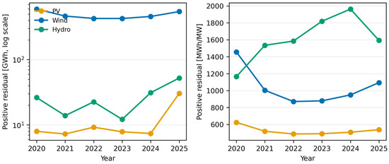
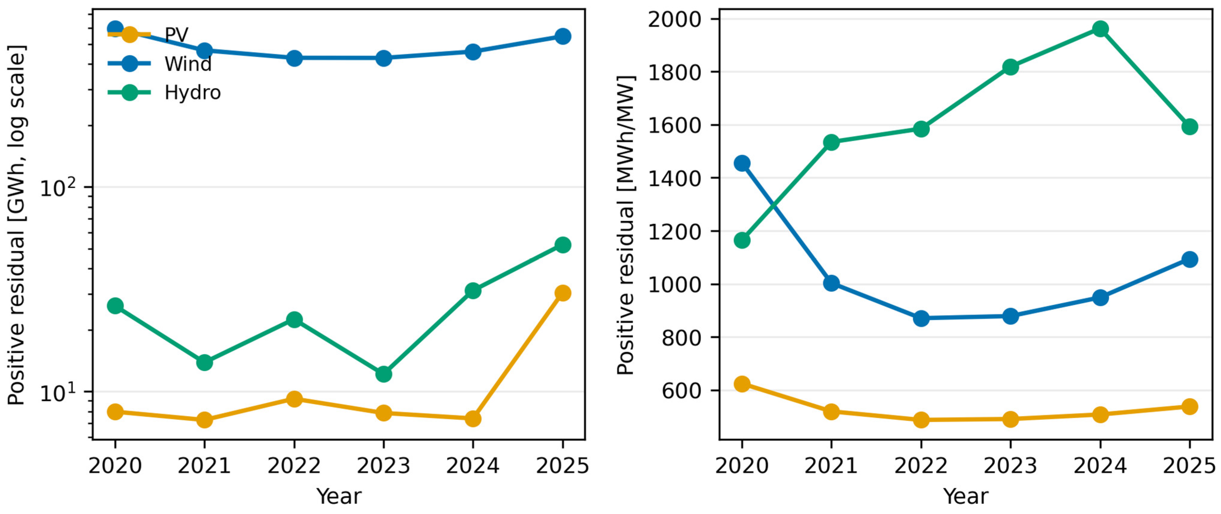
The annual positive residual differs by orders of magnitude between technologies (Figure 2 and Table 6). Wind has the largest absolute residual in every year, but the capacity-normalised view changes the comparison. In 2025, positive residuals equal 30.401 GWh for PV, 544.854 GWh for wind and 52.253 GWh for hydropower. The corresponding values per recorded megawatt are 538.3, 1094.2 and 1592.4 MWh/MW. The 2025 increase in PV residual coincides with an increase in recorded PV capacity from 14.530 MW in 2024 to 56.475 MW in 2025, illustrating why absolute values should not be interpreted without the denominator.

Figure 2. Annual positive model-to-meter residual by technology: absolute values on a logarithmic scale (left) and capacity-normalised values (right). The metric is not operator-confirmed curtailment.

Table 6. Annual positive model-to-meter residual in absolute and capacity-normalised form.

Year	PV [GWh]	PV [MWh/MW]	Wind [GWh]	Wind [MWh/MW]	Hydro [GWh]	Hydro [MWh/MW]
2020	7.968	624.8	595.648	1456.3	26.244	1164.7
2021	7.262	519.9	465.408	1003.3	13.872	1534.8
2022	9.218	487.8	427.784	871.0	22.558	1584.7
2023	7.851	491.2	427.331	878.9	12.168	1818.6
2024	7.384	508.2	458.919	949.1	31.179	1962.5
2025	30.401	538.3	544.854	1094.2	52.253	1592.4

3.2. Charging Outcomes in 2025

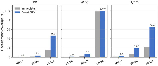
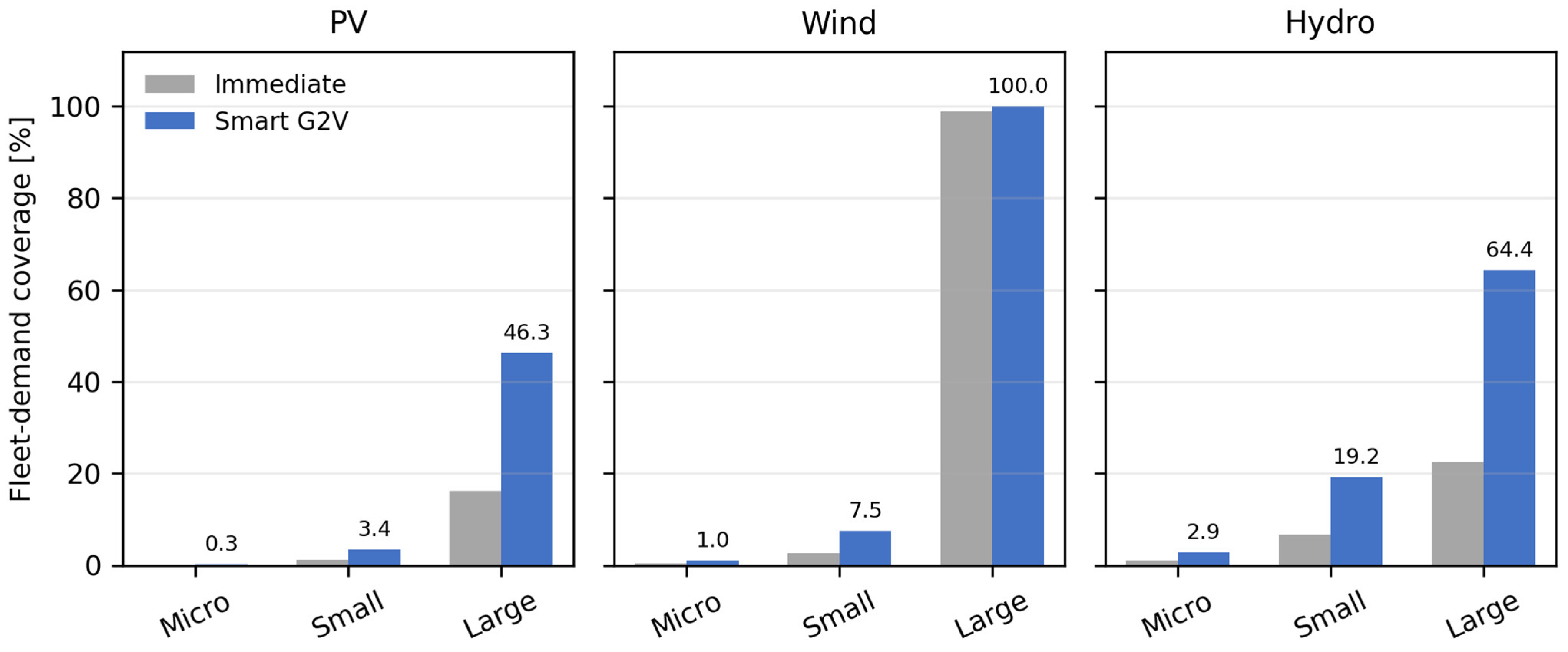
Table 7 reports the corrected 2025 single-pool results. Micro and small sources offer too little residual energy to cover a large share of annual fleet demand. Smart-G2V coverage in the micro class ranges from 0.29% for PV to 2.89% for hydropower; in the small class it ranges from 3.43% for PV to 19.22% for hydropower. Because demand does not bind in those cases, all energy that passes the simplified accessibility screen is assigned to Smart G2V.

Table 7. Corrected single-pool results for 2025. Energy values are annual. “Accessible” is the sum of C_m,k,y,c; utilisation is Smart G2V divided by accessible energy.

Tech.	Class	n	P [MW]	G+ [GWh]	C [GWh]	I [GWh]	S [GWh]	Coverage I→S [%]	Util. S [%]
PV	Micro	77	0.587	0.174	0.157	0.055	0.157	0.10 → 0.29	100.00
PV	Small	18	2.615	2.073	1.866	0.653	1.866	1.20 → 3.43	100.00
PV	Large	15	53.273	28.153	25.185	8.815	25.185	16.21 → 46.31	100.00
Wind	Micro	38	0.317	0.606	0.546	0.191	0.546	0.35 → 1.00	100.00
Wind	Small	8	2.375	4.514	4.062	1.422	4.062	2.61 → 7.47	100.00
Wind	Large	32	495.260	539.734	249.660	53.829	54.389	98.97 → 100.00	21.79
Hydro	Micro	55	1.610	1.744	1.570	0.550	1.570	1.01 → 2.89	100.00
Hydro	Small	26	5.894	11.612	10.451	3.658	10.451	6.73 → 19.22	100.00
Hydro	Large	9	25.310	38.897	35.007	12.252	35.007	22.53 → 64.36	100.00

The large-source class differentiates the technologies (Figure 3). PV provides 25.185 GWh of accessible energy and 46.31% Smart-G2V coverage, compared with 16.21% under immediate charging. Hydropower provides 35.007 GWh and 64.36% Smart-G2V coverage, compared with 22.53% under immediate charging. For wind, the power/window constraint admits 249.660 GWh, much more than the 54.389 GWh fleet demand. Smart G2V therefore reaches 100% coverage, while immediate charging already reaches 98.97% because many model-level demand caps bind even at the assumed 35% overlap. The near equality of the two wind modes follows from the size of the accessible pool. Immediate charging assigns min(ρ C_m, d_m). For a large share of models, ρ × 249.660 GWh already exceeds model demand, so min(ρ C_m, d_m) = d_m, and immediate charging converges on Smart G2V. The 2.857-fold ratio appears only in the unsaturated PV and hydropower cases: 46.31/16.21 = 2.857 and 64.36/22.53 = 2.857. Annual coverage of 100% for wind is energy sufficiency under the assumed window. It is not evidence that charging and wind production coincide in any hour.

Figure 3. Immediate and Smart-G2V coverage of annual sample demand in the 2025 capacity classes. Labels above the blue bars show Smart-G2V coverage.

Wind’s 100% demand coverage must not be confused with full use of the accessible residual. Only 21.79% of the 249.660 GWh accessible amount is assigned to mobility demand; the remainder is left unused by the annual charging model. By contrast, PV and hydropower large-source scenarios use 100% of the accessible amount because demand remains unsatisfied.

3.3. Interannual Results for Large Sources

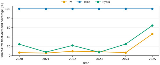
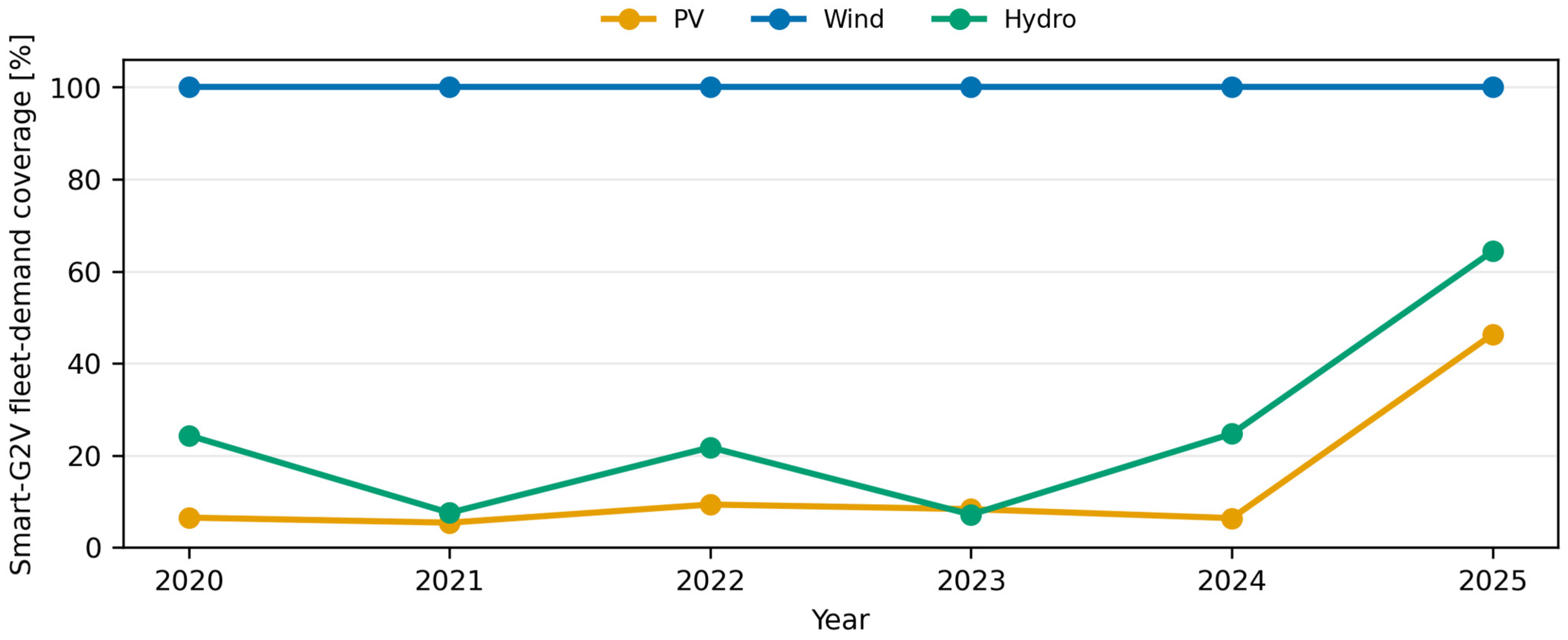
The large wind class reaches 100% Smart-G2V coverage in every study year because the simplified power/window limit, although binding, still admits more energy than annual fleet demand (Figure 4). PV large-source coverage is between 5.37% and 9.32% in 2020–2024 before increasing to 46.31% in 2025. Hydropower is more variable: coverage is 7.14–24.69% in 2020–2024 and 64.36% in 2025. The pattern follows the input residual and recorded-capacity panels; it is not an estimated causal time trend.

Figure 4. Smart-G2V coverage of annual sample demand in the large-source class, 2020–2025.

3.4. Binding Constraints and Sensitivity

At baseline, the positive-residual energy limit binds for all PV and hydropower capacity classes and for micro and small wind. The power/window constraint binds for large wind. In that scenario a second constraint—the EV-demand cap—then limits Smart-G2V uptake. Large PV is also marginally affected by the power/window constraint at some model rows, which is why accessible energy (25.185 GWh) is slightly below 0.9 × 28.153 = 25.338 GWh.

Reducing α from 0.90 to 0.70 lowers Smart-G2V coverage from 46.31% to 36.15% for PV and from 64.36% to 50.06% for hydropower; wind remains at 100% because accessible energy still exceeds demand. Raising α to 1.00 produces 51.35% PV coverage and 71.52% hydropower coverage. The overlap factor changes only the immediate strategy. At ρ = 0.20, immediate coverage is 9.26%, 87.45% and 12.87% for PV, wind and hydropower, respectively; at ρ = 0.50, the values are 23.15%, 99.56% and 32.18%. Table 3 reports coverage. The corresponding Smart-G2V utilisation of accessible energy stays at 100% for large PV and hydropower in every listed row, because demand remains unmet, and at 21.79% for large wind at the 100 MW and 150 MW ceilings, because demand saturates first. At 50 MW, the wind coverage falls to 99.56%, so utilisation of the reduced accessible pool is effectively complete. The availability–window product is 0.25 × 6 = 1.5 h/day for PV and 0.60 × 12 = 7.2 h/day for wind and hydropower, a factor of 4.8. That product, not residual size alone, sets the power/window ranking. One-at-a-time variation does not trace this interaction; the analytical product is reported here because the released files do not support a joint hourly redesign.

Connection capacity matters most where the power/window constraint binds. At 50 MW, Smart-G2V coverage is 43.08% for PV and 99.56% for wind; at 150 MW, it is 46.58% and 100%, respectively. Hydropower remains at 64.36% because its 2025 large-source result is energy-limited under all three connection settings. These stress tests confirm that the apparent technology ranking is conditional on both the residual input and the technology-specific availability/window assumptions.

3.5. V2G Capacity Envelope

Four model labels—Tesla Model 3 and Tesla Model Y (Tesla, Inc., Austin, TX, USA), Nissan Leaf 40 kWh (Nissan Motor Co., Ltd., Yokohama, Japan) and Kia EV6 (Kia Corporation, Seoul, Republic of Korea)—carry χ_m = 1 in the input matrix. They represent 7109 vehicles, or 35.47% of the analytical sample. With β = 0.40, a 20–80% SOC window and η_dis = 0.90, the resulting energy envelope is 112.929 MWh on the battery side and 101.636 MWh on the grid side per assumed event. Multiplication by 0.25 equivalent events/day gives a purely theoretical annual grid-side throughput ceiling of 9.274 GWh.

This number is deliberately not reported by technology or added to the Smart-G2V utilisation ratio. The annual RES data contain no deficit-period timestamps against which discharge could be scheduled. Moreover, the model-level eligibility flag does not verify every registered vehicle’s trim, production year, charger, protocol implementation or market approval. The envelope is therefore a scale indicator for a subsequent time-series study, not evidence that 9.274 GWh/year can be exported.

3.6. Calculation Quality Controls

The corrected matrix satisfies its algebraic invariants. This confirms reproducibility of the stated annual model, but it does not validate the behavioural assumptions or the physical meaning of the positive residual. Those require external data and a higher-resolution design.

4. Discussion

4.1. Answers to the Research Questions

First, the supplied annual positive residuals differ greatly across technology, year and capacity class. Absolute wind values dominate because recorded wind capacity is much larger, while hydropower often has the largest residual per recorded megawatt. Normalisation is therefore necessary, but even a normalised residual remains a model-to-meter difference rather than verified curtailment.

Second, Smart G2V provides the largest relative gain over immediate charging when accessible residual energy is below demand and the overlap factor is low. In the 2025 large PV and hydropower cases, coordinated uptake approximately triples the amount assigned relative to the 35% overlap baseline. This direction agrees with time-resolved studies showing that flexible charging can reduce renewable spillage or improve integration [6,7,8,9]. The present magnitudes are not directly comparable because the annual screen assumes that energy can be shifted within a technology-specific window without reconstructing chronology.

Third, constraint order matters. Wind has a very large positive residual, but the connection/window calculation limits accessible energy to 249.660 GWh. EV demand then becomes the binding cap for Smart G2V, leaving 78.21% of accessible energy unused. This result supports the broader literature’s conclusion that charging flexibility should be analysed jointly with network capacity and system operation [20,22], rather than inferred from an annual surplus alone.

Fourth, the V2G calculation supports only a capacity envelope. The separation from Smart-G2V utilisation avoids an accounting error in which discharge is treated as additional absorption of renewable energy. Operational V2G would require both a prior charging path and a later grid need. Hardware efficiency [23], battery wear and compensation [24], interoperability [25,26] and user availability would all reduce or reshape the deliverable service.

4.2. Interpretation for DSO and Charging-Infrastructure Planning

The screen can help rank combinations for further study. A high positive residual, adequate connection headroom and a sizable EV demand pool identify scenarios in which timestamped analysis is worthwhile. Low annual coverage in the micro PV case does not imply that local PV–EV coupling is ineffective; it indicates that the aggregated positive residual in that class is small relative to the chosen fleet. Conversely, 100% wind coverage does not imply that wind energy can physically charge every vehicle, because neither co-location nor temporal coincidence is established.

For DSO planning, the appropriate next step is to link source records to feeder or substation topology, replace the common 100 MW connection assumption with site-specific export/import limits and represent charger locations. The present proportional allocation is neutral and reproducible, but an operational model could prioritize vehicles by departure time, price, network constraint, emissions or fairness. It could also redistribute unused energy after an individual model reaches its demand cap.

4.3. Why the Residual Must Not Be Called Curtailment

Curtailment normally refers to otherwise available generation that is deliberately reduced because of system, market or plant constraints [1,2]. An annual benchmark error cannot distinguish that mechanism from resource forecast error, outage, maintenance, inverter availability, measurement alignment or a change in the asset population. The authentic provenance of the supplied DSO records strengthens traceability; it does not change the identification problem.

A future curtailment study should include at least a time-indexed unconstrained-production estimate, metered output, dispatch or redispatch flags, plant availability, grid-constraint location and consistent asset identifiers. The current result should instead be read as the maximum annual EV-demand match under a specified counterfactual availability fraction. This narrower wording is central to the validity of the paper.

4.4. Smart G2V Before V2G

The results support a deployment sequence in which unidirectional smart charging is assessed before bidirectional export. Smart G2V can shift an existing mobility load and avoids additional battery discharge. International guidance similarly treats managed charging as a foundational flexibility resource [25,35]. V2G may add value when the grid needs energy or ancillary services, but it requires a more demanding chain of verified vehicle, charger, communication and market compatibility [19,23,24,25,26].

The fixed 90% charging and 90% discharge efficiencies are convenient screening values. Measurements show that actual efficiency depends on power and hardware [23,31,32]. A high annual throughput cap should therefore not be monetized without an efficiency map, degradation model, availability distribution and service-specific dispatch. The reported 9.274 GWh/year is an upper throughput assumption, not revenue-bearing energy.

4.5. Limitations

The study has the following limitations.

• Annual aggregation removes the temporal coincidence needed to demonstrate charging feasibility or curtailment reduction. The daily windows are scalar energy constraints, not reconstructed time series.
• RES data were supplied by a DSO, but plant output was not independently re-measured, and the meaning of every modelled-energy field could not be verified against operator event logs. The installation panel changes across years.
• Twenty-six hydropower rows lack capacity. Their zero energy means they do not affect energy results, but they remain part of record counts and cannot contribute to capacity-normalised denominators.
• The 30-model, 20,043-vehicle CEPiK extract is a supplier-provided analytical sample, not the entire national fleet. Model labels may pool multiple variants.
• A common 15,000 km/year is assumed. PHEVs are treated as if all kilometres were electric; no observed PHEV utility factor is available.
• One representative consumption profile is assigned to each model. Catalogue or normalized consumption does not capture speed, temperature, heating/cooling, payload, battery ageing or driver heterogeneity [33,34].
• Vehicle availability, charging window, capturable fraction, overlap, connection power and participation are deterministic assumptions. The sensitivity analysis is structural and does not provide probabilistic uncertainty.
• The proportional allocation is not an optimization, and unused energy is not redistributed after model-level saturation.
• No feeder topology, voltage, thermal loading, losses, co-location, market price, emissions intensity, other electrical load or competing flexibility resource is represented.
• V2G eligibility is a model-level input flag and is not verified at the level of trim, model year, charger, protocol, warranty, regulation or user contract. The battery-capacity input is not independently classified as gross or usable. SOC dynamics, charging replenishment and degradation costs are absent.

These limitations constrain the claim to a conditional annual screen. They do not invalidate the arithmetic, but they preclude statements about actual curtailment avoided, feeder security, economic benefit or deliverable V2G service.

4.6. Further Work

The first extension should use 15 min or hourly DSO data with consistent plant identifiers and explicit unconstrained-production or constraint-event information. A rolling-horizon scheduler could then enforce arrival, departure, SOC, charger power, bidirectional efficiency and a terminal SOC requirement. The second extension should map RES sites and charging demand to substations or feeders and solve a network-constrained optimal power-flow or hosting-capacity problem. The third should use stochastic or empirically estimated distributions for travel, plug-in time and willingness to participate. Finally, a V2G module should include cycle- and calendar-ageing costs, service prices, warranty constraints, protocol verification and sensitivity to the participating fleet share. Neighbouring network studies already optimise wind uncertainty in power flow [36] and the joint siting of charging stations with distributed generators [37]. Both require topology that these annual records do not contain, so they bound the next step rather than the present screen.

5. Conclusions

This study revised an annual EV–RES matching calculation into a consistent single-pool screening model. The main findings are as follows: They separate outcomes imposed by the stated assumptions from findings that would require independent validation.

• The registration-weighted 30-model sample represents 20,043 vehicles and has a source-side annual charging demand of 54.389 GWh under the stated consumption, distance and efficiency assumptions.
• In 2025, large-source Smart-G2V coverage is 46.31% for PV, 64.36% for hydropower and 100.00% for wind, compared with 16.21%, 22.53% and 98.97% for immediate charging. The 2.857-fold ratio in the unsaturated cases is 1/ρ at ρ = 0.35; it is not an independent empirical finding.
• Large wind is power/window limited before it becomes EV-demand limited. It provides 249.660 GWh of technically accessible energy, but only 54.389 GWh is assigned, giving 21.79% utilisation. Coverage of 100% is annual sufficiency, not hourly feasibility.
• The eligibility-filtered V2G envelope is 101.636 MWh per event and 9.274 GWh/year under the assumed equivalent-cycle cap. It is hypothetical, is not added to RES utilisation and is not claimed as verified export.
• The positive model-to-meter residual is not verified curtailment. High-frequency production, availability, network and charging data are necessary before operational or economic conclusions can be drawn.

The resulting model is suitable for transparent pre-feasibility screening and for selecting cases that merit detailed simulation. Its scientific value depends on preserving the narrow scope of these conclusions.

References

- Bird, L.; Lew, D.; Milligan, M.; Carlini, E.M.; Estanqueiro, A.; Flynn, D.; Gómez-Lázaro, E.; Holttinen, H.; Menemenlis, N.; Orths, A.; et al. Wind and solar energy curtailment: A review of international experience. Renew. Sustain. Energy Rev. 2016, 65, 577–586. [Google Scholar] [CrossRef] [Scilit]
- O’Shaughnessy, E.; Cruce, J.; Xu, K. Too much of a good thing? Global trends in the curtailment of solar PV. Sol. Energy 2020, 208, 1068–1077. [Google Scholar] [CrossRef] [Scilit] [PubMed]
- Lund, P.D.; Lindgren, J.; Mikkola, J.; Salpakari, J. Review of energy system flexibility measures to enable high levels of variable renewable electricity. Renew. Sustain. Energy Rev. 2015, 45, 785–807. [Google Scholar] [CrossRef] [Scilit]
- Brown, T.; Schlachtberger, D.; Kies, A.; Schramm, S.; Greiner, M. Synergies of sector coupling and transmission reinforcement in a cost-optimised, highly renewable European energy system. Energy 2018, 160, 720–739. [Google Scholar] [CrossRef] [Scilit]
- Denholm, P.; Hand, M. Grid flexibility and storage required to achieve very high penetration of variable renewable electricity. Energy Policy 2011, 39, 1817–1830. [Google Scholar] [CrossRef] [Scilit]
- Szinai, J.K.; Sheppard, C.J.R.; Abhyankar, N.; Gopal, A.R. Reduced grid operating costs and renewable energy curtailment with electric vehicle charge management. Energy Policy 2020, 136, 111051. [Google Scholar] [CrossRef] [Scilit]
- Dixon, J.; Bukhsh, W.; Edmunds, C.; Bell, K. Scheduling electric vehicle charging to minimise carbon emissions and wind curtailment. Renew. Energy 2020, 161, 1072–1091. [Google Scholar] [CrossRef] [Scilit]
- Saadatmandi, S.; Chicco, G.; Favenza, A.; Mozzato, A.; Giordano, F.; Arnone, M. Smart electric vehicle charging for reducing photovoltaic energy curtailment. Electr. Power Syst. Res. 2024, 230, 110181. [Google Scholar] [CrossRef] [Scilit]
- Xu, R.; Seatle, M.; Kennedy, C.; McPherson, M. Flexible electric vehicle charging and its role in variable renewable energy integration. Environ. Syst. Res. 2023, 12, 11. [Google Scholar] [CrossRef] [Scilit]
- Richardson, D.B. Electric vehicles and the electric grid: A review of modeling approaches, impacts, and renewable energy integration. Renew. Sustain. Energy Rev. 2013, 19, 247–254. [Google Scholar] [CrossRef] [Scilit]
- Mwasilu, F.; Justo, J.J.; Kim, E.-K.; Do, T.D.; Jung, J.-W. Electric vehicles and smart grid interaction: A review on vehicle to grid and renewable energy sources integration. Renew. Sustain. Energy Rev. 2014, 34, 501–516. [Google Scholar] [CrossRef] [Scilit]
- Sadeghian, O.; Oshnoei, A.; Mohammadi-Ivatloo, B.; Vahidinasab, V.; Anvari-Moghaddam, A. A comprehensive review on electric vehicles smart charging: Solutions, strategies, technologies, and challenges. J. Energy Storage 2022, 54, 105241. [Google Scholar] [CrossRef] [Scilit]
- Barman, P.; Dutta, L.; Bordoloi, S.; Kalita, A.; Buragohain, P.; Bharali, S.; Azzopardi, B. Renewable energy integration with electric vehicle technology: A review of the existing smart charging approaches. Renew. Sustain. Energy Rev. 2023, 183, 113518. [Google Scholar] [CrossRef] [Scilit]
- Muratori, M. Impact of uncoordinated plug-in electric vehicle charging on residential power demand. Nat. Energy 2018, 3, 193–201. [Google Scholar] [CrossRef] [Scilit]
- Heinisch, V.; Göransson, L.; Erlandsson, R.; Hodel, H.; Johnsson, F.; Odenberger, M. Smart electric vehicle charging strategies for sectoral coupling in a city energy system. Appl. Energy 2021, 288, 116640. [Google Scholar] [CrossRef] [Scilit]
- Gunkel, P.A.; Bergaentzlé, C.; Jensen, I.G.; Scheller, F. From passive to active: Flexibility from electric vehicles in the context of transmission system development. Appl. Energy 2020, 277, 115526. [Google Scholar] [CrossRef] [Scilit]
- Kempton, W.; Tomić, J. Vehicle-to-grid power fundamentals: Calculating capacity and net revenue. J. Power Sources 2005, 144, 268–279. [Google Scholar] [CrossRef] [Scilit]
- Lund, H.; Kempton, W. Integration of renewable energy into the transport and electricity sectors through V2G. Energy Policy 2008, 36, 3578–3587. [Google Scholar] [CrossRef] [Scilit]
- İnci, M.; Çelik, Ö.; Lashab, A.; Bayındır, K.Ç.; Vasquez, J.C.; Guerrero, J.M. Power system integration of electric vehicles: A review on impacts and contributions to the smart grid. Appl. Sci. 2024, 14, 2246. [Google Scholar] [CrossRef] [Scilit]
- Tayri, A.; Ma, X. Grid impacts of electric vehicle charging: A review of challenges and mitigation strategies. Energies 2025, 18, 3807. [Google Scholar] [CrossRef] [Scilit]
- Lee, H.; Kim, H.; Kim, H.; Kim, H. Optimal Vehicle-to-Grid charge scheduling for electric vehicles based on dynamic programming. Energies 2025, 18, 1109. [Google Scholar] [CrossRef] [Scilit]
- Stamatakis, D.; Tolis, A.I. Coordinated electric vehicle demand management in the unit commitment problem integrated with transmission constraints. Energies 2025, 18, 4293. [Google Scholar] [CrossRef] [Scilit]
- Sevdari, K.; Pedersen, K.L.; Fabbri, G.; Knudsen, R.M.; Alami, A.; Engelhardt, J.; Marinelli, M. Efficiency of bidirectional EV charging: Key insights from implementing ISO 15118-20 CCS2 and CHAdeMO. Sustain. Energy Technol. Assess. 2025, 83, 104654. [Google Scholar] [CrossRef] [Scilit]
- Sagaria, S.; van der Kam, M.; Boström, T. Vehicle-to-grid impact on battery degradation and estimation of V2G economic compensation. Appl. Energy 2025, 377, 124546. [Google Scholar] [CrossRef] [Scilit]
- International Energy Agency. Vehicle-to-Grid Technology; IEA: Paris, France, 2026. Available online: https://www.iea.org/reports/vehicle-to-grid-technology (accessed on 15 September 2026).
- ISO 15118-20:2022; Road Vehicles—Vehicle to Grid Communication Interface—Part 20: 2nd Generation Network Layer and Application Layer Requirements. ISO: Geneva, Switzerland, 2022. Available online: https://www.iso.org/standard/77845.html (accessed on 15 September 2026).
- Central Register of Vehicles and Drivers. CEPiK Portal and API Information. Available online: https://www.gov.pl/web/cepik (accessed on 15 September 2026).
- European Parliament and Council. Regulation (EU) 2023/1804 of 13 September 2023 on the deployment of alternative fuels infrastructure, and repealing Directive 2014/94/EU. Off. J. Eur. Union 2023, L 234, 1–47. [Google Scholar]
- Radović, U. Effects of electric vehicles on the Polish power generation system, emissions of CO2 and other air pollutants. Zesz. Nauk. Inst. Gospod. Surowcami Miner. Energią PAN 2018, 104, 69–84. [Google Scholar] [CrossRef] [PubMed]
- Lula, A.; Zagrajek, K. A concept of using a private electric vehicle to optimize the costs of electricity in household equipped with a PV power plant. Prz. Elektrotech. 2022, 98, 7–14. [Google Scholar] [CrossRef] [Scilit]
- Reick, B.; Konzept, A.; Kaufmann, A.; Stetter, R.; Engelmann, D. Influence of charging losses on energy consumption and CO2 emissions of battery-electric vehicles. Vehicles 2021, 3, 736–748. [Google Scholar] [CrossRef] [Scilit]
- Apostolaki-Iosifidou, E.; Codani, P.; Kempton, W. Measurement of power loss during electric vehicle charging and discharging. Energy 2017, 127, 730–742. [Google Scholar] [CrossRef] [Scilit]
- Seo, J.; Cha, J. Real-world analysis of energy consumption in a battery electric vehicle: Effects of ambient temperatures and thermal management system operation. Energy Convers. Manag. 2025, 345, 120372. [Google Scholar] [CrossRef] [Scilit]
- EV Database. Energy Consumption of Electric Vehicles. Available online: https://ev-database.org/cheatsheet/energy-consumption-electric-car (accessed on 15 September 2026).
- International Renewable Energy Agency. Innovation Outlook: Smart Charging for Electric Vehicles; IRENA: Abu Dhabi, United Arab Emirates, 2019. [Google Scholar]
- Albalawi, H.; Muhammad, Y.; Wadood, A.; Khan, B.S.; Zainab, S.T.; Alatwi, A.M. Leveraging the Performance of Integrated Power Systems with Wind Uncertainty Using Fractional Computing-Based Hybrid Method. Fractal Fract. 2024, 8, 532. [Google Scholar] [CrossRef] [Scilit]
- Alatwi, A.M.; Albalawi, H.; Wadood, A.; Atawi, I.E.; Alatawi, K.S.S. Novel GBest–Lévy Adaptive Differential Ant Bee Colony Optimization for Optimal Allocation of Electric Vehicle Charging Stations and Distributed Generators in Smart Distribution Systems. Energies 2025, 18, 6018. [Google Scholar] [CrossRef] [Scilit]
Disclaimer/Publisher’s Note: The statements, opinions and data contained in all publications are solely those of the individual author(s) and contributor(s) and not of MDPI and/or the editor(s). MDPI and/or the editor(s) disclaim responsibility for any injury to people or property resulting from any ideas, methods, instructions or products referred to in the content. |
© 2026 by the authors. Licensee MDPI, Basel, Switzerland. This article is an open access article distributed under the terms and conditions of the Creative Commons Attribution (CC BY) license.