The Main Control Factors and Productivity Evaluation Method of Stimulated Well Production Based on an Interpretable Machine Learning Model

Abstract

Low-permeability waterflooding reservoirs face numerous challenges, including low productivity per well, inadequate formation pressure maintenance, poor waterflood response, and low water injection utilization efficiency. Illustrated by Bai 153 Block in the Changqing Oilfield, the primary concern has shifted in recent years from fracture water breakthrough to formation blockages. Currently, low-yield wells (≤0.5 t) constitute a significant proportion (27.5%), with a recovery factor of only 0.41%. The effectiveness of stimulation treatments is influenced by reservoir properties, treatment types, process parameters, and production performance. Selecting candidate wells requires collecting and analyzing data such as individual well block characteristics. Evaluating treatment effectiveness involves substantial effort and complexity. Early fracturing treatments exhibited significant variations in effectiveness, and the primary controlling factors influencing fracturing success remained unclear. This paper proposes a big data analysis-based method for evaluating stimulation effectiveness in low-permeability waterflooding reservoirs. Utilizing preprocessed geological, construction, and production data from the target block, an integrated application of the Random Forest algorithm and Recursive Feature Elimination ranks the importance of factors affecting treatments and identifies the block’s main controlling factors. Using these factors as target parameters, a multivariate quantitative evaluation model for fracturing effectiveness is established. This model employs the Pearson correlation coefficient method, Recursive Feature Elimination, and the Random Forest algorithm. Results from the quantitative model indicate that the primary main controlling factors that significantly affect post-fracturing oil increment are production parameters, geological parameters such as vertical thickness, fracture pressure, and oil saturation; engineering parameters such as sand ratio, blowout volume, and fracturing method; and production parameters such as pre-measure cumulative fluid production, production months, and pre-measure cumulative oil production, which are most closely related to post-fracturing oil increment. These parameters show the strongest correlation with incremental oil production. The constructed quantitative model demonstrates a linear correlation rate exceeding 85% between predicted fracturing stimulation and actual well test production, verifying its validity. This approach provides a novel method and theoretical foundation for the post-evaluation of oil increment effectiveness from stimulation treatments in low-permeability waterflooding reservoirs.

1. Introduction

As a significant unconventional oil and gas resource, tight oil has garnered widespread attention owing to its substantial reserves and production potential [1]. However, the application of conventional hydraulic fracturing technology in this region has yielded suboptimal outcomes, primarily attributed to the lack of reservoir-specific fracturing designs and insufficient consideration of geological variations under differing reservoir conditions [2]. Consequently, substantial variations exist in post-fracturing well performance, significantly compromising the productivity and economic viability of tight oil wells. Therefore, it is imperative to analyze the primary controlling factors governing tight oil well productivity in this region. Based on this analysis, accurate prediction of well productivity is essential to provide a foundation for optimizing fracturing designs.

The development of tight oil wells is characterized by significant complexity and uncertainty due to the influence of geological, engineering, and other factors on well productivity [3]. Furthermore, the strong heterogeneity of regional tight oil reservoirs makes it challenging to identify the main controlling factors governing well productivity. Traditional methods for predicting well productivity often yield limited accuracy, and optimizing fracturing parameters is inherently complex due to the interplay of multiple factors [4]. Machine learning techniques are now widely applied to predict tight oil well productivity and optimize fracturing parameters. Among these, the Random Forest algorithm—a prevalent ensemble learning method—leverages geological, fracturing, and production data. It captures nonlinear relationships within the data by constructing multiple decision trees and aggregating their outputs (through voting or averaging). This approach effectively handles complex interactions to enhance productivity prediction accuracy and provides a scientific basis for fracturing parameter optimization [5].

Identifying the main controlling factors for tight reservoir fracturing treatments, conducting timely and systematic evaluations of the implementation effectiveness at each development stage, and guiding iterative design optimization are crucial for enhancing the recovery factor of tight reservoirs. Two primary methods exist for evaluating fracturing effectiveness: Direct Method: Evaluates the stimulated reservoir volume (SRV) created by large-scale fracturing through monitoring a certain number of fractures. Indirect Method: Employs mathematical approaches to assess fracturing effectiveness [6,7]. In actual production, numerous factors determine fracturing outcomes. For different fracturing designs, identifying the key influencing factors often requires detailed analysis. Consequently, researchers worldwide have increasingly applied machine learning methods to evaluate oil and gas field development effectiveness, yielding significant research results.

Leveraging various data mining and machine learning algorithms, many scholars have developed models mapping geological, engineering, and other characteristic variables to estimated ultimate recovery (EUR). Early research frequently employed traditional regression algorithms, such as multiple linear regression and ridge regression. These methods predicted EUR by establishing linear regression equations between characteristic variables (geological, engineering, etc.) and cumulative production. However, this approach fails to account for potential nonlinear relationships between the variables and EUR, introducing significant limitations. For instance, Al-Alwani et al. constructed three multiple linear regression models using data from 2700 Marcellus shale gas wells [8]. Their models used 10 numerical features—including total fluid volume, total proppant volume, perforated interval length, and shale content—as inputs to predict initial post-fracturing production, 12-month cumulative gas production, and 24-month cumulative gas production. Nevertheless, such regression algorithms struggle to handle nonlinear relationships effectively and require predefined functional forms, inevitably compromising prediction accuracy. Consequently, many researchers have increasingly focused on machine learning algorithms, which offer superior capability for capturing complex nonlinear mappings.

Neural networks are among the most widely used machine learning algorithms. Their flexible, modular architecture enables better adaptation to diverse static yield prediction tasks. A variety of neural network types, ranging from simple self-organizing maps (SOM) and backpropagation neural networks (BPNN) to more complex fuzzy neural networks (FNN), deep neural networks (DNN), and hybrid deep neural networks, have been successively applied. Oberwinkler et al. established a three-layer SOM model using data from 200 compact gas fracturing horizontal wells [9]. This model maps mixed-type features (numerical and categorical)—including reservoir thickness, prepad fluid volume, total sand volume, proppant type, and total fluid volume—to one-year cumulative gas production. Shelley et al. developed a model based on 301 fracturing wells, employing a feedforward neural network to map geological parameters (such as permeability, porosity, water saturation, and formation pressure) and engineering parameters (such as sanding intensity, fluid intensity, fracture spacing, and horizontal section length) to one-year cumulative oil production [10]. Stratton et al. constructed a DNN model with 4 hidden layers using data from 2061 Bakken shale oil wells [11]. The model predicts one-year barrel of oil equivalent (BOE) production post-fracturing but considers only numerical input features: reservoir thickness, fluid volume, sand volume, well depth, porosity, number of fracturing stages, and stage length. Wang et al. developed two DNN models, each with 3 hidden layers, based on data from 2919 Bakken shale oil fracturing wells [12]. These models predict 6-month and 18-month cumulative oil production after fracturing, respectively. The inputs comprise 11 numerical features and 7 categorical features related to wells, reservoirs, fractures, fracturing fluids, and proppants.

Beyond neural networks, algorithms including support vector machines (SVMs), Random Forest, and Gradient Boosting have also been applied to post-fracturing production prediction [13]. For example, Wang et al. utilized data from 4790 Canadian fracturing horizontal wells to establish and compare the predictive performance of Random Forest AdaBoost, SVM, and neural network models. Using 7 numerical features and 4 categorical features as inputs, their models predicted one-year post-fracturing barrel of oil equivalent (BOE) [14]. To further optimize model parameters and enhance prediction performance, machine learning models enhanced with hyperparameter tuning algorithms have been increasingly employed. For instance, Lu et al. used geological parameters—such as gas content, coal thickness, and temporary storage ratio—to develop a particle swarm optimization (PSO)-based SVM model for predicting the average daily production of coalbed methane wells [15]. Similarly, Akbari et al. applied a gray wolf optimizer (GWO)-enhanced SVM to predict the initial production of 34 fracturing wells in ultra-low permeability reservoirs [16].

Recurrent neural networks (RNNs) and their variants, such as LSTM and GRU, are valued for their memory capabilities and structural flexibility, making them commonly employed for multivariable time series prediction, including gas production forecasting [17,18]. Kanwal et al. developed an LSTM model using only production data to predict a single well’s cumulative gas output, demonstrating significantly better performance than ARIMA [19]. Similarly, Sun et al. found that an LSTM model incorporating tubing pressure as an exogenous variable yielded smaller errors than Arps decline analysis [20]. Lee et al. built an LSTM model for shale gas monthly production that accounted for well shut-in time, achieving higher accuracy than single-variable models [21]. Alimohammadi et al. compared LSTM, GRU, and BiRNN for single-step daily gas prediction, using tubing pressure and temperature as exogenous variables, and found GRU achieved the highest accuracy [22].

In practical applications, combining multiple models has proven more effective than using a single RNN or LSTM model alone for improving prediction accuracy. Among such hybrid approaches, integrating hyperparameter optimization algorithms with prediction models is the most common strategy. For instance, Song et al. utilized a Particle Swarm Optimization (PSO) algorithm to optimize an LSTM model, achieving higher accuracy for single-step daily production prediction in volcanic oil wells compared to Arps decline, RNN, and ARIMA models [23]. Liu et al. developed an LSTM model based on Ensemble Empirical Mode Decomposition (EEMD), incorporating tubing pressure and bottom hole temperature as exogenous variables [24]. The EEMD decomposed the time series production data into different modes, and a Genetic Algorithm (GA)-optimized LSTM was then used for single-step daily oil production prediction. Bao et al. employed Bayesian Optimization algorithms to optimize a combined Kalman Filter and LSTM model, establishing three distinct models for single-step prediction of daily oil production, cumulative oil production, and water cut [25]. This research demonstrates that combining models with hyperparameter optimization algorithms can significantly enhance prediction performance. However, it is noteworthy that these studies typically focus on multivariate, single-step prediction of post-pressure production dynamics.

The aforementioned research provides valuable methodological insights for this study. However, further investigation is warranted regarding the analysis of multi-factor coupling mechanisms and the enhancement of model generalization capabilities. Leveraging the static and dynamic reservoir data from the field, the introduction of machine learning algorithms to construct a fracturing performance evaluation model offers significant advantages. This approach enables both the rapid and accurate identification of the primary controlling factors influencing productivity and facilitates real-time optimization and adjustment of on-site fracturing parameters, thereby enhancing stimulation effectiveness. Focusing on the geological characteristics and development challenges of the Bai 153 Block in the Changqing Oilfield, this study leverages production well data following reservoir fracturing stimulation. Adopting an integrated geological-engineering analysis approach, we first characterize the reservoir geology and then evaluate post-fracturing productivity. Feature selection is performed using the Spearman correlation analysis method, while the primary geological and engineering factors controlling fracturing effectiveness are quantitatively evaluated through a combined application of Recursive Feature Elimination (RFE) and the Random Forest machine learning algorithm. This methodology provides theoretical support and practical guidance for subsequent well selection and optimization of on-site fracturing parameters, aiming to maximize productivity.

2. Data Processing and Quality Analysis

2.1. Data Acquisition

To evaluate the stimulation effectiveness of fracturing treatments in the Changqing Bai 153 well area, we utilize geological characteristics, completion parameters, and production data as the foundational dataset. Applying big data analytics, we identify the key factors influencing fracturing performance. During this analytical process, issues such as missing data, anomalies, and errors frequently arise. Consequently, comprehensive data quality assessment is required prior to modeling. Based on the assessment findings, data preprocessing—including imputation for missing values and correction of outliers—is essential to enhance data quality and ensure the reliability of the subsequent data mining results.

We have collected totally 380 fractured wells in the Changqing Bai 153 well area, the mean, variance, minimum, maximum, median, and quantile of characteristic parameters (geological factors, construction factors, production dynamic parameters before measures, and test production) were statistically analyzed. The distribution of characteristic parameters is shown in Table 1.

Table 1. Distribution of characteristic parameters.

Features	Abbreviation	Mean	Variance	Maximum	Median
Reservoir thickness	P1	10.7	11.4	43.2	9.3
Vertical thickness	P2	24.3	16.2	55.2	18.5
Resistivity	P3	21.3	20.2	89.4	26.25
Neutron	P4	40.9	17.8	173.55	36.41
Acoustic interval	P5	225.9	4.5	239.12	226.2
Porosity	P6	11.4	0.99	20.9	11.45
Permeability	P7	0.49	0.66	5.61	0.3
Oil saturation	P8	55.2	5.02	71.17	55.44
Clay content	P9	16.9	3.4	27.64	16.87
Acid amount	P10	1.58	3.14	20	1
Sand amount	P11	3.2	6.4	65	2.3
Sand ratio	P12	14.5	7.5	35	14.8
Fluid injection amount	P13	30.0	52.5	565.3	21
Pumping rate	P14	2.56	2.01	10	2.5
Breakdown pressure	P15	26.8	11.3	44	29.2
Working pressure	P16	24.6	10.0	43.5	27
Pumping-stop pressure	P17	13.0	4.9	30.3	14.1
Fracturing types	P18	-	-	-	-
Flowback volume	P19	84.6	58.6	283	76.5
initial daily liquid production	P20	2.34	1.34	8.97	1.98
Daily liquid production before stimulation	P21	1.04	0.64	4.92	1.01
Cumulative liquid production before stimulation	P22	3586.5	2503.1	11,965	3344
Production days	P23	1811.6	1263.7	4528.3	1933.45
Increase in oil production	P24	0.75	0.51	2.19	0.795

2.2. Data Preprocessing

2.2.1. Missing Value Processing

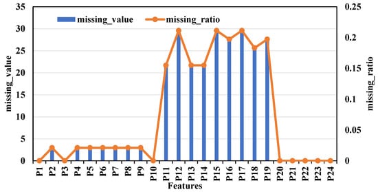
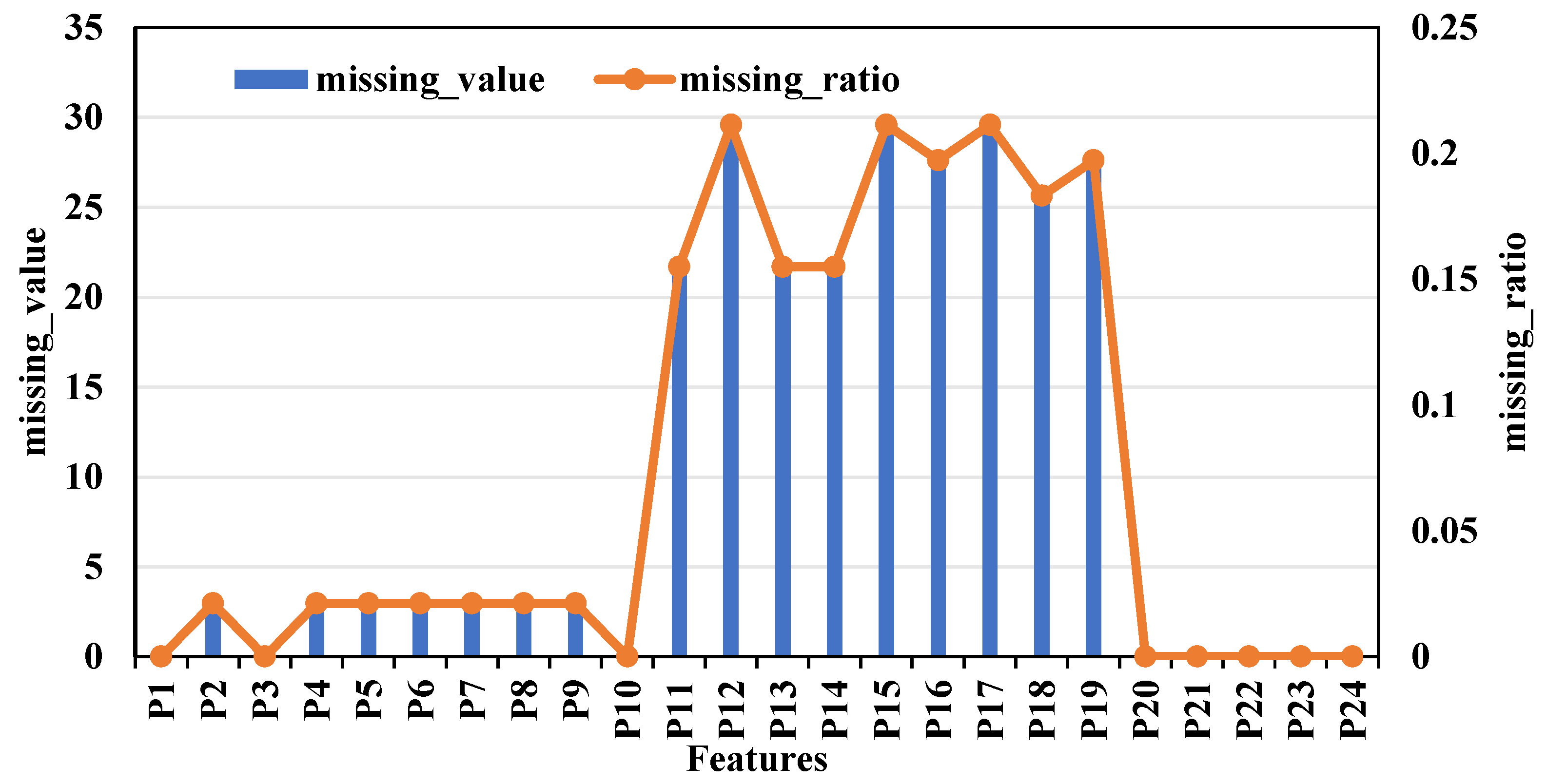
Feature parameter preprocessing primarily involves analyzing invalid and missing values. As illustrated in Figure 1, feature parameters become unusable for machine learning models when the proportion of missing values exceeds a certain threshold. This paper adopts the following principles for handling missing values: Exclude the attribute if the missing rate exceeds 40% and the attribute has low importance. Apply median imputation for attributes with a missing rate below 5%. Employ Random Forest multiple imputation for attributes with a missing rate above 5% and high importance. The Random Forest algorithm treats each feature with missing values as a function of the other features. It constructs a Random Forest model where the output of this function serves as an estimate, predicting missing data based on variable relationships. This approach yields more realistic imputed values. Figure 1 shows feature parameters with varying degrees of missingness. For example, the coal rock density has a missing rate of 7.3%. Given its relevance to adsorbed gas content (high importance), it cannot be simply excluded; therefore, Random Forest multiple imputation is applied. Conversely, attributes like reservoir pressure and perforation thickness, which have low missing rates, are suitable for direct median imputation.

Figure 1. Missing characteristic of fractured wells in Changqing Bai 153 well area.

2.2.2. Identification and Treatment of Outliers

Outliers, also known as isolated points, are extreme or unreasonable observations within a dataset. Statistically, they are defined as values deviating from the mean by more than twice the standard deviation; values exceeding three standard deviations are termed extreme outliers. To identify them, boxplots are utilized for each feature, flagging points outside the upper and lower whiskers as potential outliers. These flagged points are then cross-referenced with the original data records to distinguish and correct potential recording errors. However, outliers originating from excellent, poor, or experimental wells are retained. Subsequently, the Isolation Forest algorithm is employed to further detect outliers.

①

Box plot analysis

Sort all data by size, find the upper quartile (UQ) and lower quartile (LQ), calculate the difference IQR = UQ − LQ, and all data outside the range of [LQ − 1.5×IQR, UQ + 1.5×IQR] can be determined as outliers. The visualization method is to draw a box-whisker plot, box plot, or box-and-whisker plot for intuitive judgment. The box plot is used to statistically display the dispersion of a set of data and is mainly used to reflect the characteristics of the original data distribution. A box plot is a statistical chart used to display the distribution characteristics of data and identify outliers. By calculating quartiles and interquartile range (IQR), box plots can effectively detect outliers in data. The box diagram mainly consists of the following parts: ① Median, the median value of data that divides the data into two parts; ② First quartile (Q1), 25% percentile, indicating that 25% of the values in the data are less than or equal to Q1; ③ Third quartile (Q3), 75% percentile, indicating that 75% of the values in the data are less than or equal to Q3. Interquartile range (IQR), the difference between Q3 and Q1, used to measure the degree of data dispersion. The detection of outliers is based on Tukey’s Method. Mild outlier is located outside the inner limit (Q1 − 1.5×IQR to Q3 + 1.5×IQR) but within the outer limit (Q1 − 3×IQR to Q3 + 3×IQR). Extreme outlier is located outside the outer limit.

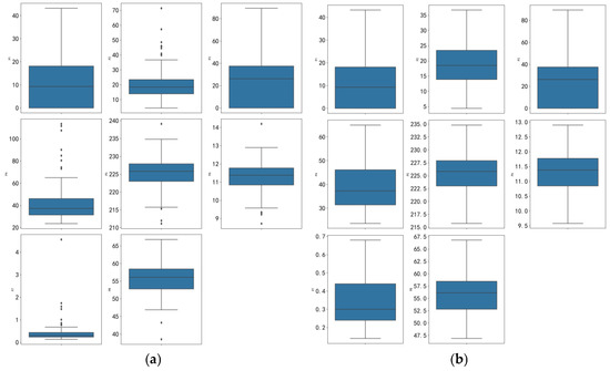
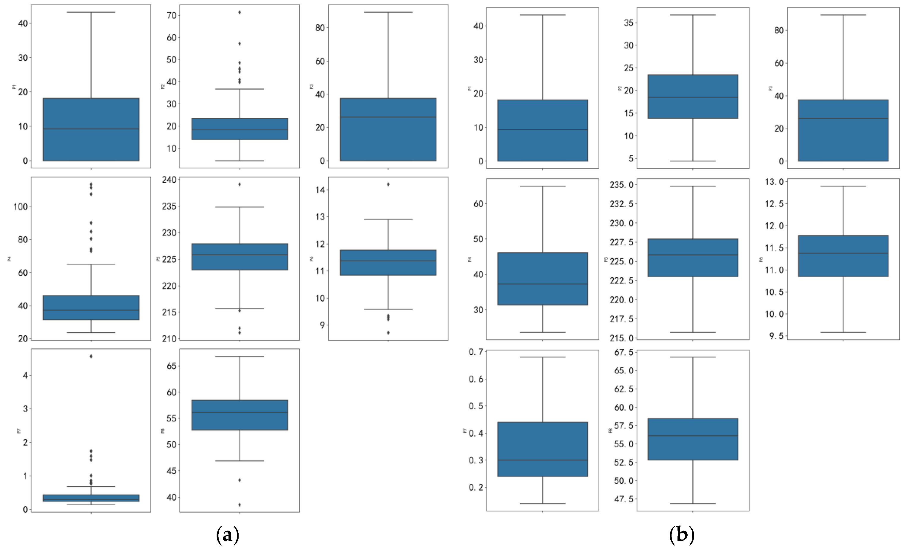
Figure 2a presents the box plot of selected geological and engineering parameters for the Linxing-Shenfu single-pressure single-production well straight well section prior to processing. Points lying outside the whiskers of this box plot represent outliers. Figure 2b displays the processed result, where these anomalous points have been adjusted to the respective whisker endpoints (i.e., the upper and lower whisker values of the box plot).

Figure 2. Box plot before and after processing some abnormal parameter values. (a) Before processing; (b) after processing.

Box plots are efficient and convenient for handling outliers. However, they have certain limitations. For some outliers, although they have a large gap with normal values, they are caused by special processes and do not violate technical mechanisms. Uniformly using box plots to handle outliers may accidentally delete representative special phenomena. Therefore, this article further adopts the Isolation Forest method to identify outliers.

②

Isolation Forest for Outlier Detection

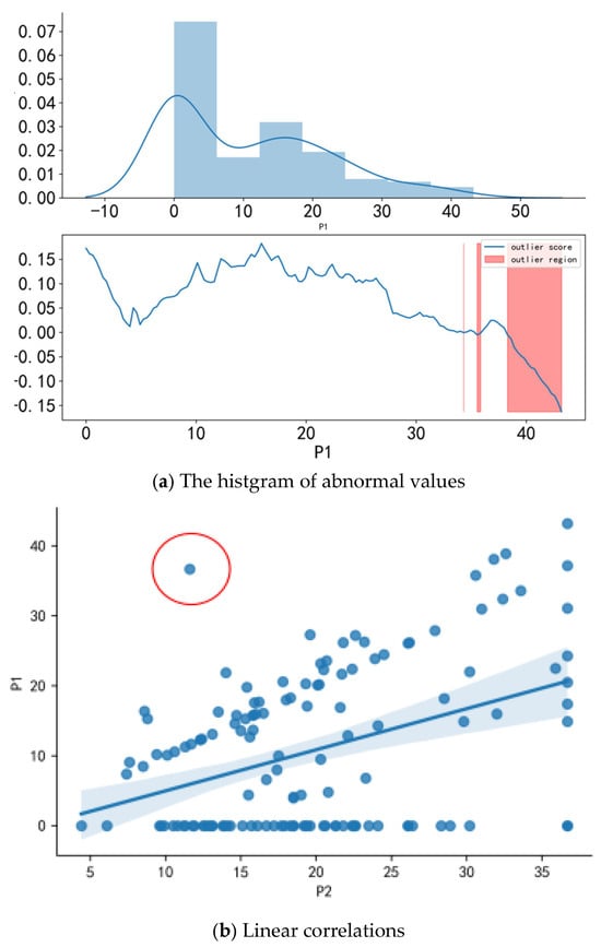
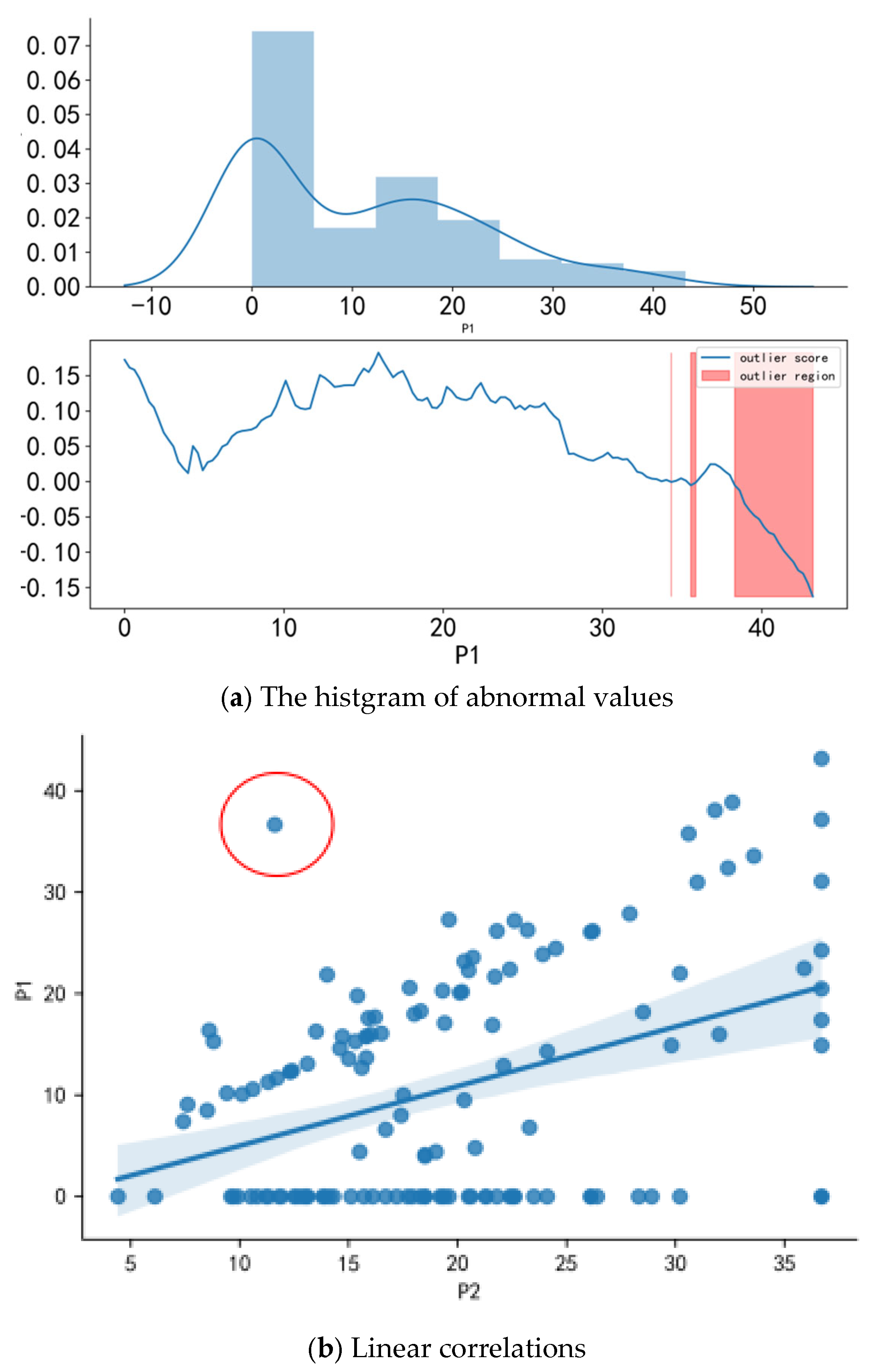
The Isolation Forest method recursively and randomly partitions the dataset until all sample points are isolated. Under this random partitioning strategy, outliers typically exhibit shorter path lengths to isolation. Intuitively, points in high-density clusters require more partitions to isolate, while low-density points are isolated more readily. Figure 3 presents the outliers identified by the Isolation Forest method for the feature variables. The upper panel displays the histogram and probability density function for a variable, which assesses its closeness to a normal distribution. For normally distributed data, the mean adequately represents the central tendency; for skewed distributions, the mode and median are more representative. The lower panel shows the anomaly scores assigned by the Isolation Forest algorithm across the variable’s range, where lower scores indicate a higher degree of outlierness. This visualization of univariate outlier identification highlights the outlier regions. The figure demonstrates that the anomaly scores align with the shape of the underlying distribution, with outlier regions corresponding to low-probability areas. This study employs the Python3.6 programming language and utilizes the Isolation Forest implementation within the Scikit-Learn library to identify outliers, with the contamination parameter set to 0.02. Using gas content and actual sand content as examples, Figure 3a displays the distribution regions (highlighted in red) identified as containing outliers by the Isolation Forest algorithm. By cross-referencing the original data files, gas content and actual sand content values within these regions can be flagged as outliers and adjusted. Figure 3b presents a bivariate linear relationship analysis. The discrete points circled in red appear sparse and distant from the high-density core population, further confirming their identification as outliers.

Figure 3. Isolated forest anomaly detection plot for single feature variable.

2.3. Feature Scaling

To address the challenges of handling multi-source heterogeneous features in high-dimensional data modeling, it is urgent to eliminate the feature weight bias caused by numerical dimensionality differences through feature standardization preprocessing. When there are orders of magnitude differences between feature dimensions, unstandardized Euclidean distance calculations will lead to severe bias towards large-scale feature parameters in modeling results. Therefore, two core algorithms, Min-Max Scaling and Z-score Scaling, are mainly used. The calculation formulas are shown in Equations (1) and (2), respectively:

$$\begin{array}{c}\stackrel{\mathrm{~}}{\mathit{x}} = {\displaystyle \frac{\mathit{x} -{\mathit{x}}_{\min }}{{\mathit{x}}_{\max } - {\mathit{x}}_{\min }}}\end{array}$$

(1)

$$\begin{array}{c}\stackrel{\mathrm{~}}{\mathit{x}}={\displaystyle \frac{\mathit{x}-\stackrel{\text{-}}{\mathit{x}}}{\mathsf{\sigma }}}\end{array}$$

(2)

Among them, $\mathrm{x}$ represents a certain feature, ${\mathrm{x}}_{\min }$, ${\mathrm{x}}_{\max }$, $\stackrel{\text{-}}{\mathrm{x}}$, $\mathsf{\sigma }$ are the minimum, maximum, mean, and variance of the feature in the training set, respectively, and represents the scaled feature. In addition, when the data distribution is very skewed, logarithmic transformation or square root transformation (when there are multiple 0 data values) can help stabilize the data distribution and make it closer to a normal distribution.

2.4. Feature Selection

The geological and engineering parameters comprise 28 feature variables, which may include irrelevant or redundant features. Feature selection addresses this by reducing the risk of overfitting, simplifying the data through dimensionality reduction, and enhancing model generalization. Additionally, this process improves model interpretability, deepens understanding of feature-value relationships, accelerates training, and typically improves model performance. Therefore, feature selection is generally employed to eliminate unnecessary redundant features.

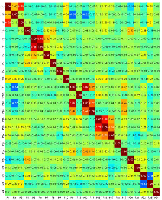
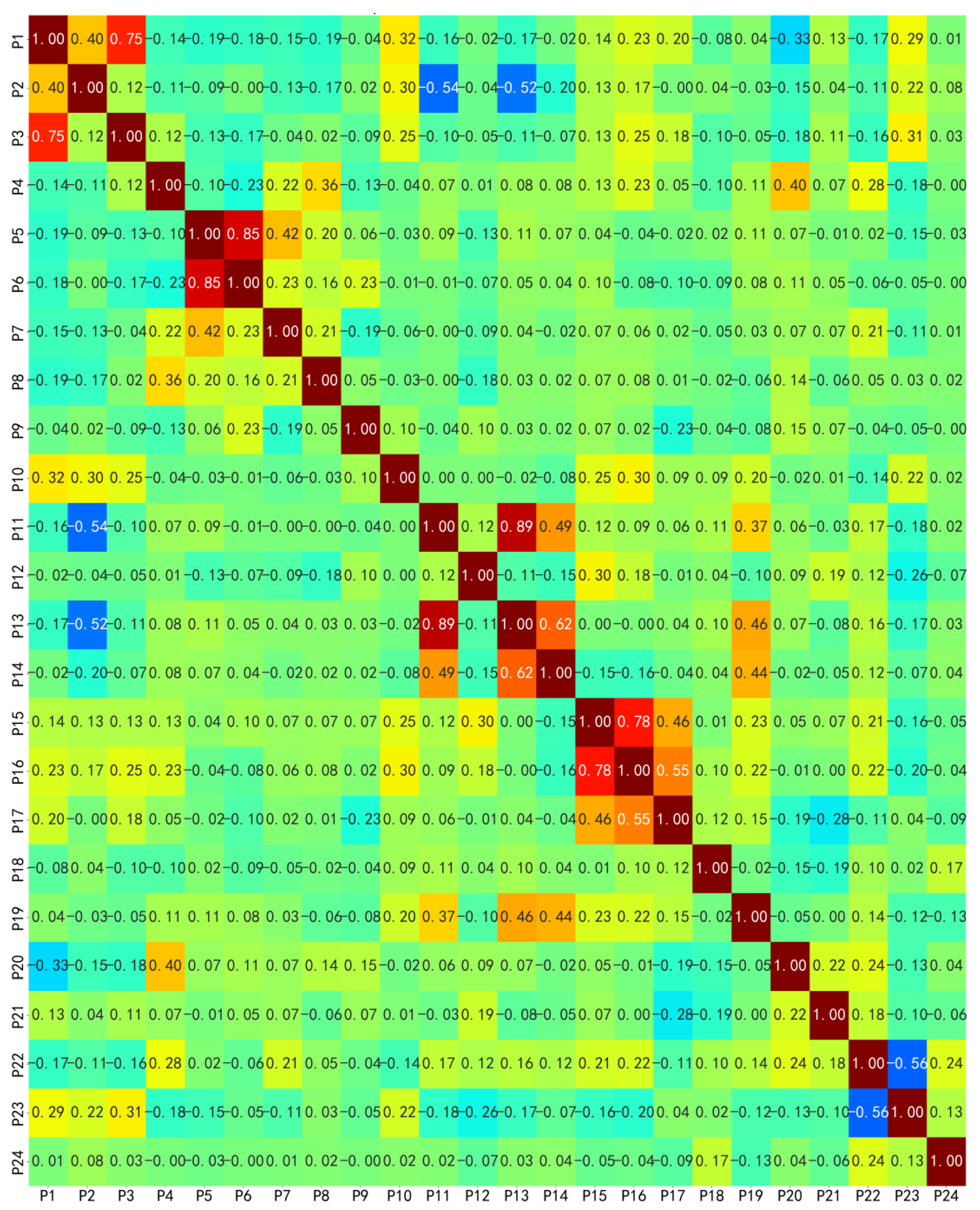
Spearman correlation coefficient is a non parametric statistic used to measure the degree of correlation between two variable rankings. It evaluates monotonic relationships by comparing the rank of variables, whether linear or nonlinear. Its value range is [−1, 1], where 1 represents complete positive correlation, −1 represents complete negative correlation, and 0 represents no correlation. Figure 4 shows the distribution of Spearman correlation coefficients between various influencing parameters and the degree of significance. According to correlation theory, it is generally believed that correlation coefficients between 0 and 0.3 indicate no correlation or very weak correlation, 0.3 to 0.6 indicate weak correlation, 0.6 to 0.7 indicate moderate correlation, and 0.7 to 1 indicate strong correlation. Through quantitative analysis of Spearman correlation, it was found that the correlation coefficients between injected fluid volume and sand volume, operating pressure and breakdown pressure, cumulative fluid production before measures and production months, and other two characteristic parameters were all greater than 0.7 (as shown in Table 2). It was ultimately determined to delete the characteristic parameters of injected fluid volume, operating pressure, and production months, leaving a total of 20 characteristic parameters including reservoir thickness, vertical thickness, resistivity, neutron, porosity, permeability, oil saturation, clay content, acid amount, sand amount, sand ratio, pumping rate, breakdown pressure, pumping-stop pressure, fracturing types, flowback volume, initial daily liquid production, daily liquid production before stimulation, cumulative liquid production before stimulation, production days, and increase in oil production.

Figure 4. Spearman correlation matrix of feature parameters.

Table 2. Feature parameter correlation filtering table.

Feature A	Correlation	Feature B	Deleted Feature Parameters
Porosity	0.7	Acoustic interval	Acoustic interval
Acid amount	0.8	Sand amount	Acid amount
Working pressure	0.8	Breakdown pressure	Working pressure
Cumulative liquid production before stimulation	0.7	Production days	Production days

3. Analysis of the Main Control Factors

3.1. Introduction to Basic Method Principles

To avoid relying on a single evaluation method and obtain more reliable results, we employ a combination of the Pearson correlation coefficient, Random Forest, and recursive feature elimination algorithm. This approach aims to identify the primary geological and engineering factors that influence the fracturing effect of different types of oil wells.

The Pearson correlation coefficient is a statistical measure used to assess the degree of linear association between two continuous variables.

$$\begin{array}{c}\mathit{r}={\displaystyle \frac{{\sum }_{\mathit{i}=1}^{\mathit{n}} \left({\mathit{X}}_{\mathrm{i}}-\stackrel{\mathrm{-}}{\mathit{X}}\right)\left({\mathit{Y}}_{\mathit{i}}-\stackrel{\mathrm{-}}{\mathit{Y}}\right)}{\sqrt{{\sum }_{\mathit{i}=1}^{\mathit{n}} ({\mathit{X}}_{\mathit{i}}-\stackrel{\mathrm{-}}{\mathit{X}}{)}^2}\sqrt{{\sum }_{\mathit{i}=1}^{\mathit{n}} ({\mathit{Y}}_{\mathit{i}}-\stackrel{\mathrm{-}}{\mathit{Y}}{)}^2}}}\end{array}$$

(3)

In the formula, $\mathit{r}$ represents the correlation coefficient, ${\mathit{X}}_{\mathit{i}}$, ${\mathit{Y}}_{\mathit{i}}$ represents the i-th sample of the feature parameter, $\stackrel{\mathrm{-}}{\mathit{X}}$, $\stackrel{\mathrm{-}}{\mathit{Y}}$ represents the mean value of the feature parameter, and $\mathit{n}$ is the number of samples.

Recursive Feature Elimination (RFE) is a greedy optimization algorithm that iteratively constructs models to identify the most effective feature subset. The process begins with an initial feature set comprising 20 selected parameters. Using machine learning, RFE calculates an importance score for each feature and employs cross-validation to assess the set’s classification accuracy. Based on feature performance, the weakest features are then removed. The remaining features form a new subset used to rebuild the model. This cycle—recalculating feature importance, evaluating accuracy via cross-validation, and eliminating the least important features—iterates until all features are processed. Throughout RFE, the elimination sequence directly reflects feature importance, with features removed earlier deemed less significant. The inherent mechanism of Random Forest (RF) lies primarily in its dual characteristics of randomness and integration. Randomness, achieved through random sampling of data points and random selection of features, ensures each decision tree is unique, thereby enhancing model diversity. Integration, manifested in combining the predictions of multiple decision trees via majority vote or averaging, effectively reduces model variance and consequently improves stability and accuracy. For a given test sample, each of the N independently constructed decision trees casts a classification vote. The final output of the algorithm is determined by the class receiving the majority of votes.

3.2. Analysis of Evaluation Results Using a Single Method

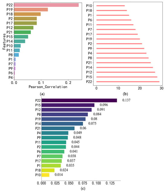
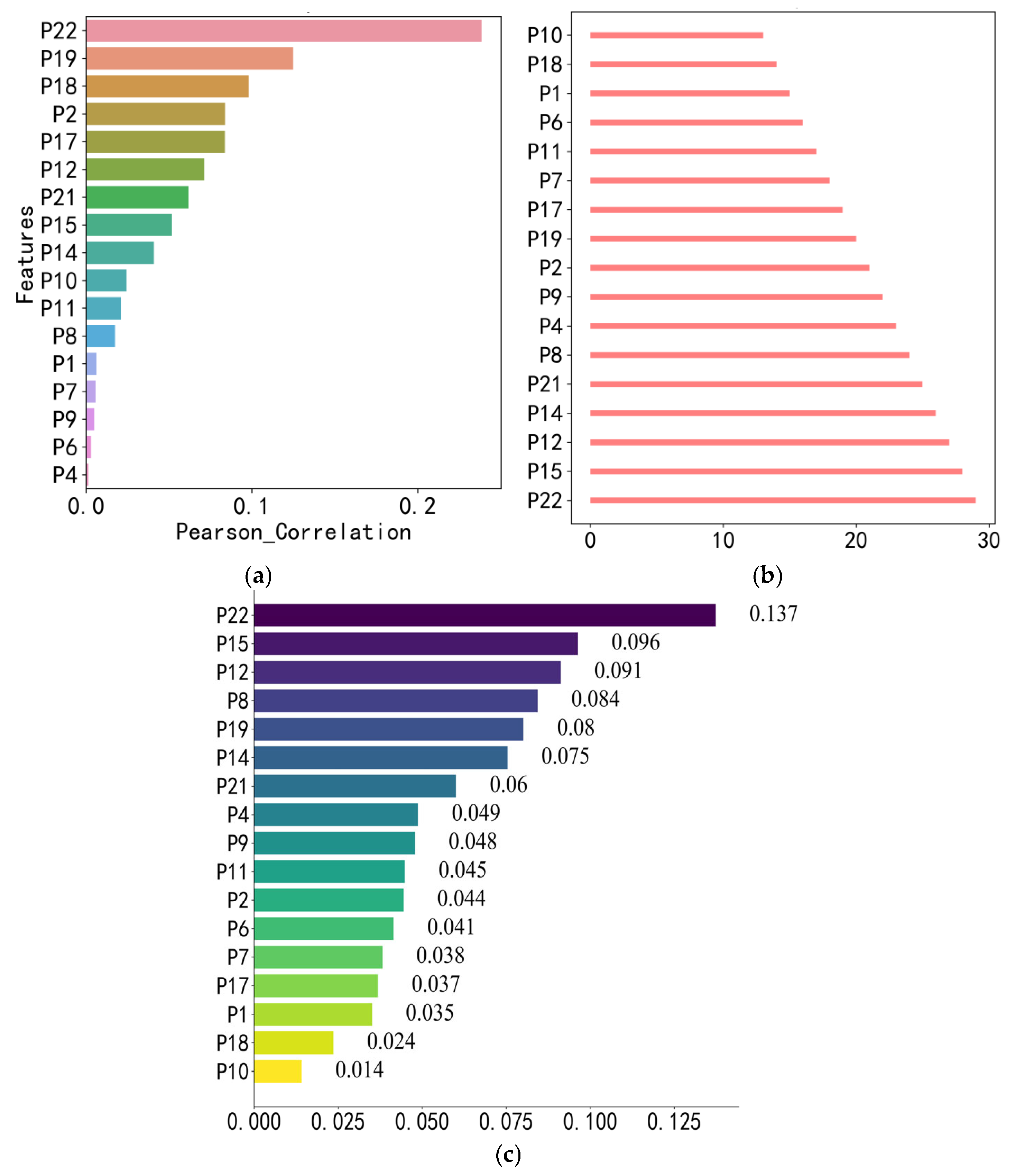
Based on the three individual evaluation methods introduced earlier for identifying key factors controlling production capacity, using different stages of production capacity as evaluation metrics, the resulting importance rankings derived from the same method show minor variations. Figure 5 presents the parameter importance results using effective-period incremental oil production as the evaluation metric.

Figure 5. Evaluation results of single method. (a) Pearson correlation coefficient method; (b) Recursive Elimination Method; (c) Random Forest Algorithm.

According to the Pearson correlation coefficients (Figure 5a), the top 8 factors, ranked by the absolute value of their coefficients, are: Net pay thickness; Sand ratio (proppant concentration); Pumping-stop pressure; Fracturing fluid type; Flowback volume; Initial daily liquid production; Pre-stimulation daily liquid production; Pre-stimulation cumulative liquid production.

The Recursive Feature Elimination (RFE) method results (Figure 5b) identify the following key factors: Oil saturation; Sand ratio (proppant concentration); Pumping rate; Breakdown pressure; Flowback volume; Initial daily liquid production; Pre-stimulation daily liquid production; Pre-stimulation cumulative liquid production.

The Random Forest (RF) method results (Figure 5c) indicate that the ranking of influential factors for dynamic production capacity metrics remains somewhat variable. Factors with greater impact include the following: Acid volume; Proppant volume; Pumping rate; Breakdown pressure; Flowback volume; Initial daily liquid production; Pre-stimulation cumulative liquid production.

3.3. Analysis of Comprehensive Evaluation Results of Main Control Factors

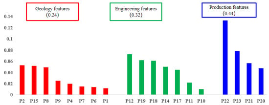
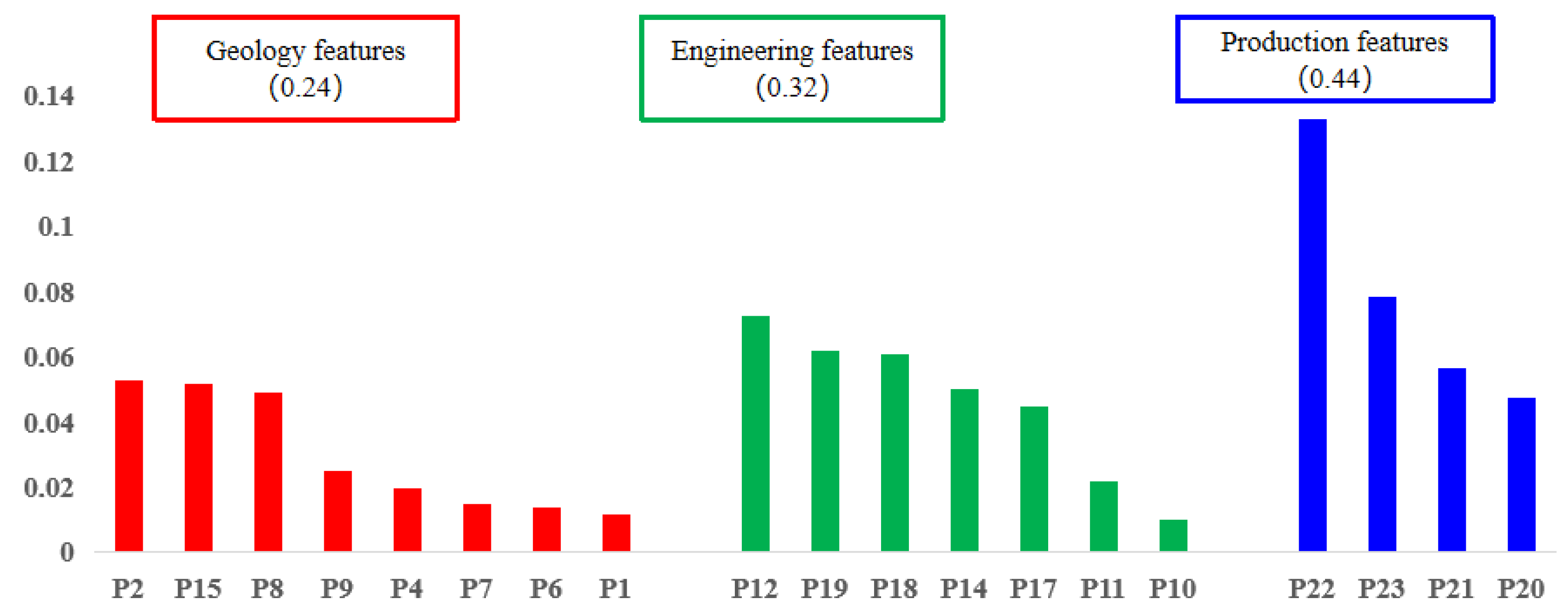
We analyzed the main control factors affecting production capacity using the Pearson correlation coefficient, recursive feature elimination (RFE), and Random Forest algorithms. However, due to the distinct characteristics (advantages, disadvantages, and analytical focus) of each method, the identified key factors differed slightly. The importance scores from the Pearson correlation, Random Forest, and RFE analyses were normalized to a uniform scale, and a weighted average was applied to determine the composite importance score for each factor.

Figure 6 ranks the importance of geological and engineering parameters. Post-fracturing incremental oil production serves as the evaluation index for productivity. The importance scores are 0.24 for geological parameters, 0.32 for engineering parameters, and 0.44 for production parameters. Based on the weighted evaluation from the three methods, production parameters emerge as the primary controlling factors affecting post-fracturing oil increase. Key parameters include Geological parameters (Vertical thickness, fracture pressure, and oil saturation), engineering parameters (sand ratio, fluid injection volume, and fracturing method), production parameters (pre-fracturing cumulative fluid production, production months, pre-fracturing cumulative oil production, and the post-fracturing incremental oil production itself).

Figure 6. Ranking of the importance of geological and completion parameters.

3.4. Global Explanation of Model Based on SHAP

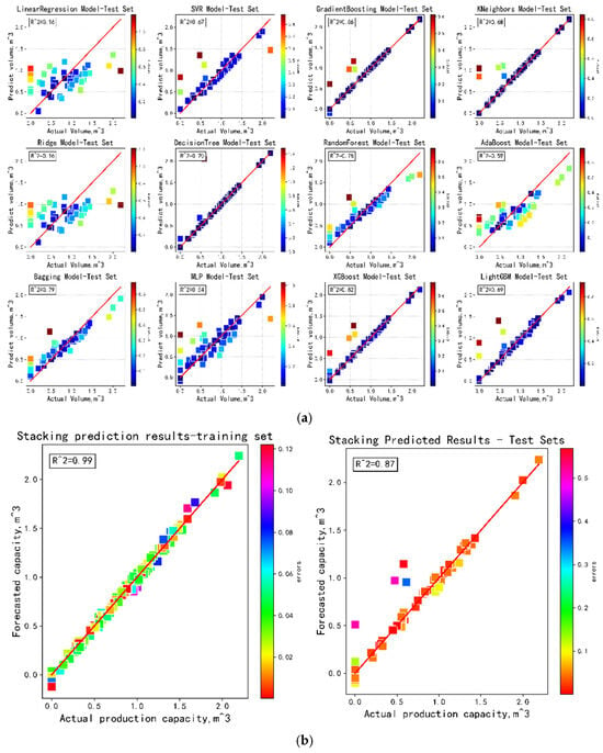
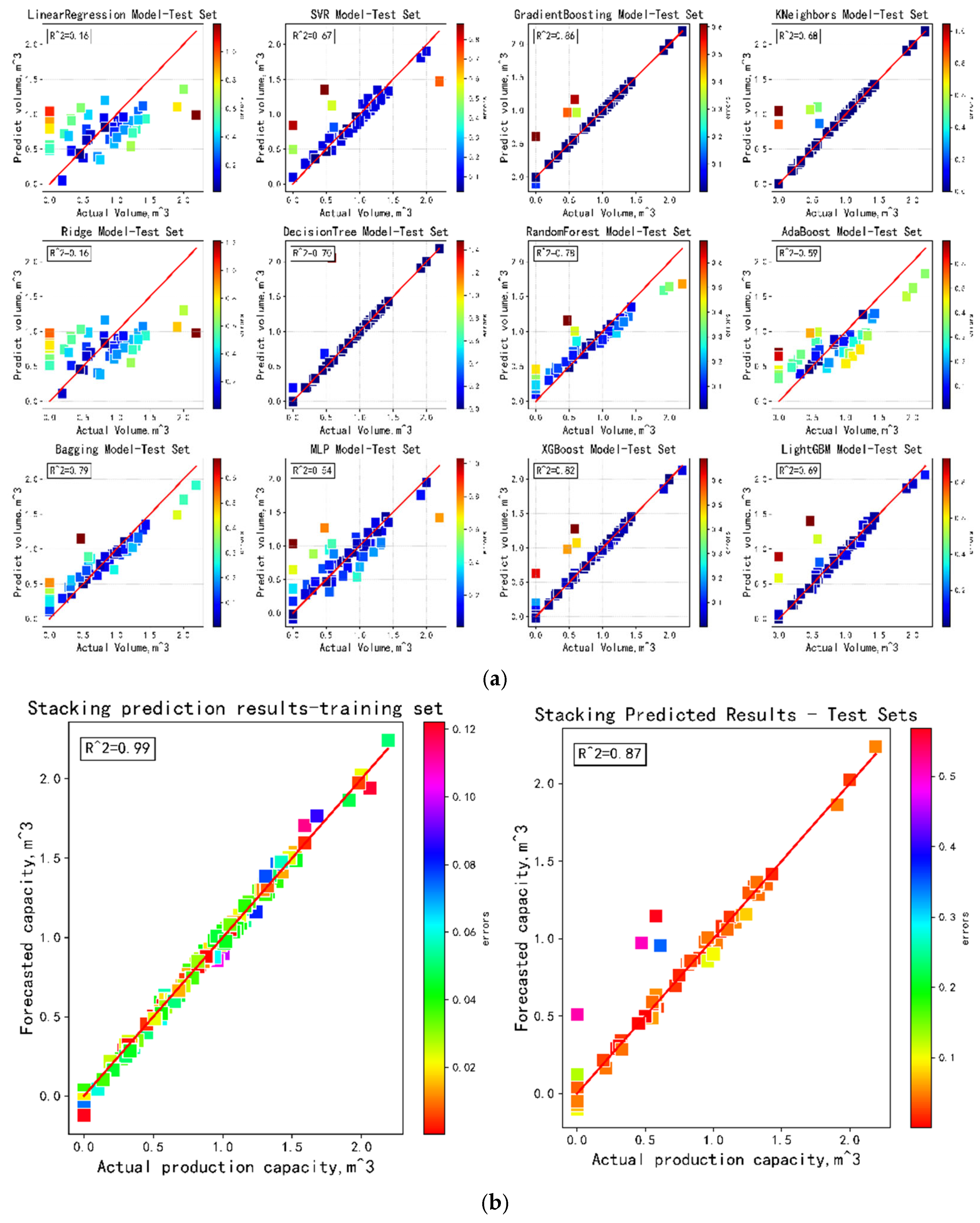
Stacking is an ensemble algorithm that integrates multiple machine learning models hierarchically. Stacking’s key advantage lies in using multi-perspective predictions from diverse base models as meta-features, combining their strengths to typically outperform individual models. As shown in Figure 7, in our experiments, base models included Random Forest (R² = 0.78), Gradient Boosting (0.80), LightGBM (0.79), AdaBoost (0.60), Decision Tree (0.70), and Support Vector Machine (0.67). Stacking integration significantly improved accuracy, achieving a test set R² of 0.87 for the production capacity prediction model. SHAP (SHapley Additive exPlanations), based on cooperative game theory’s Shapley value, interprets machine learning predictions. The Shapley value quantifies each feature’s fair contribution to the model outcome. We applied SHAP analysis to our capacity prediction model, transforming multi-scale, interdependent features into comparable normalized values. This enhances model interpretability, enables quantitative assessment of individual feature impacts, increases model credibility, and resolves the “black box” limitation of conventional machine learning.

Figure 7. Relationship between real value and predicted value of Stacking model. (a) Meta model; (b) stacking model.

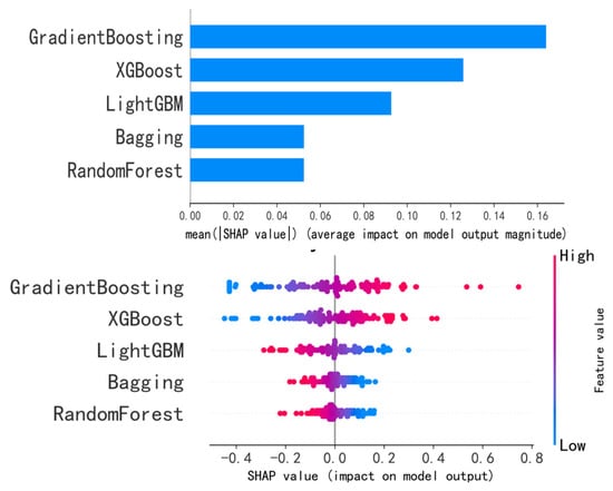
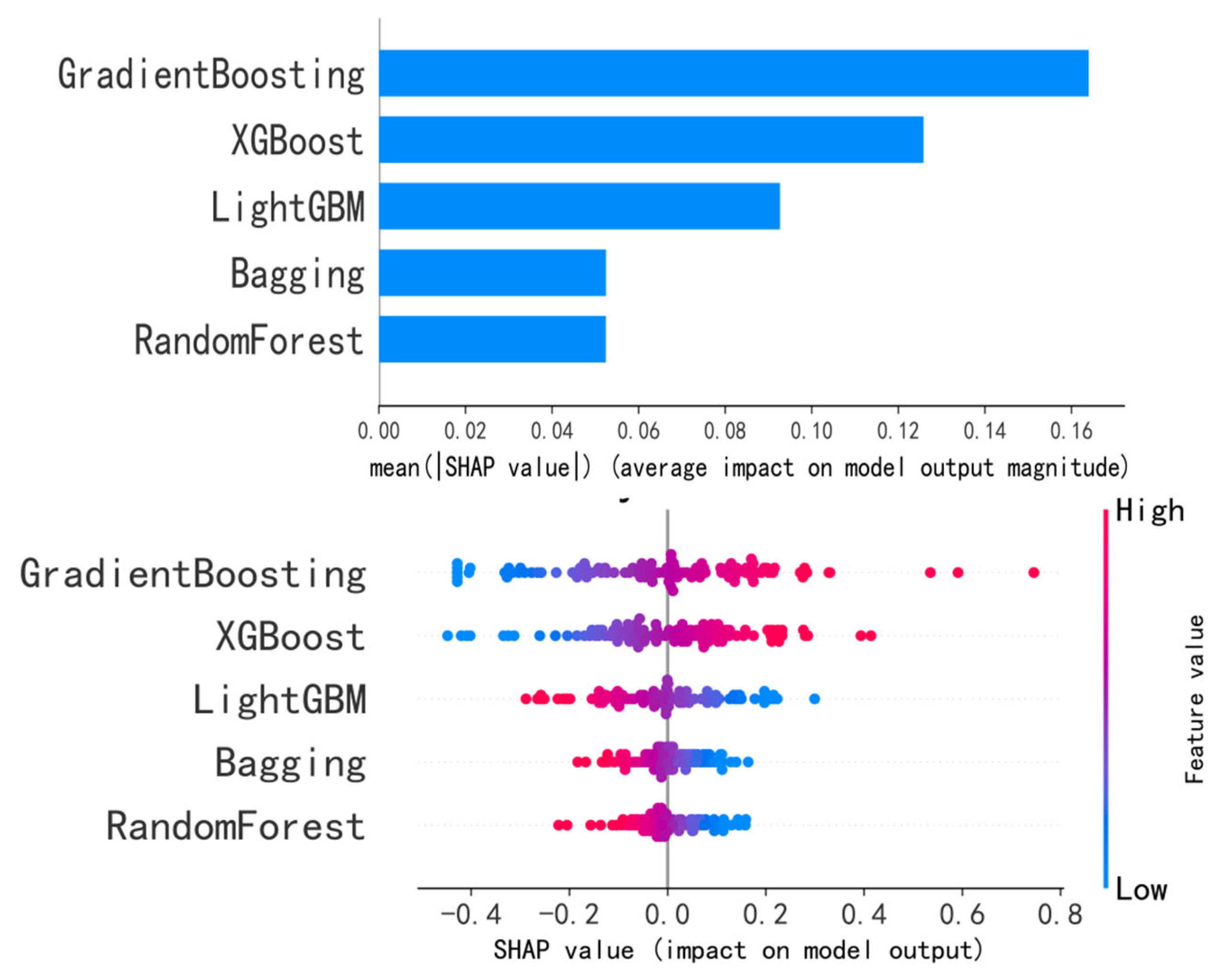
As shown in Figure 8, SHAP-based interpretation of the Stacking model reveals that the Bagging and XGBoost base learners exert the strongest influence. Among the feature parameters, production parameters—notably cumulative fluid production prior to measures and production months—remain dominant, reinforcing the earlier main controlling factor analysis.

Figure 8. SHAP summary of Meta model.

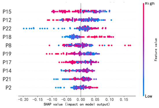
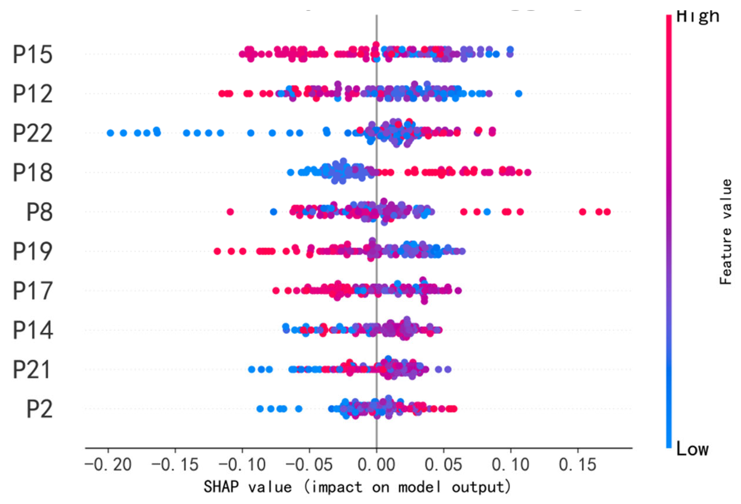
Figure 9 illustrates the distribution of SHAP values for geological and engineering parameters influencing the incremental oil production index during the effective period. Each point corresponds to a fractured well, with features ranked vertically by descending importance. The horizontal axis represents the SHAP value output by the model. Point color indicates feature magnitude: red denotes higher values, while blue denotes lower values. A positive SHAP value signifies a positive impact on incremental oil production, whereas a negative value indicates a detrimental effect. As shown in Figure 9, the following parameters exhibit a positive correlation with predicted daily incremental oil production: Pre-fracturing cumulative fluid production, Production months, Initial daily oil production, Vertical thickness. These factors collectively increase predicted production. Conversely, pre-fracturing water cut, pre-fracturing daily oil production, and initial water cut demonstrate complex, nonlinear relationships with the predicted increment. Notably, selecting volumetric fracturing as the stimulation method shows the highest feature dependence and contributes positively to increased oil production.

Figure 9. Visualization of SHAP values for the overall sample.

4. Prediction Method for Time Series Production Data

4.1. Similarity Analysis

①

Euclidean distance

The Euclidean distance is used to measure the linear distance between two sample points. It is the distance between sample points in Euclidean space, usually expressed as the following formula:

$${\mathit{d}}_{\mathrm{Euclidean}}\left({\mathit{x}}_{\mathit{i}},{\mathit{x}}_{\mathit{j}}\right) = \sqrt{{\left({\mathit{x}}_{\mathit{i}1}-{\mathit{x}}_{\mathit{j}1}\right)}^2+{\left({\mathit{x}}_{\mathit{i}2}-{\mathit{x}}_{\mathit{j}2}\right)}^2+\cdots +{\left({\mathit{x}}_{\mathit{in}}-{\mathrm{x}}_{\mathit{jn}}\right)}^2}$$

(4)

where x_i and x_j are two sample points, x_i1, x_i2, …, x_in are the feature values of sample point x_i, and x_j1, x_j2, …, x_jn are the feature values of sample point x_j. Euclidean distance is a simple distance calculation method that is easy to understand, computationally efficient, and highly effective in reflecting the similarity relationship between two sequences. It is a commonly preferred similarity measurement method. However, it requires that the two sequences being compared have the same length, which limits its flexibility and ability to bend and stretch along the time axis. Therefore, it is difficult to capture the deformation characteristics of time series, and it is necessary to combine it with dynamic time warping distance methods.

②

Dynamic time warping distance

Dynamic Time Warping (DTW) is an algorithm used to measure the similarity between two time series, especially for sequence alignment with different lengths or inconsistent local speeds. Its core idea is to find the optimal path between two sequences by aligning the time axes nonlinearly, so that the cumulative distance on the path is minimized, thus achieving similarity measurement for different time series. Given two time series $\mathit{P} = ({\mathit{p}}_1,{\mathit{p}}_2,\cdots ,{\mathit{p}}_{\mathit{m}})$ and $\mathit{Q} = ({\mathit{q}}_1,{\mathit{q}}_2,\cdots ,{\mathit{q}}_{\mathit{n}})$, with lengths m and n (m ≥ n), the dynamic time warping distance between the two sequences can be expressed as

$$\mathit{D}\left(\mathit{P},\mathit{Q}\right)=\underset{\mathit{p}}{ \min }\sum _{\mathrm{k}=1}^{\mathrm{m}}\mathrm{d}\left({\mathrm{p}}_{\mathrm{k}}\right)$$

(5)

where d(p_k) is the distance between point p_k and some point q. Compared with traditional lockstep metrics such as Euclidean distance, it can better handle time lags, advances, or deformations in time series, and has certain robustness to noise and local fluctuations in time series. However, when the length of the time series is large, the computational burden increases significantly.

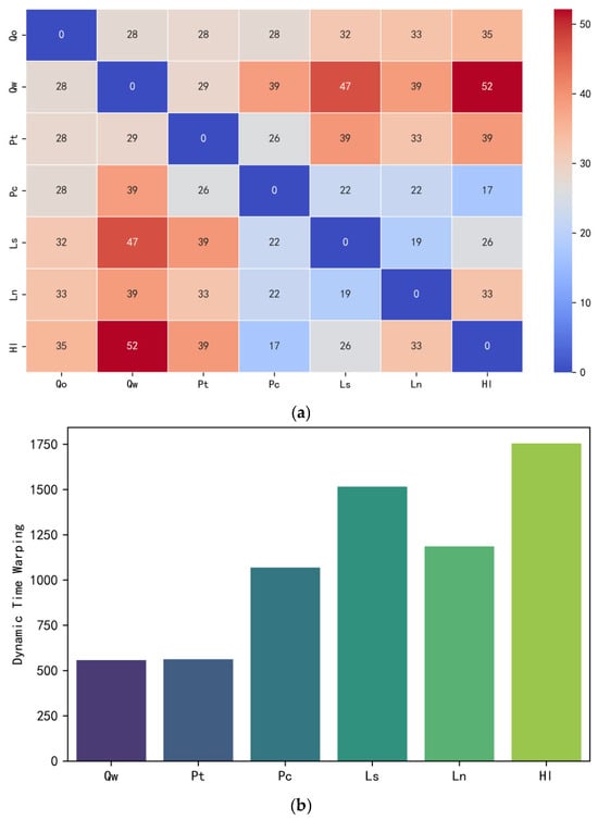
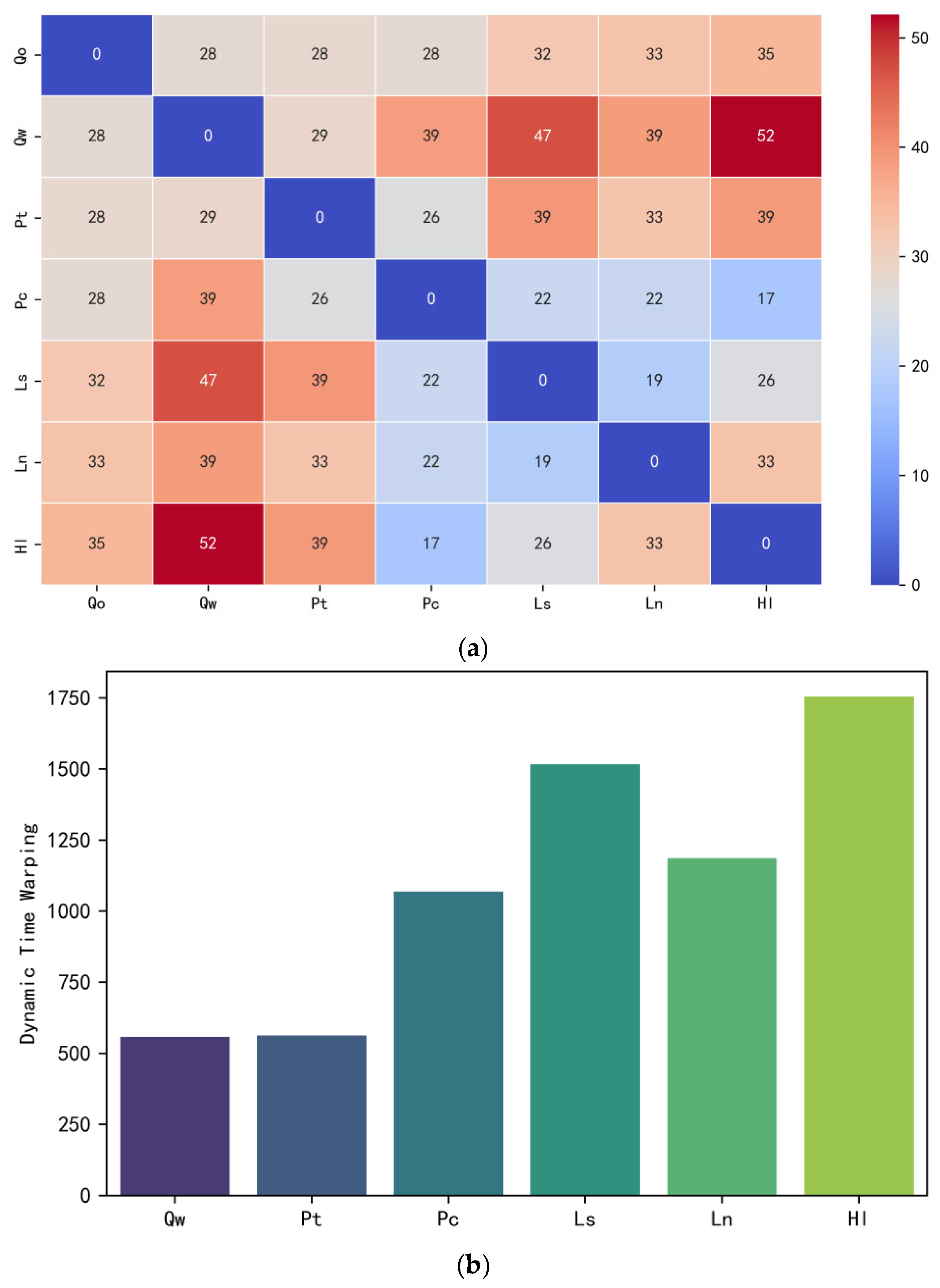
The dynamic production dataset of a well in the Changqing Bai 153 well area underwent preprocessing, which mainly involved outlier detection, missing value handling, and data normalization. Subsequently, the target sequence and comparison sequence were determined. The target sequence was daily oil production, while the comparison sequence included daily water production, oil pressure, casing pressure, stroke, stroke rate, and dynamic fluid level.

Based on the ED and DTW algorithms, a study on the time series similarity of Well Bai 154 was conducted through Figure 10. Through comparison, it was found that the parameters that affect the production sequence are: Euclidean distance, water production rate > casing pressure > oil pressure > stroke > stroke rate > dynamic fluid level. DTW distance: water production rate > oil pressure > casing pressure > stroke rate > stroke > dynamic fluid level. Based on the DTW distance results, the four characteristic parameters of water production rate, oil pressure, casing pressure, and stroke rate were used as constraints for subsequent prediction models.

Figure 10. Visualization of similarity analysis. (a) Euclidean Distance Heatmap; (b) DTW.

4.2. Prediction Method Based on Physical Constraint Attention Mechanism

①

Gated Recurrent Unit (GRU)

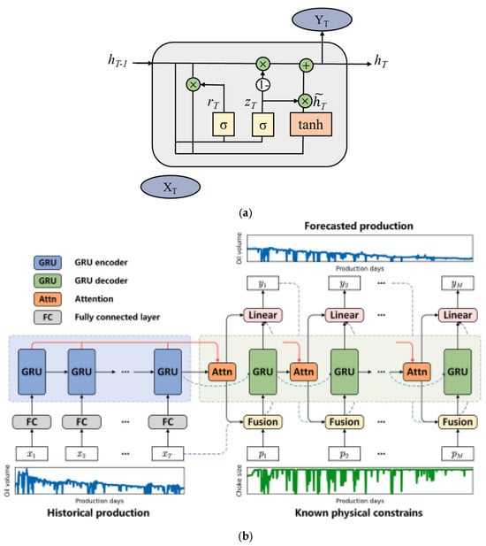
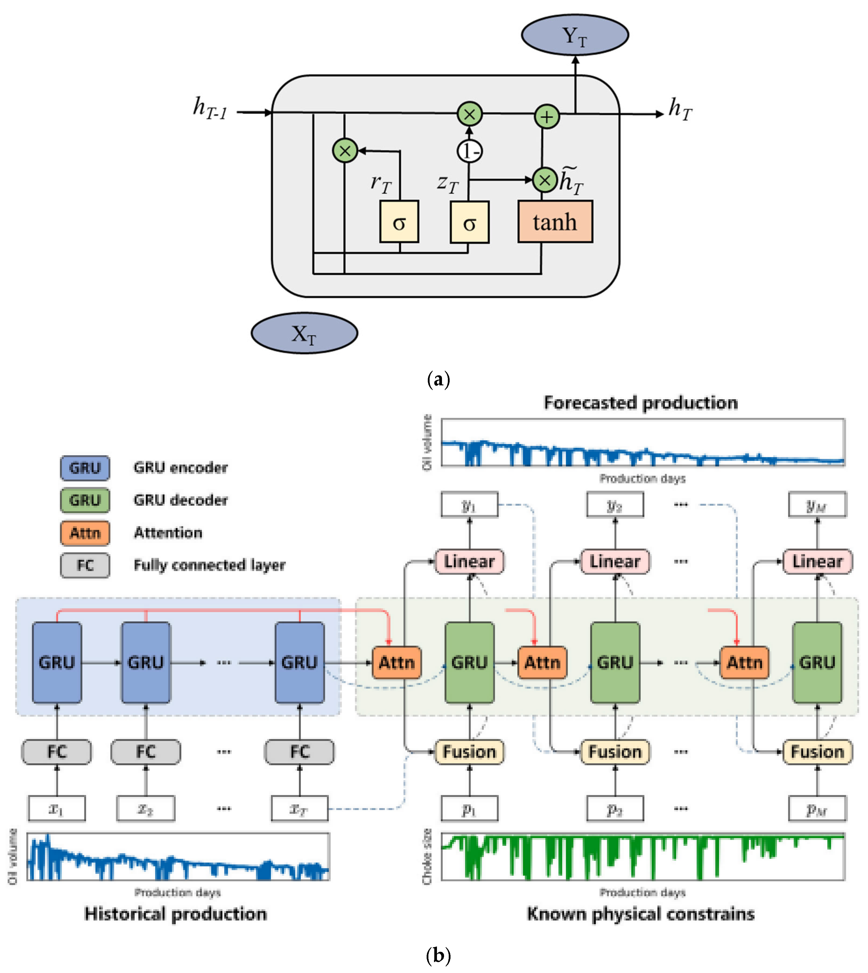
GRU (Gated Recurrent Unit) is a variant of RNN (Recurrent Neural Network) that employs a gated structure to address the long-term dependency problem. Compared to LSTM (Long Short-Term Memory), GRU features a simpler architecture while achieving comparable prediction performance. The core GRU consists of two gates: a reset gate and an update gate. The update gate (z_t), expressed as

$${\mathit{r}}_{\mathit{T}}=\mathit{\sigma }({\mathit{W}}_{\mathit{r}}\cdot [{\mathit{h}}_{\mathit{T}-1},{\mathit{X}}_{\mathit{T}}]+{\mathit{b}}_{\mathit{r}})$$

(6)

where Wr and br are the weight matrix and bias matrix of the update gate, respectively.

The reset gate (z_t) governs the degree of past information forgotten, constrained to values within [0, 1]. Specifically, lower values (closer to 0) result in more extensive forgetting. The gate’s mathematical form is

$${\mathit{z}}_{\mathit{T}}=\mathit{\sigma }({\mathit{W}}_{\mathit{z}}\cdot [{\mathit{h}}_{\mathit{T}-1},{\mathit{X}}_{\mathit{T}}]+{ \mathit{b}}_{\mathit{z}})$$

(7)

where W_z and b_z are the weight matrix and bias matrix of the reset gate, respectively.

Following processing through the update and reset gates, the input yields the candidate hidden state at T as

$${\stackrel{\mathrm{~}}{\mathit{h}}}_{\mathit{T}}=\mathit{tanh}({\mathit{W}}_{\mathit{h}}\cdot [{\mathit{h}}_{\mathit{T}-1}\odot {\mathit{r}}_{\mathit{T}},{\mathit{X}}_{\mathit{T}}]+{\mathit{b}}_{\mathit{h}})$$

(8)

where W_h and b_h are the weight matrix and bias matrix of the unit hidden state, respectively, and $\odot$ is the Hadamard product. Finally, we obtain the output h_T at time step T:

$${\mathit{h}}_{\mathit{T}} = (1 -{ \mathit{z}}_{\mathit{T}})\odot {\mathit{h}}_{\mathit{T}-1} + {\mathit{z}}_{\mathit{T}}\odot {\stackrel{\mathrm{~}}{\mathit{h}}}_{\mathit{T}}$$

(9)

②

Attention Mechanism (AT)

The attention mechanism computes normalized weights representing input element relevance. This involves scoring query-key pairs through a similarity function.

$${\mathit{e}}_{\mathit{t}}=\mathit{tanh}({\mathit{W}}_{\mathit{t}}{\mathit{h}}_{\mathit{t}}+{\mathit{b}}_{\mathit{h}})$$

(10)

Normalization: Use the softmax function to normalize the scores and obtain the weight corresponding to each key.

$${\mathit{\alpha }}_{\mathit{t}}={\displaystyle \frac{\mathit{exp}\left({\mathit{e}}_{\mathit{t}}\right)}{{\sum }_{\mathit{t}=1}^{\mathit{T}}\mathit{exp}\left({\mathit{e}}_{\mathit{t}}\right)}}$$

(11)

Weighted sum: The final attention output is obtained by weighted sum of the corresponding values (Value) according to the weights.

$$\mathit{c}=\sum _{\mathit{t}=1}^{\mathit{T}}{\mathit{\alpha }}_{\mathit{t}}{\mathit{h}}_{\mathit{t}}$$

(12)

The architecture, modified from the deep-learning model [26], is depicted in Figure 11. A GRU encoder module encodes the historical production input sequence. Recognizing that production depends on reservoir geological conditions and human-adjusted development plans, known control parameters (e.g., oil pressure, nozzle size) are injected as external constraints into the feature extraction module. (When sufficient data exists, seismic logging data can also be incorporated as a constraint via convolutional neural network processing.) The encoded sequence (input), hidden state, and physical constraint sequence are concatenated and fed into the GRU decoder module. The decoder’s output undergoes linear transformation to generate production predictions. During training, either the true value or the predicted value for the next timestep is strategically selected as the subsequent input. This mitigates cumulative error propagation, accelerates convergence, and enhances prediction performance.

Figure 11. Model framework diagram [26]. (a) GRU neural network unit structure diagram.

③

Data preprocessing

Here we adopt a multi-input and multi-output prediction strategy, thus the data split also needs to follow this principle. Due to the adoption of a multi input multi output prediction strategy, the construction method of multi-step temporal prediction samples needs to be adjusted accordingly. For a raw yield data of size (N, 3), the window size is set to w and the prediction step size H is set to 3, which means predicting the yield for the next 3 days based on the past w days’ yield and exogenous variable data. Firstly, take the data from day 1 to day w as the input for the first sample, and the output from day w + 1 to w + 3 as the output for the first sample. Construct the first input-output pair for the sample. Subsequently, slide the sliding window down for 1 day, taking the data from day 2 to day w + 1 as the input for the second sample, and the output from day w + 2 to day w + 5 as the output for the second sample. Construct the second input-output pair sample, and slide the sliding window down again for 1 day. Repeat the above process until the production data on the Nth day is included in the output. Thus, a multi-step input-output pair with an input size of (N − w − H + 1, w, 3) and an output dimension of (N − w − H + 1, 3) is constructed using a sliding window, with a total sample size of n = N − w − H + 1.

In the k-fold cross-validation method, the dataset is divided into k subsets. A unique subset is selected as the test set, while the remaining k − 1 subsets are used as the training set. This process is repeated k times, and the final model error is determined by calculating the average prediction error across all k test sets. This method ensures that all samples in the training set have the opportunity to participate in both training and testing, providing a more fair evaluation of the model’s robustness and generalization ability.

First, fill in the null values with zeros, and then perform z-score normalization on the data of each wellbore to eliminate the influence of dimensions. The formula is

$$\stackrel{\mathrm{~}}{\mathit{x} }={\displaystyle \frac{\mathit{x}-\overline{\mathit{x}}}{\mathit{\sigma }}}$$

(13)

where x represents a feature, $\overline{x}$, $\sigma$ represent the mean and variance of the feature in the training set, respectively, and $\tilde{x}$ represents the scaled feature.

This article sets three evaluation indicators: mean absolute error (MAE), mean squared error (MSE), and absolute coefficient (R²), with the specific calculation formulas shown in Equations (14)–(16):

$$\mathit{MAE} = {\displaystyle \frac{1}{\mathit{N}}}\sum _{\mathit{i} = 1}^{\mathit{N}}/{\mathit{y}}_{\mathit{i}} - \mathit{f}({\mathit{x}}_{\mathit{i}})/$$

(14)

$$\mathit{MSE}={\displaystyle \frac{{\sum }_{\mathit{i}=1}^{\mathit{N}}\left({\mathit{y}}_{\mathit{i} }\text{-} \mathit{f}\right({\mathit{x}}_{\mathit{i}}){)}^2}{\mathit{N}}}$$

(15)

$${\mathit{R}}^2=1-{\displaystyle \frac{{\sum }_{\mathit{i}=1}^{\mathit{N}}({\mathit{y}}_{\mathit{i}}-\mathit{f}({\mathit{x}}_{\mathit{i}}){)}^2}{{\sum }_{\mathit{i}=1}^{\mathit{N}}({\mathit{y}}_{\mathit{i}}-\overline{\mathit{y}}{)}^2}}$$

(16)

where N is the number of samples, ${\mathit{y}}_{\mathit{i}}$ is the true value of the target variable for the ith sample, $\mathit{f}\left({\mathit{x}}_{\mathit{i}}\right)$ represents the predicted value of the model with input x_i, and $\overline{\mathit{y}}$ is the mean of the target variables for all samples.

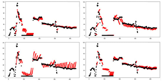
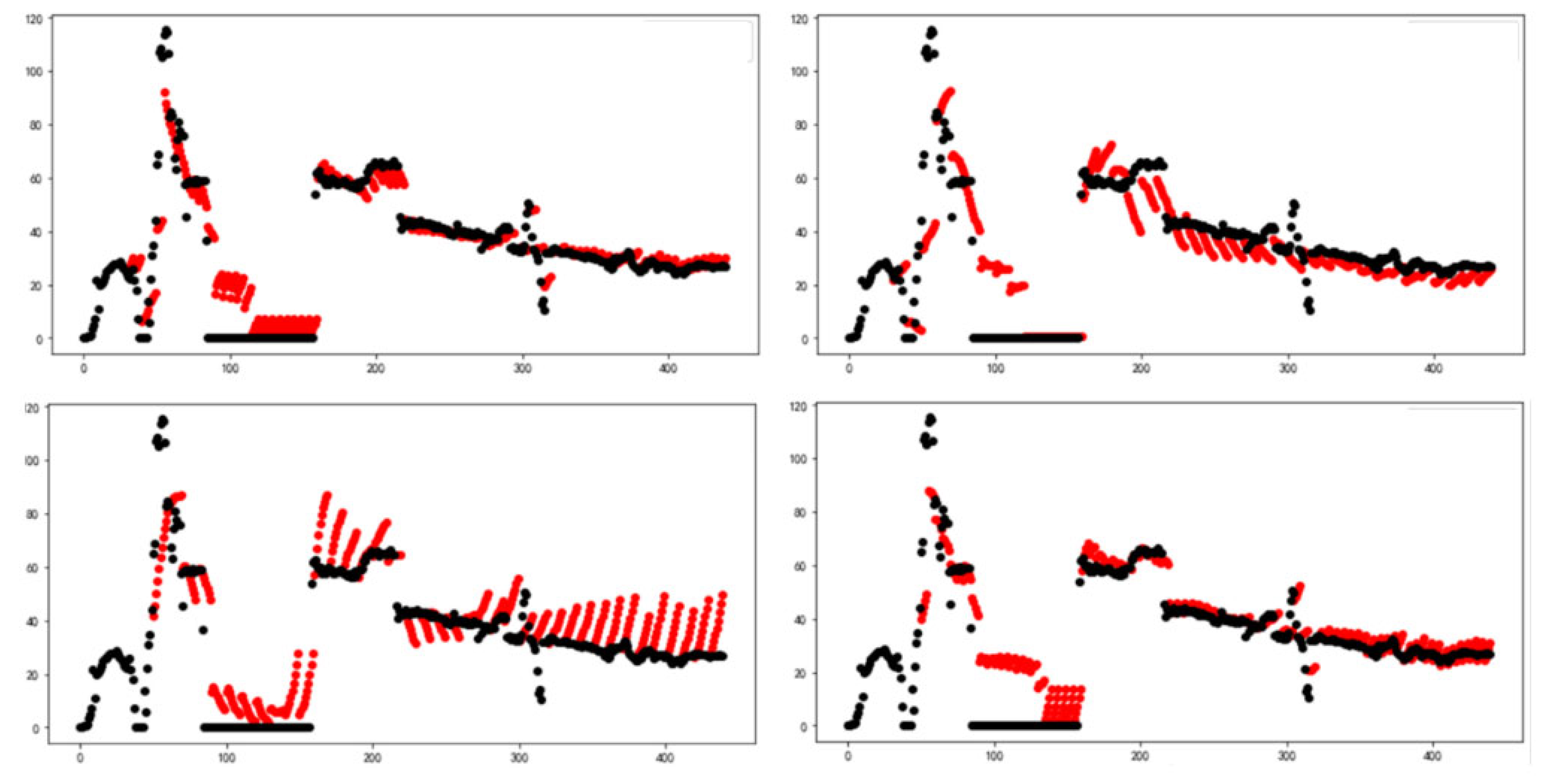
First, we conduct the hype-parameter optimization. The Combinations of model hyperparameters is shown in Table 3. Four schemes (as shown in Table 4) were proposed, with oil production as the target, to predict the performance of four wells (well-A to well-D) without adding physical constraints. The comparison of absolute coefficient means showed that parameter combination 1 had the highest accuracy and relatively good prediction performance. The prediction effect without physics constraint is shown in Figure 12.

Table 3. Combinations of model hyperparameters.

History Window Size	Prediction Window Size	Number of GRU Layers	Number of Neurons	R2
30	5	2	80	0.81449
30	10	3	100	0.7042525
50	10	2	100	0.7350375
50	5	3	80	0.794865

Table 4. Combination of physical constraint parameters.

	Target	Constraint
1	Oil rate	/
2	Oil rate	oil pressure
3	Oil rate	oil pressure, casing pressure, stroke rate
4	Oil rate	water production rate, oil pressure, casing pressure, and stroke rate

Figure 12. Comparison of prediction effects of production wells.

The model takes oil production as the prediction target and compares the prediction effects of different combinations of constraint parameters to explore the optimal combination of constraint parameters to achieve better prediction accuracy. The combinations are shown in Table 4.

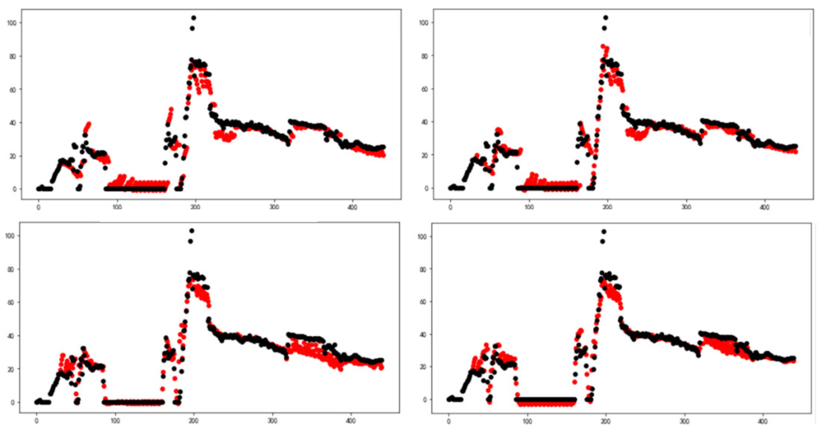
The constraint sequences of the four combinations were inputted into the model separately, and the prediction accuracy is shown in Table 5. As the inputted yield-related parameters increased, the average absolute error and mean square error of the four wells showed a downward trend, and the absolute coefficient increased, indicating better and better prediction results. Among them, the constraint parameter combination 5 had the highest prediction accuracy, and the prediction effect is shown in Figure 13. The mean values of MSE, MAE, and R² were 0.09929, 0.18686, and 0.90454, respectively, which was 9% higher than that of combination 1.

Table 5. Prediction accuracy of different constraint combinations.

	MSE					MAE					R2
	Well-A	Well-B	Well-C	Well-D	Mean	Well-A	Well-B	Well-C	Well-D	Mean	Well-A	Well-B	Well-C	Well-D	Mean
1	0.16761	0.12716	0.2393	0.22156	0.188908	0.20502	0.21843	0.26357	0.25251	0.234883	0.83584	0.86975	0.76501	0.78736	0.81449
2	0.17501	0.09826	0.23352	0.20286	0.177413	0.25209	0.19101	0.27851	0.23652	0.239533	0.82904	0.89939	0.77067	0.80563	0.826183
3	0.11771	0.0867	0.14671	0.16466	0.128945	0.20185	0.17802	0.21727	0.21292	0.202515	0.88388	0.91109	0.85616	0.84215	0.87332
4	0.07855	0.07949	0.09374	0.14538	0.09929	0.17073	0.14746	0.18253	0.24672	0.18686	0.92185	0.92779	0.9081	0.86042	0.90454

Figure 13. Prediction effect of discontinuous production wells in constraint combination 4.

5. Conclusions

The productivity of fractured wells is influenced by numerous complex factors with significant data noise. A single machine learning algorithm struggles to effectively capture the relationships between feature parameters and their dynamic impact on productivity indicators. After preprocessing the raw data, this study employs the Spearman correlation coefficient to eliminate redundant features. It then integrates recursive feature elimination (RFE) and Random Forest algorithms to evaluate the main controlling factors for productivity indicators. The analysis clearly identifies production parameters as the primary controls affecting post-fracturing oil increment. Production Parameters: Pre-fracturing cumulative fluid production, production months, pre-fracturing cumulative oil production, and post-fracturing oil increment. Based on Dynamic Time Warping (DTW) distance results, four characteristic parameters—water production rate, oil pressure, casing pressure, and stroke rate—were selected as constraints for subsequent prediction models. The model incorporates an attention mechanism and forced next input selection. Without physical constraints, prediction accuracy for discontinuous production wells reached 81.45%. Performance improved significantly as constraint combinations were incrementally applied, achieving 90.45% accuracy.

References

- Zhu, W.; Yue, M.; Liu, Y.; Liu, K.; Song, Z. Research progress on tight oil exploration in China. Chin. J. Eng. 2019, 41, 1103–1114. [Google Scholar]
- Montgomery, C.T.; Smith, M.B. Hydraulic fracturing: History of an enduring technology. J. Pet. Technol. 2010, 62, 26–40. [Google Scholar] [CrossRef] [Scilit]
- Hassanpour, J.; Firouzei, Y.; Hajipour, G. A regional-scale engineering geological study for selecting suitable rock masses for constructing unlined oil storage caverns in Southern Zagros, Iran. Bull. Eng. Geol. Environ. 2019, 78, 267–280. [Google Scholar] [CrossRef] [Scilit]
- Hu, J.; Zhang, C.; Rui, Z.; Yu, Y.; Chen, Z. Fractured horizontal well productivity prediction in tight oil reservoirs. J. Pet. Sci. Eng. 2017, 151, 159–168. [Google Scholar] [CrossRef] [Scilit]
- Jin, Y.; Guo, K.; Gao, X.; Li, Q. Tight Oil Well Productivity Prediction Model Based on Neural Network. Processes 2024, 12, 2088. [Google Scholar] [CrossRef] [Scilit]
- Nwaobi, U.; Anandarajah, G. Parameter Determination for a Numerical Approach to Undeveloped Shale Gas Production Estimation: The UK Bowland Shale Region Application. J. Nat. Gas Sci. Eng. 2018, 58, 80–91. [Google Scholar] [CrossRef] [Scilit]
- Wei, S.; Jin, Y.; Liu, X.; Xia, Y. The Optimization of Infill Well Fracturing Using an Integrated Numerical Simulation Method of Fracturing and Production Processes. In Proceedings of the Abu Dhabi International Petroleum Exhibition & Conference, Abu Dhabi, United Arab Emirates, 15–18 November 2021. D012S136R001. [Google Scholar]
- Al-Alwani, M.A.; Britt, L.; Dunn-Norman, S.; Alkinani, H.H.; Al-Hameedi, A.T.; Al-Attar, A. Production Performance Estimation From Stimulation and Completion Parameters Using Machine Learning Approach in the Marcellus Shale. In Proceedings of the 53rd U.S. Rock Mechanics/Geomechanics Symposium, New York, NY, USA, 16–19 June 2019. ARMA-2019. [Google Scholar]
- Oberwinkler, C.; Ruthammer, G.; Zangl, G.; Economides, M.J. New Tools for Fracture Design Optimization. In Proceedings of the SPE International Symposium and Exhibition on Formation Damage Control, Lafayette, LA, USA, 18–20 February 2004. SPE-86467. [Google Scholar]
- Shelley, R.; Oduba, O.; Melcher, H. Machine Learning and Artificial Intelligence Provides Wolfcamp Completion Design Insight. In Proceedings of the SPE Hydraulic Fracturing Technology Conference and Exhibition, Virtual, 23–25 September, 2021. [Google Scholar]
- Stratton, J.; Valleau, D.; Maxwell, S.; Luo, G.; Tian, Y.; Bychina, M.; Ehlig-Economides, C. Production optimization using machine learning in Bakken shale. In Proceedings of the Unconventional Resources Technology Conference, Houston, TX, USA, 23–25 July 2018; Society of Exploration Geophysicists, American Association of Petroleum Geologists, Society of Petroleum Engineers: Tulsa, OK, USA, 2018; pp. 2174–2197. [Google Scholar]
- Wang, S.; Chen, Z.; Chen, S. Applicability of Deep Neural Networks on Production Forecasting in Bakken Shale Reservoirs. J. Pet. Sci. Eng. 2019, 179, 112–125. [Google Scholar] [CrossRef] [Scilit]
- Makhotin, I.; Koroteev, D.; Burnaev, E. Gradient Boosting to Boost the Efficiency of Hydraulic Fracturing. J. Pet. Explor. Prod. Technol. 2019, 9, 1919–1925. [Google Scholar] [CrossRef] [Scilit]
- Wang, S.; Chen, S. Insights to Fracture Stimulation Design in Unconventional Reservoirs Based on Machine Learning Modeling. J. Pet. Sci. Eng. 2019, 174, 682–695. [Google Scholar] [CrossRef] [Scilit]
- Lu, C.; Jiang, H.; Yang, J.; Wang, Z.; Zhang, M.; Li, J. Shale oil production prediction and fracturing optimization based on machine learning. J. Pet. Sci. Eng. 2022, 217, 110900. [Google Scholar] [CrossRef] [Scilit]
- Akbari, A.; Karami, A.; Kazemzadeh, Y.; Ranjbar, A. Evaluation of hydraulic fracturing using machine learning. Sci. Rep. 2025, 15, 26926. [Google Scholar] [CrossRef] [Scilit] [PubMed]
- Hochreiter, S.; Schmidhuber, J. Long Short-term Memory. Neural Comput. 1997, 9, 1735–1780. [Google Scholar] [CrossRef] [Scilit] [PubMed]
- Cho, K.; van Merriënboer, B.; Gulcehre, C.; Bahdanau, D.; Bougares, F.; Schwenk, H.; Bengio, Y. Learning Phrase Representations Using Rnn Encoder-decoder for Statistical Machine Translation. Empirical Methods in Natural Language Processing. arXiv 2014, arXiv:1406.1078. [Google Scholar]
- Kanwal, A.; Lau, M.F.; Ng, S.P.; Sim, K.Y.; Chandrasekaran, S. Bicudnnlstm-1dcnn—A Hybrid Deep Learning-based Predictive Model for Stock Price Prediction. Expert Syst. Appl. 2022, 202, 117123. [Google Scholar] [CrossRef] [Scilit]
- Sun, J.; Ma, X.; Kazi, M. Comparison of Decline Curve Analysis DCA with Recursive Neural Networks RNN for Production Forecast of Multiple Wells. In Proceedings of the SPE Western Regional Meeting, Garden Grove, CA, USA, 22–26 April 2018. [Google Scholar]
- Lee, K.; Lim, J.; Yoon, D.; Jung, H. Prediction of Shale-gas Production at Duvernay Formation Using Deep-learning Algorithm. Spe J. 2019, 24, 2423–2437. [Google Scholar] [CrossRef] [Scilit]
- Alimohammadi, H.; Rahmanifard, H.; Chen, N. Multivariate Time Series Modelling Approach for Production Forecasting in Unconventional Resources. In Proceedings of the SPE Annual Technical Conference and Exhibition, Virtual, 27–29 October 2020. [Google Scholar]
- Song, X.; Liu, Y.; Xue, L.; Wang, J.; Zhang, J.; Wang, J.; Jiang, L.; Cheng, Z. Time-series Well Performance Prediction Based on Long Short-term Memory (lstm) Neural Network Model. J. Pet. Sci. Eng. 2020, 186, 106682. [Google Scholar] [CrossRef] [Scilit]
- Liu, W.; Liu, W.D.; Gu, J. Forecasting Oil Production Using Ensemble Empirical Model Decomposition Based Long Short-term Memory Neural Network. J. Pet. Sci. Eng. 2020, 189, 107013. [Google Scholar] [CrossRef] [Scilit]
- Bao, A.; Gildin, E.; Huang, J.; Coutinho, E.J. Data-driven End-to-end Production Prediction of Oil Reservoirs By Enkf-enhanced Recurrent Neural Networks. In Proceedings of the SPE Latin American and Caribbean Petroleum Engineering Conference, Virtual, 28–30 July 2020. [Google Scholar]
- Chang, J.; Zhang, D.; Li, Y.; Lv, W.; Xiao, Y. Physics-constrained sequence learning with attention mechanism for multi-horizon production forecasting. Geoenergy Sci. Eng. 2023, 231, 212388. [Google Scholar] [CrossRef] [Scilit]
Disclaimer/Publisher’s Note: The statements, opinions and data contained in all publications are solely those of the individual author(s) and contributor(s) and not of MDPI and/or the editor(s). MDPI and/or the editor(s) disclaim responsibility for any injury to people or property resulting from any ideas, methods, instructions or products referred to in the content. |
© 2026 by the authors. Licensee MDPI, Basel, Switzerland. This article is an open access article distributed under the terms and conditions of the Creative Commons Attribution (CC BY) license.