Adaptive Hybrid Grid-Following and Grid-Forming Control with Hybrid Coefficient Transition Regulation for Transient Current Suppression

Abstract

With the increasing integration of renewable energy into power grids, voltage source converter-based high-voltage direct current (VSC-HVDC) stations often adopt hybrid grid-following (GFL) and grid-forming (GFM) control strategies to improve adaptability to varying grid strengths. In many existing schemes, the hybrid coefficient changes abruptly, which may produce large transient current overshoots and compromise the safe and stable operation of converters. An adaptive hybrid GFL-GFM control framework equipped with a hybrid coefficient transition regulation is proposed. Small-signal state–space models are established and eigenvalue analysis confirms stability over the considered short-circuit ratio (SCR) range. The regulating method is activated only during coefficient transitions and is inactive in steady-state, thereby preserving the operating-point eigenvalue properties. Dynamic equations of the converter current change rate are derived to reveal the key role of the hybrid-coefficient change rate in driving transient current overshoots, based on which a real-time hybrid coefficient regulating method is developed to shape coefficient transitions. Simulations on a 500 kV/2100 MW VSC-HVDC project demonstrate reduced transient current overshoot and power oscillations during SCR variations, with robustness under moderate parameter deviations as well as representative SCR assessment error and update delay.

1. Introduction

In recent years, an increasing amount of large-scale renewable generation has been transmitted via VSC-HVDC transmission [1]. At present, voltage source converters (VSCs) are predominantly operated under GFL control strategies [2], relying on phase-locked loops (PLLs) to maintain synchronization with the grid. GFL control is technically mature, provides fast power response, and is well suited for strong grids [3]. However, as the penetration of renewable generation increases, the SCR at the point of common coupling (PCC) decreases, weakening the grid [4] and substantially challenging the applicability of the PLL [5]. This can lead to converter power oscillations or even instability [6,7,8].

To enhance the stable operation capability under weak-grid conditions, researchers have proposed GFM control [9,10], enabling the converter to autonomously synthesize voltage and frequency through a power synchronization loop (PSL), thereby exhibiting voltage source characteristics [11,12,13] and providing a certain level of active grid support. However, GFM control suffers from inadequate power response speed and poses difficulties for multi-converter parallel operation [14]. In addition, under strong-grid conditions, the GFM control mode can result in power oscillations or even instability [15].

Considering that GFL control is more suitable for strong grids, whereas GFM control is more appropriate for weak grids [16], and that both employ a similar control architecture with an outer power loop and an inner current loop [17], the combination of the two control modes is investigated to improve the adaptability of VSC to grids with inconstant strengths [18,19,20].

In recent years, considerable attention has been devoted to hybrid control schemes that combine GFL and GFM characteristics. For example, Ref. [21] proposed a hybrid control scheme that enables a single VSC to simultaneously present GFL and GFM capabilities. The virtual GFL and GFM controllers are arranged in parallel inside the same converter, and the corresponding voltage references are weighted and superimposed. In this way, the converter behaves similarly to a GFL unit with accurate power control under normal operating conditions, and provides GFM-like voltage and frequency support under faults or weak-grid conditions, thereby achieving a structural fusion of GFL and GFM functions. Building on this concept, Ref. [22] further introduced a stability-oriented hybrid GFL-GFM control scheme. In a unified synchronous reference frame, the modulation signals generated by the GFL and GFM branches are linearly combined according to a hybrid coefficient, and a positive-sequence impedance model is established to analyze the eigenvalue loci and impedance characteristics under different hybrid coefficients and SCR conditions. On this basis, a design guideline for the hybrid coefficient is derived from small-signal stability considerations. However, these methods essentially determine a fixed hybrid coefficient through offline parameter sweeping, which provides a compromise over all operating conditions. The converter does not adapt the proportion of its GFL and GFM characteristics online in response to changing grid strength, and thus the potential of hybrid control to fully enhance adaptability over a wide SCR range cannot be fully exploited. To address this limitation, Ref. [23] proposed an adaptive hybrid control method in which the GFL/GFM sharing ratio varies with the SCR. A hysteresis-like mapping is introduced to relate the online-estimated SCR to the hybrid coefficient, thereby improving small-signal stability over a wide range of SCRs.

Nonetheless, the above representative studies primarily focus on the small-signal and steady-state behavior of hybrid control, while the transient process associated with hybrid coefficient adjustment has received much less attention. When the hybrid coefficient is adapted according to operating conditions or manually tuned by operators, its variation over time forces the converter to rapidly redistribute the GFL and GFM characteristics, which essentially leads to a transient process similar to control-mode switching between GFL and GFM. Specifically, the synchronizing angle and current references generated by the respective GFL and GFM branches often differ noticeably in the hybrid GFL-GFM control. Consequently, a step of the hybrid coefficient causes corresponding leaps of the synchronizing angle and current references, which can induce severe converter current excursions and even trigger overcurrent protection, jeopardizing equipment safety [24,25]. For example, when large-scale renewable generations near a VSC-HVDC station disconnect with the grid, the SCR drops sharply and the hybrid coefficient changes in an almost stepwise manner; as a result, the converter control mode essentially switches from GFL to GFM almost instantaneously, posing a significant risk to secure and stable operation [26]. Therefore, although the transient process of the hybrid coefficient adjustment is short, it is crucial for ensuring the smooth operation and for avoiding pronounced current spikes.

Several studies have addressed on suppressing current and power fluctuations during the control mode switching process. For example, Ref. [27] proposed a smooth switching method between GFL and GFM control by keeping the inner current loop reference and steady-state operating point unchanged during the transition. Ref. [28] proposed a seamless dual-mode control strategy that tracks the grid-forming angle and latches the current command to reduce current and power fluctuations when converters switch between GFL and GFM modes. However, these methods are only applicable to step changes in the hybrid coefficient from zero to one. For hybrid GFL–GFM control, the impact of the hybrid coefficient dynamics on the transient current has not been analyzed in sufficient depth, so the tuning of the hybrid coefficient appears insufficiently refined and effective.

To address this issue, an adaptive hybrid GFL-GFM control with a hybrid-coefficient regulating method is proposed. A mathematical model of the converter transient current change rate is established within the hybrid control framework to clarify how the hybrid-coefficient change rate influences the transient current. Based on this model, a real-time regulating method is developed to shape the coefficient transition by regulating hybrid coefficient change rate ${\dot{k}}_h$, enabling smooth redistribution of GFL and GFM characteristics under large SCR variations in VSC–HVDC systems. A case study on a 500 kV/2100 MW VSC-HVDC station is used to illustrate the application of the proposed method, and the corresponding model data and simulation waveforms are provided as a technical reference for the design and assessment of hybrid control strategies in practical VSC-HVDC projects. The remainder of the paper is organized as follows. Section 2 introduces the proposed adaptive hybrid GFL–GFM control with the hybrid coefficient regulating method and benchmarks representative GFL/GFM coordination strategies. Section 3 establishes the small-signal state–space models and assesses stability over a range of SCR. Section 4 derives the dynamic equations of the converter current change rate and clarifies the influence mechanism of the hybrid-coefficient change rate on the transient current. Section 5 presents the hybrid-coefficient regulating method and discusses parameter tuning. Section 6 reports simulation studies on a 500 kV/2100 MW VSC-HVDC project, including comparisons of GFL, GFM, and hybrid control; an evaluation of transient current and power oscillation suppression; and robustness analysis with respect to key system parameters. Section 7 summarizes the main findings and outlines potential directions for further research.

2. Adaptive Hybrid GFL-GFM Control with Hybrid Coefficient Regulating Method

The overall control scheme of the VSC–HVDC converter is illustrated in Figure 1. The converter station adopts a modular multilevel converter (MMC) [29]. The controller measures the three-phase voltages and currents at the PCC and transforms them into the dq frame using the synchronizing angle. Based on the dq-axis variables, the active and reactive powers are calculated. The proposed control strategy consists of four main parts, including synchronizing angle hybrid block, current reference hybrid block, inner current-control loop, and hybrid coefficient scheduling and regulating block. The GFL and GFM branches generate their respective synchronizing angles and current references, which are combined by the hybrid coefficient $k_h$ to form the hybrid synchronizing angle and hybrid current references for the inner current loop. The hybrid coefficient $k_h$ is adaptively scheduled according to the estimated SCR, and a regulating method shapes its change rate during coefficient transitions to mitigate transient current excursions.

2.1. Reference-Frame Transformation and Power Calculation

For a three-phase vector $x_{abc}={(x_a,x_b,x_c)}^T$, its components in the hybrid synchronous reference frame are denoted as $x_{dq}^h={(x_d,x_q)}^T$. The Park transformation can be expressed as follows:

$$\left[\begin{array}{c}{x}_d^h\\ x_q^h\end{array}\right]={\displaystyle \frac{2}{3}}\left[\begin{array}{ccc}\cos {\theta }_h& \cos \left({\theta }_h-\frac{2\pi }{3}\right)& \cos \left({\theta }_h+\frac{2\pi }{3}\right)\\ -\sin {\theta }_h& -\sin \left({\theta }_h-\frac{2\pi }{3}\right)& -\sin \left({\theta }_h+\frac{2\pi }{3}\right)\end{array}\right]\left[\begin{array}{c}{x}_a\\ x_b\\ x_c\end{array}\right]$$

(1)

where the superscript h denotes that the dq reference frame is referenced to the hybrid synchronizing angle ${\theta }_h$.

Based on the dq-axis voltage and current at the PCC, the active and reactive powers are computed as:

$$\left\{\begin{array}{l}p={\displaystyle \frac{3}{2}}\left(u_{\mathrm{PCC}d}^h{i}_{md}^h+u_{\mathrm{PCC}q}^h{i}_{mq}^h\right)\\ q={\displaystyle \frac{3}{2}}\left(u_{\mathrm{PCC}q}^h{i}_{md}^h-u_{\mathrm{PCC}d}^h{i}_{mq}^h\right)\end{array}\right.$$

(2)

where $u_{PCCd}^h$ and $u_{PCCq}^h$ denote the d- and q-axis PCC voltages, and $i_{md}^h$ and $i_{mq}^h$ denote the corresponding converter current components at the PCC.

2.2. Circuit Model and Control Structure

With the neglection of power losses, the converter current dynamics can be expressed in the hybrid synchronous reference frame as:

$$\left\{\begin{array}{l}{\dot{i}}_{md}^h={\displaystyle \frac{1}{L_{eq}}}\left(u_{md}^h+{\omega }_h{L}_{eq}{i}_{mq}^h-u_{sd}^h\right)\\ {\dot{i}}_{mq}^h={\displaystyle \frac{1}{L_{eq}}}\left(u_{mq}^h-{\omega }_h{L}_{eq}{i}_{md}^h-u_{sq}^h\right)\end{array}\right.$$

(3)

where ${\omega }_h=k_h{\omega }_{GFL}+(1-k_h){\omega }_{GFM}$ is defined as the hybrid angular frequency, $L_{eq}=L_{MMC}+L_s$ represents the equivalent inductance between the converter and the system, where $L_{MMC}$ and $L_s$ are the inductances of MMC and the system, respectively.

The PCC voltage is related to the grid voltages through the grid inductance as:

$$\begin{array}{l}{u}_{PCCd}^h=u_{sd}^h-{\omega }_s{L}_s{i}_{mq}^h\\ u_{PCCq}^h=u_{sq}^h+{\omega }_s{L}_s{i}_{md}^h\end{array}$$

(4)

where ${\omega }_s$ denotes the grid angular frequency.

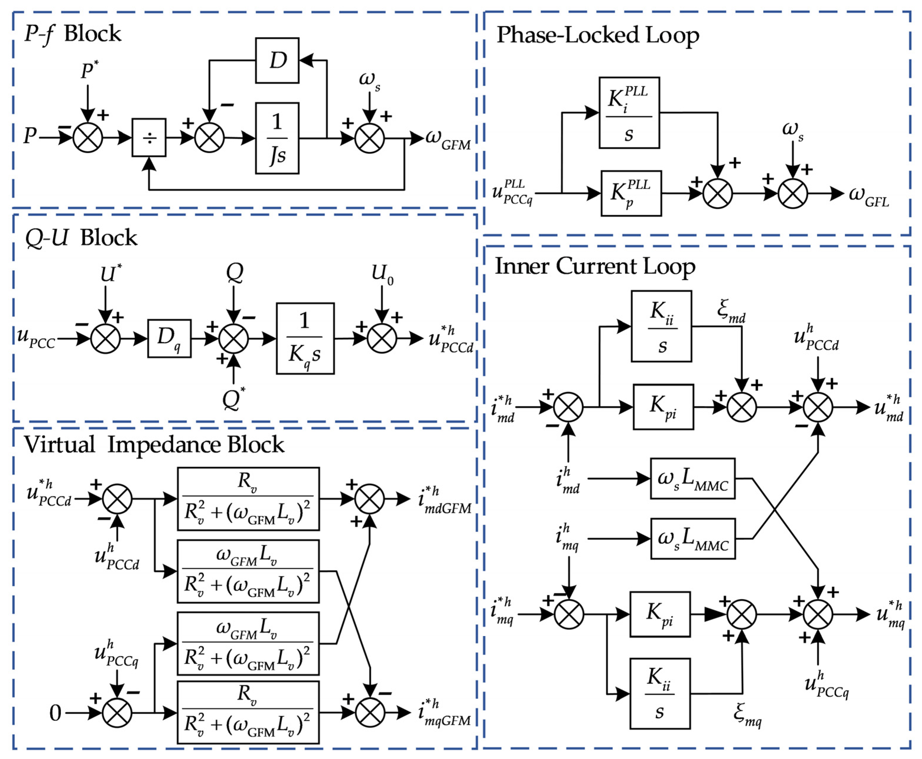
The detailed control blocks, including the phase-locked loop, the P-f block, the Q-U block, the virtual impedance block, and the inner current loop, are illustrated in Figure 2.

For the GFL synchronization, the PLL uses the q-axis PCC voltage in the PLL reference frame as the phase error, and the corresponding block can be expressed as follows:

$${\omega }_{GFL}={\dot{\theta }}_{GFL}={\omega }_s+K_p^{PLL}{u}_{PCCq}^{PLL}+K_i^{\mathrm{PLL}}{\displaystyle {\int }_0^t{u}_{PCCq}^{PLL}}\mathrm{d}\tau$$

(5)

where the superscript PLL denotes that the dq reference frame used in the expression is referenced to the phase angle provided by the PLL. $K_p^{PLL}$ and $K_i^{PLL}$ denote the proportional and integral gains of the PI regulators for the PLL.

For the GFL outer power loops, the d- and q-axis current references are generated as:

$$\left\{\begin{array}{l}{i}_{mdGFL}^{\ast h}=K_{pp}(P^{\ast }-P)+K_{ip}{\displaystyle \int (P^{\ast }-P)dt}\\ i_{mqGFL}^{\ast h}=K_{pq}(Q^{\ast }-Q)+K_{iq}{\displaystyle \int (Q^{\ast }-Q)dt}\end{array}\right.$$

(6)

where the superscript * denotes the reference value. $K_{pp}$ and $K_{ip}$ are the proportional and integral gains of the d-axis PI controller, and $K_{pq}$ and $K_{iq}$ are the proportional and integral gains of the q-axis PI controller.

For the GFM synchronization, the P-f loop emulates the inertial and primary frequency response characteristics, which can be expressed as follows:

$$\left\{\begin{array}{c}J{\dot{\omega }}_{\mathrm{GFM}}={\displaystyle \frac{P^{\star }-P}{{\omega }_{\mathrm{GFM}}}}-D({\omega }_{\mathrm{GFM}}-{\omega }_s)\\ {\dot{\theta }}_{\mathrm{GFM}}={\omega }_{\mathrm{GFM}}\end{array}\right.$$

(7)

where J and D denote the inertia and damping coefficients, respectively. ${\theta }_{GFM}$ is the synchronizing angle generated by the PSL, and ${\omega }_{GFM}$ is the angular frequency.

The Q-U loop regulates the PCC voltage magnitude by generating the d-axis PCC voltage reference:

$$u_{PCCd}^{\ast h}=U_0+{\displaystyle \frac{1}{K_q}}{\displaystyle \int \left[D_q\left(U^{\ast }-\left|u_{PCC}\right|\right)+\left(Q^{\ast }-Q\right)\right]}dt$$

(8)

where K_q is the reactive power integration coefficient, D_q is the reactive regulation coefficient, and $\left|u_{PCC}\right|$ denotes the PCC voltage magnitude, which is defined as:

$$\left|u_{PCC}\right|=\sqrt{{\left(u_{PCCd}^h\right)}^2+{\left(u_{PCCq}^h\right)}^2}$$

(9)

U₀ is the peak value of the rated system voltage, and U^* is the no-load electromotive force of the MMC.

The virtual impedance block emulates the stator resistance and synchronous reactance of a synchronous generator. In this paper, it is modeled in a quasi-steady-state manner without introducing additional state variables, and its effect is incorporated into the state-space model through algebraic coupling. The virtual-impedance-based current references are expressed as follows:

$$\left\{\begin{array}{l}{i}_{mdGFM}^{\ast h}={\displaystyle \frac{R_v\left(u_{PCCd}^{\ast h}-u_{PCCd}^h\right)+{\omega }_{\mathrm{GFM}}{L}_v\left(0-u_{PCCq}^h\right)}{R_v^2+{({\omega }_{\mathrm{GFM}}{L}_v)}^2}}\\ i_{mqGFM}^{\ast h}={\displaystyle \frac{-{\omega }_{\mathrm{GFM}}{L}_v\left(u_{PCCd}^{\ast h}-u_{PCCd}^h\right)+R_v\left(0-u_{PCCq}\right)}{R_v^2+{({\omega }_{\mathrm{GFM}}{L}_v)}^2}}\end{array}\right.$$

(10)

where R_v and L_v are the virtual resistance and virtual inductance, respectively.

Finally, the inner current control loop generates the MMC voltage references:

$$\left\{\begin{array}{l}{u}_{md}^{\ast h}=u_{PCCd}^h-{\omega }_s{L}_{MMC}{i}_{mq}^h+K_{pi}(i_{md}^{\ast h}-i_{md}^h)+K_{ii}{\xi }_d\\ u_{mq}^{\ast h}=u_{PCCq}^h+{\omega }_s{L}_{MMC}{i}_{md}^h+K_{pi}(i_{mq}^{\ast h}-i_{mq}^h)+K_{ii}{\xi }_q\end{array}\right.$$

(11)

with the integrator states governed by

$$\left\{\begin{array}{l}{\displaystyle \frac{d{\xi }_d}{dt}}=i_{md}^{\ast h}-i_{md}^h\\ {\displaystyle \frac{d{\xi }_q}{dt}}=i_{mq}^{\ast h}-i_{mq}^h\end{array}\right.$$

(12)

where $K_{pi}$ and $K_{ii}$ denote the proportional and integral gains of the PI regulators for the inner current control loop.

2.3. Hybrid Strategy

The synchronizing angles generated by the GFL and GFM schemes are fused through the hybrid coefficient $k_h$ to form the hybrid synchronizing angle ${\theta }_h$:

$${\theta }_h=k_h{\theta }_{GFL}+(1-k_h){\theta }_{GFM}={\displaystyle \int k_h{\omega }_{GFL}}dt+{\displaystyle \int \left(1-k_h\right)} {\omega }_{GFM}dt$$

(13)

In the dq reference frame, the current references generated by the current reference hybrid block can be expressed as follows:

$$\left\{\begin{array}{l}{i}_{md}^{\ast h}=k_h\cdot i_{mdGFL}^{\ast h}+(1-k_h)\cdot i_{mdGFM}^{\ast h}\\ i_{mq}^{\ast h}=k_h\cdot i_{mqGFL}^{\ast h}+(1-k_h)\cdot i_{mqGFM}^{\ast h}\end{array}\right.$$

(14)

where the superscript h denotes that the dq reference frame used in the expression is referenced to the hybrid synchronizing angle ${\theta }_h$.

In the above expressions, the hybrid coefficient $k_h$ takes values in the interval [0, 1]. A target hybrid coefficient $k_{h\_tar}$ is generated by the adaptive scheduling rule with the assessed short circuit ratio $\mathrm{S}\hat{\mathrm{C}}\mathrm{R}$ as input, which is defined as follows:

$$k_{h\_tar}=\left\{\begin{array}{l}0 , \mathrm{S}\hat{\mathrm{C}}\mathrm{R}\le {\mathrm{SCR}}_{weak}\\ {\displaystyle \frac{1}{1+e^{-(\mathrm{S}\hat{\mathrm{C}}\mathrm{R}-\frac{{\mathrm{SCR}}_{weak}+{\mathrm{SCR}}_{stiff}}{2})}}} , {\mathrm{SCR}}_{weak}<\mathrm{S}\hat{\mathrm{C}}\mathrm{R}\le {\mathrm{SCR}}_{stiff}\\ 1 , \mathrm{S}\hat{\mathrm{C}}\mathrm{R}>{\mathrm{SCR}}_{stiff}\end{array}\right.$$

(15)

where SCR_weak and SCR_stiff are defined as the critical values of extremely weak and extremely strong power grids, respectively.

In the above expressions, SĈR denotes the assessed short-circuit ratio at the PCC. In practice, SĈR can be obtained by both offline and online methods. As far as offline method is concerned, SĈR values of various system operation patterns can be calculated during grid planning and short-circuit studies [30]. The PCC short-circuit level is calculated under credible contingencies, network reconfiguration scenarios, and representative operating points and fault conditions. SĈR values can also be obtained through online measurement-based estimation [31], where the PCC voltage and current are used to estimate the grid Thévenin equivalent impedance ${\widehat{Z}}_{th}$, and SĈR is then computed as follows:

$$\mathrm{S}\hat{\mathrm{C}}\mathrm{R}={\displaystyle \frac{{\widehat{S}}_{sc}}{S_{rated}}}\approx {\displaystyle \frac{{\left|u_{PCC}\right|}^2}{S_{rated}\left|{\widehat{Z}}_{th}\right|}}$$

(16)

where ${\widehat{S}}_{sc}$ is the estimated short-circuit capacity at the PCC and $S_{rated}$ is the rated apparent power of the converter station. Under the grid equivalent adopted in this paper, ${\widehat{Z}}_{th}=j{\omega }_s{L}_s$.

It is noted that the proposed scheduling requires only an available value of SĈR and does not depend on a specific assessment implementation. Since this work focuses on severe transient current during large coefficient transitions under significant grid-strength changes, SĈR is updated in an event-triggered manner and held constant otherwise [32]. The SĈR inevitably differs from the actual SCR due to assessment error and update delay, and the impacts of these imperfections on the proposed strategy are further evaluated in Section 6.

The actual coefficient $k_h$ is obtained using the hybrid-coefficient regulating method, where ${\dot{k}}_h$ is produced in real time and integrated to update $k_h$. The enable logic activates the regulation only during coefficient transitions. Once $k_h$ reaches $k_{h\_tar}$, ${\dot{k}}_h$ is set to zero and $k_h$ remains constant in steady state. The detailed derivation and design of the regulating method are presented in Section 4 and Section 5.

Notably, the synchronizing angles ${\theta }_{GFL}$ and ${\theta }_{GFM}$ generated by GFL and GFM control are different, and the current references $i_{mdGFL}^{\ast h}$, $i_{mdGFM}^{\ast h}$, $i_{mqGFL}^{\ast h}$, $i_{mqGFM}^{\ast h}$ are also not identical. When there are pronounced discrepancies between ${\theta }_{GFL}$ and ${\theta }_{GFM}$, between $i_{mdGFL}^{\ast h}$ and $i_{mdGFM}^{\ast h}$, and between $i_{mqGFL}^{\ast h}$ and $i_{mqGFM}^{\ast h}$, changes in $k_h$ cause significant disturbances to the dq transformation and to the inner current loop. The faster $k_h$ varies, the stronger the disturbances are. Although the outer power loop commands remain slow adjustments, the converter still undergoes a transient process with a rapidly oscillating current.

2.4. Benchmarking of Representative GFL-GFM Coordination Strategies

To clarify the positioning of the proposed strategy,

Table 1. Benchmarking representative GFL-GFM coordination control strategies.

Control Strategies	Categories	Coordination Scopes	kh_tar Scheduling Manners	kh Transition Handling Mechanisms
Adaptive hybrid control with kh transition regulation	coefficient-based hybrid	synchronizing angle hybrid and current reference hybrid	SCR-adaptive	${\dot{k}}_h$-regulated
HCC-based hybrid control [21]	coefficient-based hybrid	terminal voltage/reference synthesis	Fixed	None
Hybrid-mode stability control [22]	coefficient-based hybrid	modulation (dq) combination	Fixed	None
SCR-adaptive hybrid control [23]	coefficient-based hybrid	synchronizing angle hybrid	SCR-adaptive	None (step-like update)
Seamless GFL/GFM switching control [27]	dual-mode switching	mode switching	-	seamless switching
Disturbance-free GFL/GFM switching control [28]	dual-mode switching	mode switching	-	disturbance-free switching

benchmarks representative GFL-GFM coordination strategies reported in Refs. [21,22,23,27,28]. The comparison focuses on the coordination category, the coordination scope within the control architecture, the scheduling manner of the target coefficient $k_{h\_tar}$, and the adopted transition handling mechanism.

As summarized in Table 1, coefficient-based hybridization strategies mainly focus on capability integration or small-signal stability enhancement, while coefficient-transition handling is typically not addressed. Dual-mode switching strategies handle discrete mode transitions but do not address transients caused by hybrid coefficient updates over intermediate values. In contrast, the proposed strategy shapes ${\dot{k}}_h$ to regulate the coefficient transition and achieve smooth online redistribution of GFL-GFM characteristics.

3. Small-Signal Modeling and Stability Analysis

To establish the small-signal stability of the proposed adaptive hybrid GFL-GFM control with a hybrid-coefficient regulating method under different grid strengths, the overall small-signal state–space model of the converter is established and linearized around the steady-state operating point corresponding to each SCR. For reference, the small-signal models of conventional GFL and GFM controls are also derived in a consistent manner, and their steady-state characteristics are compared with those of the hybrid control in the simulation studies.

Notably, the proposed hybrid-coefficient transition regulation is activated only during transient coefficient transitions. For small-signal analysis around a steady-state operating point, the scheduled target $k_{h\_tar}$ is constant and the enable logic deactivates the regulating action, enforcing ${\dot{k}}_h=0$. Hence, $k_h$ is constant at the operating point and can be treated as a parameter in the linearized model. Consequently, the state matrix and eigenvalues of the proposed strategy are identical to those of the baseline adaptive hybrid control without hybrid coefficient regulating method.

The linearized models can be given as:

$$\Delta {\dot{x}}_{GFL}=M_{GFL}\Delta x_{GFL}+N_{GFL}\Delta u$$

(17)

$$\Delta {\dot{x}}_{GFM}=M_{GFM}\Delta x_{GFM}+N_{GFM}\Delta u$$

(18)

$$\Delta {\dot{x}}_h=M_h\Delta x_h+N_h\Delta u$$

(19)

where $\Delta x_{GFL}$, $\Delta x_{GFM}$, and $\Delta x_h$ are the small-signal state vectors of the system under the GFL, GFM, and hybrid control modes, respectively, defined as $\Delta x_{GFL}={[\Delta i_{md},\Delta \hspace{0.33em}{i}_{mq},\hspace{0.33em}\Delta i_{mdGFL}^{\ast h},\hspace{0.33em}\Delta i_{mqGFL}^{\ast h},\hspace{0.33em}\Delta {\theta }_{\mathrm{GFL}},\hspace{0.33em}\Delta {\omega }_{GFL},\hspace{0.33em}\Delta {\xi }_{md},\hspace{0.33em}\Delta {\xi }_{mq}]}^{\mathrm{T}}$, $\Delta x_{GFM}={[\Delta i_{md}^h,\Delta \hspace{0.33em}{i}_{mq}^h,\hspace{0.33em}\Delta {\theta }_{GFM},\hspace{0.33em}\Delta {\omega }_{GFM},\hspace{0.33em}\Delta u_{PCCd}^{\ast h},\Delta {\xi }_{md},\hspace{0.33em}\Delta {\xi }_{mq}]}^{\mathrm{T}}$, $\Delta x_h={[\Delta i_{md}^h,\Delta \hspace{0.33em}{i}_{mq}^h,\Delta i_{mdGFL}^{\ast h},\Delta i_{mqGFL}^{\ast h},\Delta {\theta }_{\mathrm{GFL}},\Delta {\omega }_{GFL},\Delta {\theta }_{GFM},\Delta {\omega }_{GFM},\Delta u_{PCCd}^{\ast h},\Delta {\xi }_{md},\Delta {\xi }_{mq}]}^{\mathrm{T}}$, and $\Delta u={[\Delta P^{\ast },\Delta Q^{\ast }]}^{\mathrm{T}}$ denotes the perturbation of the input vector. The state–space matrices $M_{GFL}$ and $N_{GFL}$ are obtained by combining and linearizing Equations (1)–(4) and Equations (8)–(11). Similarly, $M_{GFM}$ and $N_{GFM}$ are obtained by combining and linearizing Equations (1)–(7), (10) and (11). For the hybrid control, $M_h$ and $N_h$ are obtained by combining and linearizing the complete set of equations in Equations (1)–(13).

A case study based on a 500 kV/2100 MW VSC-HVDC project is established, and the key parameters are summarized in

Table A1. Main parameters of the simulation model.

Symbol	Parameter	Value	Unit
Us	Grid line voltage	525	kV
ωs	Grid angular frequency	314	rad/s
Udc	DC-bus voltage	1.05 × 103	kV
Usm	Submodule dc-link voltage	2.18	kV
N	Number of submodules in a leg	480	-
C	Capacitance of the submodule	11	mF
LMMC	Leg inductance	80	mH
Pref	Active power reference	2.1 × 103	MW
Qref	Reactive power reference	0	MVar
Kpp	Proportional gain of the GFL d-axis outer-loop PI controller	8 × 10−6	-
Kip	Integral gain of the GFL d-axis outer-loop PI controller	4 × 10−4	-
Kpq	Proportional gain of the GFL q-axis outer-loop PI controller	8 × 10−6	-
Kiq	Integral gain of the GFL q-axis outer-loop PI controller	4 × 10−4	-
J	Virtual inertial	1.5 × 104	kg/m2
D	Damping coefficient	4 × 106	-
Kq	Reactive power integration coefficient	1.25 × 103	-
Dq	Reactive voltage regulation coefficient	31.25	-
U0	Peak value of the rated system voltage	4.29	kV
U*	No-load electromotive force of the MMC	4.29	kV
Rv	Virtual resistance	2	Ω
Lv	Virtual inductance	6	mH
Kpp	Proportional gain of current inner loop	30	-
Kii	Integral gain of current inner loop	3 × 103	-
SCRstiff	SCR threshold for extremely strong grid	16	-
SCRweak	SCR threshold for extremely weak grid	1.6	-
Kph	Proportional gain of the kh regulating method	1 × 104	-
Kih	Integral gain of the kh regulating method	3 × 103	-
$|{\dot{i}}_m{|}^{\ast }$	Reference value of current change rate	0	kA/s

. Based on the obtained state matrices $M_{GFL}$, $M_{GFM}$, and $M_h$, eigenvalue loci are plotted to compare the small-signal stability of the converter under different SCR conditions. The initial SCR is set to 16 with L_s = 26 mH, and it is reduced to 1.6 with L_s = 260 mH. All eigenvalue analyses were performed in MATLAB (The MathWorks, Natick, MA, USA), Release R2024b.

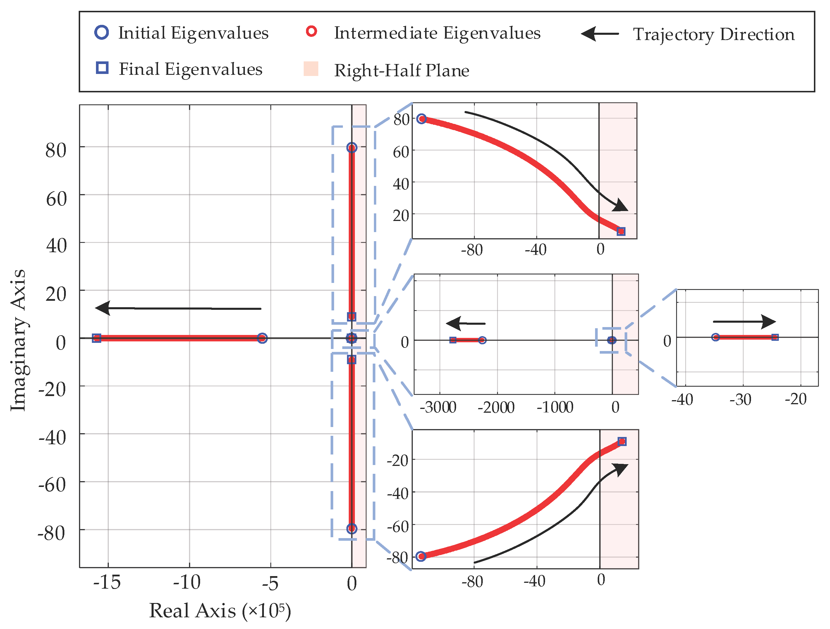
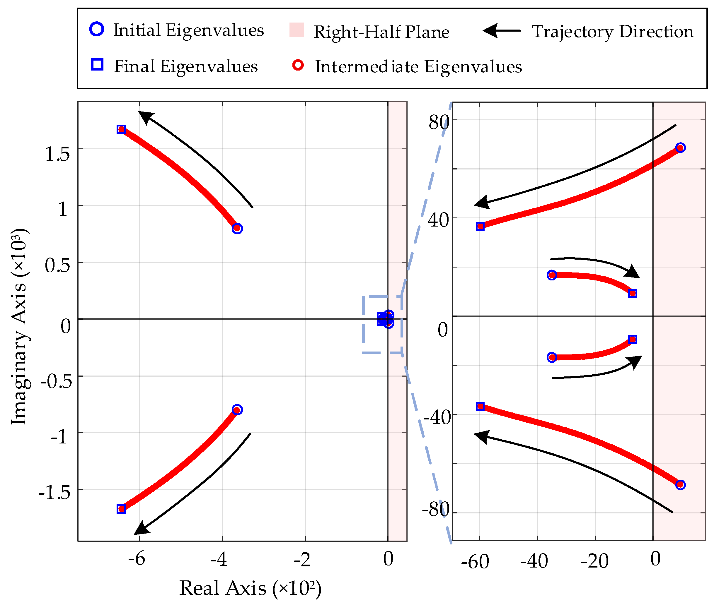
When the SCR decreases from 16 to 1.6, the eigenvalue loci of the converter under GFL control is plotted in Figure 3. It can be observed that a dominant complex-conjugate eigenvalue pair shifts rightward toward the imaginary axis when SCR decreases, indicating reduced damping. When SCR decreases below a critical value, this pair crosses the imaginary axis into the right-half plane, which signifies an oscillatory small-signal instability.

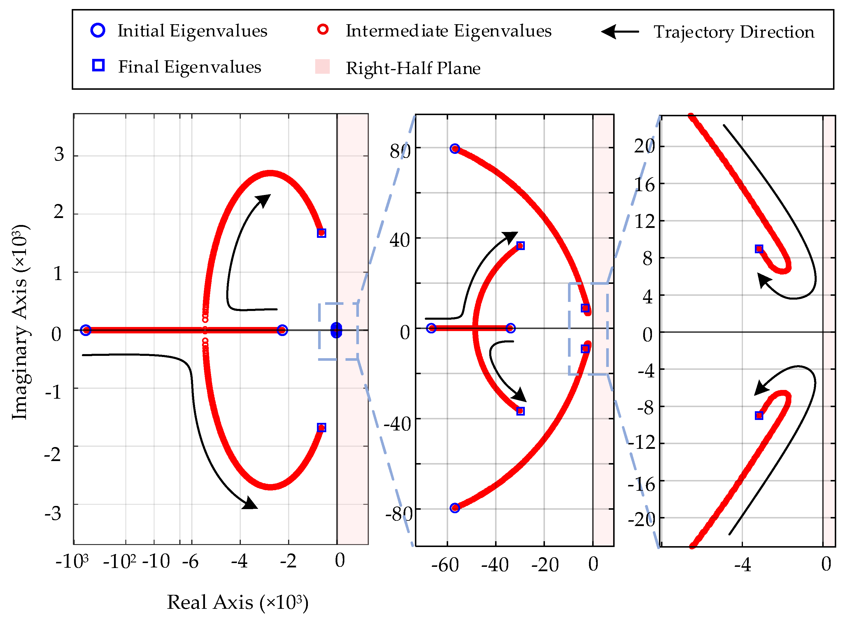
Figure 4 shows the eigenvalue loci of the converter under GFM control as SCR decreases from 16 to 1.6. It can be observed that a critical complex-conjugate pair lies in the right-half plane at SCR = 16, indicating an oscillatory small-signal instability. As SCR is reduced, this pair migrates leftward and crosses into the left-half plane, implying that the GFM-controlled converter becomes small-signal stable under weaker-grid conditions.

Figure 5 shows the eigenvalue loci of the converter under the proposed hybrid GFL–GFM control as SCR decreases from 16 to 1.6. With decreasing SCR, the hybrid coefficient $k_h$ is adjusted according to the proposed scheduling rule from 1 to 0, such that the control behavior gradually transitions from GFL-dominant to GFM-dominant. The critical eigenvalues initially move rightward, but then turn back and remain in the left-half plane throughout the entire SCR range.

To quantify the small-signal stability margin,

Table 2. Eigenvalue-based small-signal stability indices of the proposed strategy under varying SCR.

SCR	σmax (s−1) 1	ζmin 2	fcrit (Hz) 3
16	−56.8	0.58	12.67
10	−37.4	0.52	10.72
6	−16.1	0.42	6.86
1.6	−3.16	0.40	1.42
Worst case in 16–1.6	−1.71 at SCR = 2.8	0.29	1.18

¹ σ_max is the maximum real part among all eigenvalues. ² ζ_min denotes the minimum damping ratio among oscillatory eigenmodes. ³ f_crit is computed from the corresponding critical mode.

summarizes eigenvalue-based stability indices under representative SCR points and the worst case over SCR from 16 to 1.6. The maximum real part σ_max remains negative for all SCR, and the minimum damping ratio ζ_min stays positive, which provides a quantitative confirmation of small-signal stability. In addition, the corresponding critical-mode frequency f_crit indicates that the dominant oscillatory mode shifts toward a lower frequency as the grid becomes weaker.

Notably, since the hybrid coefficient regulating method is activated only during transient coefficient transitions and enforces ${\dot{k}}_h=0$ in steady state, the eigenvalue properties obtained here apply directly to the proposed strategy. Therefore, the proposed adaptive hybrid GFL-GFM control with the hybrid-coefficient regulating method is small-signal stable over the considered SCR range.

4. Influence Mechanism of Hybrid Coefficient Change Rate on Transient Current

To investigate how the change rate of the hybrid coefficient affects the transient current, mathematical models of the current derivative are first established in both the system synchronous and the hybrid synchronous dq reference frames. In the system synchronous frame, the d-axis is aligned with the grid voltage angle ${\theta }_s$, which is essentially independent of the hybrid coefficient. The state equations in this frame can therefore describe the dynamic relationships among the physical quantities in the main circuit. In contrast, in the hybrid synchronous frame, the d-axis is aligned with the hybrid synchronizing angle ${\theta }_h$, which is employed in the Park and inverse Park transformations of the hybrid GFL-GFM controller. Consequently, the dynamic relationships among the control variables are expressed in this frame. Since ${\theta }_h$ varies with the hybrid coefficient, the hybrid synchronous frame fluctuates accordingly, and the fluctuation is transmitted to the control system.

The converter current dynamics neglecting power losses can be expressed in the system synchronous reference frame as

$$\left\{\begin{array}{l}{\dot{i}}_{md}^s={\displaystyle \frac{1}{L_{eq}}}\left(u_{md}^s+{\omega }_s{L}_{eq}{i}_{mq}^s-u_{sd}^s\right)\\ {\dot{i}}_{mq}^s={\displaystyle \frac{1}{L_{eq}}}\left(u_{mq}^s-{\omega }_s{L}_{eq}{i}_{md}^s\right)\end{array}\right.$$

(20)

where the superscript s denotes that the reference frame is based on ${\theta }_s$. $u_{sd}^s$ is the system voltage, $u_{md}^s$ and $u_{mq}^s$ are the converter output voltages, $i_{md}^s$ and $i_{mq}^s$ are the converter currents, and ${\dot{i}}_{md}^s$ and ${\dot{i}}_{mq}^s$ represent the converter current change rates.

If the difference between the two synchronizing angles is defined as $\Delta \theta ={\theta }_s-{\theta }_h$, a vector ${(x_d,x_q)}^T$ can be written as

$$\left(\begin{array}{l}{x}_d^s\\ x_q^s\end{array}\right)=\left(\begin{array}{l}{x}_d^h\\ x_q^h\end{array}\right)\cdot P^{-1}({\theta }_h)\cdot P({\theta }_s)=\left(\begin{array}{l}{x}_d^h\cos \Delta \theta +x_q^h\sin \Delta \theta \\ -x_d^h\sin \Delta \theta +x_q^h\cos \Delta \theta \end{array}\right)$$

(21)

where $P$ and $P^{-1}$ denote the Park transformation matrix and its inverse, respectively.

According to Equation (21), substituting $u_{md}^s$ and $u_{mq}^s$ in Equation (20) with $u_{md}^h$ and $u_{mq}^h$ yields the following equation:

$$\left\{\begin{array}{l}{\dot{i}}_{md}^s={\displaystyle \frac{1}{L_{eq}}}\left(u_{md}^h\cos \Delta \theta +u_{mq}^h\sin \Delta \theta +{\omega }_s{L}_{eq}{i}_{mq}^s-u_{sd}^s\right)\\ {\dot{i}}_{mq}^s={\displaystyle \frac{1}{L_{eq}}}\left(-u_{md}^h\sin \Delta \theta +u_{mq}^h\cos \Delta \theta -{\omega }_s{L}_{eq}{i}_{md}^s\right)\end{array}\right.$$

(22)

By differentiating Equation (22), the following equation is obtained:

$$\left\{\begin{array}{l}{\ddot{i}}_{md}^s={\displaystyle \frac{1}{L_{eq}}}\left({\dot{u}}_{md}^h\cos \Delta \theta -u_{md}^h\sin \Delta \theta \cdot \Delta \dot{\theta }+\right.{\dot{u}}_{mq}^h\sin \Delta \theta +u_{mq}^h\cos \Delta \theta \cdot \Delta \dot{\theta }+\left.{\omega }_s{L}_{eq}{\dot{i}}_{mq}^s\right)\\ {\ddot{i}}_{mq}^s={\displaystyle \frac{1}{L_{eq}}}\left(-{\dot{u}}_{md}^h\sin \Delta \theta -u_{md}^h\cos \Delta \theta \cdot \Delta \dot{\theta }+\right.{\dot{u}}_{mq}^h\cos \Delta \theta -u_{mq}^h\sin \Delta \theta \cdot \Delta \dot{\theta }-\left.{\omega }_s{L}_{eq}{\dot{i}}_{md}^s\right)\end{array}\right.$$

(23)

Equation (23) indicates that the transient current is affected by both the fluctuation of the synchronizing angle difference and the fluctuation of the converter voltage. The change rate of the synchronizing angle originates from the synchronizing angle hybrid block, which can be expressed as follows:

$$\Delta \dot{\theta }={\dot{\theta }}_s-{\dot{\theta }}_h={\omega }_s-{\omega }_{GFM}-{\dot{k}}_h\left({\theta }_{GFL}-{\theta }_{GFM}\right)-k_h\left({\omega }_{GFL}-{\omega }_{GFM}\right)$$

(24)

With the reasonable assumption of an ideal converter, its voltages $u_{md}^h$ and $u_{mq}^h$ can be regarded as equal to the voltage references $u_{md}^{h\ast }$ and $u_{mq}^{h\ast }$. Based on the inner current loop, the converter voltages can be expressed as follows:

$$\left\{\begin{array}{l}{u}_{md}^{h\ast }=u_{PCCd}^h-{\omega }_s{L}_{MMC}{i}_{mq}^h+K_{pi}(i_{md}^{\ast h}-i_{md}^h)+K_{ii}{\displaystyle \int (i_{md}^{\ast h}-i_{md}^h)dt}\\ u_{mq}^{h\ast }=u_{PCCq}^h+{\omega }_s{L}_{MMC}{i}_{md}^h+K_{pi}(i_{mq}^{\ast h}-i_{mq}^h)+K_{ii}{\displaystyle \int (i_{mq}^{\ast h}-i_{mq}^h)dt}\end{array}\right.$$

(25)

Considering that the outer power control loop is assigned a much larger time scale than the inner current control loop and that the PCC voltages vary much more slowly than converter currents, the differential of converter voltages can be written as

$$\left\{\begin{array}{l}{\dot{u}}_{md}^h=-{\omega }_s{L}_{MMC}{\dot{i}}_{mq}^h+K_{ii}(i_{md}^{\ast h}-i_{md}^h)+K_{pi}\left[\left(i_{mdGFL}^{\ast h}-i_{mdGFM}^{\ast h}\right){\dot{k}}_h-{\dot{i}}_{md}^h\right]\\ {\dot{u}}_{mq}^h={\omega }_s{L}_{MMC}{\dot{i}}_{md}^h++K_{ii}(i_{mq}^{\ast h}-i_{mq}^h)+K_{pi}\left[\left(i_{mqGFL}^{\ast h}-i_{mqGFM}^{\ast h}\right){\dot{k}}_h-{\dot{i}}_{mq}^h\right]\end{array}\right.$$

(26)

Substituting Equation (3) into Equation (26) yields

$$\left\{\begin{array}{c}{\dot{u}}_{md}^h=K_{pi}\left(i_{mdGFL}^{\ast h}-i_{mdGFM}^{\ast h}\right){\dot{k}}_h-{\displaystyle \frac{K_{pi}}{L_{eq}}}\left(u_{md}^h-u_{sd}^h\right)-{\displaystyle \frac{{\omega }_s{L}_{MMC}}{L_{eq}}}\left(u_{mq}^h-u_{sq}^h\right)+\left({\omega }_h{\omega }_s{L}_{MMC}-K_{ii}\right)i_{md}^h-K_{pi}{\omega }_h{i}_{mq}^h+K_{ii}{i}_{md}^{\ast h}\\ {\dot{u}}_{mq}^h=K_{pi}\left(i_{mqGFL}^{\ast h}-i_{mqGFM}^{\ast h}\right){\dot{k}}_h-{\displaystyle \frac{K_{pi}}{L_{eq}}}\left(u_{mq}^h-u_{sq}^h\right)+\left({\omega }_h{\omega }_s{L}_{MMC}-K_{ii}\right)i_{mq}^h+K_{pi}{\omega }_h{i}_{md}^h+K_{ii}{i}_{mq}^{\ast h}+{\displaystyle \frac{{\omega }_s{L}_{MMC}}{L_{eq}}}\left(u_{md}^h-u_{sd}^h\right)\end{array}\right.$$

(27)

From Equations (23) and (24), it can be observed that the change rate of the hybrid coefficient affects the transient current through two paths. On the one hand, it directly contributes to the change rate of the synchronizing angle difference in the hybrid synchronizing angle block. On the other hand, it affects the change rate of the current reference, and this effect is transmitted to the change rate of the converter voltage through the proportional gain of the inner current loop PI controller.

By substituting Equations (20), (24) and (27) into Equation (23), the dynamic equation of the current change rate of the converter can be expressed as follows:

$$\left\{\begin{array}{l}{\ddot{i}}_{md}^s=A_d(t){\dot{k}}_h+B_d(t)\\ {\ddot{i}}_{mq}^s=A_q(t){\dot{k}}_h+B_q(t)\end{array}\right.$$

(28)

where $A_d(t)$, $A_q(t)$, $B_d(t)$, and $B_q(t)$ can be expressed as follows:

$$\left\{\begin{array}{ll}{A}_d& ={\displaystyle \frac{1}{L_{eq}}}[K_{pi}\left(i_{mdGFL}^{\ast h}-i_{mdGFM}^{\ast h}\right)\cos \Delta \theta +K_{pi}\left(i_{mqGFL}^{\ast h}-i_{mqGFM}^{\ast h}\right)\sin \Delta \theta +\left(u_{md}^h\sin \Delta \theta -u_{mq}^h\cos \Delta \theta \right)\left({\theta }_{GFL}-{\theta }_{GFM}\right)]\\ A_q& ={\displaystyle \frac{1}{L_{eq}}}\left[-K_{pi}\left(i_{mdGFL}^{\ast h}-i_{mdGFM}^{\ast h}\right)\sin \Delta \theta +\right.K_{pi}\left(i_{mqGFL}^{\ast h}-i_{mqGFM}^{\ast h}\right)\cos \Delta \theta +\left.\left(u_{md}^h\cos \Delta \theta +u_{mq}^h\sin \Delta \theta \right)\left({\theta }_{GFL}-{\theta }_{GFM}\right)\right]\\ B_d& ={\displaystyle \frac{1}{L_{eq}}}\left\{\left[{\displaystyle \frac{K_{pi}}{L_{eq}}}\left(u_{md}^h-u_{sd}^h\right)+{\displaystyle \frac{{\omega }_s{L}_{MMC}}{L_{eq}}}\left(u_{mq}^h-u_{sq}^h\right)\right]\cos \Delta \theta +\right.\left[{\displaystyle \frac{{\omega }_s{L}_{MMC}}{L_{eq}}}\left(u_{md}^h-u_{sd}^h\right)-{\displaystyle \frac{K_{pi}}{L_{eq}}}\left(u_{mq}^h-u_{sq}^h\right)\right]\sin \Delta \theta +\\ & \left[\left({\omega }_h{\omega }_s{L}_{MMC}-K_{ii}\right)\cos \Delta \theta +K_{pi}{\omega }_h\sin \Delta \theta \right]i_{md}^h+\left[\left({\omega }_h{\omega }_s{L}_{MMC}-K_{ii}\right)\sin \Delta \theta -K_{pi}{\omega }_h\cos \Delta \theta \right]i_{mq}^h-\\ & K_{ii}\left(i_{md}^{\ast h}\cos \Delta \theta +i_{mq}^{\ast h}\sin \Delta \theta \right)+{\omega }_s\left(u_{mq}^s-{\omega }_s{L}_{eq}{i}_{md}^s\right)-\left(u_{md}^h\sin \Delta \theta -u_{mq}^h\cos \Delta \theta \right)\left[\left.{\omega }_s-{\omega }_{GFM}-\left.k_h\left({\omega }_{GFL}-{\omega }_{GFM}\right)\right]\right\}\right.\\ B_q& ={\displaystyle \frac{1}{L_{eq}}}\left\{\left[{\displaystyle \frac{K_{pi}}{L_{eq}}}\left(u_{md}^h-u_{sd}^h\right)+{\displaystyle \frac{{\omega }_s{L}_{MMC}}{L_{eq}}}\left(u_{mq}^h-u_{sq}^h\right)\right]\sin \Delta \theta +\right.\left[{\displaystyle \frac{{\omega }_s{L}_{MMC}}{L_{eq}}}\left(u_{md}^h-u_{sd}^h\right)-{\displaystyle \frac{K_{pi}}{L_{eq}}}\left(u_{mq}^h-u_{sq}^h\right)\right]\cos \Delta \theta +\\ & \left[\left({\omega }_h{\omega }_s{L}_{MMC}-K_{ii}\right)\sin \Delta \theta +K_{pi}{\omega }_h\cos \Delta \theta \right]i_{md}^h+\left[\left({\omega }_h{\omega }_s{L}_{MMC}-K_{ii}\right)\cos \Delta \theta -K_{pi}{\omega }_h\sin \Delta \theta \right]i_{mq}^h+\\ & K_{ii}\left(i_{md}^{\ast h}\sin \Delta \theta +i_{mq}^{\ast h}\cos \Delta \theta \right)+{\omega }_s\left(u_{md}^s+{\omega }_s{L}_{eq}{i}_{mq}^s-u_{sd}^s\right)-\left(u_{md}^h\cos \Delta \theta +u_{mq}^h\sin \Delta \theta \right)\left[{\omega }_s-{\omega }_{GFM}-\left.\left.k_h\left({\omega }_{GFL}-{\omega }_{GFM}\right)\right]\right\}\right.\end{array}\right.$$

(29)

From Equation (29), the change rate of the converter current magnitude, $|{\dot{i}}_m|$, is directly affected by the hybrid coefficient change rate ${\dot{k}}_h$; it is also influenced by controller parameters, primary circuit parameters, and the instantaneous values of voltages and currents. The variation profile of $k_h$ differs according to different hybrid GFL-GFM control strategies, and so does its effect on the current change rate. For example, under mode-switching control or hybrid control without a ${\dot{k}}_h$ regulator, ${\dot{k}}_h$ tends to infinity at the moment SCR changes, which in turn causes the current change rate to soar and induces large transient current fluctuations.

5. Hybrid Coefficient Regulating Method

Although it is extremely difficult to analytically solve the hybrid coefficient change rate, ${\dot{k}}_h$, from the preceding mathematical model, it reveals that, during the transient process, ${\dot{k}}_h$ affects the current change rate directly, which provides the possibility of shaping the transient current. However, its regulating method varies with different control strategies and operating conditions. An excessively large ${\dot{k}}_h$ will lead to large current fluctuations and unsatisfactory suppression effects, whereas an excessively small ${\dot{k}}_h$ may prolong the transition time between GFL and GFM, affecting system stability. Therefore, this paper proposes a hybrid coefficient regulating method based on the state equations of the current change rate, thus providing a reasonable ${\dot{k}}_h$ with the aim of suppressing the transient current.

As far as a short transient process of MMC is concerned, the total current magnitude is usually of greater concern than the individual d- or q-axis component. The magnitude of the converter current vector is calculated as follows:

$$|i_m|=\sqrt{{\left(i_{md}^s\right)}^2+{\left(i_{mq}^s\right)}^2}$$

(30)

Based on Equations (20) and (28), the dynamics of the change rate of $|i_m|$, i.e., the second derivative of the above Equation (30), can be easily derived as follows:

$$|{\ddot{i}}_m|={\displaystyle \frac{d^2|i_m|}{d{t}^2}}=A(t){\dot{k}}_h+B(t)$$

(31)

where $A(t)$ denotes the equivalent time-varying gain of ${\dot{k}}_h$ and $B(t)$ represents the terms independent of ${\dot{k}}_h$. Their expressions are as follows:

$$\left\{\begin{array}{l}A(t)={\displaystyle \frac{i_{md}^s}{|i_m|}}{A}_d(t)+{\displaystyle \frac{i_{mq}^s}{|i_m|}}{A}_q(t)\\ B(t)={\displaystyle \frac{i_{md}^s}{|i_m|}}{B}_d(t)+{\displaystyle \frac{i_{mq}^s}{|i_m|}}{B}_q(t)+{\displaystyle \frac{{(u_{md}^s-{\omega }_s{L}_{eq}{i}_{mq}^s)}^2+{(u_{mq}^s+{\omega }_s{L}_{eq}{i}_{md}^s-u_{sd}^s)}^2}{L_{eq}^2\cdot |i_m|}}-\\ {\displaystyle \frac{{\left[i_{md}^s(u_{mq}^s+{\omega }_s{L}_{eq}{i}_{md}^s-u_{sd}^s)+i_{mq}^s(u_{md}^s-{\omega }_s{L}_{eq}{i}_{mq}^s)\right]}^2}{L_{eq}^2\cdot |i_m{|}^3}}\end{array}\right.$$

(32)

Equation (32) can be regarded as a linear time-varying state equation with the current change rate $|{\dot{i}}_m|$ as the state variable and ${\dot{k}}_h$ as the control input. Considering the complexity of the implementation and practical applicability, a PI form is adopted based on its simple structure, clear gain interpretation, and reasonable robustness to modeling errors. Accordingly, the second derivative of the converter current magnitude $|{\ddot{i}}_m|$ is represented as a PI function of the error of the current change rate. By combining this desired closed-loop relation with the physical model in Equation (32), the required hybrid coefficient change rate ${\dot{k}}_h$ can be obtained from the second derivative of the converter current magnitude. In this formulation, $B(t)$ represents the inherent current acceleration caused by the converter and network dynamics when $k_h$ is kept constant, and is used as a feedforward term to compensate this effect. $A(t)$ characterizes the equivalent gain from ${\dot{k}}_h$ to $|{\ddot{i}}_m|$, and normalizing by $A(t)$ keeps the magnitude and dynamic characteristics of the regulation approximately consistent under different operating conditions. 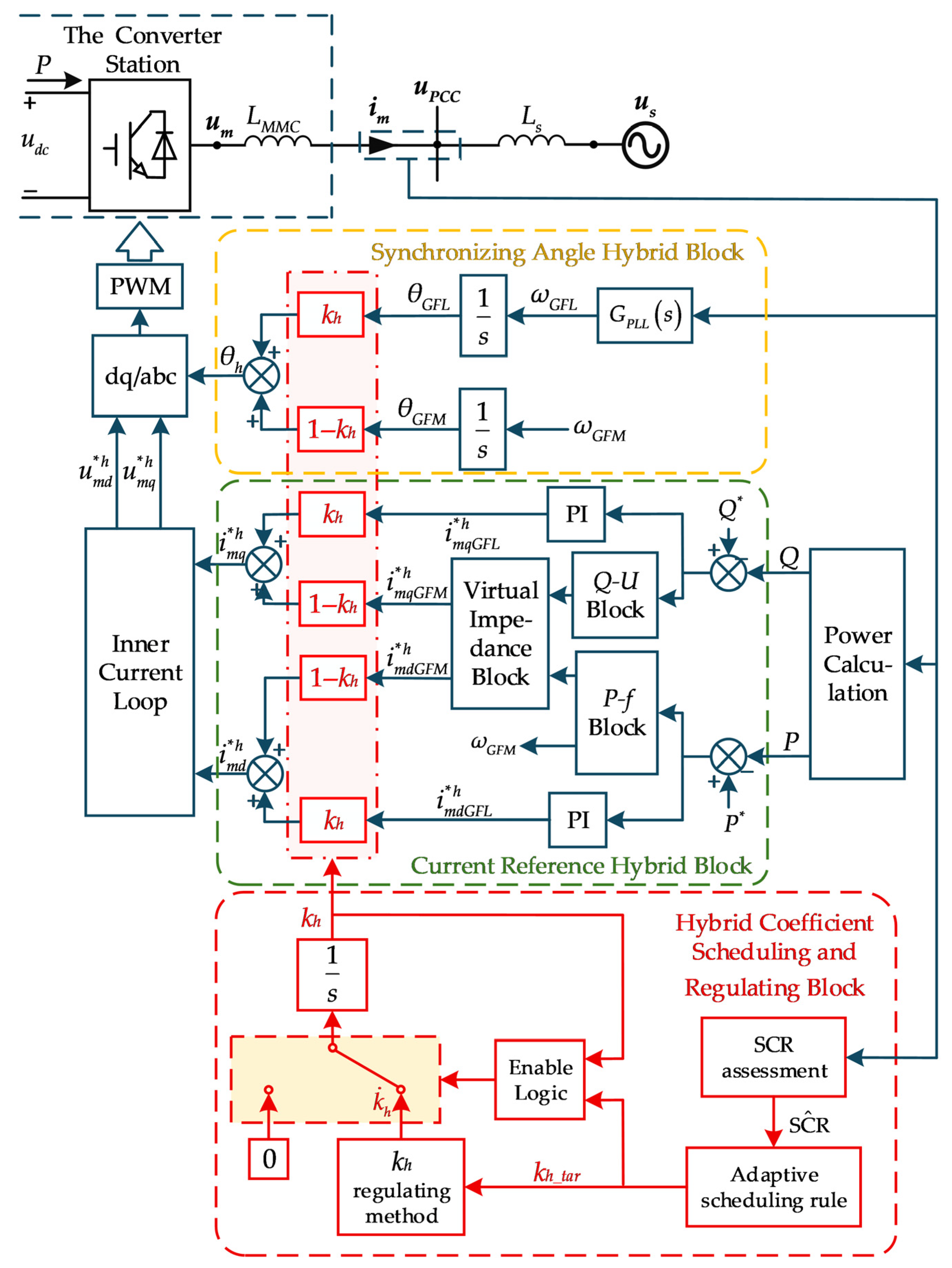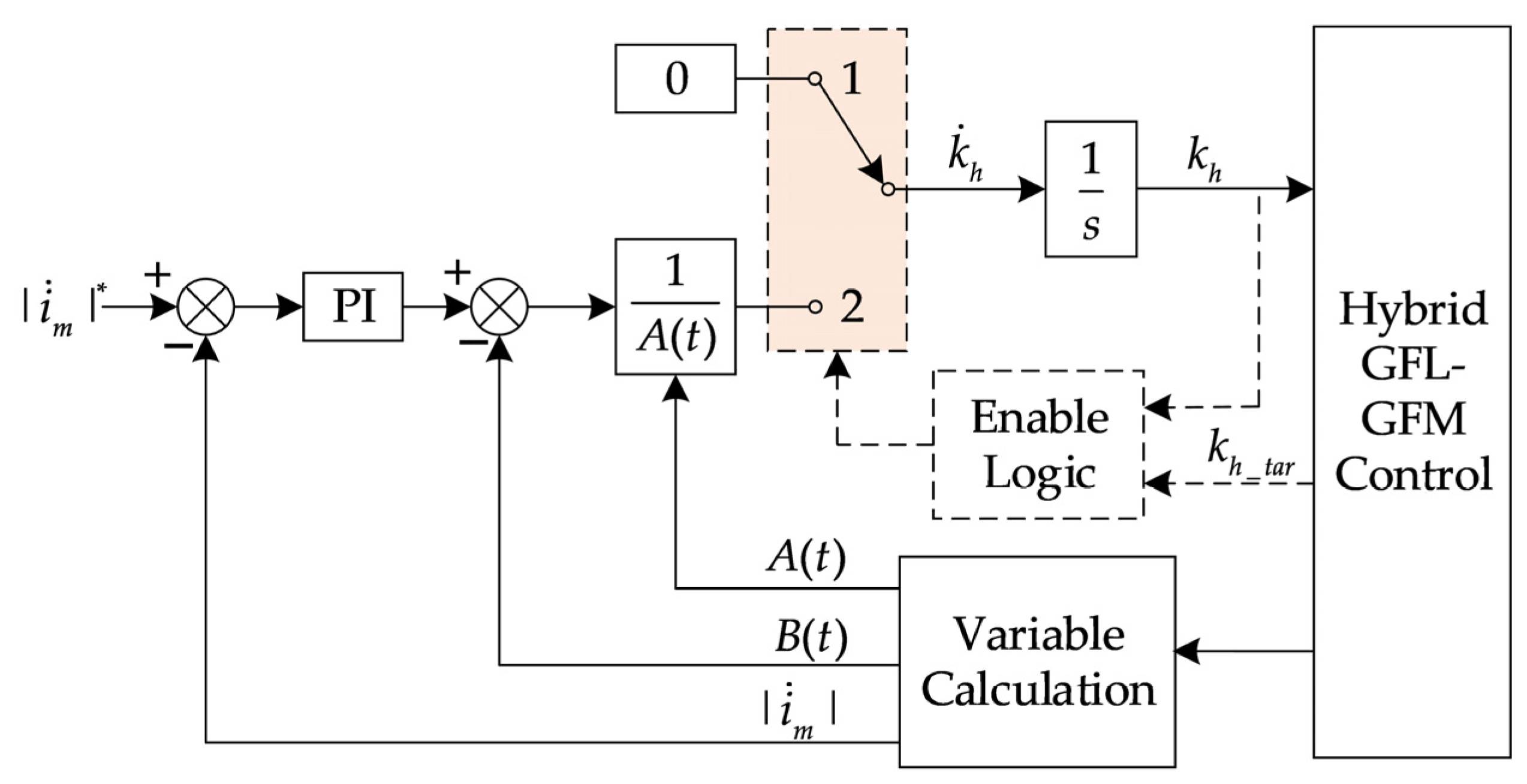Based on the above analysis, a closed-loop regulator can be designed to output an appropriate ${\dot{k}}_h$ in real time so as to suppress the transient current. The corresponding control structure is illustrated in Figure 6.

The enable logic block makes the regulator take effect only when the $k_{h\_tar}$ value changes, which means the converter enters a transient period. Under steady-state operation, this block chooses State 1 so that ${\dot{k}}_h$ remains at zero and $k_h$ retains its original value. When an SCR change calls a new hybrid coefficient value for $k_{h\_tar}$ generated from the hybrid control strategy, this block chooses State 2 to start ${\dot{k}}_h$ regulation.

In addition, as the outputs of the variable calculation block, $A(t)$ and $B(t)$ can be calculated in real time according to Equation (32), and $|{\dot{i}}_m|$ can be computed by taking the derivative of Equation (30) and substituting Equation (20) to eliminate the current derivatives; the result is written as follows:

$$|{\dot{i}}_m|={\displaystyle \frac{1}{L_{eq}\cdot |i_m|}}\left[i_{md}^s(u_{md}^s+{\omega }_s{L}_{eq}{i}_{md}^s-u_{sd}^s)+\left.i_{mq}^s(u_{md}^s-{\omega }_s{L}_{eq}{i}_{mq}^s)\right]\right.$$

(33)

With a specified value of $|{\dot{i}}_m{|}^{\ast }$, the reference of the transient current change rate, the error between $|{\dot{i}}_m{|}^{\ast }$ and $|{\dot{i}}_m|$ is dealt with by the PI regulator. Its output subtracts the feedforward $B(t)$ and is then divided by $A(t)$ to obtain the required $k_h$. After integration, $k_h$ is updated and assigned to the synchronizing angle hybrid block and the current reference hybrid block. Thus, the current change rate is controlled by a closed loop in which ${\dot{k}}_h$ serves as the controlling variable. Until the value of $k_h$ reaches $k_{h\_tar}$, the switching decision block turns back to State 1 and the converter enters a new steady-state operation.

For routine operating requirements, the reference value of the transient current change rate $|{\dot{i}}_m{|}^{\ast }$ is set to zero to effectively suppress current fluctuations. This choice is consistent with the steady-state condition, since the converter current in the synchronously rotating reference frame is constant and the desired current change rate is zero. In this work, the current change rate is introduced to suppress current fluctuations during the hybrid coefficient transition, rather than enforcing a nonzero current change rate. Therefore, $|{\dot{i}}_m{|}^{\ast }=0$ helps suppress oscillations and abrupt current variations, which reduces current overshoot and improves the settling time. With field operation demands considered, $|{\dot{i}}_m{|}^{\ast }$ might be appropriately relaxed to improve converter dynamic performance, which may lead to larger transient current fluctuations.

Additionally, the proportional gain K_ph and integral gain K_ih of the PI controller are determined as follows. First, based on the admissible overshoot and the target settling time of the converter current magnitude, a desired transient response of the current change rate loop is specified. The loop is then tuned by approximating it as a well-damped second-order system, which provides initial values of K_ph and K_ih and ensures that the corresponding closed-loop bandwidth lies between the bandwidths of the outer power controllers and the inner current controller, so that a reasonable separation of control time scales is maintained [33]. Next, time-domain simulations are carried out under several representative SCR conditions, and K_ph and K_ih are slightly adjusted so that the transient performance metrics, including current overshoot and settling time, satisfy the design requirements for all cases. The final gain values are listed in Table A1.

6. Simulation Verification

To validate the proposed adaptive hybrid GFL–GFM control with a hybrid-coefficient regulating method, time-domain simulations are conducted on a 500 kV/2100 MW MMC-based VSC–HVDC station. The grid strength is emulated by varying the SCR, and the main parameters of the simulation model are listed in Table A1. All time-domain simulations were carried out in Simulink (The MathWorks, Natick, MA, USA), Release R2024b.

In the following, the baseline strategy refers to the SCR-adaptive hybrid control without the proposed hybrid-coefficient transition regulation, where $k_h$ varies adaptively with SCR and is updated directly toward $k_{h\_tar}$, serving as the benchmark for evaluating the benefit of the transition regulation.

The simulation studies are organized as follows. First, the grid adaptability of the baseline is compared with conventional GFL and GFM controls over a wide SCR range. Then, the effectiveness of the hybrid coefficient regulating method is verified by comparing the proposed strategy with the baseline under SCR variations. Finally, the robustness of the proposed strategy against variations in key system parameters is evaluated.

6.1. Comparison of Grid Adaptability of GFL, GFM, and Baseline Adaptive Hybrid Control

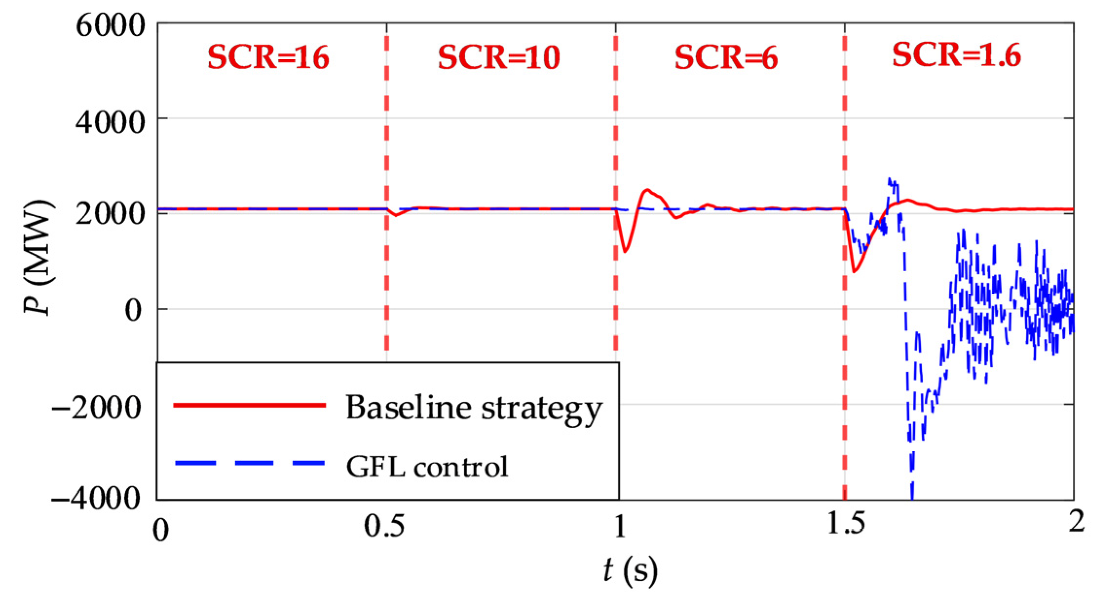
At first, the SCR is initialized to 16 and steps down in sequence to 10, 6, and 1.6 at 0.5 s, 1 s, and 1.5 s. The active power responses of the converter under GFL control and baseline strategy are shown by the dashed blue line and the solid red line in Figure 7, respectively. The converter operates stably when the SCR is high. However, as the SCR decreases, the disturbances cause increasingly large power oscillations, and the grid becomes extremely weak when the SCR falls to 1.6. Under this condition, GFL control cannot maintain stability in the converter, whereas the baseline adaptive hybrid control is capable of maintaining smooth active power output during the entire process of decreasing SCR.

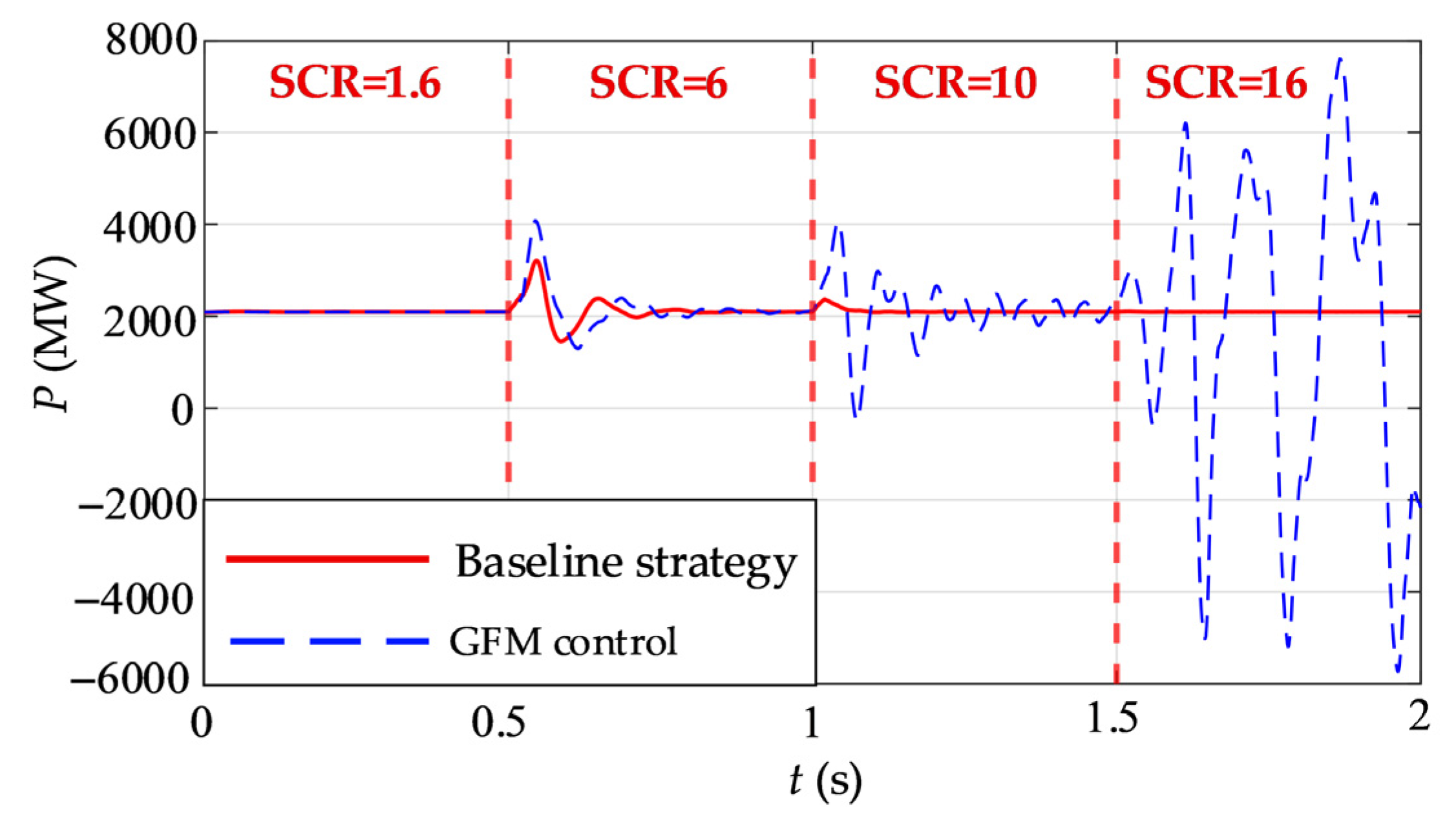
Similarly, the SCR is initialized to 1.6 and steps up in sequence to 6, 10, and 16 at 0.5 s, 1 s, and 1.5 s. The active power responses of the converter under GFM control and strategy are shown by the dashed blue line and the solid red line in Figure 8, respectively. In this case, the converter operates stably when the SCR is low. As the SCR increases, the disturbances cause increasingly noticeable power oscillations, and GFM control is unable eliminate the low-frequency oscillations in a short time. The grid becomes extremely strong when the SCR rises to 16. Under this condition, GFM control cannot keep the converter stable, whereas the baseline adaptive hybrid control is capable of maintaining smooth active-power output over the entire process of increasing SCR.

The results above demonstrate that the baseline adaptive hybrid control can exhibit grid-following and grid-forming characteristics depending on grid strength, thereby achieving stable operation over a wide SCR range and showing strong adaptability to varying grid strengths.

6.2. Effect Verification of Hybrid-Coefficient Transition Regulation

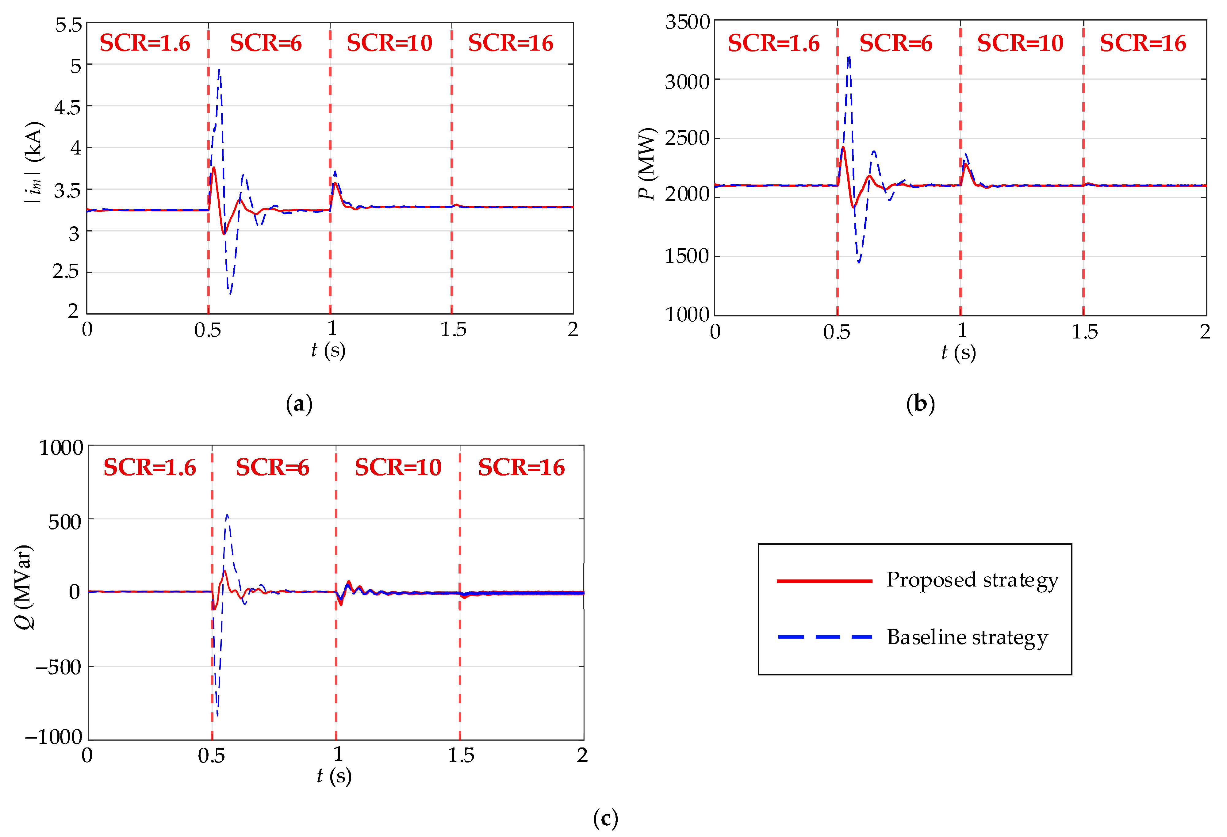
As demonstrated in Section 6.1, the baseline SCR-adaptive hybrid control maintains stable operation over a wide SCR range. However, during the transient process caused by sudden changes in SCR, the active power of the converter exhibits large oscillations, especially when the grid is weak. Therefore, transient current suppression in the hybrid control is necessary.

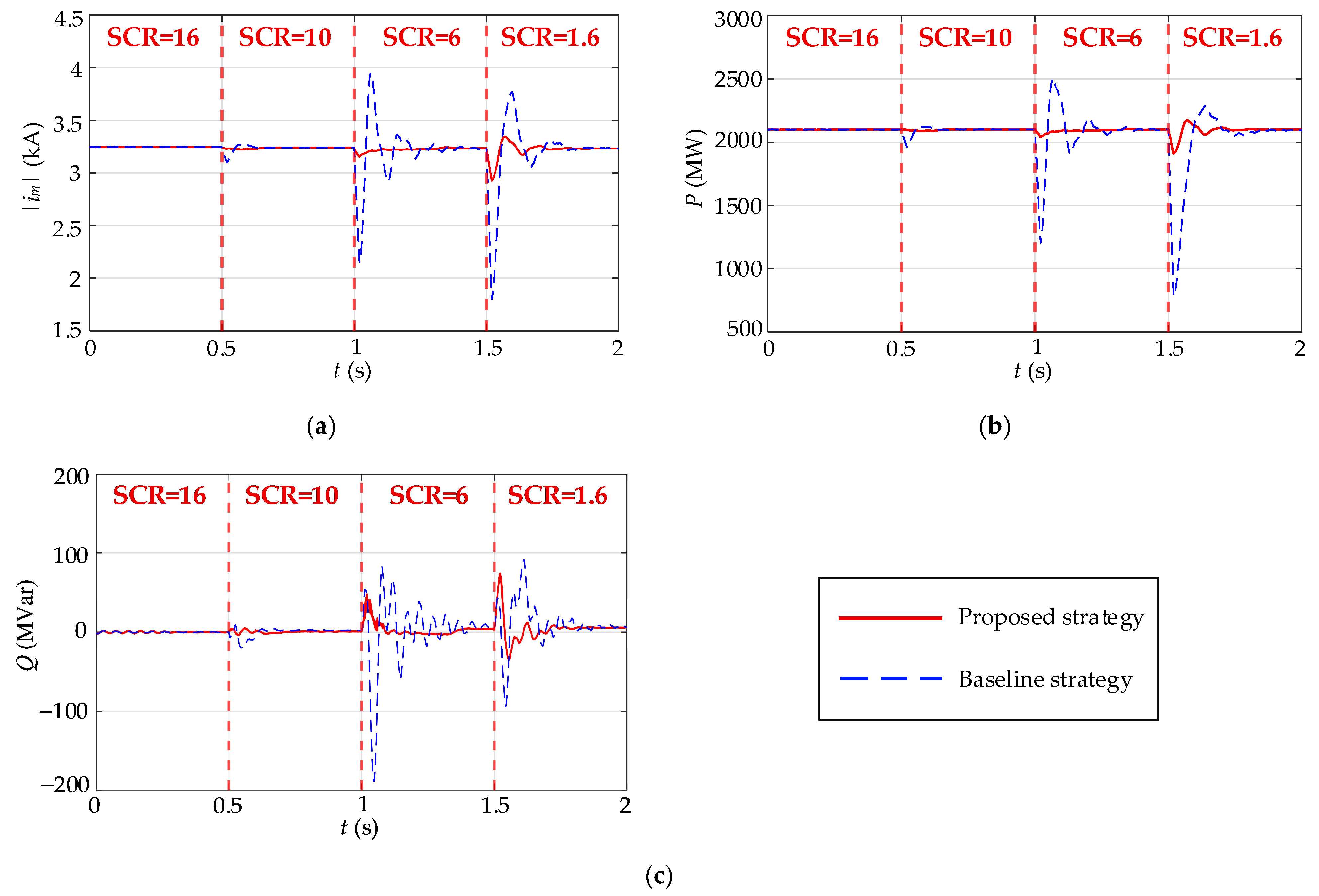
Similarly, the SCR value is set to decrease sequentially from 16 to 10, 6, and 1.6 at 0.5 s, 1 s, and 1.5 s. Figure 9 and Figure 10 show the simulation results of the hybrid control under the baseline and proposed strategies during SCR dives.

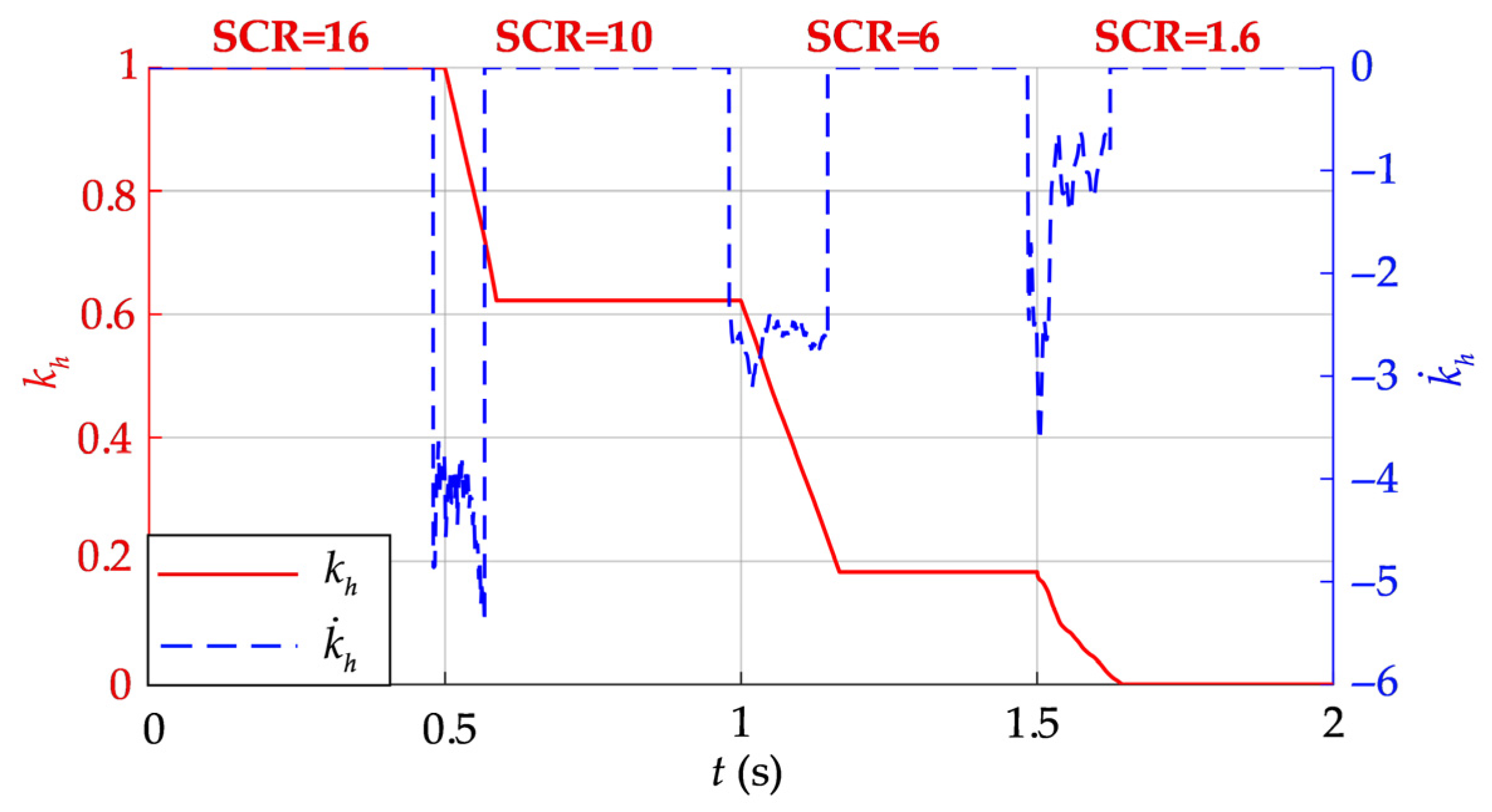
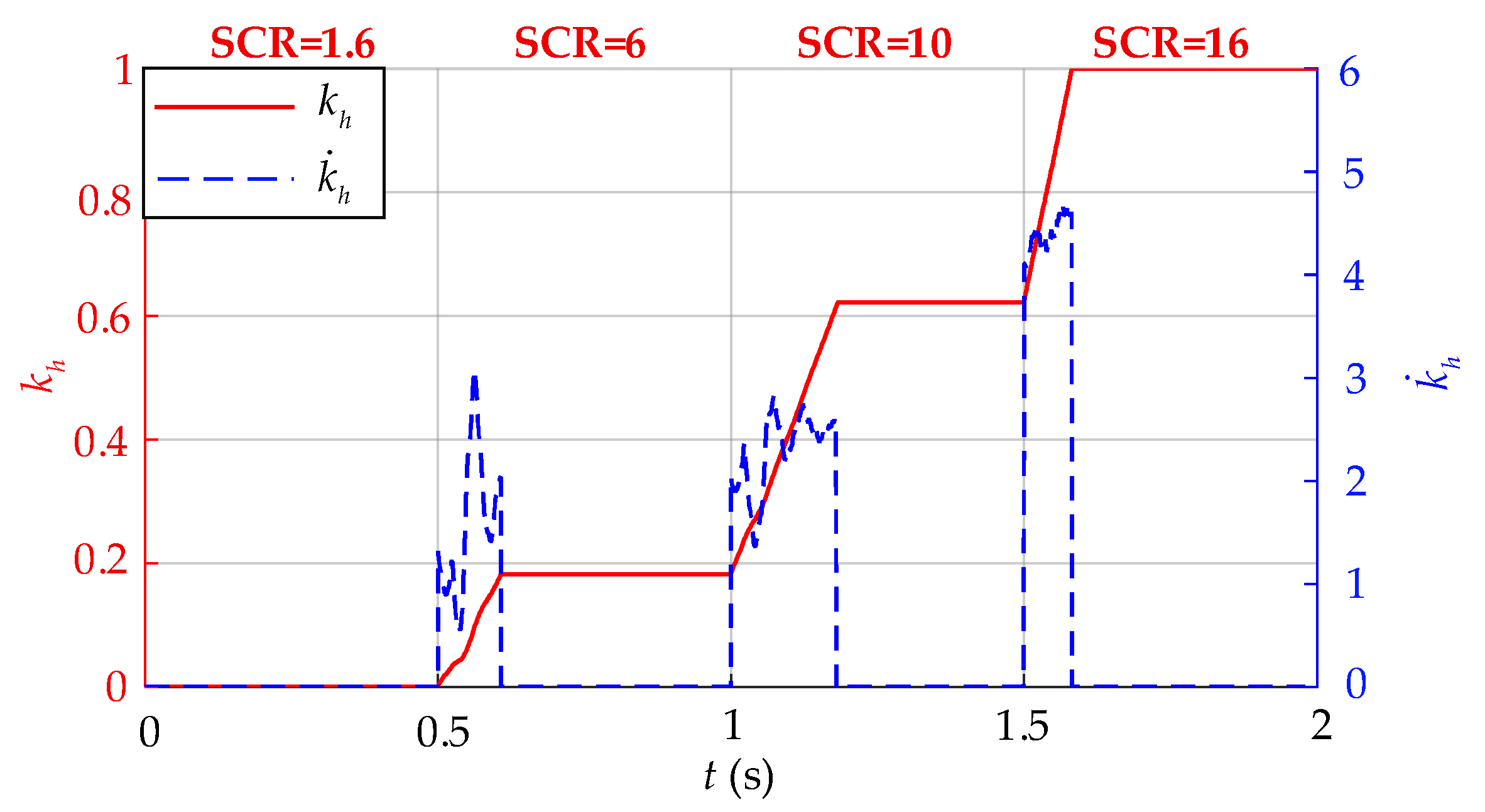
Figure 9 shows the curves of the hybrid coefficient $k_h$ and its change rate ${\dot{k}}_h$ with the proposed hybrid coefficient regulating method during SCR dives. $k_h$ and ${\dot{k}}_h$ are represented by the solid red line and the dashed blue line, respectively. It can be observed that each time SCR changes, $k_h$ exhibits no sudden jump. Instead, it transits toward the target value along $k_h$ generated by the regulator in real time. Once $k_h$ reaches the target value, ${\dot{k}}_h$ becomes zero. It is also clear that the amplitude of ${\dot{k}}_h$ diminishes with reductions in SCR. When SCR decreases from 16 to 10, ${\dot{k}}_h$ stays roughly between −4 and −5, making $k_h$ transit from 1 to approximately 0.62. When SCR decreases from 10 to 6, ${\dot{k}}_h$ ranges roughly between −2 and −3, making $k_h$ transit from 0.62 to approximately 0.19. When SCR decreases from 6 to 1.6, ${\dot{k}}_h$ ranges roughly between −1 and −3, making $k_h$ transit from 0.19 to 0. In other words, as grid strength weakens, the adjustment process of the hybrid coefficient becomes increasingly gradual, which helps reduce disturbances to the system.

Figure 10a shows the current vector magnitude curves under the baseline and proposed strategies during SCR dives, represented by the red solid line and blue dashed line, respectively. The converter’s steady-state current is about 3.2 kA. With the incorporation of the hybrid coefficient regulating method, both the surges and sags of the transient current are significantly suppressed. Correspondingly, Figure 10b,c show the active power and reactive power curves of the converter, respectively. It can be seen that power oscillations in the converter are also effectively restrained due to the suppression of the transient current.

For a clearer comparison of transient performance,

Table 3. Transient performance comparison between the baseline and proposed strategies under SCR dives.

	Transient Metrics	Baseline Strategy		Proposed Strategy
Grid Strength		Overshoot (%)	Settling Time (ms)	Overshoot (%)	Settling Time (ms)
SCR from 16 to 10	|im|	1.1%	106	0%	76
	P	1.1%	103	0%	78
	Q	-	67	-	63
SCR from 10 to 6	|im|	21.9%	432	0.4%	167
	P	19.1%	420	0.3%	168
	Q	-	477	-	350
SCR from 6 to 1.6	|im|	16.2%	351	3.6%	245
	P	9.3%	376	3.3%	243
	Q	-	480	-	321

summarizes the overshoots and settling times of converter responses under the baseline and proposed strategies during SCR dives. When the SCR decreases from 10 to 6, the overshoot of the current magnitude $|i_m|$ is reduced from 21.9% to 0.4% with the proposed method, and the settling time is shortened from 432 ms to 167 ms. When the SCR further decreases from 6 to 1.6, the overshoot of $|i_m|$ drops from 16.2% to 3.6% and the settling time is reduced from 351 ms to 245 ms. Similar reductions in overshoots and settling times are observed for the active and reactive power during all SCR dives. These simulation results show that the proposed method can effectively suppress transient current and power oscillations during SCR dives.

Then, the SCR value is initialized as 16 and decreases sequentially to 10, 6, and 1.6 at 0.5 s, 1 s, and 1.5 s. Figure 11 and Figure 12 show the simulation results of the hybrid control under the baseline and proposed strategies during SCR swells.

Figure 11 shows the curves of the hybrid coefficient $k_h$ and its change rate ${\dot{k}}_h$ with the proposed strategy during SCR swells. $k_h$ and ${\dot{k}}_h$ are represented by the solid red line and the dashed blue line, respectively. It can be observed that the amplitude of ${\dot{k}}_h$ increases overall during the SCR swells. When SCR rises from 1.6 to 6, ${\dot{k}}_h$ stays roughly between 1 and 3, making $k_h$ transit from 0 to approximately 0.19. When SCR increases from 6 to 10, ${\dot{k}}_h$ generally ranges between 2 and 3, making $k_h$ transit from 0.19 to approximately 0.62. When SCR increases from 10 to 16, ${\dot{k}}_h$ generally ranges between 4 and 5, making $k_h$ transit from 0.62 to 1. In other words, as the grid strengthens, the adjustment process of the hybrid coefficient becomes increasingly rapid, allowing for sufficient converter dynamic performance.

Similarly, Figure 12 shows the responses of the converter with increases in SCR. With the incorporation of the proposed hybrid coefficient regulating method, the transient variations in the current magnitude, active power, and reactive power are also effectively suppressed.

The overshoots and settling times of the converter responses under the baseline and proposed strategies during SCR swells are summarized in

Table 4. Transient performance comparison between the baseline and proposed strategies under SCR swells.

	Transient Metrics	Baseline Strategy		Proposed Strategy
Grid Strength		Overshoot (%)	Settling Time (ms)	Overshoot (%)	Settling Time (ms)
SCR from 1.6 to 6	|im|	51.6%	352	15.4%	271
	P	52.8%	373	15.4%	282
	Q	-	295	-	213
SCR from 6 to 10	|im|	14.0%	121	9.8%	142
	P	12.9%	120	8.6%	140
	Q	-	204	-	204
SCR from 10 to 16	|im|	1.5%	17	1.5%	17
	P	0.81%	19	0.81%	19
	Q	-	68	-	60

. When the SCR is stepped up from 1.6 to 6, the overshoots of the current magnitude $|i_m|$ and active power without the hybrid coefficient regulating method are higher than 50%, while those with the proposed method are limited to about 15%. The corresponding settling times of $|i_m|$ and the active power are also reduced from 352 ms and 373 ms to 271 ms and 282 ms, and the settling time of reactive power is shortened from 295 ms to 213 ms. When the SCR is stepped up from 6 to 10, the overshoots of $|i_m|$ and active power are also reduced by the proposed method, whereas the settling times remain at a similar level for the two control strategies.

Therefore, the simulation results show that the proposed hybrid coefficient regulating method can effectively suppress transient current and power oscillations for both drops and rises in SCR, and that its effect is more pronounced under weak-grid conditions.

6.3. Robustness of the Proposed Strategy Against Variations in Key System Parameters

In the previous simulations, the proposed adaptive hybrid GFL-GFM control with hybrid coefficient transition regulation were evaluated under SCR variations. The results showed that the proposed strategy can effectively suppress transient current and power oscillations for various SCR change scenarios. However, these analyses were all based on system models and controller tuning using the nominal values of the system parameters, without considering parameter deviations caused by device tolerances, temperature variations, and modeling errors in practical applications.

To assess the applicability of the proposed method in the presence of parameter uncertainties, this subsection further investigates its robustness against variations in key parameters. The converter arm inductance L_MMC is first considered, since it directly affects the transient response of the converter current. In addition, the proportional and integral gains K_ph and K_ih in the proposed hybrid coefficient regulating method are also examined, since their deviations may occur due to tuning errors and implementation differences. The nominal values of K_ph and K_ih are taken from Table A1. For convenience, a per-unit gain scaling is adopted by normalizing the nominal gains to 1.0 p.u., and the gain deviations are implemented by scaling K_ph and K_ih simultaneously to 0.8 p.u., 1.0 p.u., and 1.2 p.u. A deviation of ±20% is introduced for both L_MMC and the regulator gains while keeping the remaining system settings unchanged. The SCR reduction from 6 to 1.6 in Section 6.2 is adopted as a representative weak grid scenario.

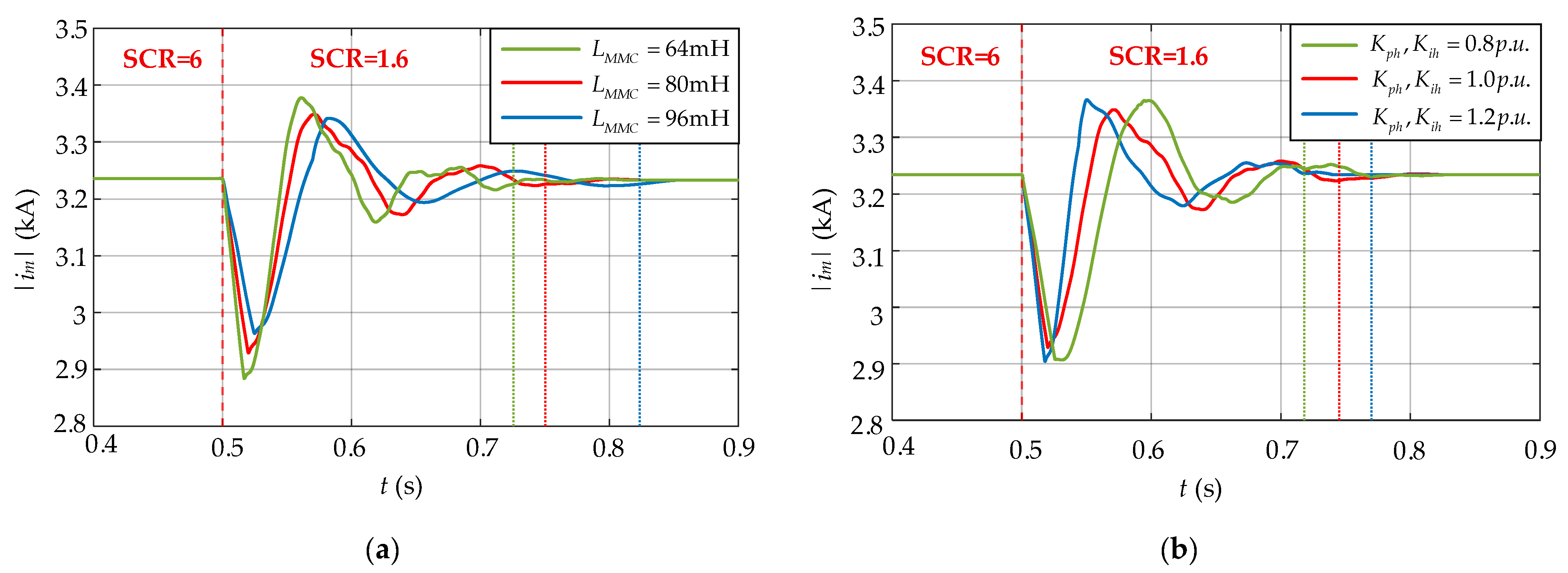
Figure 13a shows the converter current magnitude curves when the proposed method is applied and L_MMC is set to different values within ± 20% of the nominal case. The dotted lines indicate the corresponding settling times and match the curve colors. It can be observed that the transient converter current response remains well damped and eventually settles to its steady state value for all inductance values, without noticeable low frequency oscillations or any tendency toward divergence. As L_MMC increases, the current evolution becomes slower and the settling time increases, which is consistent with the practical influence of the arm inductance on the transient behavior of the current.

Figure 13b further shows the converter current magnitude under different gain scalings of the PI controller in the hybrid coefficient regulating method, where 1.0 p.u. corresponds to the nominal values of K_ph and K_ih listed in Table A1, and the remaining system parameters are kept unchanged. It can be observed that the transient current responses in all cases remain well damped and converge to the steady state value, indicating that the proposed method can maintain stable transient regulation under regulator gain deviations. When K_ph and K_ih are reduced to 0.8 p.u., the current evolution becomes slightly slower, the peak current becomes slightly higher, and the settling time becomes longer. When K_ph and K_ih are increased to 1.2 p.u., the current evolution becomes slightly faster and the settling time becomes shorter, while the peak current also becomes slightly higher. The above results indicate that the regulator gain scaling mainly affects the tradeoff between transition speed and current excursion, while the transient current suppression capability is preserved.

Table 5. Robustness evaluation of the proposed strategy under variations in L_MMC and K_ph, K_ih during SCR dives from 6 to 1.6.

	Transient Metrics	Overshoot (%)	Settling Time (ms)
System Parameters
LMMC = 80 mH; Kph,Kih = 1.0 p.u.		3.6%	245
LMMC	64 mH	4.6%	225
	96 mH	3.3%	323
Kph,Kih	0.8 p.u.	4.0%	270
	1.2 p.u.	4.1%	218

further summarizes the overshoots and settling times of the converter current magnitude for the above uncertainty cases. For the nominal case with L_MMC = 80 mH and K_ph, K_ih = 1.0 p.u., the overshoot is 3.6% and the settling time is 245 ms. When L_MMC varies to 64 mH and 96 mH, the overshoot becomes 4.6% and 3.3%, and the settling time becomes 225 ms and 323 ms, respectively. When K_ph and K_ih vary to 0.8 p.u. and 1.2 p.u. with L_MMC kept at the nominal value, the overshoot becomes 4.0% and 4.1%, and the settling time becomes 270 ms and 218 ms, respectively. The above metrics show that the proposed strategy maintains bounded current overshoot and well damped transient behavior under ± 20% deviations of both key physical parameters and regulator gains, which supports its robustness in practical weak grid applications.

6.4. Sensitivity to SCR Assessment Error and SĈR Update Delay

In the previous simulations, the estimated short-circuit ratio SĈR used as the scheduling input is assumed to be consistent with the actual SCR, while the possible assessment error and SĈR update delay with respect to SCR are not considered. In practical applications, the acquisition and update of SĈR inevitably involve assessment error and time delay. These factors may change the triggering instant and the transition process of the hybrid coefficient, thereby affecting the transient current suppression performance. Therefore, under the SCR dive from 6 to 1.6, sensitivity simulations are conducted on SCR assessment error and SĈR update delay to assess how these imperfections influence the hybrid coefficient transition and the resulting transient current response.

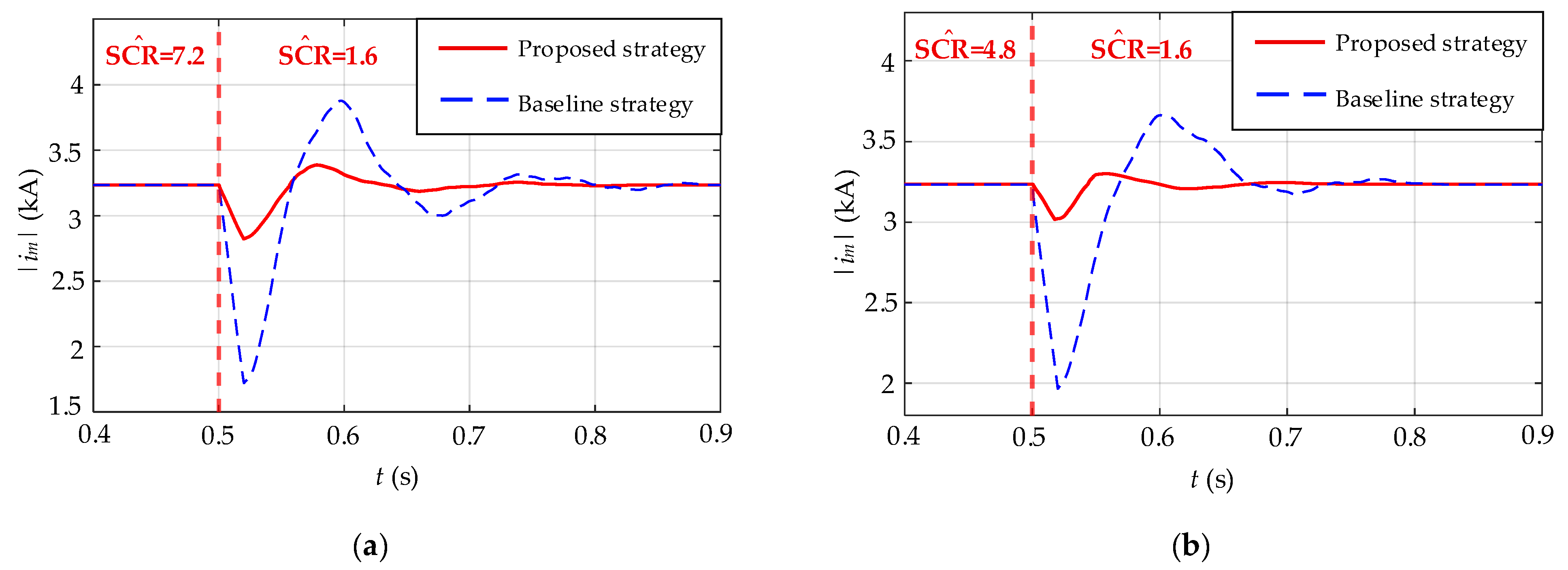
Figure 14 evaluates the sensitivity to SCR assessment error under an SCR dive from 6 to 1.6 at t = 0.5 s. Figure 14a,b correspond to +20% and −20% SCR assessment error, respectively, where the pre-event SĈR is set to 7.2 and 4.8, respectively, and SĈR is updated to 1.6 after the SCR dive. As shown in Figure 14, the proposed strategy remains effective in both cases, yielding a smoother transient current trajectory with reduced peak excursion compared with the baseline strategy. Additionally, SCR assessment error changes the pre-event value of the hybrid coefficient $k_h$ determined by SĈR, thereby altering the pre- and post-event mismatch of $k_h$, which directly affects the transient current response during the coefficient transition.

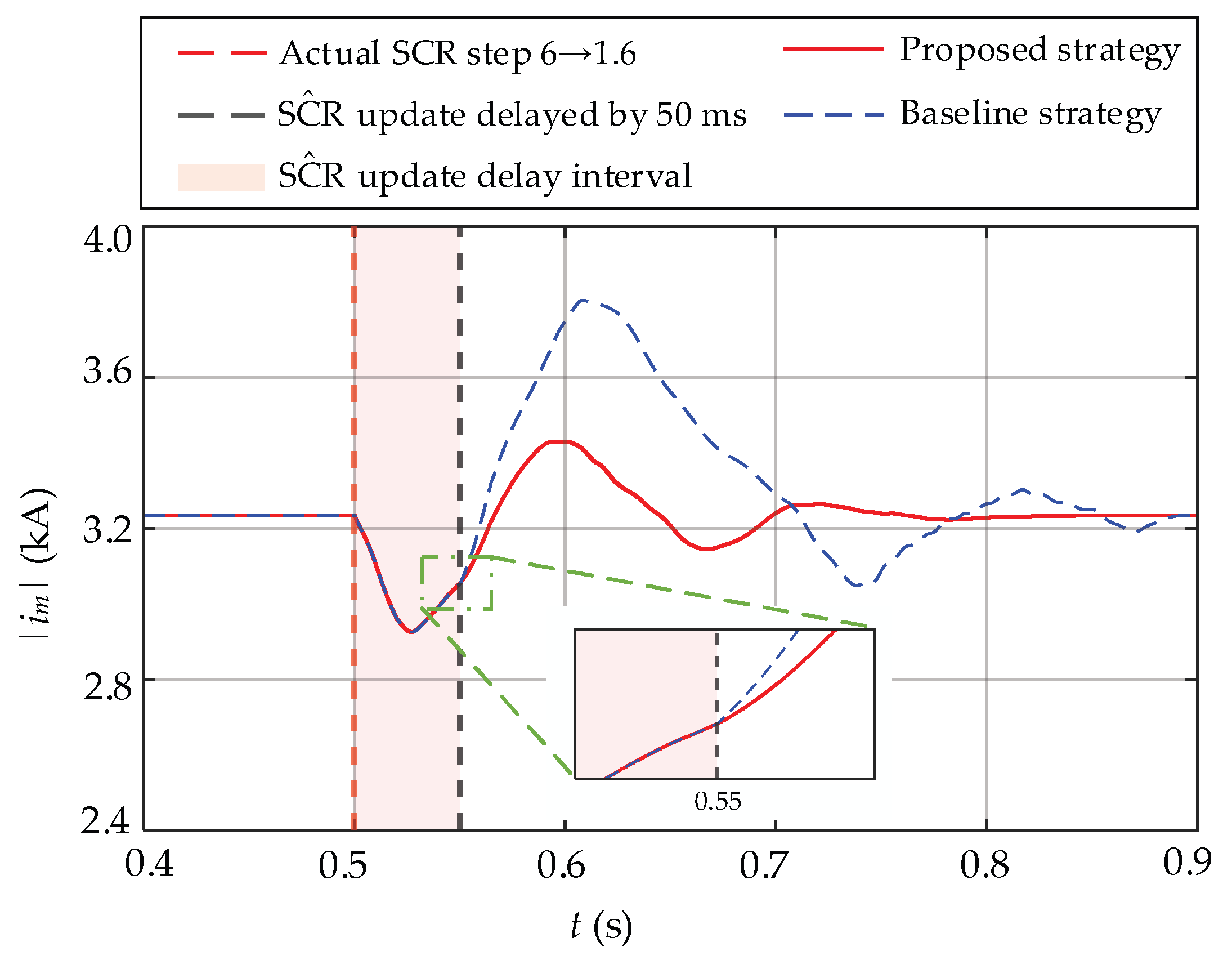
Figure 15 evaluates the sensitivity to SĈR update delay under an SCR dive from 6 to 1.6. In this test, the actual SCR changes at t = 0.5 s, while the assessed value SĈR is updated to 1.6 with a 50 ms delay. Therefore, during the interval from t = 0.5 s to t = 0.55 s, the controller still uses the pre-event SĈR = 6 and the hybrid coefficient $k_h$ remains unchanged. The transient current response in this interval is driven only by the SCR change, so the current trajectories under the baseline and proposed strategies overlap. At t = 0.55 s, SĈR is updated to 1.6 and the transient process then involves both the SCR change and the subsequent transition of $k_h$. As highlighted in the zoomed-in inset, the current slope changes noticeably after the SĈR update. The baseline strategy exhibits a faster current rise and a larger peak excursion, whereas the proposed strategy produces a smoother evolution with a reduced peak and improved damping. These results indicate that the proposed hybrid coefficient regulation effectively mitigates the transient current fluctuation when SĈR is updated with delay.

Table 6. Transient performance comparison between the baseline and proposed strategies under SCR assessment error and SĈR update delay for the SCR dive from 6 to 1.6.

Transient Metrics	Baseline Strategy		Proposed Strategy
Test Cases	Overshoot (%)	Settling Time (ms)	Overshoot (%)	Settling Time (ms)
Nominal	16.2%	351	3.6%	245
+20% SCR assessment error	19.8%	370	4.7%	305
−20% SCR assessment error	13.3%	284	2.1%	208
50 ms SĈR update delay	17.8%	387	6.0%	287

provides a quantitative comparison of transient overshoot and settling time for the SCR dive from 6 to 1.6. The nominal case corresponds to the ideal condition where SĈR is consistent with the actual SCR and is updated without assessment error or delay. The proposed strategy maintains consistently low overshoot and shorter settling time across the nominal case and all uncertainty cases, indicating reduced sensitivity to SCR assessment error and SĈR update delay. Specifically, the overshoot under the proposed strategy remains within 2.1–6.0% in all cases, whereas the baseline overshoot stays above 13.3%. The settling time is also reduced from 284 to 387 ms for the baseline strategy to 208–305 ms for the proposed strategy, confirming improved damping and faster recovery under imperfect SĈR information.

7. Conclusions

Current adaptive hybrid GFL-GFM control may cause transient current overshoots during online coefficient adjustments, which may pose a serious risk for large-scale VSC–HVDC stations and coupled grids. This issue is analyzed in this paper based on a mathematical model and the proposed adaptive hybrid GFL-GFM control with a hybrid coefficient regulating method. The main contributions of this study are as follows:

• Small-signal state–space models are established and eigenvalue analysis confirms that the proposed adaptive hybrid GFL-GFM control with a hybrid coefficient regulating method is small-signal stable over the considered SCR range. Since the regulating method is inactive in steady-state and enforces ${\dot{k}}_h=0$, the eigenvalue properties are preserved at the operating point.
• The influence mechanism of hybrid coefficient dynamics on transient current is revealed by deriving the dynamic equations of the converter current change rate within the hybrid control framework. The analysis clarifies that the hybrid coefficient change rate ${\dot{k}}_h$ exerts a significant effect as a time-varying gain and has a direct impact on the converter transient current.
• The proposed strategy exhibits good adaptability to different grid strengths. For a strong system, the hybrid coefficient can be adjusted with a higher rate of change to exploit the converter’s dynamic performance. For a weak system, a lower rate of change is adopted to suppress control-induced current transients and reduce the additional disturbance to the weak grid.
• Simulations based on a practical engineering case are carried out to validate the proposed strategy. The baseline SCR-adaptive hybrid control achieves stable operation over a wide SCR range compared with conventional GFL and GFM controls, and the proposed strategy further suppresses transient current excursions and associated power oscillations during coefficient transitions. The simulation results also verify that the method can effectively accommodate system parameter uncertainties and maintain satisfactory dynamic performance when key system parameters, such as the converter arm inductance, deviate from their nominal values within a reasonable range. Sensitivity simulations further show that the proposed strategy remains effective under representative SĈR error and update delay during SCR changes.

Nevertheless, the present study still has several limitations. The validation is restricted to simulations of a single point-to-point VSC-HVDC system, and practical aspects of real-time implementation of the proposed regulator, such as computational burden, measurement noise, discretization effects, and communication delays, have not yet been addressed. Thus, future work will focus on hardware-in-the-loop and experimental verification, as well as extensions of the method to multi-converter and multi-terminal VSC-HVDC systems operating under a wider range of grid conditions and parameter and operating condition uncertainties.

Overall, the results of the present work provide theoretical and technical references for the design and operation of similar VSC-HVDC projects.

References

- Bloom, A.; Novacheck, J.; Brinkman, G.; McCalley, J.; Figueroa-Acevedo, A.; Jahanbani-Ardakani, A.; Nosair, H.; Venkatraman, A.; Caspary, J.; Osborn, D.; et al. The Value of Increased HVDC Capacity Between Eastern and Western U.S. Grids: The Interconnections Seam Study. IEEE Trans. Power Syst. 2022, 37, 1760–1769. [Google Scholar] [CrossRef]
- Kumar, D.; Shireen, W.; Ram, N. Grid Integration of Offshore Wind Energy: A Review on Fault Ride Through Techniques for MMC-HVDC Systems. Energies 2024, 17, 5308. [Google Scholar] [CrossRef]
- Qaisar, M.W.; Fang, J. Grid-Forming Converters for Renewable Generation: A Comprehensive Review. Energies 2025, 18, 4565. [Google Scholar] [CrossRef]
- Hong, Q.T.; Khan, M.A.U.; Henderson, C.; Egea-Àlvarez, A.; Tzelepis, D.; Booth, C. Addressing Frequency Control Challenges in Future Low-Inertia Power Systems: A Great Britain Perspective. Engineering 2021, 7, 1057–1063. [Google Scholar] [CrossRef]
- Taul, M.G.; Wu, C.; Chou, S.-F.; Blaabjerg, F. Optimal Controller Design for Transient Stability Enhancement of Grid-Following Converters under Weak-Grid Conditions. IEEE Trans. Power Electron. 2021, 36, 10251–10264. [Google Scholar] [CrossRef]
- Huang, Y.; Yuan, X.; Hu, J.; Zhou, P. Modeling of VSC Connected to Weak Grid for Stability Analysis of DC-Link Voltage Control. IEEE J. Emerg. Sel. Top. Power Electron. 2015, 3, 1193–1204. [Google Scholar] [CrossRef]
- Davari, M.; Mohamed, Y.A.R.I. Robust Vector Control of a Very Weak Grid-Connected Voltage-Source Converter Considering the Phase-Locked Loop Dynamics. IEEE Trans. Power Electron. 2017, 32, 977–994. [Google Scholar] [CrossRef]
- Wang, P.; Ma, J.; Zhang, R.; Wang, S.; Liu, T.; Wu, Z.; Wang, R. Power Self-Synchronization Control of Grid-Forming Voltage-Source Converters Against a Wide Range of Short-Circuit Ratio. IEEE Trans. Power Electron. 2023, 38, 15419–15432. [Google Scholar] [CrossRef]
- Zhang, H.; Xiang, W.; Lin, W.; Wen, J. Grid-Forming Converters in Renewable Energy Sources Dominated Power Grid: Control Strategy, Stability, Application, and Challenges. J. Mod. Power Syst. Clean Energy 2021, 9, 1239–1256. [Google Scholar] [CrossRef]
- Liu, W.; Wang, R.; Kerekes, T.; Dragicevic, T.; Teodorescu, R. Capacitor Voltage Feedforward-Based Voltage Loop Control for Grid-Forming Modular Multilevel Converters Under Wide Range of Grid Strength. IEEE Trans. Power Electron. 2023, 38, 14968–14979. [Google Scholar] [CrossRef]
- Tafti, H.D.; Konstantinou, G.; Fletcher, J.E.; Callegaro, L.; Farivar, G.G.; Pou, J. Control of Distributed Photovoltaic Inverters for Frequency Support and System Recovery. IEEE Trans. Power Electron. 2022, 37, 4742–4750. [Google Scholar] [CrossRef]
- Pan, D.; Wang, X.; Liu, F.; Shi, R. Transient Stability of Voltage-Source Converters with Grid-Forming Control: A Design-Oriented Study. IEEE J. Emerg. Sel. Top. Power Electron. 2020, 8, 1019–1033. [Google Scholar] [CrossRef]
- Sang, W.; Guo, W.; Dai, S.; Tian, C.; Yu, S.; Teng, Y. Virtual Synchronous Generator, a Comprehensive Overview. Energies 2022, 15, 6148. [Google Scholar] [CrossRef]
- Almutairi, S.Z. Dynamic Interactions between Parallel Grid-Forming Inverters in a Microgrid. Appl. Sci. 2023, 13, 6989. [Google Scholar] [CrossRef]
- Hong, Z.; Xu, H.; Hou, Z.; Zhan, M. Origin of Anomalous Instability of Grid-Forming Converters Tied to Stiff Grids. IET Renew. Power Gener. 2023, 17, 2563–2574. [Google Scholar] [CrossRef]
- Gao, X.; Zhou, D.; Anvari-Moghaddam, A.; Blaabjerg, F. Grid-Following and Grid-Forming Control in Power Electronic Based Power Systems: A Comparative Study. In Proceedings of the IECON 2021—47th Annual Conference of the IEEE Industrial Electronics Society, Toronto, ON, Canada, 13–16 October 2021; pp. 1–6. [Google Scholar] [CrossRef]
- Babu, V.V.; Roselyn, J.P.; Nithya, C.; Sundaravadivel, P. Development of Grid-Forming and Grid-Following Inverter Control in Microgrid Network Ensuring Grid Stability and Frequency Response. Electronics 2024, 13, 1958. [Google Scholar] [CrossRef]
- Li, M.; Zhang, X.; Guo, Z.; Pan, H.; Ma, M.; Zhao, W. Impedance Adaptive Dual-Mode Control of Grid-Connected Inverters with Large Fluctuation of SCR and Its Stability Analysis Based on D-Partition Method. IEEE Trans. Power Electron. 2021, 36, 14420–14435. [Google Scholar] [CrossRef]
- Sun, P.; Xu, H.; Yao, J.; Chi, Y.; Huang, S.; Cao, J. Dynamic Interaction Analysis and Damping Control Strategy of Hybrid System with Grid-Forming and Grid-Following Control Modes. IEEE Trans. Energy Convers. 2023, 38, 1639–1649. [Google Scholar] [CrossRef]
- Singhal, A.; Vu, T.L.; Du, W. Consensus Control for Coordinating Grid-Forming and Grid-Following Inverters in Microgrids. IEEE Trans. Smart Grid 2022, 13, 4123–4133. [Google Scholar] [CrossRef]
- Lima, L.A.M.; Watanabe, E.H. Hybrid Control Scheme for VSC Presenting Both Grid-Forming and Grid-Following Capabilities. IEEE Trans. Power Deliv. 2022, 37, 4570–4581. [Google Scholar] [CrossRef]
- Han, F.; Zhang, X.; Li, M.; Li, F.; Zhao, W. Stability Control for Grid-Connected Inverters Based on Hybrid-Mode of Grid-Following and Grid-Forming. IEEE Trans. Ind. Electron. 2024, 71, 10750–10760. [Google Scholar] [CrossRef]
- Liu, P.; Xie, X.; Shair, J. Adaptive Hybrid Grid-Forming and Grid-Following Control of IBRs with Enhanced Small-Signal Stability Under Varying SCRs. IEEE Trans. Power Electron. 2024, 39, 6603–6607. [Google Scholar] [CrossRef]
- Chen, J.; Prystupczuk, F.; O’Donnell, T. Use of Voltage Limits for Current Limitations in Grid-Forming Converters. CSEE J. Power Energy Syst. 2020, 6, 259–269. [Google Scholar] [CrossRef]
- Baeckeland, N.; Chatterjee, D.; Lu, M.; Johnson, B.; Seo, G.-S. Overcurrent Limiting in Grid-Forming Inverters: A Comprehensive Review and Discussion. IEEE Trans. Power Electron. 2024, 39, 14493–14517. [Google Scholar] [CrossRef]
- Liu, X.; Yang, H.; Zhou, Y. Impact of Short-Circuit Ratio Change to HVDC Operating Characteristics. In Proceedings of the 2011 Asia-Pacific Power and Energy Engineering Conference, Wuhan, China, 25–28 March 2011; pp. 1–4. [Google Scholar] [CrossRef]
- Gao, X.; Zhou, D.; Anvari-Moghaddam, A.; Blaabjerg, F. Seamless Switching Method Between Grid-Following and Grid-Forming Control for Renewable Energy Conversion Systems. IEEE Trans. Ind. Appl. 2025, 61, 597–606. [Google Scholar] [CrossRef]
- Jiang, G.; Kan, S.; Li, Y.; Zhu, X. Disturbance-Free Switching Control Strategy for Grid-Following/Grid-Forming Modes of Energy Storage Converters. Electronics 2025, 14, 3963. [Google Scholar] [CrossRef]
- Nami, A.; Liang, J.; Dijkhuizen, F.; Demetriades, G.D. Modular Multilevel Converters for HVDC Applications: Review on Converter Cells and Functionalities. IEEE Trans. Power Electron. 2015, 30, 18–36. [Google Scholar] [CrossRef]
- Wu, D.; Li, G.; Javadi, M.; Malyscheff, A.M.; Hong, M.; Jiang, J.N. Assessing Impact of Renewable Energy Integration on System Strength Using Site-Dependent Short Circuit Ratio. IEEE Trans. Sustain. Energy 2018, 9, 1072–1080. [Google Scholar] [CrossRef]
- Abdelkader, S.M.; Morrow, D.J. Online Thévenin Equivalent Determination Considering System Side Changes and Measurement Errors. IEEE Trans. Power Syst. 2015, 30, 2716–2725. [Google Scholar] [CrossRef]
- Mohammed, N.; Kerekes, T.; Ciobotaru, M. An Online Event-based Grid Impedance Estimation Technique Using Grid-connected Inverters. IEEE Trans. Power Electron. 2021, 36, 6106–6117. [Google Scholar] [CrossRef]
- Nguyen, N.H.; Nguyen, P.D. Overshoot and settling time assignment with PID for first-order and second-order systems. IET Control Theory Appl. 2018, 12, 2407–2416. [Google Scholar] [CrossRef]
Figure 1.
Diagram of adaptive hybrid GFL-GFM control with hybrid-coefficient transition regulation. The superscript * denotes the reference value.
Figure 2.
Detailed block diagram of the proposed hybrid GFL-GFM control scheme. The superscript * denotes the reference value.
Figure 3.
Eigenvalue loci of the converter under GFL control with SCR reduced from 16 (initial) to 1.6 (final).
Figure 4.
Eigenvalue loci of the converter under GFM control with SCR reduced from 16 (initial) to 1.6 (final).
Figure 5.
Eigenvalue loci of the converter under proposed hybrid control with SCR reduced from 16 (initial) to 1.6 (final).
Figure 6.
Diagram of the hybrid coefficient regulating method.
Figure 7.
Active-power responses under GFL control and baseline strategy with SCR decreasing from 16 to 1.6.
Figure 8.
Active-power responses under GFM control and baseline strategy with SCR increasing from 1.6 to 16.
Figure 9.
and under the proposed strategy with SCR decreasing from 16 to 1.6.
Figure 10.
Converter responses under the baseline and proposed strategies with SCR decreasing from 16 to 1.6: (a) Current vector magnitude curves. (b) Active power curves. (c) Reactive power curves.
Figure 11.
and under the proposed strategy with SCR increasing from 1.6 to 16.
Figure 12.
Converter responses under the baseline and proposed strategies with SCR increasing from 1.6 to 16. (a) Current vector magnitude curves. (b) Active power curves. (c) Reactive power curves.
Figure 13.
Converter current magnitude of the proposed strategy under parameter variations during SCR dives from 6 to 1.6: (a) Different converter arm inductances LMMC. (b) Different gain scalings of Kph and Kih. The dotted lines indicate the corresponding settling times and match the curve colors.
Figure 14.
Converter current magnitude under the baseline and proposed strategies with ±20% SCR assessment error during the SCR dive from 6 to 1.6: (a) +20% SCR assessment error. (b) −20% SCR assessment error.
Figure 15.
Converter current magnitude under the baseline and proposed strategies with 50 ms SĈR update delay during SCR dives from 6 to 1.6.