Statistical Cost Anomaly Screening and Explanation for Preliminary Design Estimates of Power Grid Substation Projects

Abstract

Reliable review of preliminary design estimates is important for cost control in power grid substation projects, yet fixed thresholds have limited ability to reflect project-specific engineering conditions. This study develops a multidimensional cost-deviation screening framework integrating CatBoost, Conformalized Quantile Regression (CQR), Cost Structure family-wise calibration, and SHapley Additive exPlanations (SHAP)feature attribution. Total Cost, Unit Cost, and Cost Structure are evaluated jointly, with CQR providing project-specific marginal prediction intervals and an economic-exposure-weighted calibration controlling simultaneous screening across the five Cost Structure components. SHAP is subsequently used to provide feature-level interpretation of screened projects. The framework was evaluated using 906 substation projects from 27 provincial grid companies in China, including 761 projects for development and 145 for held-out evaluation. CatBoost achieved $R^2$ values of 0.9363 for Total Cost and 0.8899 for Unit Cost. After Cost Structure family-wise calibration, 22 held-out projects (15.17%) received review flags. Incorporating Cost Structure increased the number of flagged projects from 15 to 22, identifying seven additional projects not flaggedby Total Cost or Unit Cost alone. The results demonstrate competitive predictive performance and the incremental screening value of Cost Structure, although prediction-interval efficiency remained target dependent. The proposed framework provides an uncertainty-aware and interpretable approach for prioritizing preliminary-design cost review.

1. Introduction

Continued investment in power grid infrastructure has increased the need for reliable cost review of substation projects [1,2]. Preliminary design estimates are particularly important because they provide the basis for investment approval, budget control, and subsequent engineering review [3,4,5,6,7,8]. At this stage, project costs vary with voltage level, transformer capacity, equipment configuration, construction conditions, regional characteristics, and other engineering factors [9,10,11,12]. Expert rules and fixed thresholds are easy to apply but have limited ability to reflect such project heterogeneity [13]. Data-driven methods can provide project-specific cost references and support the identification of projects that require further examination [14,15,16,17,18].

Machine learning has been widely applied to construction cost prediction and related engineering applications. Existing studies have examined ensemble models for early-stage cost estimation [19], neural-network models incorporating economic and project information [20], substation cost prediction [21], and multioutput prediction of construction cost components [22]. Predictive models have also been introduced into construction cost auditing [23], while uncertainty information and SHAP have been used to improve the reliability and interpretability of cost prediction [24]. These studies demonstrate the value of point prediction, multioutput modeling, auditing-oriented applications, uncertainty assessment, and model interpretation, but these elements have largely been examined separately. For preliminary-design review of substation projects, a unified framework that integrates multidimensional cost representation, project-specific uncertainty-aware screening, multiplicity control for simultaneous Cost Structure evaluation, and post-screening feature attribution remains insufficiently developed.

For preliminary design review of substation projects, cost information can be examined from several complementary perspectives. Total Cost reflects the overall investment level, Unit Cost describes cost relative to transformer capacity, and Cost Structure represents the allocation among major cost components. Considering these dimensions together provides a broader view of project cost characteristics than using an aggregate cost measure alone. In addition, several cost targets are evaluated for each project. Their prediction intervals therefore need to be incorporated into a consistent project-level screening procedure. Model interpretation can further provide feature-level information for understanding the predictions associated with flagged projects.

Based on these considerations, this study develops a cost-deviation screening framework for preliminary design estimates of power grid substation projects. CatBoost is used to generate point predictions for Total Cost, Unit Cost, and Cost Structure. Conformalized Quantile Regression (CQR) is used to construct project-specific marginal prediction intervals for the seven underlying cost targets. To address the simultaneous use of the five Cost Structure intervals, a family-wise calibration is applied within the Cost Structure dimension, while the Total Cost and Unit Cost marginal intervals are retained unchanged. The resulting dimensional indicators are then combined to determine the final project-level review flags. SHAP feature attribution is subsequently used to characterize the contributions of recorded engineering features to the CatBoost point predictions.

The main contributions of this study are threefold. First, preliminary design estimates are evaluated through the complementary dimensions of Total Cost, Unit Cost, and Cost Structure, allowing aggregate cost, capacity-normalized cost, and internal cost allocation to be examined within one framework. Second, CQR-based uncertainty assessment is combined with Cost Structure family-wise calibration to address the simultaneous evaluation of multiple cost-share intervals before dimensional screening results are integrated at the project level. Third, the framework links project screening with SHAP feature attribution to provide feature-level information for subsequent engineering reviews. The complete framework is evaluated on a multi-regional dataset of 906 substation projects using a fixed held-out subset for final evaluation. The empirical analysis covers predictive performance, interval reliability, project-level screening, the additional information provided by Cost Structure, robustness, and representative project interpretation.

Accordingly, the empirical evaluation is guided by four working hypotheses.

Hypothesis H1. 

CatBoost will provide competitive point-prediction performance relative to benchmark models across the three cost dimensions.

Hypothesis H2. 

Grouped CQR will yield target-specific marginal prediction intervals with empirical coverage broadly consistent with the prespecified 90% level.

Hypothesis H3. 

Cost Structure family-wise calibration will reduce the multiplicity-induced inflation of simultaneous cost-share screening signals relative to marginal screening before family-wise calibration.

Hypothesis H4. 

Cost Structure will provide incremental screening information beyond Total Cost and Unit Cost.

2. Methodology

2.1. CatBoost

CatBoost is a gradient-boosted decision-tree algorithm that supports both numerical and categorical predictors [25,26,27,28]. The present dataset contains categorical engineering attributes such as region, voltage level, equipment configuration, and wiring scheme. CatBoost processes categorical variables using ordered target statistics and applies ordered boosting to reduce prediction shift and overfitting. The boosting process can be expressed as

$$F_{\mathrm{m}}\left(x\right)=F_{m-1}\left(x\right)+\eta \cdot h_m\left(x\right),m=1,2,\dots ,M,$$

(1)

where $F_{\mathrm{m}}\left(x\right)$ is the ensemble prediction after the $m$-th boosting iteration, $h_m(x)$ is the tree added at iteration $m$, $\eta$ is the learning rate, and $M$ is the total number of boosting iterations. Each iteration updates the ensemble prediction through an additional decision tree. Equation (1) summarizes the iterative boosting update used to construct the CatBoost ensemble.

In this study, CatBoostRegressor is used to generate point predictions for Total Cost, Unit Cost, and Cost Structure. Total Cost and Unit Cost are modeled using separate single output regressors. The five Cost Structure shares are modeled jointly using a multi-output CatBoost model with the MultiRMSE objective. The resulting Cost Structure point predictions are subsequently normalized to satisfy the compositional closure constraint. Target-specific feature construction, model training, hyperparameter optimization, and final parameter settings are described in Section 3.4.1, Section 3.4.2 and Section 3.4.3 and Supplementary Sections S2 and S3.

2.2. Conformalized Quantile Regression (CQR)

Breusch–Pagan diagnostics indicated substantial heteroscedasticity ($p<0.001$), motivating the use of project-specific rather than constant-width prediction intervals. Conformalized Quantile Regression (CQR) [29,30,31] combines quantile regression with conformal calibration. The lower and upper conditional quantiles can vary with the project features, allowing the prediction interval to adapt to differences in predictive uncertainty.

For a nominal marginal coverage level of $1-\alpha$, the lower and upper conditional quantiles are estimated at $\alpha /2$ and $1-\alpha /2$. In this study, CatBoost quantile models are fitted using the quantile loss

$$L_q\left(y,{\hat{q}}_q\right)=\left\{\begin{array}{cc}q\cdot \left(y-{\hat{q}}_q\right),& y\ge {\hat{q}}_q\\ \left(1-q\right)\cdot \left({\hat{q}}_q-y\right),& y<{\hat{q}}_q\end{array}\right.$$

(2)

where $y$ is the observed value, ${\hat{q}}_q$ is the estimated conditional quantile, and $q\in \left(0,1\right)$ is the quantile level. The lower and upper quantile models correspond to $q=\alpha /2$ and $q=1-\alpha /2$, respectively.

In standard split-CQR, the quantile models are fitted on a training set and calibrated using an independent calibration set $D_{cal}$. For calibration observation $i$, the nonconformity score is

$$s_i=\max \left\{{\hat{q}}_{\alpha /2}\left(x_i\right)-y_i,y_i-{\hat{q}}_{1-\alpha /2}\left(x_i\right)\right\},$$

(3)

Let ${\mathrm{n}}_{cal}$ be the number of calibration observations and let

$$s_{(1)}\le s_{(2)}\le \cdots \le s_{(n_{cal})},$$

(4)

denote the ordered nonconformity scores. The conformal correction is obtained as

$$k=⌈(n_{cal}+1)(1-\alpha )⌉\begin{array}{cc},& Q_{1-\alpha }=s_{(k)}\end{array},$$

(5)

Using the nonconformity score in Equation (3) and the conformal correction in Equation (5), the resulting prediction interval for a new project with feature vector $x$ is

$$C_{\alpha }(x)=\left[{\hat{q}}_{\alpha /2}\left(x\right)-Q_{1-\alpha },{\hat{q}}_{1-\alpha /2}\left(x\right)+Q_{1-\alpha }\right],$$

(6)

Under the exchangeability conditions of standard split conformal prediction, this interval satisfies the marginal coverage property

$$\mathrm{Pr}\left\{Y_{test}\in C_{\alpha }\left(X_{new}\right)\right\}\ge 1-\alpha ,$$

(7)

Equation (7) gives the standard split-conformal marginal coverage result under exchangeability. Because the present implementation uses company-grouped, cross-validated calibration, and aggregation rather than a single independent calibration split, exact finite-sample coverage is not claimed; interval coverage is instead evaluated empirically on the fixed held-out test set.

These equations define the standard CQR formulation used as the methodological basis for interval construction. In this study, the nominal marginal coverage level is set to 90% ($\alpha =0.10$). The prediction intervals are implemented using grouped cross-validated, fold-specific calibration, and aggregation within the development set. The complete implementation is described in Section 3.5.

2.3. SHAP-Based Prediction Attribution

SHapley Additive exPlanations (SHAP) is a feature-attribution method based on Shapley values [32,33,34,35,36]. It represents a model prediction as the sum of a baseline value and the contributions of individual input features. For a project with feature vector $x$, the CatBoost point prediction can be expressed as

$$f\left(x\right)={\varphi }_0+{\displaystyle {\sum }_{j=1}^M{\varphi }_j},$$

(8)

where $f\left(x\right)$ is the CatBoost point prediction, ${\varphi }_0$ is the SHAP baseline value, $M$ is the number of input features, and ${\varphi }_j$ is the feature contribution of feature $j$. A positive ${\varphi }_j$ increases the prediction relative to the SHAP baseline value, while a negative ${\varphi }_j$ decreases it. The magnitude of ${\varphi }_j$ indicates the contribution of the corresponding feature to the prediction for that project.

The CatBoost models in this study are analyzed using TreeExplainer. Local SHAP attribution describes the feature contributions for an individual project. Global SHAP importance is calculated from the mean absolute SHAP value across the evaluated projects:

$$I_j={\displaystyle \frac{1}{n}}{\displaystyle {\sum }_{i=1}^n\left|{\varphi }_{ij}\right|},$$

(9)

where $I_j$ is the global SHAP importance of feature $j$, $n$ is the number of evaluated projects, and ${\varphi }_{ij}$ is the contribution of feature $j$ to the point prediction for project $i$. A larger $I_j$ indicates a larger average contribution of that feature to variation in the fitted model predictions. Equation (8) gives the local additive decomposition for an individual prediction, whereas Equation (9) aggregates the absolute local contributions to obtain global feature importance.

In this study, global SHAP importance is used to summarize the features contributing most strongly to the CatBoost predictions for Total Cost, Unit Cost, and Cost Structure. Local SHAP attribution is used for representative flagged projects to examine how their recorded engineering features contribute to the corresponding point predictions. The detailed SHAP analysis procedure is presented in Section 3.6.

3. Study Data and Analytical Framework

3.1. Data Sources and Preprocessing

3.1.1. Research Samples and Data Scope

Preliminary design estimate data were collected from 27 provincial grid companies across six regions of China: North, East, Central, Northeast, Northwest, and Southwest. The source database contained 2850 substation projects reviewed between 2018 and 2024.

A common analytical cohort was constructed for Total Cost, Unit Cost, and Cost Structure. Projects were screened sequentially according to engineering eligibility, information completeness, target-data completeness, and internal consistency. Each excluded project was assigned to the first criterion it failed. The screening process is summarized in Table 1. Projects without positive current-stage incremental main-transformer capacity were excluded because Unit Cost requires a positive capacity denominator. Records with missing essential engineering descriptors or unresolved cost and quantity information were also excluded. Missing values were retained only when they could be reconstructed uniquely from recorded data. The final screening stage checked logical, accounting, and unit consistency.

Table 1. Sequential screening from the source database to the analytical cohort.

Stage	Screening Criterion	Exclusion Rule and Data Treatment	Excluded, n	Remaining, n
Source database	Preliminary design substation projects reviewed during 2018–2024	Records from 27 provincial grid companies across six regions of China	—	2850
1	Engineering and target eligibility	Exclude projects without positive current-stage incremental main-transformer capacity, including zero-increment expansion/bay projects and projects with only reserved future transformer capacity	1503	1347
2	Mandatory project information	Exclude projects missing essential engineering descriptors, including voltage level, construction type, or current-stage main-transformer information	313	1034
3	Target and quantitative data completeness	Exclude records with missing essential cost or physical-quantity data unless the missing value can be uniquely reconstructed from recorded information; no statistical or model-based imputation is used	82	952
4	Logical, accounting, and unit consistency	Exclude records with unresolved accounting contradictions, engineering-quantity inconsistencies, or ambiguous unit errors; unambiguous unit errors are corrected	46	906
Final analytical cohort	Projects satisfying all eligibility, completeness, and consistency criteria	Common cohort used for Total Cost, Unit Cost, and Cost Structure analyses	—	906

The sequential screening resulted in a final analytical cohort of 906 complete and internally consistent projects, which was used consistently across the three cost dimensions (Table 1). The final analytical cohort therefore contained 906 projects. Complete and internally consistent projects were retained across the observed cost range. The resulting cohort provides a common sample for the three cost dimensions.

The 906 projects cover 110, 220, and 500 kV voltage levels, all six geographic regions, and several construction types. Projects reviewed in 2021 formed the largest review-period group, and 110 kV substations formed the largest voltage-level group. East China and Central China accounted for the largest regional shares, while new construction and main-transformer expansion were the two main construction types. Table 2 summarizes the sample distribution.

Table 2. Distribution of major characteristics in the analytical cohort and data partitions.

Characteristic	Category	Analytical Cohort (n = 906), n (%)	Development Set (n = 761), n (%)	Held-Out Test Set (n = 145), n (%)
Review period	2018–2020	232 (25.61)	199 (26.15)	33 (22.76)
	2021	387 (42.72)	318 (41.79)	69 (47.59)
	2022–2024	287 (31.68)	244 (32.06)	43 (29.66)
Voltage level	110 kV	636 (70.20)	534 (70.17)	102 (70.34)
	220 kV	225 (24.83)	189 (24.84)	36 (24.83)
	500 kV	45 (4.97)	38 (4.99)	7 (4.83)
Region	Northeast	22 (2.43)	18 (2.37)	4 (2.76)
	East China	401 (44.26)	337 (44.28)	64 (44.14)
	Central China	254 (28.04)	214 (28.12)	40 (27.59)
	North China	93 (10.26)	78 (10.25)	15 (10.34)
	Northwest	77 (8.50)	65 (8.54)	12 (8.28)
	Southwest	59 (6.51)	49 (6.44)	10 (6.90)
Construction nature	New construction	551 (60.82)	463 (60.84)	88 (60.69)
	Main-transformer expansion	329 (36.31)	276 (36.27)	53 (36.55)
	Other	26 (2.87)	22 (2.89)	4 (2.76)

For model development and final evaluation, the analytical cohort was subsequently divided into 761 development projects and 145 fixed held-out test projects. The detailed partitioning and validation procedure is described in Section 3.4.2. The evaluation represents project-level screening within the participating company system, where historical projects from the participating companies are available for model development.

3.1.2. Feature Construction and Selection

Candidate features were constructed from information available at the preliminary design stage. The features describe four aspects of each project: engineering attributes, construction environment, physical quantities, and review time. Engineering attributes include project background, management practices, and technical characteristics. Construction environment describes site conditions and topography. Physical quantities include major equipment parameters and civil-work quantities. Review time records the year of preliminary design review.

Feature selection followed the availability and data-integrity requirements of the screening framework. Project identifiers and free-text fields were removed. Monetary variables derived from the preliminary design estimate or otherwise directly encoding the target cost information were excluded from the predictor set. In addition, variables unavailable at the preliminary design stage and variables derived from subsequent actual costs were not used. The retained features therefore consist of project information available when the preliminary design estimate is reviewed.

The resulting 73-predictor base feature framework is summarized in Table 3. These variables form the base feature set for model development. Target-specific transformations are subsequently applied for Total Cost, Unit Cost, and Cost Structure, as described in Section 3.4.1. The complete list of final base predictors and target-specific derived predictors is provided in Supplementary Section S2 (Tables S3 and S4).

Table 3. Feature framework for model development.

Feature Group	Subcategory	Feature Count	Representative Features
Engineering attributes	Project background	6	Region; affiliated company; rated voltage at the high-, medium-, and low-voltage sides; construction nature
	Management practices	4	Standard design and cost-plan adoption; 3D design application; standardized on-site cost management
	Technical characteristics	4	Modular or prefabricated construction; water-firefighting system; prefabricated cabin; smart substation
Construction environment	Environmental conditions and topography	3	Pollution grade; altitude; topography
Physical quantities	Equipment and system parameters	39	Substation type; main-transformer configuration, quantity, and capacity; outgoing circuits; circuit breakers; wiring scheme; reactors and capacitors; cable and grounding materials
	Civil works	16	Total building area; main control building area; steel support weight; foundation concrete volume; equipment foundations; cable-trench volume; access-road length
Review time	Preliminary-design review year	1	Year of preliminary design review

3.1.3. Data Preprocessing

Monetary cost data were standardized to a common 2018 costing basis before model development. The standardization was performed at the cost-element level using the detailed project cost records. Engineering quantities and consumption levels were retained, while labor, material, and adjustable machinery prices were restated using the corresponding 2018 pricing basis. Applicable fees and charges were then recalculated under the same costing framework. The standardized cost elements were subsequently used to construct the response variables defined in Section 3.1.4; these monetary cost elements were not included as model predictors. Accordingly, inter-year price-level differences were controlled through cost-element-level repricing rather than by applying a single aggregate inflation or consumer-price index to the project total.

The retained input variables were processed according to their data types. Categorical variables included region, voltage level, construction nature, substation type, and other discrete engineering attributes. Continuous numerical variables described physical scales such as transformer capacity, building area, and cable quantity. Count variables represented quantities such as outgoing circuits, circuit breakers, and reactor banks. Categorical variables were retained as categorical inputs for CatBoost, while numerical and count variables were processed as numerical inputs. The same feature definitions were used throughout model development, with target-specific feature transformations described in Section 3.4.1. CatBoost’s native treatment of categorical features is also retained in the benchmark protocol.

Several nonnegative variables and model targets showed right-skewed distributions. A log-plus-one transformation was therefore applied where specified in the modeling pipeline:

$$z^{\prime }=\log \left(z+1\right),$$

(10)

where $z$ is the original value and $z^{\prime }$ is the transformed value. This transformation was used for skewed count and ratio variables and for the corresponding transformed prediction targets. Model outputs were converted back to their original scales before performance evaluation, interval reporting, and Cost Structure closure normalization.

3.1.4. Cost Dimensions and Target Definition

The screening framework evaluates preliminary design estimates from three complementary cost dimensions: Total Cost, Unit Cost, and Cost Structure. Total Cost describes the overall investment level of a project. Unit Cost relates project cost to current-stage incremental main-transformer capacity. Cost Structure describes the allocation of total cost among the main cost components.

Seven prediction targets are defined across the three dimensions. Total Cost and Unit Cost each contain one target. Cost Structure contains five cost shares: construction, equipment procurement, installation, other costs, and basic contingency. The target definitions are summarized in Table 4.

Table 4. Cost dimensions and prediction targets.

Target	Variable	Unit	Calculation Logic
Total Cost	Total overnight capital cost	million CNY	Overnight capital cost in the preliminary design estimate
Unit Cost	Unit capacity cost	CNY/kVA	Overnight capital cost divided by current-stage incremental main-transformer capacity
Cost Structure	Construction cost share	%	Construction cost divided by overnight capital cost × 100%
	Equipment procurement cost share	%	Equipment procurement cost divided by overnight capital cost × 100%
	Installation cost share	%	Installation cost divided by overnight capital cost × 100%
	Other-cost share	%	Other costs divided by overnight capital cost × 100%
	Basic contingency share	%	Basic contingency divided by overnight capital cost × 100%

For project $i$, Unit Cost is defined as

$$U_i={\displaystyle \frac{C_i}{K_i}},$$

(11)

where $C_i$ is the overnight capital cost and $K_i$ is the current-stage incremental main-transformer capacity, expressed in compatible CNY and kVA units. A positive $K_i$ is therefore required for Unit Cost to be defined.

For Cost Structure, let $C_{ij}$ denote the cost of component $j$ for project $i$. The corresponding cost share is

$$\begin{array}{cc}{p}_{ij}={\displaystyle \frac{C_{ij}}{C_i}},& j=1,2,\cdots ,5\end{array},$$

(12)

and the five shares satisfy the closure condition

$${\displaystyle \sum _{j=1}^5{p}_{ij}=1},$$

(13)

The five cost shares are therefore treated as five related prediction targets within the Cost Structure dimension. Their point predictions are generated jointly using the multi-output CatBoost model and subsequently normalized to satisfy the closure condition. Prediction intervals are constructed for each cost share. The detailed modeling and interval procedures are presented in Section 3.4 and Section 3.5.

3.2. Cost-Screening Framework Overview

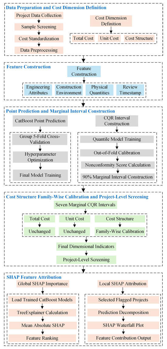
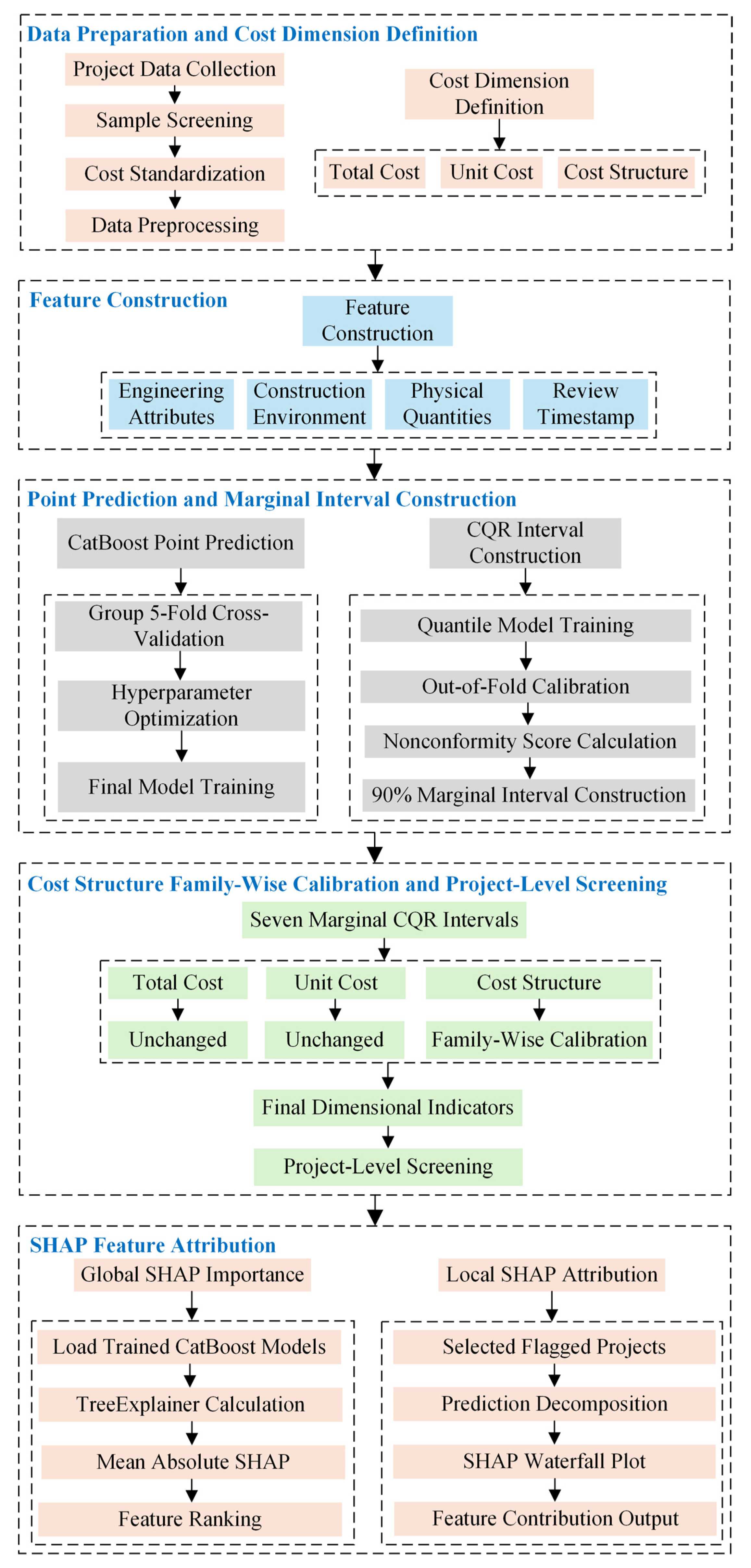
The proposed cost-screening framework follows five stages, as shown in Figure 1. The workflow integrates data preparation, point prediction, uncertainty quantification, project-level screening, and feature attribution for preliminary design estimates of power grid substation projects.

Figure 1. Cost-Screening Framework for Preliminary Design Estimates of Power Grid Substation Projects.

First, project records are filtered, standardized, and organized into three cost dimensions: Total Cost, Unit Cost, and Cost Structure. Cost Structure consists of five cost shares, resulting in seven prediction targets across the three dimensions. Input features are then constructed from engineering attributes, construction environment, physical quantities, and review timestamp.

Second, CatBoost generates point predictions for the three cost dimensions. Total Cost and Unit Cost are modeled separately, while the five Cost Structure shares are modeled jointly. CQR is then used to construct marginal prediction intervals for the seven targets. These intervals provide project-specific ranges for evaluating the observed cost values.

Third, the seven marginal CQR intervals are incorporated into the final screening procedure according to their cost dimensions. The marginal intervals for Total Cost and Unit Cost are retained unchanged. The five Cost Structure intervals are additionally processed using the economic-exposure-weighted family-wise calibration described in Section 3.5.2, producing final Cost Structure screening intervals. The resulting dimensional indicators for Total Cost, Unit Cost, and Cost Structure are then combined to determine the project-level review flag and screening category.

Finally, SHAP feature attribution is applied to the trained CatBoost point-prediction models. Global SHAP importance summarizes the contributions of input features across projects, while local SHAP attribution describes the feature contributions for representative flagged projects. Detailed procedures for data preparation, model development, interval construction, Cost Structure family-wise calibration, project-level screening, and SHAP analysis are presented in the following sections.

3.3. Statistical Screening Definitions

The screening procedure operates at two levels. Target-level violations are first identified using the seven marginal CQR intervals; the Total Cost and Unit Cost indicators are retained directly, whereas the five Cost Structure intervals undergo the family-wise calibration in Section 3.5.2 before the three-dimensional indicators are combined into the final project-level screening rule.

3.3.1. Marginal Violation Indicators

For each project, the observed values of the seven prediction targets are compared with their corresponding 90% marginal intervals. An interval violation occurs when an observed target value falls below the lower bound or above the upper bound of its marginal interval.

For project $i$ and target $j$, let $y_{ij}$ denote the observed value and $\left[L_{ij},U_{ij}\right]$ denote the corresponding marginal interval. The violation indicator is defined as

$$I_{ij}^M=\left\{\begin{array}{cc}1,& \begin{array}{ccc}{y}_{ij}<L_{ij}& or& y_{ij}>U_{ij}\end{array}\\ 0,& L_{ij}\le y_{ij}\le U_{ij}\end{array}\right.$$

(14)

where the superscript $M$ denotes evaluation using the marginal interval. Seven target-level violation indicators are obtained for each project: one for Total Cost, one for Unit Cost, and five for the Cost Structure shares.

The target-level indicators are then summarized according to the three cost dimensions. For Total Cost and Unit Cost,

$$\begin{array}{cc}{I}_{T,i}^M=I_{total,i}^M,& I_{U,i}^M=I_{unit,i}^M\end{array},$$

(15)

For Cost Structure, let $S$ denote the set of the five cost-share targets. The dimensional violation indicator is

$$I_{S,i}^M=\left\{\begin{array}{cc}1,& {\displaystyle \sum _{j\in S}{I}_{ij}^M\ge 1}\\ 0,& {\displaystyle \sum _{j\in S}{I}_{ij}^M=0}\end{array}\right.$$

(16)

where $S$ denotes the set of the five Cost Structure targets. Thus, $I_{S,i}^M=1$ when at least one of the five cost shares has an interval violation. If multiple cost shares have interval violations within the same project, these are retained as component-level results within the single Cost Structure dimension.

Table 5 summarizes the relationship between the seven target-level indicators and the three cost dimensions. These marginal violation indicators summarize the target-level screening results. The Total Cost and Unit Cost indicators are retained unchanged for final screening, whereas the five Cost Structure marginal intervals are further processed through the family-wise calibration described in Section 3.5.2.

Table 5. Summary of marginal violation indicators by cost dimension.

Cost Dimension	Prediction Target	Marginal Violation Condition	Dimensional Indicator
Total Cost	Total overnight capital cost	Observed Total Cost is outside its marginal interval	$I_{T,i}^M$
Unit Cost	Unit capacity cost	Observed Unit Cost is outside its marginal interval	$I_{U,i}^M$
Cost Structure	Five cost shares	At least one observed cost share is outside its marginal interval	$I_{S,i}^M$

3.3.2. Project-Level Screening Rules

Final project-level screening combines the unchanged marginal CQR violation indicators for Total Cost and Unit Cost with the Cost Structure violation indicator obtained after the family-wise calibration described in Section 3.5.2. For project $i$, let $I_{T,i}$, $I_{U,i}$, and $I_{S,i}$ denote the final dimensional violation indicators for Total Cost, Unit Cost, and Cost Structure, respectively. Because Total Cost and Unit Cost are not subjected to the subsequent family-wise expansion, their final dimensional indicators are identical to their marginal dimensional indicators:

$$\begin{array}{cc}{I}_{T,i}=I_{T,i}^M,& I_{U,i}=I_{U,i}^M\end{array},$$

(17)

For Cost Structure, the five marginal intervals are processed using the economic-exposure-weighted family-wise calibration described in Section 3.5.2. The raw family-wise-expanded intervals are subsequently intersected with the known feasible range $\left[0,1\right]$ of cost shares. The resulting support-constrained intervals are referred to as the final Cost Structure screening intervals. The Cost Structure dimension is activated when at least one of the five observed cost shares lies outside its corresponding final screening interval. Thus, $I_{S,i}=1$ when any Cost Structure target has a final interval violation and $I_{S,i}=0$ otherwise.

The number of cost dimensions with final interval violations is defined as

$$D_i=I_{T,i}+I_{U,i}+I_{S,i}.$$

(18)

According to Equation (18), a project is unflagged when $D_i=0$ and receives a review flag when $D_i\ge 1$. If only one dimension is activated, the project is assigned to the corresponding single-dimension category: Total-cost flag, Unit-cost flag, or Cost-structure flag. If two or all three dimensions are activated, the project is assigned to the Multi-dimension flag category. The resulting classification rules are summarized in Table 6.

Table 6. Project-level screening rules based on adjusted dimensional violation indicators.

Screening Result	Indicator Pattern (${\mathit{I}}_{\mathit{T},\mathit{i}}$, ${\mathit{I}}_{\mathit{U},\mathit{i}}$, ${\mathit{I}}_{\mathit{S},\mathit{i}}$)	Definition
Unflagged	$(0,0,0)$	No final dimensional interval violation
Total-cost flag	$(1,0,0)$	Marginal CQR interval violation in Total Cost only
Unit-cost flag	$(0,1,0)$	Marginal CQR interval violation in Unit Cost only
Cost-structure flag	$(0,0,1)$	At least one Cost Structure share violates its final family-wise-calibrated screening interval, with no Total Cost or Unit Cost violation
Multi-dimension flag	$(1,1,0)$$, (1,0,1)$, $(0,1,1)$ or $(1,1,1)$	Final dimensional violations in two or three cost dimensions

The rules cover all eight possible combinations of the three binary dimensional indicators. Each project is therefore assigned to one screening result. For projects with a Cost-structure flag or a Multi-dimension flag involving Cost Structure, the specific cost shares with adjusted interval violations are retained as component-level screening results.

3.4. Predictive Model Development

3.4.1. Target-Specific Feature Engineering

The base feature set defined in Section 3.1.2 was further processed to construct target-specific model inputs. The transformations were based on the engineering meaning and scale of the corresponding prediction targets.

For equipment described by both quantity and unit capacity, total-capacity features were calculated as the product of these two variables. This transformation was applied to reactive-power equipment, including high-voltage reactors, low-voltage capacitors, and low-voltage reactors. The resulting variables represent the installed scale of the corresponding equipment.

For Unit Cost, selected physical-quantity features were normalized by engineering scale. Transformer-related quantities were divided by the current-stage incremental main-transformer capacity, while circuit-related quantities were divided by the corresponding outgoing-circuit counts. This procedure generated 22 additional scale-normalized predictors, including circuit-breaker quantities, reactive-power equipment capacities, cable quantities, building areas, structural steel weights, and foundation-concrete volumes. The complete set of Unit Cost-specific scale-normalized predictors and their corresponding normalization bases and model treatments is reported in Supplementary Table S4.

High-cardinality categorical variables, including detailed equipment models and wiring configurations, were grouped into generalized engineering representations before model fitting. The resulting target-specific feature sets were then used consistently in CatBoost model development and the corresponding benchmark models.

3.4.2. Data Partitioning and Validation

The 906-project analytical cohort was divided into a development set of 761 projects and a fixed held-out test set of 145 projects. The partition was performed at the project level with stratification by affiliated provincial grid company, so that participating companies were represented in both subsets where sample size permitted (Table 2).

All model development was conducted using the development set. Model selection and hyperparameter optimization used five-fold GroupKFold cross-validation with affiliated provincial grid company as the grouping variable, ensuring that projects from the same company were assigned to the same fold. After hyperparameter selection, the final point-prediction models were fitted using the full development set. CQR calibration and the subsequent Cost Structure family-wise calibration were also performed exclusively using development data. The fixed held-out test set was used only for final evaluation of point-prediction performance, prediction-interval performance, and project-level screening results.

3.4.3. CatBoost Training and Hyperparameter Optimization

CatBoost point-prediction models were developed separately for the three cost dimensions using the target-specific feature sets described in Section 3.4.1. Total Cost and Unit Cost were modeled using separate single-output CatBoost regressors, whereas the five Cost Structure shares were modeled jointly using a five-output CatBoost regressor with the MultiRMSE objective.

Hyperparameters were optimized within the development set using two rounds of Optuna-TPE search with five-fold company-grouped cross-validation. Candidate configurations were evaluated using validation RMSE for Total Cost and Unit Cost and macro-RMSE across the five cost-share targets for Cost Structure, with validation-based early stopping. The better-performing configuration across the two rounds was retained for each cost dimension, after which the final models were fitted using the full development set. Detailed search spaces, optimization settings, and selected configurations are provided in Supplementary Section S3 (Tables S5–S7).

For Cost Structure, the five model outputs were first inverse-transformed to the original proportion scale and then closure-normalized. Let ${\tilde{p}}_{ij}$ denote the inverse-transformed point prediction for cost share $j$ of project $i$. The final Cost Structure point prediction was defined as

$${\hat{p}}_{ij}={\displaystyle \frac{\max (0,{\tilde{p}}_{ij})}{{\displaystyle \sum _{k=1}^5\max }(0,{\tilde{p}}_{ik})}},\hspace{1em}\hspace{0.33em}\hspace{0.33em}\hspace{0.33em}j=1,2,\dots ,5.$$

(19)

The resulting predictions are nonnegative and sum to one for each project. Point-prediction performance for the five Cost Structure targets was evaluated using these closure-normalized predictions. This closure normalization was applied only to the Cost Structure point predictions; the target-specific CQR intervals remained marginal intervals and were not jointly normalized.

3.4.4. Benchmark Models and Performance Evaluation

The point-prediction performance of CatBoost was compared with three benchmark models: Elastic Net, Random Forest, and XGBoost. Elastic Net provides a regularized linear benchmark, Random Forest represents a bagging-based tree ensemble, and XGBoost provides an alternative gradient-boosting model.

All benchmark models used the same development and held-out test partitions, target definitions, target-specific feature sets, and target transformations as the CatBoost models. Hyperparameter selection was conducted within the development set using the same five-fold company-grouped cross-validation framework described in Section 3.4.2, with validation RMSE used for model selection. The hyperparameter search spaces and selected target-specific configurations are reported in Supplementary Table S8.

For the benchmark models, Total Cost, Unit Cost, and each of the five Cost Structure shares were fitted using target-specific single-output models. Categorical variables were converted using one-hot encoding for algorithms without native categorical-feature processing. CatBoost retained its native handling of categorical variables. Numerical preprocessing and target transformations were kept consistent across models.

For Cost Structure, the five benchmark point predictions were inverse-transformed to the original proportion scale and processed using the same nonnegative closure-normalization procedure described in Section 3.4.3. The resulting five predicted cost shares therefore summed to one for each project before performance evaluation.

Point-prediction performance was evaluated using the coefficient of determination ($R^2$), root mean squared error (RMSE), mean absolute error (MAE), and mean absolute percentage error (MAPE). All metrics were calculated on the original target scale after inverse transformation. For Cost Structure, metrics were first calculated separately for the five cost-share targets and then summarized using their unweighted macro-average. RMSE and MAE for Cost Structure are reported in percentage points. The benchmark results are presented in Section 4.

3.5. Prediction-Interval Construction and Cost Structure Family-Wise Calibration

3.5.1. Cross-Validated CQR Calibration and Prediction-Interval Construction

The CQR formulation introduced in Section 2.2 was implemented separately for the seven prediction targets using company-grouped cross-validated calibration within the 761-project development set. A nominal marginal coverage level of 90% was prespecified, corresponding to $\alpha =0.10$ and lower and upper quantile levels of 0.05 and 0.95, respectively. The fixed 145-project held-out test set was reserved for final interval evaluation.

The development set was divided into five outer folds using GroupKFold with affiliated provincial grid company as the grouping variable. Within each outer-training portion, projects were further divided by company into model-fitting and calibration subsets, with approximately 20% assigned to calibration. Lower- and upper-quantile CatBoost models were fitted on the model-fitting subset, and the fold-specific calibration correction $Q_k$ was obtained from the empirical 90th percentile of the corresponding CQR nonconformity scores. For each held-out project, the lower- and upper-quantile predictions were averaged separately across the five outer folds, and the five-fold-specific calibration corrections were also averaged. Let $q_{0.05}\left(X\right)$ and $q_{0.95}\left(X\right)$ denote the resulting averaged lower- and upper-quantile predictions and $Q^{*}$ the averaged calibration correction. The final 90% marginal interval was

$$\left[L(X),U(X)\right]=\left[\begin{array}{cc}{\overline{q}}_{0.05}(X)-Q^{*},& {\overline{q}}_{0.95}(X)+Q^{*}\end{array}\right],$$

(20)

For descriptive reporting, the CQR midpoint was defined as $\left[q_{0.05}\left(X\right)+q_{0.95}\left(X\right)\right]/2$. It was used only as the center of the reported interval; the CatBoost point prediction remained the model output used for point-prediction evaluation and SHAP feature attribution. The resulting intervals constituted the seven marginal intervals used for target-level screening. The Total Cost and Unit Cost intervals were retained unchanged, whereas the five Cost Structure intervals were subsequently processed by the family-wise calibration described in Section 3.5.2. The complete fold-specific fitting, calibration, and aggregation procedure is provided in Supplementary Section S5.1 and Algorithm S2.

3.5.2. Cost Structure Family-Wise Calibration

The five marginal Cost Structure intervals were subsequently calibrated as a family to account for their simultaneous use in Cost Structure screening. This additional calibration was applied only to the Cost Structure dimension; the marginal CQR intervals for Total Cost and Unit Cost were retained unchanged. A family-wise miscoverage budget of ${\alpha }_S=0.10$ was prespecified. The five Cost Structure targets were organized into four calibration blocks,

$$\mathcal{B}=\{CE,I,O,B\},$$

(21)

where $CE$ contains Construction and Equipment Procurement jointly, $I$ denotes Installation, $O$ denotes Other Costs, and $B$ denotes Basic Contingency.

Calibration was performed using the 761 development projects only. For development project $i$ and Cost Structure target $j$, let $y_{ij}$ denote the observed cost share and $\left[L_{ij},U_{ij}\right]$ its OOF marginal CQR interval, with width $W_{ij}=U_{ij}-L_{ij}$. The normalized interval-exceedance score was defined as

$$r_{ij}=\left\{\begin{array}{ll}{\displaystyle \frac{L_{ij}-y_{ij}}{W_{ij}}},\hfill & y_{ij}<L_{ij},\hfill \\ 0,\hfill & L_{ij}\le y_{ij}\le U_{ij},\hfill \\ {\displaystyle \frac{y_{ij}-U_{ij}}{W_{ij}}},\hfill & y_{ij}>U_{ij}.\hfill \end{array}\right.$$

(22)

Thus, $r_{ij}=0$ when the observed cost share lies within its marginal interval, whereas $r_{ij}>0$ measures the exceedance relative to the target-specific interval width. For block $b\in \mathcal{B}$, the development-data mean economic exposure was denoted by ${\overline{p}}_b$, with $p_{i,CE}=p_{i,C}+p_{i,E}$. The normalized block weight was

$$w_b={\displaystyle \frac{{\overline{p}}_b}{{\displaystyle \sum _{b^{\prime }\in \mathcal{B}}{\overline{p}}_{b^{\prime }}}}},$$

(23)

and the family-wise miscoverage budget was allocated proportionally as

$${\alpha }_b={\alpha }_S{w}_b,\hspace{1em}\hspace{0.33em}\hspace{0.33em}\hspace{0.33em}{\displaystyle \sum _{b\in \mathcal{B}}{\alpha }_b}={\alpha }_S=0.10.$$

(24)

Let $E_b$ denote a coverage violation for block $b$. The allocation follows a weighted Bonferroni/union-bound rationale:

$$P \left({\displaystyle \underset{b\in \mathcal{B}}{\cup }{E}_b}\right)\le {\displaystyle \sum _{b\in \mathcal{B}}P}(E_b)\le {\displaystyle \sum _{b\in \mathcal{B}}{\alpha }_b}={\alpha }_S.$$

(25)

This construction defines a 90% family-wise coverage target for the Cost Structure dimension under the grouped OOF calibration scheme; it does not define the overall project-level review-flag rate.

Construction and Equipment Procurement were calibrated jointly using the block-level score

$$M_{i,b}=\left\{\begin{array}{ll}\max (r_{i,C},r_{i,E}),\hfill & b=CE,\hfill \\ r_{i,I},\hfill & b=I,\hfill \\ r_{i,O},\hfill & b=O,\hfill \\ r_{i,B},\hfill & b=B.\hfill \end{array}\right.$$

(26)

For each block $b$, the finite-sample rank and corresponding conformal correction were defined as

$$\begin{array}{c}{h}_b=\min \left\{⌈(n+1)(1-{\alpha }_b)⌉,n\right\},\\ Q_b=M_{(h_b),b},\end{array}$$

(27)

where $M_{\left(h_b\right),b}$ denotes the $h_b$-th ordered block score. For target $j$ belonging to block $b$, the marginal CQR interval was expanded as

$$\begin{array}{cc}{\tilde{L}}_{ij}^F=L_{ij}-Q_b{W}_{ij},& {\tilde{U}}_{ij}^F=U_{ij}+Q_b{W}_{ij}.\end{array}$$

(28)

Because each Cost Structure target is a proportion, the raw expanded interval was intersected with the feasible support $\left[0,1\right]$:

$$\begin{array}{cc}{L}_{ij}^F=\max \left(0,{\tilde{L}}_{ij}^F\right),& U_{ij}^F=\min \left(1,{\tilde{U}}_{ij}^F\right)\end{array}.$$

(29)

All Cost Structure calibration quantities were estimated exclusively from the development data. The resulting block-specific weights, miscoverage allocations, finite-sample ranks, conformal corrections, and interval-expansion diagnostics are reported in Supplementary Section S5.2 (Tables S9 and S10).

3.6. SHAP Feature Attribution

SHAP attribution was applied after the interval-based screening procedure. Total Cost and Unit Cost were interpreted using their final single-output CatBoost models, whereas Cost Structure used target-specific single-output attribution proxies because the primary Cost Structure predictor is a five-output MultiRMSE model followed by closure normalization. The proxies were used only for attribution, and their predictive agreement with the corresponding primary-model outputs was evaluated on the held-out set using correlation and prediction-difference metrics. SHAP therefore characterizes contributions to fitted model outputs rather than causal effects on observed cost deviations.

3.6.1. Global SHAP Importance

Global SHAP importance was calculated as the mean absolute SHAP contribution defined in Equation (9). For Total Cost and Unit Cost, the analysis was based on the corresponding final single-output CatBoost point-prediction models. For Cost Structure, global importance was calculated separately for the five target-specific attribution proxy models. Features were ranked in descending order of mean absolute SHAP value, with larger values indicating greater average contribution magnitude to the corresponding fitted model output.

3.6.2. Local SHAP Attribution

Local SHAP attribution was applied to representative screening cases. For Total Cost and Unit Cost, attribution was based on the corresponding final single-output CatBoost point-prediction models, whereas Cost Structure attribution used the relevant target-specific proxy models.

Local attribution followed the additive decomposition defined in Equation (8). Because the attributed targets were modeled on log-plus-one-transformed scales, contribution signs and relative magnitudes were interpreted on the transformed model-output scale rather than directly as changes in million CNY, CNY/kVA, or percentage points. For Cost Structure, the attributed output corresponds to the relevant target-specific proxy model rather than the final closure-normalized five-output prediction. Features were ranked by absolute local SHAP magnitude, with the sign retained to indicate contribution direction.

3.7. Robustness and Sensitivity Analyses

Several robustness and sensitivity analyses were conducted to assess the stability of the primary findings. The final CatBoost models were refitted across 20 random seeds with the data partition, feature sets, preprocessing procedures, target transformations, and selected hyperparameters held fixed. Held-out point-prediction performance was also evaluated across voltage-level and review-period subgroups without subgroup-specific retraining, while the sensitivity of percentage-based error measures to small observed values was examined using target-value diagnostics and WAPE for the five Cost Structure targets. Finally, the robustness of the development-data-derived economic-exposure weights used for Cost Structure family-wise calibration was assessed using provincial-company cluster bootstrap resampling and alternative monetary-exposure definitions. Detailed procedures and calculation formulas are provided in Supplementary Section S6.

4. Results

The proposed cost-screening framework was evaluated on the fixed held-out test set of 145 projects. The main-text results are presented in four parts: (1) point-prediction and marginal CQR interval performance for Total Cost, Unit Cost, and Cost Structure; (2) benchmark comparisons for point prediction and prediction intervals; (3) project-level screening results, including the contribution of Cost Structure; and (4) SHAP feature attribution for a representative screening case. Additional robustness and sensitivity analyses are reported in Supplementary Section S6.

4.1. Total Cost Point-Prediction and Interval Results

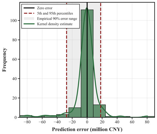
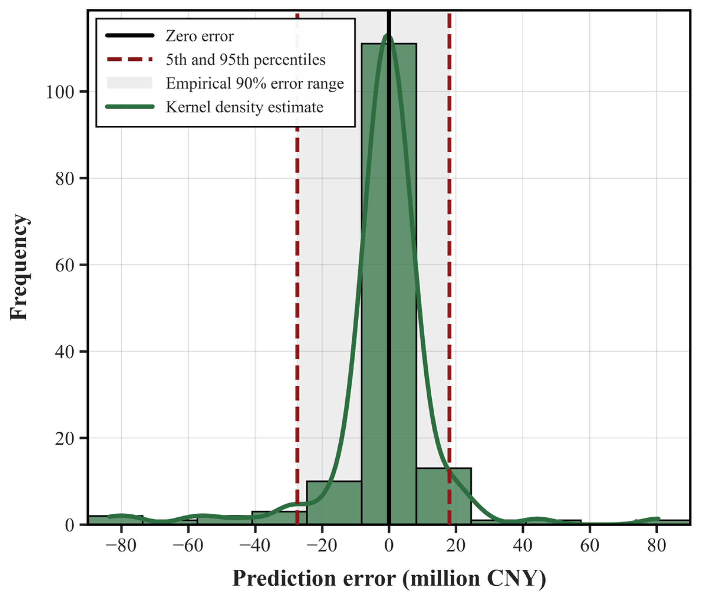
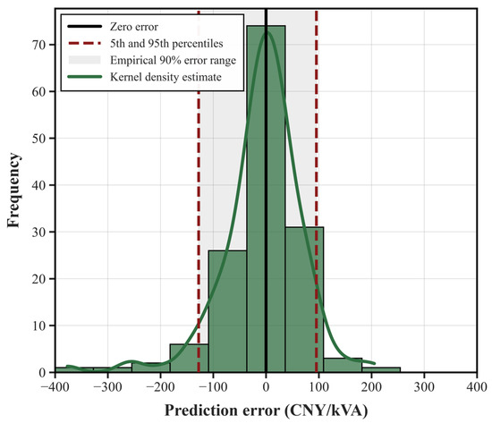
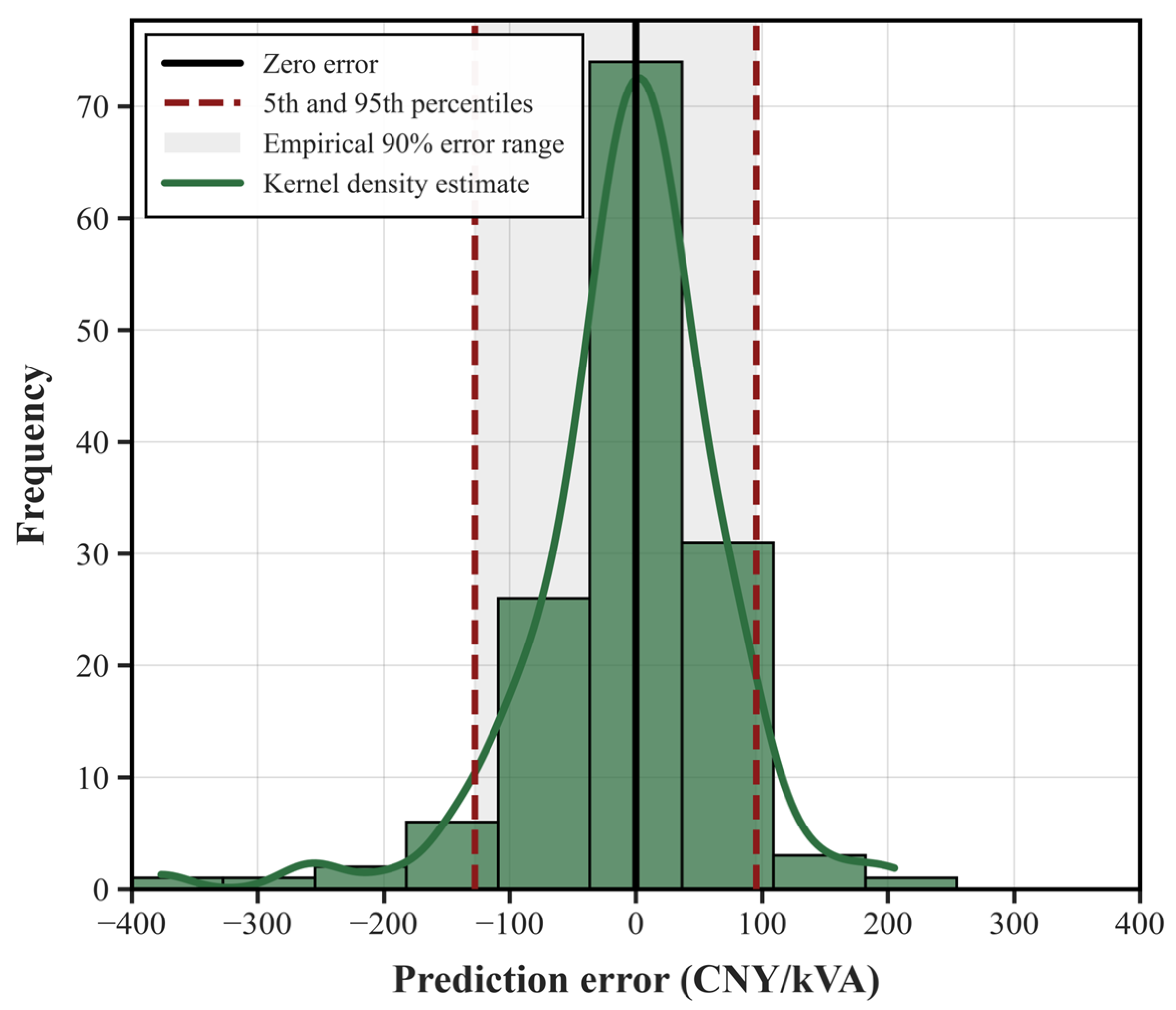
Total Cost represents the total overnight capital cost of a substation project. On the fixed held-out test set, the CatBoost point-prediction model achieved an $R^2$ of 0.9363, an RMSE of CNY 16.52 million, an MAE of CNY 8.67 million, and an MAPE of 15.34% (Table 7). Figure 2 shows the corresponding prediction-error distribution. These results indicate that the model captured a large proportion of the observed variation in Total Cost across the held-out projects.

Table 7. Point-prediction performance for Total Cost on the held-out test set.

${\mathit{R}}^2$	RMSE (Million CNY)	MAE (Million CNY)	MAPE (%)
0.9363	16.52	8.67	15.34

Figure 2. Distribution of Total Cost prediction errors on the held-out test set.

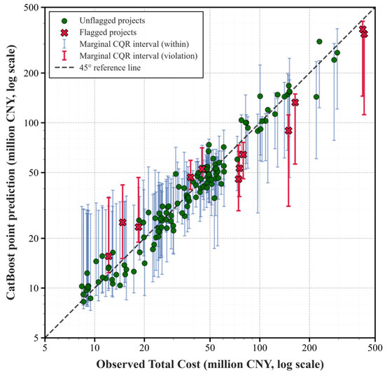
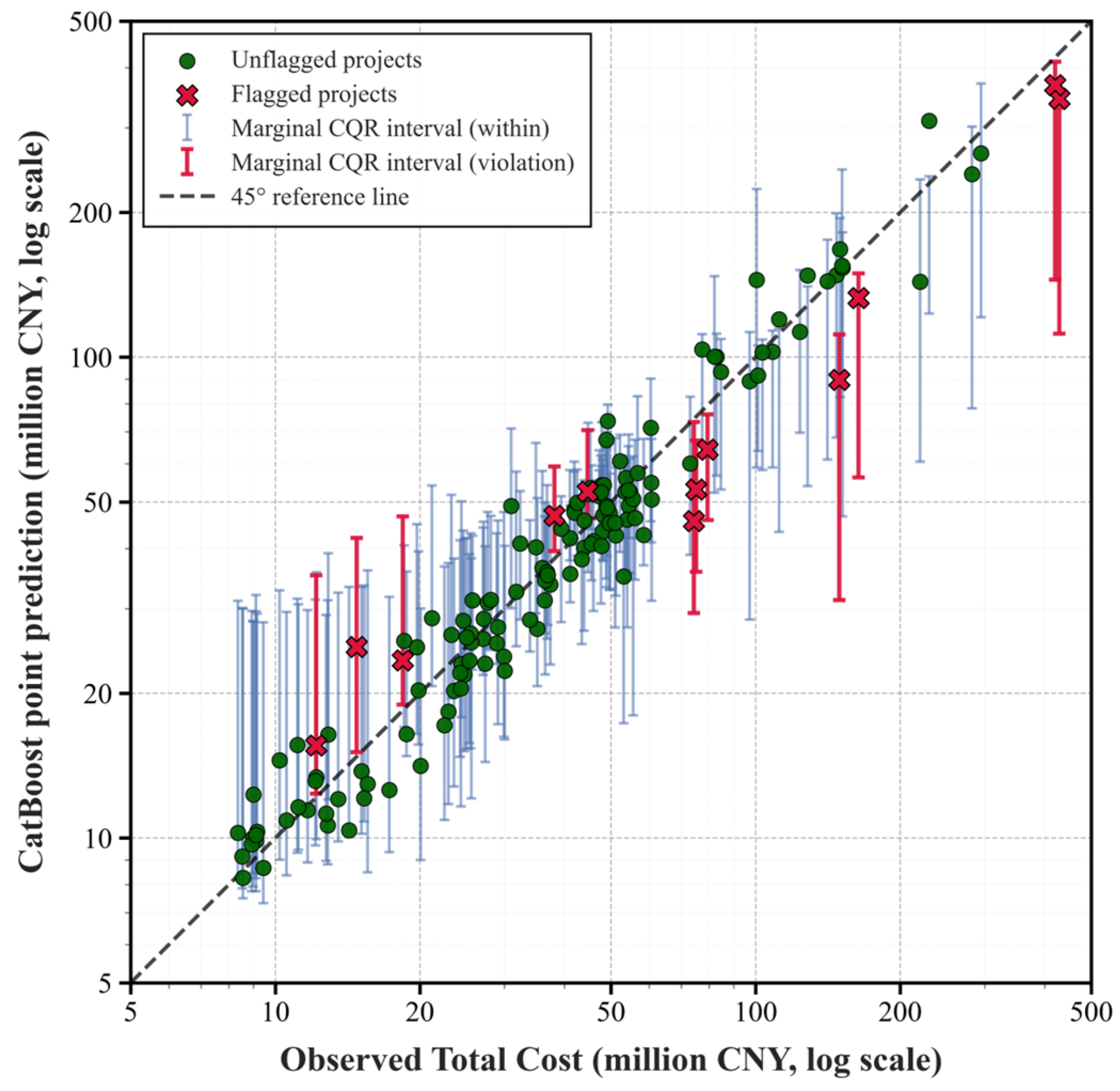
Using the cross-validated CQR procedure described in Section 3.5.1, 90% marginal intervals were constructed for the held-out projects. The empirical coverage was 91.72%, corresponding to a 1.72 percentage-point difference from the nominal 90% level, and the mean interval width was CNY 42.23 million (Table 8). Figure 3 shows the resulting project-specific marginal intervals.

Table 8. Empirical performance of the 90% marginal CQR interval for Total Cost on the held-out test set.

Nominal Coverage (%)	Empirical Coverage (%)	Mean Interval Width (Million CNY)
90.00	91.72	42.23

Figure 3. Marginal CQR intervals for Total Cost on the held-out test set.

4.2. Unit Cost Point-Prediction and Interval Results

Unit Cost relates the overnight capital cost of a project to its current-stage incremental main-transformer capacity. On the fixed held-out test set, the CatBoost point-prediction model achieved an $R^2$ of 0.8899, an RMSE of 76.01 CNY/kVA, an MAE of 52.51 CNY/kVA, and a MAPE of 16.22% (Table 9). Figure 4 shows the corresponding prediction-error distribution. These results indicate that the model captured a large proportion of the observed variation in Unit Cost across the held-out projects.

Table 9. Point-prediction performance for Unit Cost on the held-out test set.

${\mathit{R}}^2$	RMSE (CNY/kVA)	MAE (CNY/kVA)	MAPE (%)
0.8899	76.01	52.51	16.22

Figure 4. Distribution of Unit Cost prediction errors on the held-out test set.

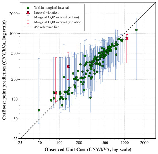
Using the cross-validated CQR procedure described in Section 3.5.1, 90% marginal intervals were constructed for the held-out projects. The empirical coverage was 97.93%, exceeding the nominal 90% level by 7.93 percentage points, and the mean interval width was 427.52 CNY/kVA (Table 10). Figure 5 shows the resulting project-specific marginal intervals.

Table 10. Empirical performance of the 90% marginal CQR interval for Unit Cost on the held-out test set.

Nominal Coverage (%)	Empirical Coverage (%)	Mean Interval Width (CNY/kVA)
90.00	97.93	427.52

Figure 5. Marginal CQR intervals for Unit Cost on the held-out test set.

4.3. Cost Structure Point-Prediction and Interval Results

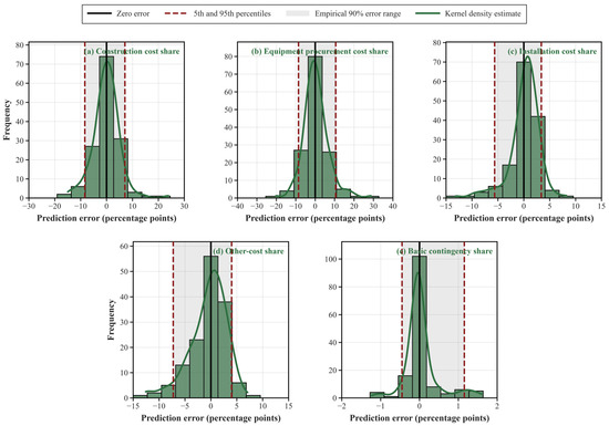
Cost Structure describes the allocation of overnight capital cost among five cost shares: construction, equipment procurement, installation, other costs, and basic contingency. The five targets were jointly predicted using the multi-output CatBoost model described in Section 3.4.3. Point-prediction performance was evaluated after inverse transformation and closure normalization. On the fixed held-out test set, the macro-average RMSE and MAE were 3.70 and 2.63 percentage points, respectively (Table 11). Among the five cost shares, basic contingency had the lowest prediction errors, with an RMSE of 0.43 percentage points and an MAE of 0.24 percentage points, while equipment procurement had the highest, with an RMSE of 6.44 percentage points and an MAE of 4.59 percentage points. Figure 6 shows the corresponding prediction-error distributions. After inverse transformation and closure normalization, the five predicted cost shares summed to 100% for each held-out project.

Table 11. Point-prediction performance for Cost Structure on the held-out test set.

Cost-Share Target	RMSE (pp)	MAE (pp)	WAPE (%)
Construction cost share	5.12	3.68	16.46
Equipment procurement cost share	6.44	4.59	9.72
Installation cost share	2.90	2.00	14.39
Other-cost share	3.60	2.65	17.46
Basic contingency share	0.43	0.24	17.02
Macro average	3.70	2.63	15.01

Figure 6. Distribution of Cost Structure prediction errors on the held-out test set.

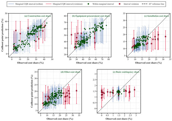
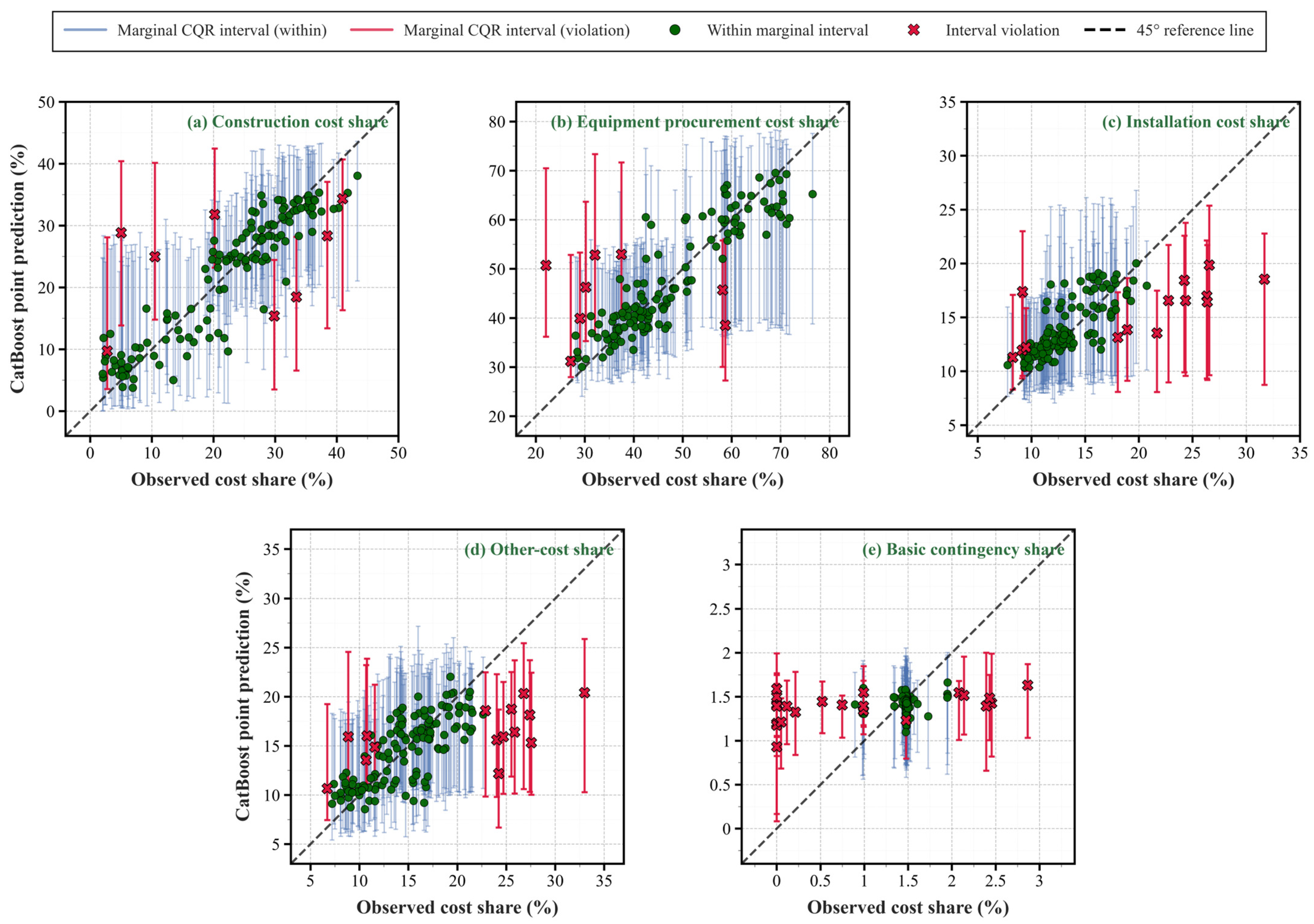
Using the cross-validated CQR procedure described in Section 3.5.1, 90% marginal intervals were constructed separately for the five cost-share targets. Empirical coverage ranged from 84.83% for basic contingency to 94.48% for construction and equipment procurement, while mean interval width ranged from 0.86 percentage points for basic contingency to 27.31 percentage points for equipment procurement (Table 12). The macro-average empirical coverage across the five targets was 90.76%, close to the nominal 90% level. Figure 7 shows the resulting marginal intervals for the five cost shares. These marginal intervals subsequently served as the inputs to the Cost Structure family-wise calibration described in Section 3.5.2, with the corresponding screening results reported in Section 4.5.

Table 12. Empirical performance of the 90% marginal CQR intervals for Cost Structure on the held-out test set.

Cost-Share Target	Empirical Coverage (%)	Mean Interval Width (pp)
Construction cost share	94.48	21.14
Equipment procurement cost share	94.48	27.31
Installation cost share	90.34	10.25
Other-cost share	89.66	12.26
Basic contingency share	84.83	0.86
Macro-average	90.76	14.36

Figure 7. Marginal CQR intervals for the five Cost Structure targets on the held-out test set.

4.4. Benchmark Comparisons

4.4.1. Point-Prediction Benchmark

Using the evaluation protocol described in Section 3.4.4, CatBoost was compared with Elastic Net, Random Forest, and XGBoost on the fixed held-out test set of 145 projects. The comparison covered Total Cost, Unit Cost, and Cost Structure. For Cost Structure, the five cost-share predictions from each benchmark method were evaluated after the same inverse transformation and closure normalization used in the primary analysis. Table 13 summarizes the held-out point-prediction results.

Table 13. Point-prediction benchmark performance on the held-out test set.

Panel A. Total Cost
Model	$R^2$	RMSE (million CNY)	MAE (million CNY)	MAPE (%)
Elastic Net	0.9181	18.74	9.32	16.53
Random Forest	0.8902	21.71	9.70	16.69
XGBoost	0.9167	18.90	9.02	15.08
CatBoost	0.9363	16.52	8.67	15.34
Panel B. Unit Cost
Model	$R^2$	RMSE (CNY/kVA)	MAE (CNY/kVA)	MAPE (%)
Elastic Net	0.8856	77.47	53.72	16.19
Random Forest	0.8059	100.94	57.70	16.34
XGBoost	0.7897	105.05	54.72	15.28
CatBoost	0.8899	76.01	52.51	16.22
Panel C. Cost Structure
Model		Macro-RMSE (pp)	Macro-MAE (pp)	Macro-WAPE (%)
Elastic Net		4.11	2.94	16.25
Random Forest		3.83	2.64	14.87
XGBoost		3.87	2.73	15.39
CatBoost		3.70	2.63	15.01

The benchmark results show that the best individual metric varied across models and cost dimensions. For Total Cost, CatBoost achieved the highest $R^2$ and the lowest RMSE and MAE, while XGBoost achieved the lowest MAPE. For Unit Cost, CatBoost likewise achieved the highest $R^2$ and the lowest RMSE and MAE, while XGBoost achieved the lowest MAPE. For Cost Structure, CatBoost achieved the lowest macro-average RMSE and MAE, while Random Forest achieved the lowest macro-average WAPE. Overall, CatBoost showed consistently competitive point-prediction performance across the three cost dimensions. These results support its use for point prediction in the subsequent CQR interval construction and cost-deviation screening analyses.

4.4.2. Prediction-Interval Benchmark

The 90% marginal CQR intervals were compared with constant-width split-conformal intervals for Total Cost, Unit Cost, and Cost Structure. Both methods were evaluated on the fixed held-out test set of 145 projects at the same nominal marginal coverage level of 90%. The comparison was conducted at the marginal target level before the subsequent Cost Structure family-wise calibration. For Cost Structure, the reported statistics are unweighted macro-averages across the five cost-share targets.

The comparison revealed target-dependent coverage–width trade-offs (Table 14). CQR produced narrower intervals than split conformal prediction for Total Cost, whereas its intervals were wider for Unit Cost and Cost Structure. Empirical coverage remained close to or above the nominal level in most comparisons, indicating that CQR did not provide a uniform efficiency advantage across cost dimensions. Scale-specific empirical coverage results are provided in Supplementary Section S7 (Table S16).

Table 14. Benchmark comparison of 90% marginal prediction intervals on the held-out test set.

Cost Dimension	Method	Empirical Coverage (%)	Mean Interval Width	Width Reduction (%)
Total Cost	Split conformal	94.48	49.65 million CNY	—
	CQR	91.72	42.23 million CNY	14.95
Unit Cost	Split conformal	93.79	288.08 CNY/kVA	—
	CQR	97.93	427.52 CNY/kVA	−48.40
Cost Structure	Split conformal	89.52	12.18 pp	—
	CQR	90.76	14.36 pp	−17.90

4.4.3. Contribution of Cost Structure to Project-Level Screening

To assess the incremental contribution of Cost Structure, the Total Cost–Unit Cost screening system was compared with the full three-dimension system. Adding Cost Structure increased the number of flagged projects from 15 (10.34%) to 22 (15.17%), identifying seven additional projects while retaining all projects flagged by Total Cost and/or Unit Cost (Table 15). This result shows that Cost Structure contributes screening information beyond aggregate and capacity-normalized cost.

Table 15. Contribution of Cost Structure to project-level screening on the held-out test set.

Panel A. Overall screening results
Screening system	Included cost dimensions	Flagged projects, n	Flag rate (%)
Total Cost–Unit Cost	Total Cost; Unit Cost	15	10.34
Total Cost–Unit Cost–Cost Structure	Total Cost; Unit Cost; Cost Structure	22	15.17
Panel B. Composition of screening results after adding Cost Structure
Screening result	Projects, n	Proportion of held-out test set (%)
Total Cost/Unit Cost only	13	8.97
Total Cost/Unit Cost and Cost Structure	2	1.38
Cost Structure only	7	4.83
Unflagged by all three dimensions	123	84.83

4.5. Project-Level Screening Results

The seven target-specific 90% marginal CQR intervals were further integrated at the project level. Total Cost and Unit Cost retained their marginal intervals unchanged, whereas the five Cost Structure intervals were further processed using the economic-exposure-weighted family-wise calibration described in Section 3.5.2. The results were evaluated before and after this Cost Structure family-wise calibration to distinguish target-level marginal interval violations from the final project-level review flags.

4.5.1. Screening Before and After Cost Structure Family-Wise Calibration

Before the Cost Structure family-wise calibration, 59 of the 145 held-out projects (40.69%) had at least one marginal interval violation, while the remaining 86 projects (59.31%) had no violations across the seven targets. After the Cost Structure family-wise calibration, 22 projects (15.17%) received a final review flag, and 123 projects (84.83%) remained unflagged. The screening rate therefore decreased by 25.52 percentage points (Table 16).

Table 16. Project-level screening outcomes before and after Cost Structure family-wise calibration.

Screening Outcome	Before Weighted Family-Wise Calibration	After Weighted Family-Wise Calibration
Flagged projects, n	59	22
Flag rate (%)	40.69	15.17
Unflagged projects, n	86	123
Unflagged proportion (%)	59.31	84.83

The final 15.17% project-level flag rate should not be interpreted as an estimate of ${\alpha }_S=0.10$ because ${\alpha }_S$ applies only to the Cost Structure family, whereas the final rule also incorporates the unchanged Total Cost and Unit Cost indicators.

4.5.2. Final Review-Flag Distribution

Among the 22 flagged projects, 10 were classified as Total-cost flags, 3 as Unit-cost flags, 7 as Cost-structure flags, and 2 as Multi-dimension flags (Table 17). The remaining 123 projects were unflagged.

Table 17. Final project-level review-flag distribution on the held-out test set.

Screening Category	Identification Rule	Projects, n	Proportion (%)
Total-cost flag	$\left(I_{T,i},I_{U,i},I_{S,i}\right)=\left(1,0,0\right)$	10	6.9
Unit-cost flag	$\left(I_{T,i},I_{U,i},I_{S,i}\right)=\left(0,1,0\right)$	3	2.07
Cost-structure flag	$\left(I_{T,i},I_{U,i},I_{S,i}\right)=\left(0,0,1\right)$	7	4.83
Multi-dimension flag	$D_i\ge 2$	2	1.38
Total flagged projects	$D_i\ge 1$	22	15.17
Unflagged projects	$D_i=0$	123	84.83

Additional robustness and sensitivity analyses, including random-seed stability, voltage-level and temporal subgroup analyses, percentage-based error diagnostics, and sensitivity analyses of the Cost Structure economic-exposure weights, are reported in Supplementary Section S6.

4.6. SHAP Feature Attribution and Representative Screening Example

Project No. 1673 was selected as a representative Cost-structure case using the prespecified post-screening case-selection procedure. The project is a newly constructed 220 kV substation in Central China with a total transformer capacity of 480 MVA and 37 outgoing circuits. Its high- and medium-voltage sides use indoor GIS configurations.

The attribution proxies showed close agreement with the corresponding primary-model outputs for Construction, Equipment Procurement, Installation, and Other Costs. Basic Contingency showed weaker correlation-based agreement but a small absolute prediction discrepancy; detailed fidelity metrics are reported in Supplementary Table S17.

As shown in Table 18, Total Cost and Unit Cost remained within their screening intervals. Three Cost Structure components initially showed marginal violations, but the family-wise calibration absorbed the Equipment Procurement and Installation signals; only Construction remained outside the final interval, with an observed share of 10.49% below the final lower bound of 11.08%. Project No. 1673 was therefore classified as a Cost-structure flag.

Table 18. Screening results for representative Cost-structure flag Project No. 1673.

Prediction Target	Observed Value	Point Prediction	Marginal CQR Interval	Adjusted Interval	Marginal Violation	Adjusted Violation
Total Cost (million CNY)	100.43	144.83	[58.94, 223.67]	[58.94, 223.67]	No	No
Unit Cost (CNY/kVA)	209.23	337.43	[194.49, 708.91]	[194.49, 708.91]	No	No
Construction cost share (%)	10.49	24.99	[14.81, 40.15]	[11.08, 43.88]	Below	Below
Equipment procurement cost share (%)	58.15	45.72	[30.04, 55.78]	[26.25, 59.57]	Above	No
Installation cost share (%)	18.03	13.15	[8.09, 17.34]	[4.19, 21.24]	Above	No
Other-cost share (%)	11.85	15.03	[9.29, 22.30]	[4.41, 27.17]	No	No
Basic contingency share (%)	1.47	1.1	[1.01, 1.61]	[0.00, 3.84]	No	No

4.6.1. Global SHAP Importance Results

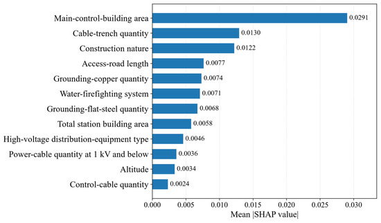
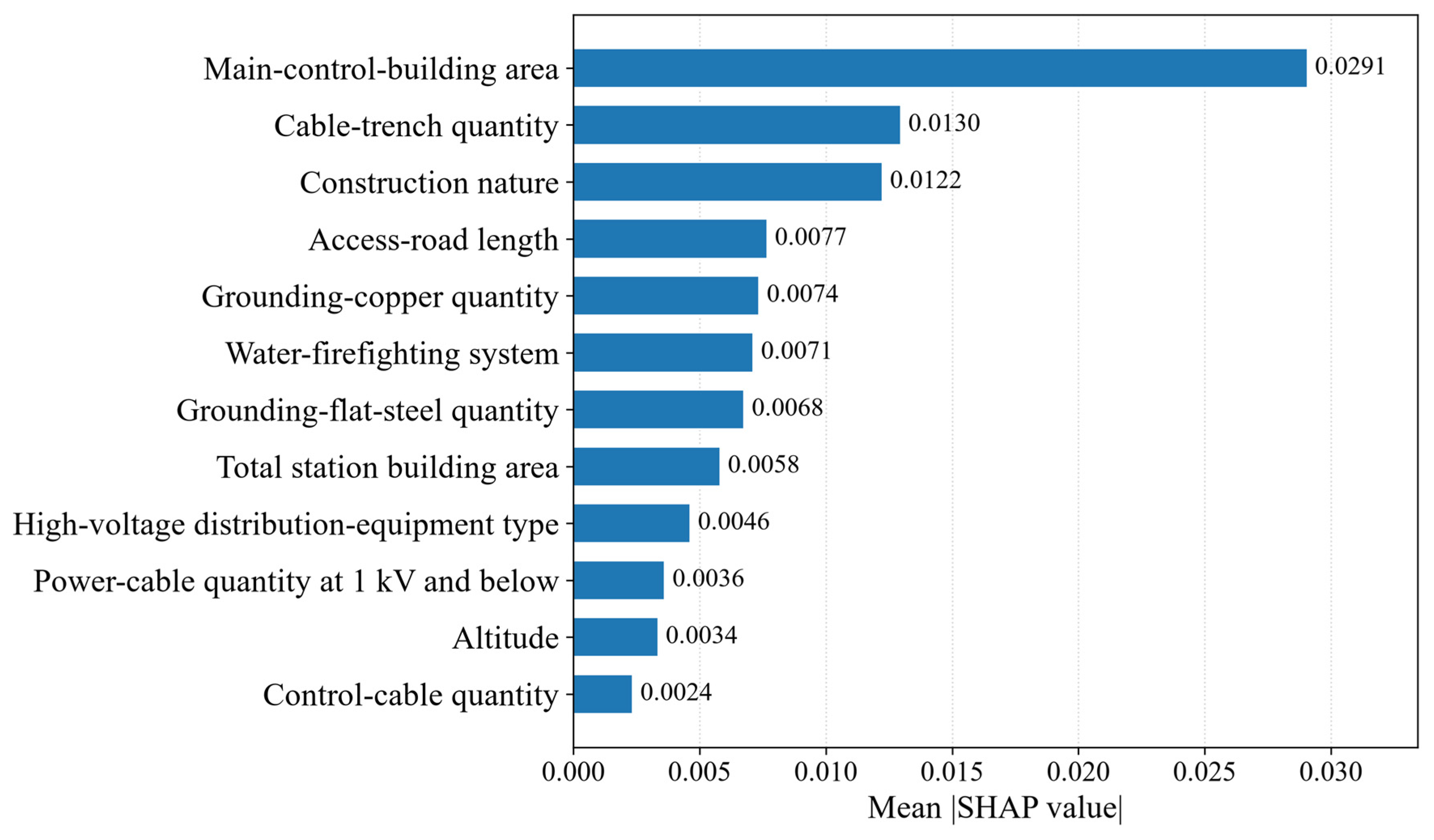
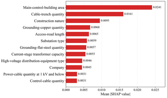
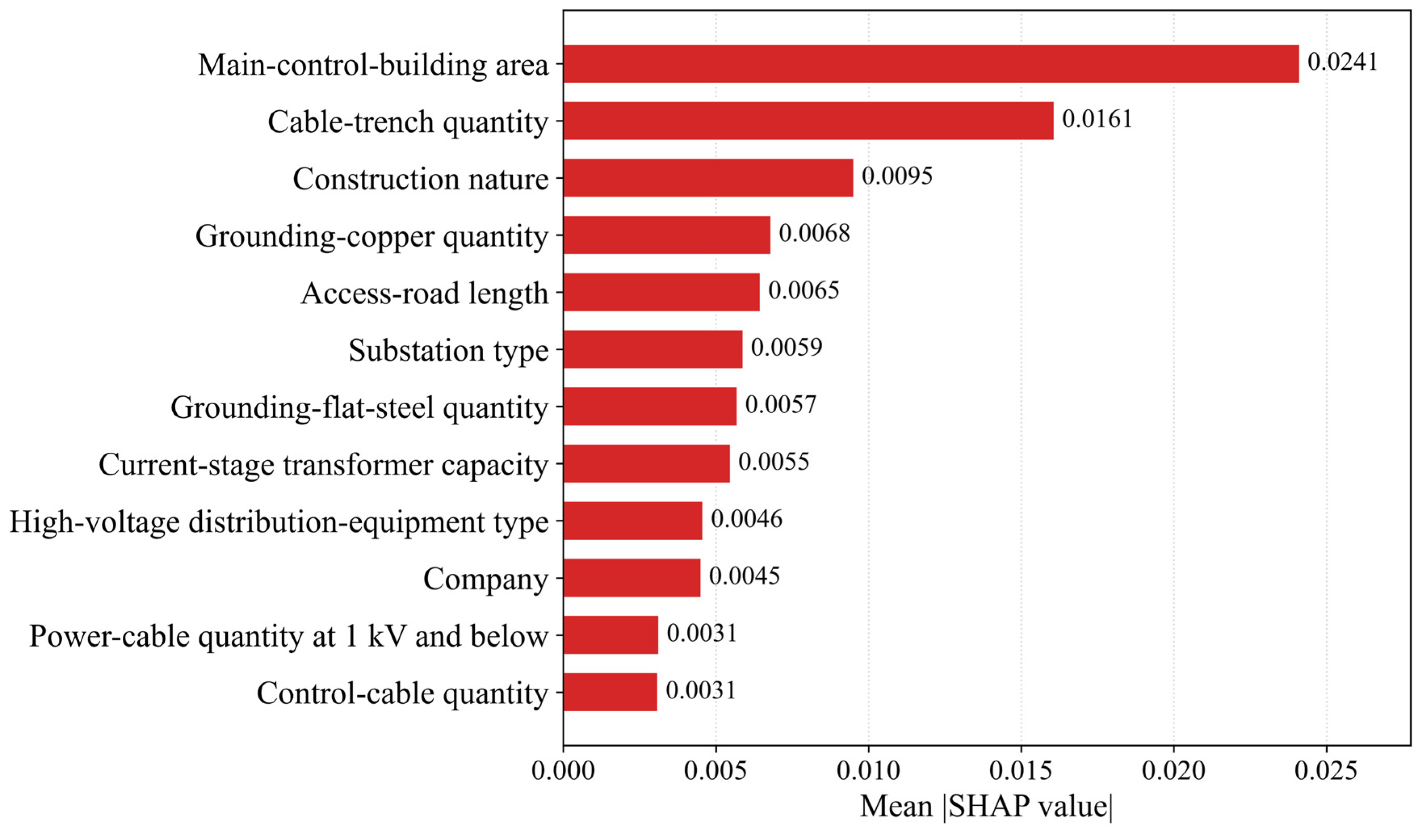
Global SHAP importance was evaluated for the Construction- and Equipment-share attribution proxy models across the 145 held-out projects (Figure 8 and Figure 9). Main-control-building area ranked as the most influential feature for both targets, while cable-trench quantity, construction nature, access-road length, and grounding-copper quantity were also highly ranked in both models. Although the two models therefore relied on a broadly similar set of civil-work and project-configuration features, their relative importance differed across the two Cost Structure components.

Figure 8. Global SHAP importance for the Construction-share attribution proxy model on the held-out test set.

Figure 9. Global SHAP importance for the Equipment-procurement-share attribution proxy model on the held-out test set.

4.6.2. Local SHAP Attribution for Project No. 1673

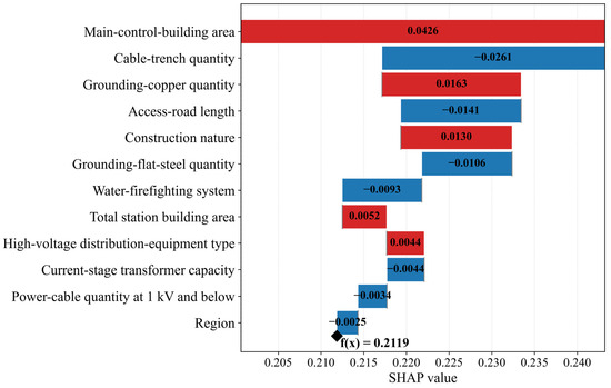
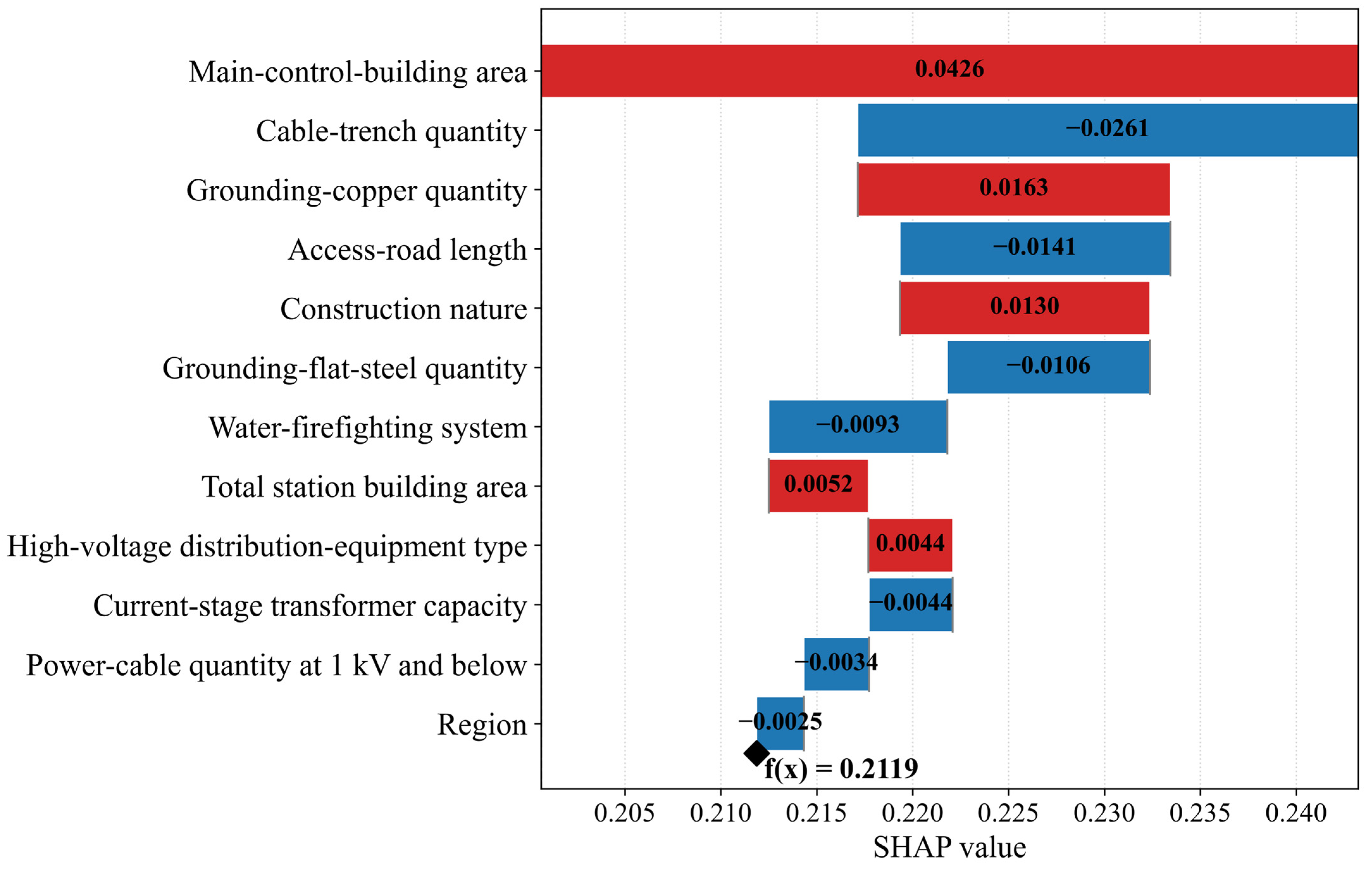
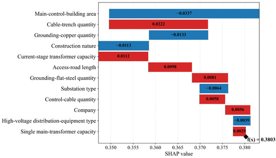
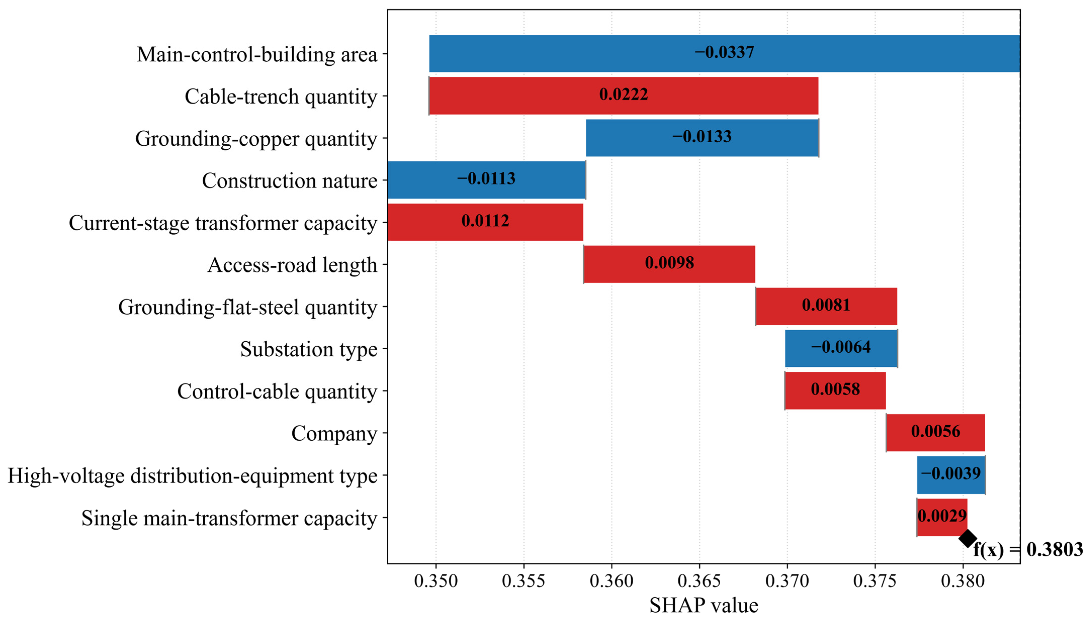
Local SHAP attribution was examined for Project No. 1673 using the Construction- and Equipment-share attribution proxy models. The proxy-model predictions were 22.68% for Construction and 47.18% for Equipment Procurement; these attribution-model outputs are distinct from the final closure-normalized Cost Structure point predictions reported in Table 18.

For the Construction-share proxy, main-control-building area provided the largest positive contribution, whereas the absence of cable-trench quantity and access-road length contributed negatively (Figure 10). In contrast, main-control-building area contributed negatively to the Equipment-share prediction, while the absence of cable-trench quantity and current-stage transformer capacity contributed positively (Figure 11). In Figure 10 and Figure 11, red bars indicate positive SHAP contributions, whereas blue bars indicate negative SHAP contributions. These opposite contribution patterns illustrate how shared engineering features can be used differently by the two target-specific attribution models. Because SHAP contributions are additive on the log-plus-one-transformed model-output scale, they are interpreted primarily by direction and relative magnitude rather than as direct percentage-point effects.

Figure 10. Local SHAP attribution for the Construction-share attribution proxy model of Project No. 1673.

Figure 11. Local SHAP attribution for the Equipment-procurement-share attribution proxy model of Project No. 1673.

Additional representative cases covering Total-cost, Unit-cost, Multi-dimension, and near-boundary unflagged screening patterns, together with their detailed SHAP attribution results, are provided in Supplementary Sections S8.2–S8.4 (Tables S18–S20).

5. Discussion

This study developed a multidimensional cost-deviation screening framework combining CatBoost point prediction, CQR uncertainty quantification, Cost Structure family-wise calibration, and SHAP feature attribution. CatBoost showed consistently competitive predictive performance across the three cost dimensions, achieving $R^2$ values of 0.9363 and 0.8899 for Total Cost and Unit Cost, respectively, and macro-average RMSE and MAE values of 3.70 and 2.63 percentage points for Cost Structure. The benchmark results support CatBoost as a common predictive backbone, although other models performed better on selected relative-error metrics. Relative to previous studies focusing separately on construction-cost point prediction [19], substation cost prediction [21], multioutput cost prediction [22], cost auditing [23], or explainable prediction [24], the present study integrates multidimensional cost representation, uncertainty-aware screening, multiplicity control, and post-screening attribution within one preliminary-design review workflow.

The marginal CQR intervals exhibited target-dependent coverage–width trade-offs rather than a uniform efficiency advantage over split conformal prediction. More importantly, simultaneous use of the five Cost Structure intervals required additional control of multiple screening signals. The economic-exposure-weighted family-wise calibration reduced the number of projects meeting the combined screening criterion from 59 under marginal screening to 22 after final dimensional screening. These comprised 10 Total-cost, 3 Unit-cost, 7 Cost-structure, and 2 Multi-dimension flags. Adding Cost Structure increased the overall flag rate from 10.34% to 15.17% and identified seven projects that were not flagged by Total Cost or Unit Cost alone, demonstrating that internal cost allocation provides incremental screening information beyond aggregate and capacity-normalized expenditure.

SHAP attribution provided complementary information after the screening decision had been established. The main-text Cost-structure example illustrated how common civil-work and project-configuration features could contribute differently to the Construction- and Equipment-share attribution-model outputs, while additional screening patterns are examined in Supplementary Section S8. The proxy-fidelity analysis supported the use of the attribution models for qualitative interpretation, although the proxies should not be regarded as replacements for the primary closure-normalized multi-output predictor.

From a practical perspective, the framework prioritizes projects and cost dimensions for subsequent engineering review, while SHAP provides feature-level context for checking design assumptions, engineering quantities, equipment configurations, and cost allocation.

The robustness analyses indicated limited sensitivity to random model initialization but revealed heterogeneity across voltage levels and review periods. Several limitations should be considered. First, the held-out evaluation involved projects from participating provincial grid companies, and audit-confirmed labels were unavailable; external and audit-linked validation is therefore needed. Second, some subgroups were small, and incomplete excluded records prevented a full retained-versus-excluded comparison. Third, the grouped CQR procedure provides an empirically evaluated rather than exact split-conformal guarantee, the Cost Structure intervals remain target-specific rather than fully compositional, and SHAP interpretation relies on attribution proxies. Future work should address these limitations through broader external validation, joint compositional uncertainty modeling, and attribution methods operating directly on the primary multi-output model.

6. Conclusions

This study developed a multidimensional cost-deviation screening framework for preliminary design estimates of power grid substation projects by integrating CatBoost point prediction, CQR prediction intervals, Cost Structure family-wise calibration, and SHAP feature attribution. The framework evaluates Total Cost, Unit Cost, and Cost Structure within a unified workflow for project-level screening and subsequent engineering review.

The framework was evaluated using 906 substation projects, including 761 projects for model development and 145 projects for held-out evaluation. CatBoost achieved $R^2$ values of 0.9363 for Total Cost and 0.8899 for Unit Cost, while the five-output Cost Structure model achieved macro-average RMSE and MAE values of 3.70 and 2.63 percentage points, respectively. The marginal CQR intervals achieved empirical coverage of 91.72% for Total Cost, 97.93% for Unit Cost, and 90.76% on average across the five Cost Structure targets. After Cost Structure family-wise calibration, 22 projects (15.17%) received final review flags, including 10 Total-cost, 3 Unit-cost, 7 Cost-structure, and 2 Multi-dimension flags. Adding Cost Structure increased the number of flagged projects from 15 to 22 and identified seven additional projects that were not flagged by Total Cost or Unit Cost alone. These results indicate that Cost Structure provides incremental screening information beyond aggregate Total Cost and capacity-normalized Unit Cost.

Overall, the empirical findings were broadly consistent with the four working hypotheses: CatBoost provided competitive predictive performance, CQR achieved generally appropriate but target-dependent empirical coverage, family-wise calibration reduced simultaneous Cost Structure screening signals, and Cost Structure contributed additional project-level screening information. SHAP attribution further provided feature-level context after screening. The framework should therefore be interpreted as a statistical review-prioritization tool rather than an automated determination of cost error.

References

- Bie, Z.; Lin, Y.; Li, G.; Li, F. Battling the Extreme: A Study on the Power System Resilience. Proc. IEEE 2017, 105, 1253–1266. [Google Scholar] [CrossRef] [Scilit]
- Mahzarnia, M.; Moghaddam, M.P.; Baboli, P.T.; Siano, P. A Review of the Measures to Enhance Power Systems Resilience. IEEE Syst. J. 2020, 14, 4059–4070. [Google Scholar] [CrossRef] [Scilit]
- Dursun, O.; Stoy, C. Conceptual Estimation of Construction Costs Using the Multistep Ahead Approach. J. Constr. Eng. Manag. 2016, 142, 04016038. [Google Scholar] [CrossRef] [Scilit]
- Elmousalami, H.H. Intelligent Methodology for Project Conceptual Cost Prediction. Heliyon 2019, 5, e01625. [Google Scholar] [CrossRef] [Scilit] [PubMed]
- Wang, Y.R.; Yu, C.Y.; Chan, H.H. Predicting Construction Cost and Schedule Success Using Artificial Neural Networks Ensemble and Support Vector Machines Classification Models. Int. J. Proj. Manag. 2012, 30, 470–478. [Google Scholar] [CrossRef] [Scilit]
- Chakraborty, D.; Elhegazy, H.; Elzarka, H.; Gutierrez, L. A Novel Construction Cost Prediction Model Using Hybrid Natural and Light Gradient Boosting. Adv. Eng. Inform. 2020, 46, 101201. [Google Scholar] [CrossRef] [Scilit]
- Son, H.; Kim, C.; Kim, C. Hybrid Principal Component Analysis and Support Vector Machine Model for Predicting the Cost Performance of Commercial Building Projects Using Pre-Project Planning Variables. Autom. Constr. 2012, 27, 60–66. [Google Scholar] [CrossRef] [Scilit]
- Shutian, F.; Tianyi, Z.; Ying, Z. Prediction of Construction Projects’ Costs Based on Fusion Method. Eng. Comput. 2017, 34, 2396–2408. [Google Scholar] [CrossRef] [Scilit]
- Wood, A.J.; Wollenberg, B.F.; Sheblé, G.B. Power Generation, Operation, and Control; John Wiley & Sons: Hoboken, NJ, USA, 2013. [Google Scholar]
- Zhao, L.; Mbachu, J.; Liu, Z. Identifying Significant Cost-Influencing Factors for Sustainable Development in Construction Industry Using Structural Equation Modelling. Math. Probl. Eng. 2020, 2020, 4810136. [Google Scholar] [CrossRef] [Scilit]
- Zhao, L.; Wang, B.; Mbachu, J.; Liu, Z. New Zealand Building Project Cost and Its Influential Factors: A Structural Equation Modelling Approach. Adv. Civ. Eng. 2019, 2019, 1362730. [Google Scholar] [CrossRef] [Scilit]
- Jung, W.; Han, S.H. Which Risk Management Is Most Crucial for Controlling Project Cost? J. Manag. Eng. 2017, 33, 04017029. [Google Scholar] [CrossRef] [Scilit]
- Huang, C.H.; Hsieh, S.H. Predicting BIM Labor Cost with Random Forest and Simple Linear Regression. Autom. Constr. 2020, 118, 103280. [Google Scholar] [CrossRef] [Scilit]
- Cingillioglu, I.; Bowles, N.; Mitchell, N.; Rinne, M. A Comparative Analysis of Machine Learning Algorithms for Predicting South Australian Electricity Prices. J. Bus. Anal. 2025, 1–16. [Google Scholar] [CrossRef] [Scilit]
- Ma, M.; Tam, V.W.Y.; Le, K.N.; Osei-Kyei, R. A Systematic Literature Review on Price Forecasting Models in Construction Industry. Int. J. Constr. Manag. 2024, 24, 1191–1200. [Google Scholar] [CrossRef] [Scilit]
- Ahiaga-Dagbui, D.D.; Smith, S.D. Dealing with Construction Cost Overruns Using Data Mining. Constr. Manag. Econ. 2014, 32, 682–694. [Google Scholar] [CrossRef] [Scilit]
- Breiman, L.; Friedman, J.; Olshen, R.A.; Stone, C.J. Classification and Regression Trees; Chapman and Hall/CRC: Boca Raton, FL, USA, 2017. [Google Scholar] [CrossRef] [Scilit]
- Ribeiro, M.T.; Singh, S.; Guestrin, C. Why Should I Trust You? Explaining the Predictions of Any Classifier. In Proceedings of the 22nd ACM SIGKDD International Conference on Knowledge Discovery and Data Mining, San Francisco, CA, USA, August 2016; Association for Computing Machinery: New York, NY, USA, 2016; pp. 1135–1144. [Google Scholar] [CrossRef] [Scilit]
- Park, U.; Kang, Y.; Lee, H.; Yun, S. A stacking heterogeneous ensemble learning method for the prediction of building construction project costs. Appl. Sci. 2022, 12, 9729. [Google Scholar] [CrossRef] [Scilit]
- Wang, R.; Asghari, V.; Cheung, C.M.; Hsu, S.-C.; Lee, C.-J. Assessing effects of economic factors on construction cost estimation using deep neural networks. Autom. Constr. 2022, 134, 104080. [Google Scholar] [CrossRef] [Scilit]
- Xu, X.; Peng, L.; Ji, Z.; Zheng, S.; Tian, Z.; Geng, S. Research on substation project cost prediction based on sparrow search algorithm optimized BP neural network. Sustainability 2021, 13, 13746. [Google Scholar] [CrossRef] [Scilit]
- Yun, S. Performance analysis of construction cost prediction using neural network for multioutput regression. Appl. Sci. 2022, 12, 9592. [Google Scholar] [CrossRef] [Scilit]
- Wang, P.; Wang, K.; Huang, Y.; Fenn, P.; Stewart, I. Auditing construction cost from an in-process perspective based on a Bayesian predictive model. J. Constr. Eng. Manag. 2022, 148, 04022003. [Google Scholar] [CrossRef] [Scilit]
- Chen, L.; Xu, C.; Lim, W.H.; Sharma, A.; Tiang, S.S.; Chong, K.S.; El-Kenawy, E.-S.M.; Alhussan, A.A.; Eid, M.M.; Khafaga, D.S. Transparent and reliable construction cost prediction using advanced machine learning and explainable AI. Eng. Sci. Technol. Int. J. 2025, 70, 102159. [Google Scholar] [CrossRef] [Scilit]
- Prokhorenkova, L.; Gusev, G.; Vorobev, A.; Dorogush, A.V.; Gulin, A. CatBoost: Unbiased Boosting with Categorical Features. Adv. Neural Inf. Process. Syst. 2018, 31, 6638–6648. [Google Scholar]
- Dorogush, A.V.; Ershov, V.; Gulin, A. CatBoost: Gradient Boosting with Categorical Features Support. arXiv 2018, arXiv:1810.11363. [Google Scholar] [CrossRef] [Scilit]
- Huang, G.; Wu, L.; Ma, X.; Zhang, W.; Fan, J.; Yu, X.; Zhou, H. Evaluation of CatBoost Method for Prediction of Reference Evapotranspiration in Humid Regions. J. Hydrol. 2019, 574, 1029–1041. [Google Scholar] [CrossRef] [Scilit]
- Hancock, J.T.; Khoshgoftaar, T.M. CatBoost for Big Data: An Interdisciplinary Review. J. Big Data 2020, 7, 94. [Google Scholar] [CrossRef] [Scilit] [PubMed]
- Romano, Y.; Patterson, E.; Candès, E. Conformalized Quantile Regression. Adv. Neural Inf. Process. Syst. 2019, 32, 3543–3553. [Google Scholar]
- Sesia, M.; Candès, E.J. A Comparison of Some Conformal Quantile Regression Methods. Stat 2020, 9, e261. [Google Scholar] [CrossRef] [Scilit]
- Jensen, V.; Bianchi, F.M.; Anfinsen, S.N. Ensemble Conformalized Quantile Regression for Probabilistic Time Series Forecasting. IEEE Trans. Neural Netw. Learn. Syst. 2022, 35, 9014–9025. [Google Scholar] [CrossRef] [Scilit] [PubMed]
- Lundberg, S.M.; Lee, S.I. A Unified Approach to Interpreting Model Predictions. Adv. Neural Inf. Process. Syst. 2017, 30, 4765–4774. [Google Scholar]
- Štrumbelj, E.; Kononenko, I. Explaining Prediction Models and Individual Predictions with Feature Contributions. Knowl. Inf. Syst. 2014, 41, 647–665. [Google Scholar] [CrossRef] [Scilit]
- Lundberg, S.M.; Erion, G.G.; Lee, S.I. Consistent Individualized Feature Attribution for Tree Ensembles. arXiv 2018, arXiv:1802.03888. [Google Scholar] [CrossRef] [Scilit]
- Shapley, L.S. A Value for N-Person Games. In Contributions to the Theory of Games II; Princeton University Press: Princeton, NJ, USA, 1953; pp. 307–318. [Google Scholar]
- Guidotti, R.; Monreale, A.; Ruggieri, S.; Turini, F.; Giannotti, F.; Pedreschi, D. A Survey of Methods for Explaining Black Box Models. ACM Comput. Surv. 2018, 51, 93. [Google Scholar] [CrossRef] [Scilit]
Disclaimer/Publisher’s Note: The statements, opinions and data contained in all publications are solely those of the individual author(s) and contributor(s) and not of MDPI and/or the editor(s). MDPI and/or the editor(s) disclaim responsibility for any injury to people or property resulting from any ideas, methods, instructions or products referred to in the content. |
© 2026 by the authors. Licensee MDPI, Basel, Switzerland. This article is an open access article distributed under the terms and conditions of the Creative Commons Attribution (CC BY) license.