Day-Ahead XGBoost Forecasting of Aggregated Residential Load: Accuracy and SHAP Ranking Agreement Across Experimental Configurations

Abstract

This study assessed how the selected seasonal test period, training-window strategy, and hyperparameter selection were associated with differences in XGBoost day-ahead forecast accuracy and interpretation for approximately 300 G11-tariff households in Poland. Sixteen configurations combined four 31-day periods, sliding or expanding training windows, and shared (H1) or window-specific (H2) hyperparameters. The model used 19 temporal, meteorological, and calendar features; meteorological predictors for training, validation, and testing were archived numerical weather prediction (NWP) forecasts from the same operational forecasting system, available before the forecasted day. Accuracy was evaluated using mean absolute error (MAE), root mean square error (RMSE), and mean absolute percentage error (MAPE); paired comparisons used the Diebold–Mariano test with the Harvey–Leybourne–Newbold correction and Holm adjustment. Global SHAP (SHapley Additive exPlanations) rankings were compared using Spearman’s coefficient. MAE ranged from 7.79 to 14.98 kWh, and all configurations had lower MAE, RMSE, and MAPE than both persistence benchmarks. After Holm correction, no training-window strategy showed a statistically supported advantage; H2 was supported for the autumn expanding-window comparison, whereas the summer result depended on the variance estimator. The 24 h consumption lag ranked first in every configuration, and mean rank agreement across 120 pairs was 0.897. Accuracy varied across periods and configurations, whereas feature hierarchy remained highly consistent.

1. Introduction

1.1. Research Context and Motivation

Short-term load forecasting is an important component of power system operation, particularly given the growing share of renewable energy sources and the variability of consumer behavior. Accurate short-term forecasts support balancing, grid operation, and operational decisions whose importance grows with the development of distributed generation, storage, and demand-side flexibility [1,2,3,4,5].

The load profiles of households and low-voltage consumers are shaped by daily and weekly rhythms, season, weather, and user behavior [3,6]. Aggregation attenuates part of the variability inherent to individual households [7], but it does not eliminate the nonlinearity and non-stationarity of the process [2,3]. Our previous study compared forecasting methods for the same aggregated profile of approximately 300 residential consumers in the Polish G11 tariff group in Gliwice [8].

Unlike the demand of an entire power system, the profile of a local consumer group is more strongly affected by calendar events and by the synchronization of daily behaviors. Even after aggregation, short-lived deviations may occur that are invisible in monthly averages, and their operational significance depends on the hour and the direction of the error. Evaluation of short-term load forecasting (STLF) should therefore encompass not only a single metric aggregated over the whole period but also the temporal distribution of errors.

Load forecasting relies on consumption history, calendar features, and meteorological variables whose relevance may depend on the time of day and the season of the year [2,6,9,10]. Lag features and rolling statistics capture the memory and local variability of the process [11,12]. Alongside naive methods, regression, and classical time-series models, including ARIMA [1,2,11,13], machine learning models capable of representing nonlinear dependencies are used [12]; schemes that separately identify peak loads have also been examined [14]. Greater model flexibility, however, increases the need to interpret model predictions [3].

The reported error depends not only on the algorithm but also on the test period, the training-window update strategy, and the hyperparameter tuning strategy. For a seasonal and non-stationary process, these decisions govern the trade-off between data recency, history length, and computational cost. Although seasonality is sometimes accounted for by constructing separate models [15], controlled comparisons of several design decisions remain rare, which limits the comparability of results [3].

A sliding window discards the oldest observations and preserves a fixed sample size, whereas an expanding window retains the entire available history. The former can respond faster to process change; the latter can reduce estimation variance and reinforce less frequently observed patterns. Similarly, selecting hyperparameters separately for different training windows may match model complexity to the current window but increases cost and the risk of overfitting the choice to a particular validation realization. The relative effectiveness of these strategies therefore cannot be established from theory alone.

1.2. Machine Learning and Interpretability in Load Forecasting

XGBoost effectively represents nonlinearities and interactions and is therefore widely used in load forecasting [2,16,17,18,19]. It can combine historical, meteorological, and calendar predictors [2,3,9,12,19], but it requires explicit engineering of temporal features [19].

An advantage of the model is its ability to represent thresholds and interactions without imposing their functional form a priori. At the same time, the outcome depends on the number and depth of trees, the learning rate, observation and feature subsampling, and regularization. Evaluating the effect of a tuning strategy therefore requires separating the validation score, the quality on an independent test period, and the computational cost; the lowest MAE (mean absolute error) on the grid does not guarantee an advantage after deployment.

In power system applications, interpretability supports model verification and audit [3,20], particularly for black-box methods [20,21].

SHAP (SHapley Additive exPlanations) is an explainable artificial intelligence (XAI) method based on Shapley values [22,23] that attributes contributions to individual predictions and enables both global and local analysis [23]. For tree-based models, TreeSHAP provides an efficient computation of additive attributions [24] that are also used in energy forecasting [20,25].

Attributions, however, explain the fitted model rather than the causal mechanism of the process. Different, similarly accurate models may distribute feature importance differently [26]; the stability and uncertainty of explanations therefore require separate evaluation [27,28]. SHAP-based rankings may differ between datasets describing similar systems [25], while in load forecasting the ranking of a single model is most often reported [29,30]. This raises the question of whether the feature hierarchy is robust to the decisions that shape the experimental setup.

Ranking stability has a different meaning than the stability of an individual forecast or a local attribution. A high rank correlation may coexist with a change in the absolute scale of SHAP values, a change in the direction of influence over part of the range, or a change in the explanation of a specific observation. For this reason, the global analysis in this study is complemented by attribution distributions, dependence plots, and local cases.

1.3. Research Gap and Contributions

Previous studies have used SHAP to interpret load forecasting models [25,29,31], in parallel developing inherently more transparent models [32,33] and using XAI in feature selection [34]. Rarely, however, has it been examined whether the global SHAP-based ranking remains consistent across models that differ in test period, window strategy, and tuning strategy. This study addresses this gap through a structured comparison of 16 XGBoost configurations. Its contribution lies in the experimental-design analysis rather than in the development of a new forecasting algorithm, jointly examining forecast accuracy and global TreeSHAP-ranking agreement across predefined test periods, training-window strategies, and one-time hyperparameter-selection strategies. Ranking agreement describes the robustness of the interpretation within this procedure but does not prove the causal significance of the features.

The gap has two related dimensions. First, comparisons of accuracy often vary the data period, the length of the history, and the tuning procedure simultaneously, which makes it difficult to distinguish an algorithmic benefit from an experimental design effect. Second, the interpretation is usually presented for a single chosen model, without checking whether the conclusion about the most important predictors holds after the same decisions are changed. The matrix used in this work makes it possible to assess both issues on a common profile and under a uniform day-ahead forecasting protocol.

On this basis, two research questions are formulated:

1.

To what extent does the accuracy of hourly electricity consumption forecasts vary across the four selected 31-day seasonal test periods, the two training-window update strategies, and the two hyperparameter-selection strategies, and are the differences associated with the window strategy and the hyperparameter selection strategy statistically distinguishable?

2.

To what extent are the global SHAP-based feature importance rankings consistent across configurations that differ in selected seasonal test period, training-window update strategy, and hyperparameter selection strategy?

This study uses the hourly aggregated profile of approximately 300 G11 households in Gliwice, analyzed previously in a comparison of forecasting methods [8]. For 19 predictors and 16 configurations, walk-forward day-ahead forecasts, an accuracy evaluation, and a TreeSHAP analysis were carried out. The matrix enables the comparison of complete experimental strategies but does not identify isolated causal effects.

The main elements of the contribution are as follows:

• A walk-forward comparison of 16 XGBoost configurations combining four selected 31-day seasonal test periods, two training-window strategies, and two hyperparameter-selection strategies with parameters fixed throughout each test period;
• A paired evaluation of forecast differences using the Diebold–Mariano test, complemented by effect sizes and confidence intervals;
• A quantitative assessment of TreeSHAP-ranking agreement across configurations, complemented by bootstrap and multi-seed sensitivity analyses.

The overall structure of the study is summarized in Figure 1.

2. Materials and Methods

2.1. Study Area and Data Sources

The study concerns the aggregated hourly electricity consumption of approximately 300 residential households in the Polish single-zone G11 tariff group in Gliwice, southern Poland [8]. The distribution system operator provided an aggregated time series without data from individual meters. The target variable is the hourly electricity consumption of the entire group [kWh]; the main characteristics of the dataset are summarized in

Table 1. General characteristics of the electricity consumption dataset.

Characteristic	Dataset Details
Data period and resolution	1 January 2023–31 December 2024; 1 h
Number of records	17,544 source records; 17,376 complete feature records
Data completeness	No gaps, missing values, or duplicate timestamps
Consumer group	Approx. 300 residential households in the G11 tariff group
Target variable	Aggregated hourly electricity consumption [kWh]
Distribution	Mean ± SD: 165.06 ± 62.26 kWh; median [Q1–Q3]: 149.12 [115.37–201.94] kWh; range: 66.42–415.54 kWh

.

The source series covers 731 days and contains no gaps, missing values, or duplicate timestamps. After generating the historical features, 17,376 complete rows remained. The two-year period provides at least one year of history before each test period and covers daily, weekly, and seasonal variability [3]. The load profile is shaped by activity rhythms and seasonal conditions [3,6,10]. In contrast to the earlier comparison of forecasting algorithms for the same consumer group [8], the present study uses these data to assess the dependence of XGBoost accuracy and SHAP attributions on the experimental configuration.

Meteorological and calendar variables represent weather conditions and consumer activity cycles [6,9,10]. Each electricity-consumption observation was matched with meteorological and calendar data at hourly resolution. All meteorological predictors used during model training, validation, and testing were archived numerical weather prediction (NWP) forecast values obtained from the same external operational forecasting system. The system updates its forecasts automatically several times per day and provides forecast horizons of up to 10 days. For the day-ahead workflow, a forecast snapshot was typically retrieved at approximately 08:00–09:00 on day N, and the hourly meteorological values for the complete day N + 1 were used as inputs to the load-forecasting model. A single meteorological forecast series representative of Gliwice was assigned to the entire aggregated consumer group. The exact model issue time associated with individual archived forecast snapshots, the exact update interval, the underlying NWP grid resolution, and the provider-side spatial aggregation or interpolation procedure were not available in the retained technical documentation. The provider cannot be disclosed under the data-access terms. Calendar variables were known in advance.

The source data were supplied in local time on a regular 24 h daily grid. According to the data provider’s convention, during the autumn daylight-saving-time transition, when the local day contains 25 h, the additional hourly observation was removed. During the spring transition, when the local day contains 23 h, the missing hourly observation was reconstructed by the provider as the arithmetic mean of the immediately preceding and following hourly observations. These adjustments were performed by the provider before the data were delivered; no additional time-zone or DST correction was applied by the authors.

The source timestamps marked the end of each hourly interval; for reporting and interpretation of the hourly results, they were displayed one hour earlier so that hours 0–23 denote interval start times. The variables month, day_of_week, and day_off were not recomputed according to this reporting convention and therefore refer to the following date for records displayed as 23:00. This affects 4.17% of day_of_week values, 0.13% of month values, and 1.08–1.34% of day_off values within a 31-day configuration. The convention does not cause data leakage because all calendar variables were available before forecasting, but it creates a limited semantic mismatch in their interpretation at the day boundary when records are expressed using interval-start timestamps. The same convention was applied consistently in all 16 experimental configurations.

The precipitation variable represents the precipitation amount accumulated during the preceding hour, consistent with the source-data definition and the end-of-interval timestamp convention described above. The formula for heat_index was not retained; this variable was identical to temperature in all winter, spring, and autumn observations and in 600 of the 744 summer observations, with a summer correlation of approximately 0.9974. It was retained to reproduce the original experiment. Because of this near redundancy, heat_index and temperature should not be interpreted as independent physical drivers, and their individual SHAP attributions may be redistributed between correlated predictors. An ablation variant excluding heat_index would constitute a different model specification and is therefore treated as a sensitivity-analysis direction rather than as a retrospective modification of the evaluated 19-feature experiment. Pressure values used by the model ranged from approximately 98 to 104 kPa; in the waterfall plot they were converted to hPa for presentation.

2.2. Data Preprocessing and Input Feature Engineering

The electricity-consumption, meteorological, and calendar streams were merged chronologically at hourly resolution. Completeness and temporal consistency were verified before feature generation because disturbances in input data may affect forecasting accuracy and robustness [13]. After receipt of the provider-standardized series, variables were converted to numeric form, and neither additional imputation nor automatic outlier removal was applied by the authors because the source series was complete. Observations were not shuffled, no transformations were estimated on the full dataset, and historical predictors were computed only from values available before the forecasted day. The same 19-feature set was used in all configurations.

Three lag features represented the temporal memory of the load: lag_24, lag_48, and lag_168, corresponding to consumption at the same hour one day, two days, and one week earlier, respectively [8,11,12,19]. Shorter lags such as lag_1 and lag_2 were omitted because, when the complete 24 h profile is forecast before the start of the day, these values are unavailable for most forecasted hours. Thus, lag_24 is the most recent target history available for every hour of the day-ahead forecast.

Two rolling statistics were calculated from the 24 observations in the interval $[t-48,t-25]$: rolling_mean_24 and rolling_std_24. They complement the lag features with information on the recent load level and variability [3]. The offset ensures that the complete window lies before the forecasted day and is available for all 24 forecast hours. After removing the first 168 records lacking sufficient history, the complete feature dataset covered 8 January 2023, 00:00–31 December 2024, 23:00.

Table 2. Complete set of input features used by the XGBoost model.

Feature	Group	Unit or Definition	Description
lag_24	Temporal	$y(t-24)$	Consumption at the same hour of the previous day
lag_48	Temporal	$y(t-48)$	Consumption at the same hour two days earlier
lag_168	Temporal	$y(t-168)$	Consumption at the same hour one week earlier
rolling_mean_24	Temporal	Mean over $[t-48,t-25]$	Previous-day load level
rolling_std_24	Temporal	SD over $[t-48,t-25]$	Previous-day load variability
temperature	Meteorological	°C	Air temperature
humidity	Meteorological	%	Relative humidity
wind_speed	Meteorological	m/s	Wind speed
wind_direction	Meteorological	°	Wind direction
cloud_cover	Meteorological	%	Cloud cover
precipitation	Meteorological	mm	Previous-hour precipitation
radiation	Meteorological	W/m2	Direct solar irradiance
wind_chill	Meteorological	°C	Wind chill
heat_index	Meteorological	°C	Heat index
pressure	Meteorological	kPa	Atmospheric pressure
hour	Calendar	0–23	Hour at the start of the interval
day_of_week	Calendar	1–7	Day of week
month	Calendar	1–12	Month
day_off	Calendar	{0, 1}	Non-working-day indicator

Note: All meteorological predictors used during training, validation, and testing were archived NWP forecast values from the same operational forecasting system.

summarizes the full set of five historical, ten meteorological, and four calendar predictors.

2.3. XGBoost Forecasting Model

The regularized gradient-boosted tree algorithm XGBoost [16] was applied, which is suitable for nonlinear dependencies and interactions [16,18]. Its usefulness in load forecasting is confirmed by previous studies [8,19].

The forecasting of hourly electricity consumption was formulated as a regression task: for each time point t, the model generates a prediction $\widehat{y}\left(t\right)$ of the actual consumption $y\left(t\right)$ [kWh] based on the vector of input features $\mathbf{x}\left(t\right)$ described in Section 2.2. The objective function minimized by XGBoost has the form:

$$\mathcal{L}\left(\varphi \right)={\displaystyle \sum _{i=1}^n}l\left(y_i,{\widehat{y}}_i\right)+{\displaystyle \sum _{k=1}^K}\mathrm{\Omega }\left(f_k\right),$$

(1)

where $l(y_i,{\widehat{y}}_i)={\displaystyle \frac{1}{2}}{(y_i-{\widehat{y}}_i)}^2$ is the squared loss appropriate for a regression problem (objective: reg:squarederror), $f_k$ denotes the k-th tree among the K component trees, and the regularization term $\mathrm{\Omega }\left(f_k\right)=\gamma T_k+{\displaystyle \frac{1}{2}}\lambda {\parallel w_k\parallel }^2$ penalizes excessive model complexity by constraining the number of leaves $T_k$ and the squared norm of the leaf weights $w_k$, where $\gamma$ and $\lambda$ are regularization hyperparameters [16]. In accordance with the experimental documentation, the same fixed random seed (random state) was used in all 16 configurations for elements involving random sampling (subsample, colsample_bytree). During the revision, the training code was recovered and confirmed that the random-state value used in the original procedure was 42. The serialized models from the original experiment were not retained; however, the recovered code enabled an additional multi-seed sensitivity analysis described in Section 2.5.

In the recovered implementation, the XGBoost estimator used objective=reg:squarederror, random_state=42, verbosity=0, and n_jobs=-1; the six optimized hyperparameters are reported in

Table 3. Hyperparameter search space of the XGBoost model. The grid contains $3\times 3\times 3\times 2\times 2\times 2=216$ combinations; the selected values—one shared set for the H1 strategy and eight sets (one per window) for the H2 strategy—are reported in the Results Section (Section 3.1).

Hyperparameter	Search Range	Description
n_estimators	{100, 300, 500}	Number of component trees in the ensemble
max_depth	{3, 5, 7}	Maximum depth of an individual tree
learning_rate	{0.01, 0.05, 0.1}	Learning rate (shrinkage); scales the contribution of each subsequent tree
subsample	{0.8, 1.0}	Fraction of observations sampled at random for each tree
colsample_bytree	{0.8, 1.0}	Fraction of features sampled at random for each tree
gamma	{0, 0.5}	Minimum required loss-reduction gain for a node split

, while the remaining estimator arguments were left at their library defaults. The revision-time verification and sensitivity analyses were performed using Python 3.14, Anaconda Navigator 2.7.1, Spyder 5.4.3, XGBoost 3.2.0, scikit-learn 1.2.2, NumPy 1.26.4, pandas 2.1.4, SciPy 1.11.4, Matplotlib 3.8.0, and openpyxl 3.0.10. This software specification refers to the revision-time analyses and should not be interpreted as a reconstruction of the complete historical runtime environment of the original experiment.

In this work, a single global XGBoost model was used, covering the forecasting of electricity consumption for all hours of the day. The information about the hour for which the forecast is issued is represented by the calendar input variable hour (Table 2), which allows the model to capture the specificity of individual hours without the need to train separate hourly models, in contrast to the scheme used in our previous study [8].

Six hyperparameters were optimized, specifying the number and depth of trees, the learning rate, the sampling of observations and features, and the minimum split gain (Table 3).

The grid was searched with five chronological TimeSeriesSplit folds, minimizing the validation MAE (mean absolute error). In case of ties, the first configuration in the deterministic grid order was selected. H1 was tuned once on a shared 2023 window, whereas H2 hyperparameters were selected once for each of the eight configurations using its initial training window; the selected parameters remained fixed for the test period. The ${\mathrm{MAE}}_{CV}$ values serve solely for selection within a given window, and the H1–H2 comparison also encompasses differences in the scope and recency of the validation data. The construction remains consistent with the general scheme of our previous study [8]. The chronological cross-validation splitter was instantiated as TimeSeriesSplit(n_splits=5), with no additional splitter arguments specified. Together with the tuning-window boundaries specified in Section 2.4 and

Table 4. Test periods and training windows for the four seasons under both window strategies. The test periods (31 days) are common to the sliding and expanding strategies.

Season	Test Period (2024)	Sliding Window (365 Days)	Effective Expanding Window (from 8 January 2023)
Winter	15 January–14 February	15 January 2023–14 January 2024	8 January 2023–14 January 2024 (372 days; 8928 observations)
Spring	15 April–15 May	15 April 2023–14 April 2024	8 January 2023–14 April 2024 (463 days; 11,112 observations)
Summer	15 July–14 August	15 July 2023–14 July 2024	8 January 2023–14 July 2024 (554 days; 13,296 observations)
Autumn	15 October–14 November	15 October 2023–14 October 2024	8 January 2023–14 October 2024 (646 days; 15,504 observations)

, this deterministically defines the training and validation splits used for hyperparameter selection.

2.4. Experimental Design

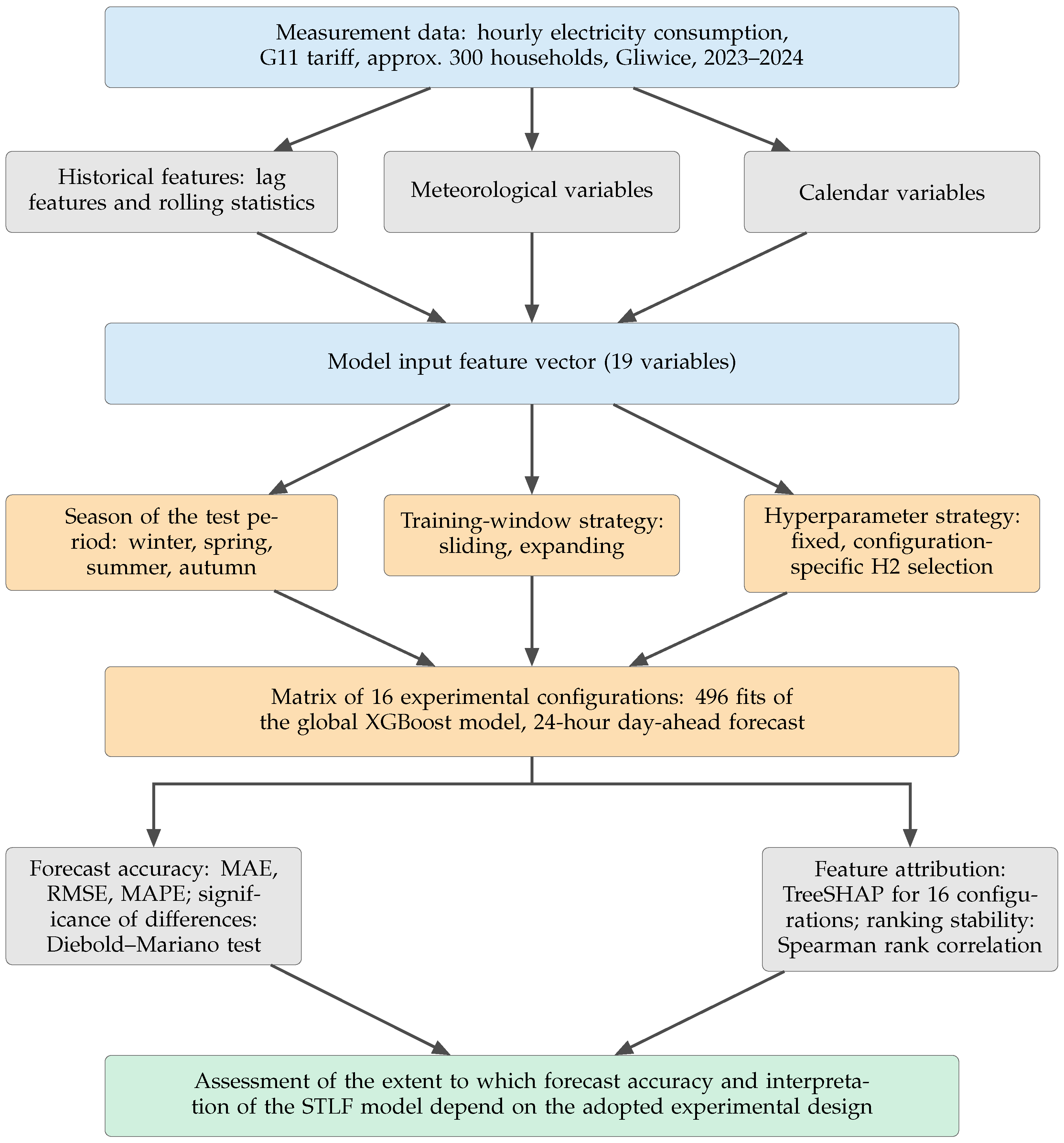
The study was designed as a systematic comparison of three dimensions of methodological decisions related to forecast accuracy and to the stability of SHAP (SHapley Additive exPlanations) model interpretation. In all configurations, the same XGBoost model class (Section 2.3), the same 19-element input feature space (Section 2.2), and the same daily forecast horizon (24 h, day-ahead) were used. Keeping these elements fixed makes it possible to link the observed differences to the experimental strategies being compared, but does not amount to identification of isolated causal effects. In particular, the seasonal period represents a specific month, the window strategies differ simultaneously in sample size and sample age, and the H1 and H2 strategies differ in the scope and recency of the data used for tuning.

The factors considered define an experimental configuration matrix with three dimensions:

• Selected seasonal test period (four levels: winter, spring, summer, autumn)—Each level is represented by a 31-day test period in 2024, preceded by at least one year of training material; the four periods are treated as distinct test realizations rather than replicated estimates of a general seasonal effect;
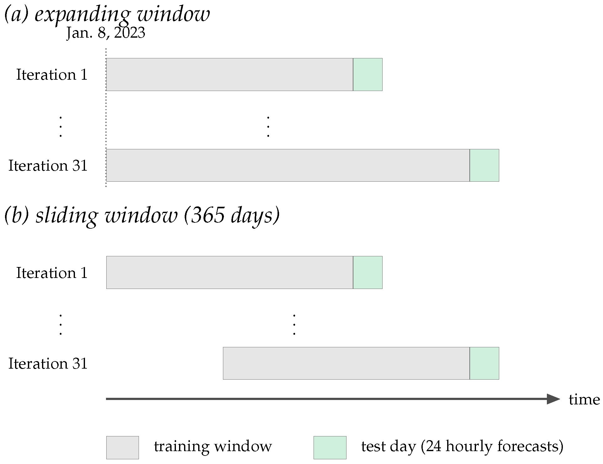
• Training-window strategy (two levels): Sliding—A window of fixed length of 365 days, covering a full annual cycle and shifted with the progress of the simulation; expanding—a window anchored at the first complete feature row, i.e., 8 January 2023, and growing monotonically (the mechanics of walk-forward retraining are described in Section 2.5). The comparison concerns these two specific strategies of managing the data history; other lengths of the sliding window were not analyzed.
• Hyperparameter tuning strategy (two levels): H1—A shared configuration determined once on 2023 data and used in all configurations of this group; H2—a configuration determined separately on the initial training window of each configuration (Section 2.3). These are two complete tuning strategies, which also differ in the recency and scope of the data used for validation.

The product of the levels of all three dimensions ($4\times 2\times 2$) yields 16 experimental configurations. The hyperparameter values for the H1 strategy were determined once by grid search on 2023 data (1 January 2023–31 December 2023) and applied without modification in all eight configurations of this group; in the H2 strategy, tuning was carried out independently on the training window of each of the eight configurations. The range 1 January 2023–31 December 2023 is the nominal series range for H1 tuning; after feature generation, the complete observations available for estimation begin on 8 January 2023.

The dates of the test periods and of the corresponding effective training windows for both strategies are compiled in Table 4. The test periods are identical for sliding and expanding within the same season, which removes the difference on the test-set side. The comparison does not, however, isolate the abstract principle of window updating itself, since the strategies differ simultaneously in the retention of older observations, in training sample size, and in data age. The results should therefore be referred to specific strategies: a one-year sliding window and an expanding window from the first complete feature row, i.e., 8 January 2023.

The choice of the range of history used for estimation is an important element of the forecasting procedure under conditions of possible process instability. An expanding window increases the sample size but also retains older observations, whereas a sliding window limits the influence of outdated data at the cost of a smaller sample. The literature indicates that the choice between these strategies reflects a trade-off between bias and variance of the forecast error and is not universal in nature [35,36]. For this reason, the window strategy was treated as a separate dimension of the comparison rather than adopting one of the strategies as the default.

The full matrix of 16 configurations, together with the adopted labels, is listed in

Table 5. Full matrix of 16 experimental configurations.

#	Label	Season	Window	Hyperparameters
1	S1-H1	winter	sliding	fixed
2	S2-H1	spring	sliding	fixed
3	S3-H1	summer	sliding	fixed
4	S4-H1	autumn	sliding	fixed
5	E1-H1	winter	expanding	fixed
6	E2-H1	spring	expanding	fixed
7	E3-H1	summer	expanding	fixed
8	E4-H1	autumn	expanding	fixed
9	S1-H2	winter	sliding	configuration-specific
10	S2-H2	spring	sliding	configuration-specific
11	S3-H2	summer	sliding	configuration-specific
12	S4-H2	autumn	sliding	configuration-specific
13	E1-H2	winter	expanding	configuration-specific
14	E2-H2	spring	expanding	configuration-specific
15	E3-H2	summer	expanding	configuration-specific
16	E4-H2	autumn	expanding	configuration-specific

. Each configuration label encodes the season and the window strategy (S1–S4 for sliding, E1–E4 for expanding, where the index numbers the seasons in the order winter–spring–summer–autumn) and the hyperparameter strategy (H1 or H2). These labels are used consistently in Section 3.

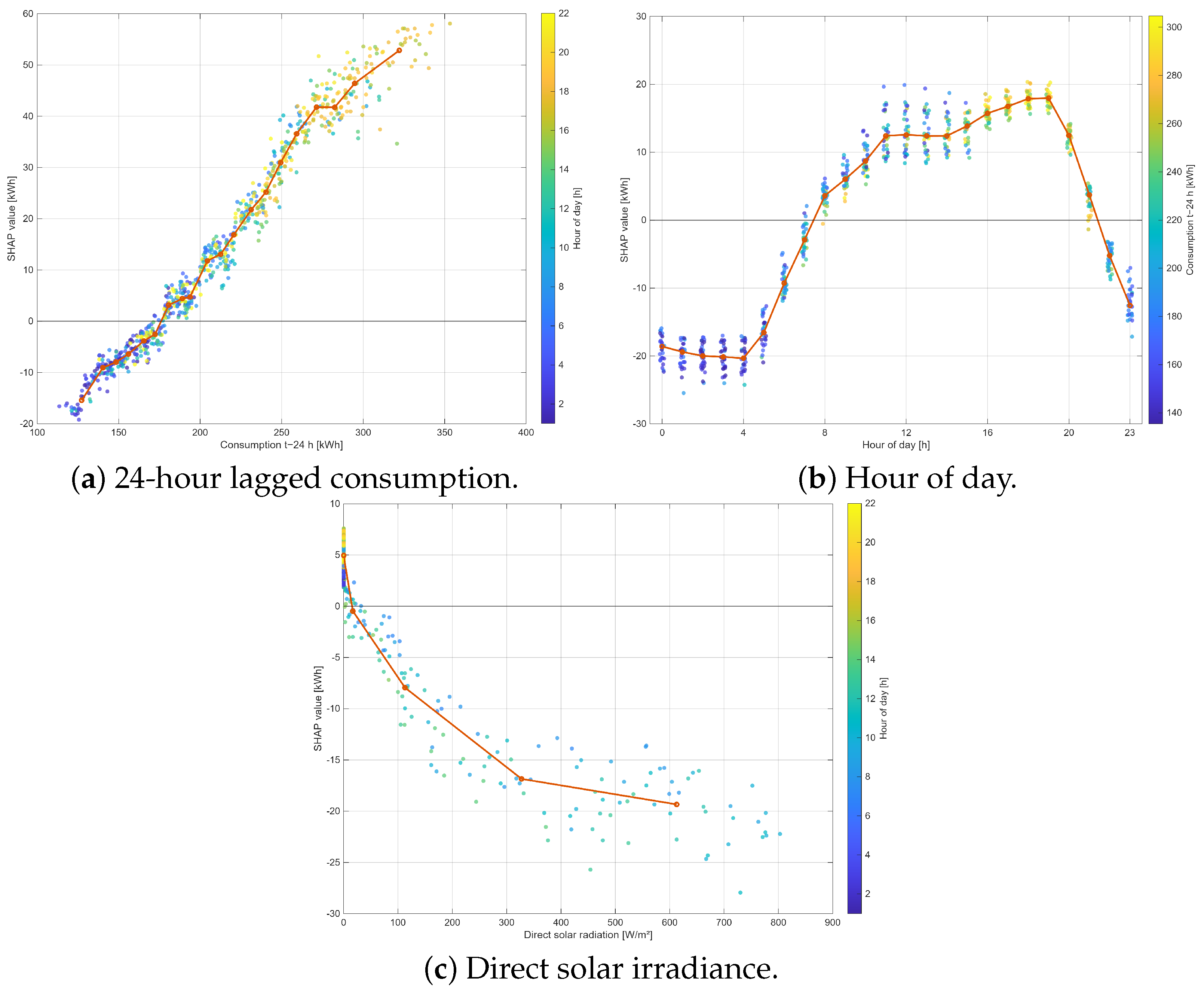
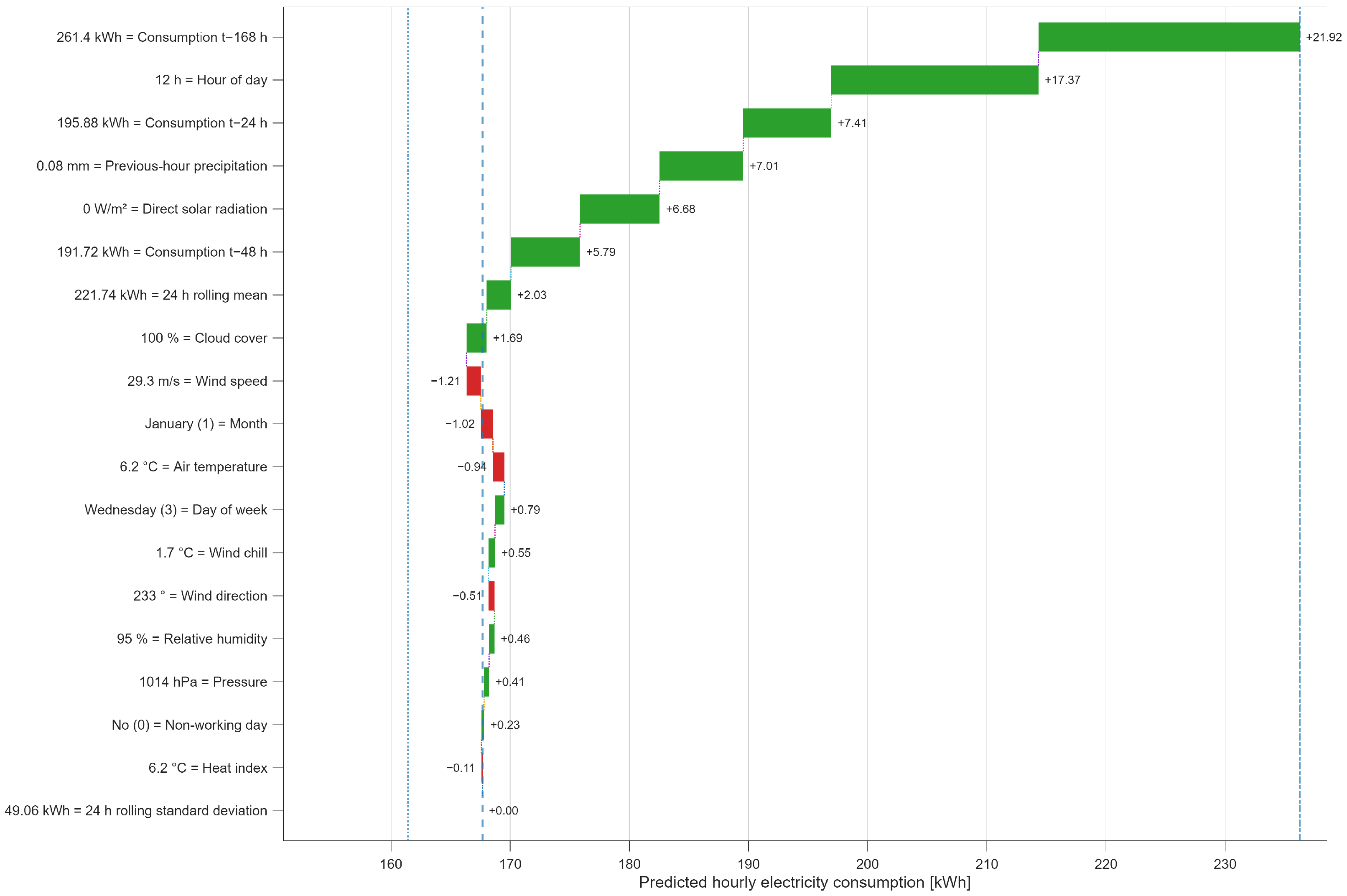
The S1-H1 configuration (winter, sliding, fixed hyperparameters) was retained for detailed beeswarm, waterfall, and SHAP dependence plots as a simple reference configuration combining a 365-day training window with the shared H1 hyperparameters. Before this selection, the complete values of the 19 features and local attributions were verified for all 16 configurations, and a set of control plots was generated. S1-H1 was not selected as the statistically most representative or best-performing configuration. A post hoc quantitative comparison showed, however, that its complete 19-feature SHAP ranking was strongly aligned with the aggregate ranking across all 16 configurations (${\rho }_{\mathrm{s}}=0.9509$). The choice of S1-H1 serves the local diagnostic presentation and does not imply that its local patterns are identical in the remaining configurations.

2.5. Training, Validation, and Testing Procedure

A walk-forward retraining scheme was applied: before each forecasted day, the model was retrained on the current data window.

Each configuration comprises a 31-day test period and its own training window: 365 days for sliding, or all complete rows from 8 January 2023 for expanding. The external evaluation consists of 31 consecutive day-ahead forecasts of 24 h each; no additional holdout test set was set aside.

Let $\mathcal{M}$ denote a single global XGBoost model defined in Section 2.3. For each configuration, the walk-forward retraining proceeds according to the following procedure: (1) the model $\mathcal{M}$ is trained on observations from the initial training window of the given configuration, covering all hours of the day; (2) the model generates forecasts for the 24 h of the first test day; (3) once the actual consumption values for this day become available, these values—rather than the forecasted values—are appended to the training set; (4) the extent of the training window is updated in line with the window strategy (described below); and (5) before forecasting the next day, the model $\mathcal{M}$ is refit on the updated window, with hyperparameters frozen for the entire simulation. Each configuration comprises 31 used model fits: one initial fit and 30 retrainings preceding the forecasts of days 2–31. This yields 31 daily forecasts, i.e., 744 hourly forecasts per configuration. Hyperparameters are not retuned during the loop: in the H1 strategy they come from a single tuning on the shared reference window, and in the H2 strategy from a single tuning on the training window of the given configuration, performed before the start of the simulation (Section 2.3 and Section 2.4).

In expanding, the start of 8 January 2023 remains fixed, while in sliding, after a day is added, the 24 oldest records are removed, keeping the window at 365 days. Both strategies use exclusively data preceding the forecasted day (Figure 2).

In total, 496 used XGBoost fits were performed (16 configurations × 31 days) and nine tuning procedures: one for H1 and eight for H2. To assess sensitivity to algorithmic randomness, an additional fixed-hyperparameter multi-seed analysis was performed using ten predefined random-state values, 38–47, including the original value of 42. The hyperparameters selected in the original H1 and H2 procedures were held fixed at the values reported in Section 3.1, and the Grid Search procedures were not repeated. Thus, this analysis isolates variability associated with stochastic model fitting conditional on the originally selected hyperparameters and does not assess possible random-seed sensitivity of the hyperparameter-selection stage. The same training windows, test periods, feature set, and 31-day walk-forward procedure were retained.

Seven configurations used stochastic observation or feature sampling because either subsample or colsample_bytree was below 1.0. For these configurations, the complete walk-forward procedure was evaluated for all ten random states. In the remaining nine configurations, both sampling parameters were equal to 1.0 and changing the random state did not alter the fitted-model outputs under the fixed parameterization; these configurations therefore served as seed-invariant references. For each realization, MAE, RMSE, and MAPE were recalculated, and between-seed variability was summarized using the mean, standard deviation, and range.

2.6. Forecasting Accuracy Metrics

Accuracy was assessed using MAE (mean absolute error), RMSE (root mean square error), and MAPE (mean absolute percentage error), extending the set of measures used in our previous study [8].

To provide a model-free reference for the reported XGBoost accuracy, two persistence benchmarks were evaluated on exactly the same four 31-day test periods. The 24 h persistence forecast was defined as ${\widehat{y}}_t^{\left(24\right)}=y_{t-24}$ and the 168 h persistence forecast as ${\widehat{y}}_t^{\left(168\right)}=y_{t-168}$. Both forecasts use only consumption values available before the forecasted day, require no model fitting or parameter estimation, and were evaluated using the same MAE, RMSE, and MAPE definitions as the XGBoost forecasts. Because the persistence forecasts depend only on the test period, one set of metrics for each benchmark was computed per seasonal period and used as the reference for the four XGBoost configurations evaluated on that period.

For n observations from the test set, where $y_i$ denotes the actual value of hourly electricity consumption [kWh] and ${\widehat{y}}_i$ the value forecasted by the model [kWh], the metrics are defined as follows:

$$\begin{array}{cc}\hfill \mathrm{MAE}& ={\displaystyle \frac{1}{n}}{\displaystyle \sum _{i=1}^n}\left|y_i-{\widehat{y}}_i\right|,\hfill \end{array}$$

(2)

$$\begin{array}{cc}\hfill \mathrm{RMSE}& =\sqrt{{\displaystyle \frac{1}{n}}\sum _{i=1}^n{\left(y_i-{\widehat{y}}_i\right)}^2},\hfill \end{array}$$

(3)

$$\begin{array}{cc}\hfill \mathrm{MAPE}& ={\displaystyle \frac{1}{n}}{\displaystyle \sum _{i=1}^n}\left|{\displaystyle \frac{y_i-{\widehat{y}}_i}{y_i}}\right|\times 100\%.\hfill \end{array}$$

(4)

MAE and RMSE are expressed in kWh, with RMSE penalizing large deviations more strongly, whereas MAPE describes the relative error. The metrics were reported for full periods and, as auxiliary information, for the a priori fixed peak hours 07:00–10:00 and 17:00–20:00 and for off-peak hours.

The aggregate MAE, RMSE, and MAPE values allow the configurations to be ranked by accuracy but do not resolve whether an observed difference between two configurations is statistically distinguishable. To formally compare the predictive ability of pairs of configurations, a two-sided Diebold–Mariano (DM) test [37] was used, which tests the hypothesis of equal accuracy of two forecasts of the same quantity on the same test set.

The unit of comparison was the complete 24 h profile forecasted from a single daily forecast origin. For configuration m and test day d, the daily absolute loss was defined as

$$L_{m,d}={\displaystyle \frac{1}{24}}{\displaystyle \sum _{r=1}^{24}}\left|y_{d,r}-{\widehat{y}}_{m,d,r}\right|,$$

(5)

where r denotes the position of the hour in the forecasted profile. For two configurations A and B, the series of loss differentials took the form

$$d_d=L_{A,d}-L_{B,d},d=1,\dots ,31.$$

(6)

This formulation preserves the 31 actual forecast origins and does not treat the 744 observations belonging to different hourly horizons as a homogeneous series of forecasts at a 24 h horizon. The null hypothesis is $H_0:\mathbb{E}\left[d_d\right]=0$, and the alternative hypothesis is $H_1:\mathbb{E}\left[d_d\right]\ne 0$. A positive value of the mean loss differential indicates a lower error for configuration B, and a negative value—for configuration A.

In the baseline analysis, $n=31$ non-overlapping daily forecast origins were adopted, with $h=1$ at the scale of successive day-ahead profiles. The statistic was computed as

$$\mathrm{DM}={\displaystyle \frac{\overline{d}}{\sqrt{{\widehat{\gamma }}_0/n}}},\overline{d}={\displaystyle \frac{1}{n}}{\displaystyle \sum _{d=1}^n}{d}_d,$$

(7)

where ${\widehat{\gamma }}_0$ denotes the variance of the series of daily loss differentials estimated with divisor n. For lags $k>0$, the autocovariance was computed as ${\widehat{\gamma }}_k=n^{-1}{\sum }_{d=k+1}^n(d_d-\overline{d})(d_{d-k}-\overline{d})$.

Due to the finite sample size, the Harvey–Leybourne–Newbold (HLN) correction was applied [38]:

$${\mathrm{DM}}^{\ast }=\mathrm{DM}\sqrt{{\displaystyle \frac{n+1-2h+n^{-1}h(h-1)}{n}}},$$

(8)

and the value ${\mathrm{DM}}^{\ast }$ was referred to a Student’s t distribution with $n-1=30$ degrees of freedom. A significance level of $\alpha =0.05$ was adopted. As a sensitivity analysis with respect to possible autocorrelation between consecutive daily losses, a heteroskedasticity- and autocorrelation-consistent (HAC) long-run variance estimator with Bartlett weights was additionally used,

$$\widehat{\mathrm{\Omega }}={\widehat{\gamma }}_0+2{\displaystyle \sum _{k=1}^L}\left(1-{\displaystyle \frac{k}{L+1}}\right){\widehat{\gamma }}_k,$$

(9)

replacing ${\widehat{\gamma }}_0$ in the denominator of Equation (7) with $\widehat{\mathrm{\Omega }}$. The maximum lag was determined deterministically by the rule $L=\lfloor 4{(n/100)}^{2/9}\rfloor =3$. The HAC analysis did not replace the baseline result but served to assess whether the conclusion of significance depends on the way the variance is estimated.

The DM test was applied only to pairs of 31 daily profiles corresponding to the same dates, hours, and actual values. Two families of comparisons were defined: eight sliding–expanding pairs at a fixed season and tuning strategy, and eight H1–H2 pairs at a fixed season and window strategy. For each family of eight tests, a sequential Holm step-down correction was applied separately to control the family-wise error rate. Both the raw p-values and the corrected values were reported, but the main conclusions were based on the $p_{\mathrm{Holm}}$ values from the baseline analysis. Cross-season comparisons cover different test periods and different actual values, and are therefore presented only descriptively, without a paired DM test.

To complement the hypothesis-test results with the magnitude and uncertainty of the paired differences, the mean daily loss differential $\overline{d}$ was additionally reported together with its two-sided 95% confidence interval and the standardized paired effect size Cohen’s $d_z$. The confidence interval was calculated as $\overline{d}\pm t_{0.975,n-1}{s}_d/\sqrt{n}$, where $s_d$ is the sample standard deviation of the 31 paired daily loss differentials. Cohen’s $d_z$ was calculated as $\overline{d}/s_d$. Consistently with the DM definition above, positive values of $\overline{d}$ and $d_z$ indicate lower daily loss for configuration B. The reported confidence intervals are pairwise intervals and are not adjusted for multiple comparisons; family-wise inferential conclusions therefore continue to be based on the Holm-adjusted p-values from the baseline DM-HLN analysis, with the HAC variant used as a sensitivity analysis.

2.7. Model Interpretability Analysis Using SHAP

The SHAP value ${\varphi }_j$ specifies the additive contribution of feature j to the prediction for observation $\mathbf{x}$ [23]:

$${\varphi }_j(f,\mathbf{x})=\sum _{S\subseteq F\setminus \left\{j\right\}}{\displaystyle \frac{\left|S\right|!\left(\right|F|-|S|-1)!}{\left|F\right|!}}\left[v_{\mathbf{x}}\left(S\cup \left\{j\right\}\right)-v_{\mathbf{x}}\left(S\right)\right],$$

(10)

where F denotes the full set of input features, S is a subset of features not containing feature j, and $v_{\mathbf{x}}\left(S\right)$ represents the expected value of the model prediction given the features in the subset S. SHAP values satisfy the property of local additivity:

$$f\left(\mathbf{x}\right)={\varphi }_0+{\displaystyle \sum _{j=1}^p}{\varphi }_j(f,\mathbf{x}),$$

(11)

where ${\varphi }_0$ is the base value of the prediction and p denotes the number of input features. A positive value of ${\varphi }_j$ means that the given feature increases the forecast relative to the base value, whereas a negative value indicates its lowering effect on the forecasted electricity consumption.

For XGBoost, TreeSHAP was applied [24], and both global and local analyses were carried out [20,25,29]. The recovered implementation confirmed that the local attributions were calculated through the native XGBoost prediction interface using pred_contribs=True. Consequently, no separate shap package, feature_perturbation setting, or reference/background dataset was used in this implementation.

The reproducibility of the analysis was considered at two levels. The retained full matrices comprise, for each of the 16 configurations, 744 observations, values of 19 features, 19 local attributions, the forecast, and the base value. They enable independent recomputation of the global rankings, stability statistics, tables, and plots, as well as verification of the additivity equation, without rerunning the models. Together with the recovered training code, these artifacts also enabled the additional multi-seed sensitivity analysis. The serialized models from the original experiment were not retained.

The SHAP analysis was carried out separately for each of the 16 experimental configurations defined in Section 2.4. Due to the applied walk-forward retraining, each configuration comprises 31 successive models, each of which generates a forecast for one test day. SHAP values for each observation were therefore computed using the same daily model that was used to generate the corresponding forecast. This ensures consistency of the explanation with the prediction structure of the model actually used on a given day, rather than interpreting a single model chosen after the experiment. For day d, the corresponding base value ${\varphi }_0^{\left(d\right)}$ applied, constant for the 24 forecasts of that day. Based on the retained results, the additivity of the explanations was confirmed: the sum of ${\varphi }_0^{\left(d\right)}$ and the 19 local attributions reproduced the forecast ${\widehat{y}}_{d,h}$ to a precision limited by the numerical rounding error.

For configuration $v\in \mathcal{V}$, where $\left|\mathcal{V}\right|=16$, the global importance of feature j was determined as the mean absolute SHAP value computed for all observations of its 31-day test set:

$$I_j^{\left(v\right)}={\displaystyle \frac{1}{n_v}}{\displaystyle \sum _{i=1}^{n_v}}\left|{\varphi }_{j,i}^{\left(v\right)}\right|,$$

(12)

where $n_v=744$ denotes the number of hourly forecasts in a given configuration, and ${\varphi }_{j,i}^{\left(v\right)}$ is the SHAP value of feature j for observation i, computed using the model in effect on the forecast day. The measure $I_j^{\left(v\right)}$ is expressed in the units of the forecasted variable, i.e., in kWh, and describes the average absolute change in the prediction attributed to the analyzed feature in a given configuration.

Because the overall scale of SHAP values may differ between seasons and model configurations, for the purpose of comparing all configurations, normalization was applied within each configuration:

$$W_j^{\left(v\right)}={\displaystyle \frac{I_j^{\left(v\right)}}{{\displaystyle {\displaystyle \sum _{k=1}^p}{I}_k^{\left(v\right)}}}},{\displaystyle \sum _{j=1}^p}{W}_j^{\left(v\right)}=1.$$

(13)

The value $W_j^{\left(v\right)}$ represents the relative contribution of feature j to the total global importance of all features in configuration v. The normalization serves exclusively for comparing the structure of importance between configurations; the interpretation of the magnitude of the contribution in physical units was based on the unnormalized values $I_j^{\left(v\right)}$. Because the normalized shares are compositional, a change in $W_j^{\left(v\right)}$ may reflect either a change in $I_j^{\left(v\right)}$ itself or a redistribution caused by changes in the absolute SHAP magnitudes of the remaining features; normalized and absolute importance are therefore interpreted jointly.

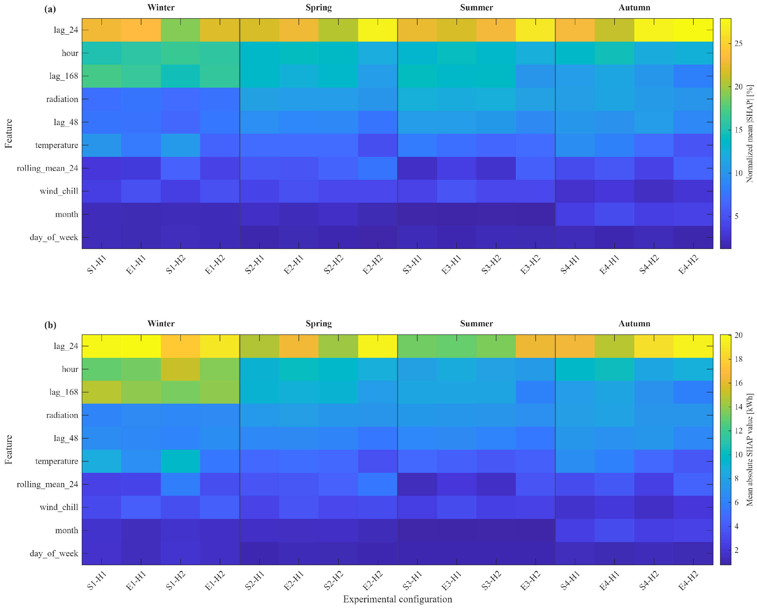
The normalized values are presented as a joint heatmap whose columns correspond to the 16 experimental configurations and whose rows correspond to the ten features with the highest average importance across the entire experiment. The average importance aggregating the results from all configurations was defined as

$${\overline{W}}_j={\displaystyle \frac{1}{\left|\mathcal{V}\right|}}\sum _{v\in \mathcal{V}}{W}_j^{\left(v\right)}.$$

(14)

The features were ordered in decreasing order of ${\overline{W}}_j$, and the ten highest-ranked variables were selected for the heatmap. This approach makes it possible to simultaneously assess the dominant predictors and the changes in their relative importance between seasons, training-window strategies, and hyperparameter tuning strategies, without presenting 16 separate importance plots.

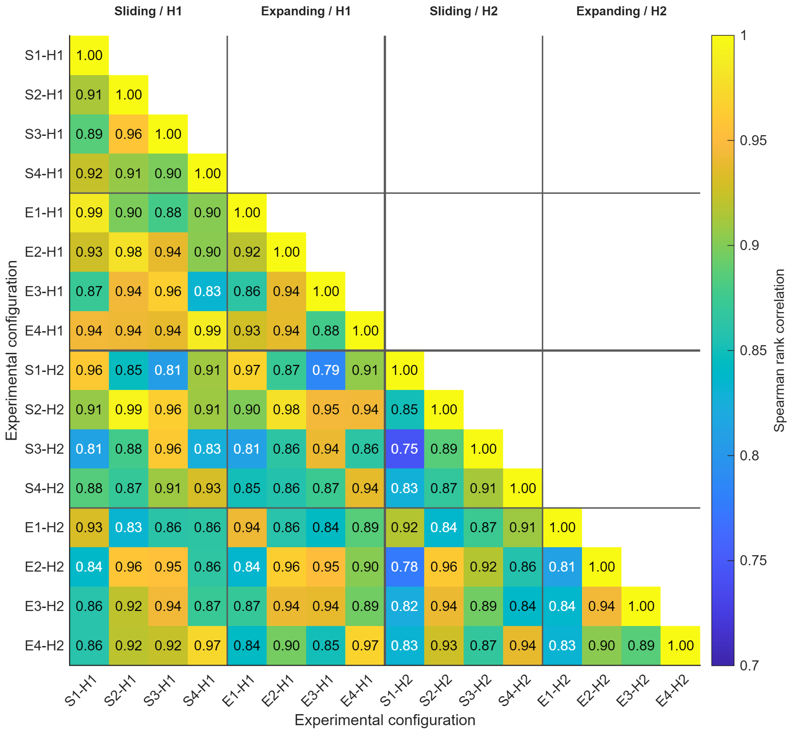
The stability of model interpretation was evaluated based on the agreement of feature rankings between configurations. For each configuration, a rank vector ${\mathbf{R}}^{\left(v\right)}$ was constructed, covering all $p=19$ features ordered in decreasing order of $I_j^{\left(v\right)}$. The agreement of two rankings, corresponding to configurations a and b, was determined using the Spearman rank correlation coefficient:

$${\rho }_{\mathrm{s}}^{(a,b)}=corr\left({\mathbf{R}}^{\left(a\right)},{\mathbf{R}}^{\left(b\right)}\right).$$

(15)

A value of ${\rho }_{\mathrm{s}}$ close to 1 indicates high ranking agreement, a value close to 0 indicates the absence of monotonic agreement, and a negative value indicates opposite feature orderings. No discrete threshold classifying a ranking as stable or unstable was adopted in the study; the interpretation was based on the continuous values of the coefficient and their comparison between groups of configurations. The correlation was computed for the full set of 19 features rather than only for the variables shown in the heatmap, in order to limit the influence of an arbitrary feature-selection threshold on the assessment of agreement. To complement Spearman’s coefficient with a measure focused on the most influential predictors, pairwise Top-5 overlap was calculated as $O_5^{(a,b)}=|{\mathcal{T}}_5^{\left(a\right)}\cap {\mathcal{T}}_5^{\left(b\right)}|/5$, where ${\mathcal{T}}_5^{\left(v\right)}$ denotes the set of the five highest-ranked features in configuration v. Thus, $O_5=1$ denotes identical Top-5 feature sets, irrespective of their internal ordering.

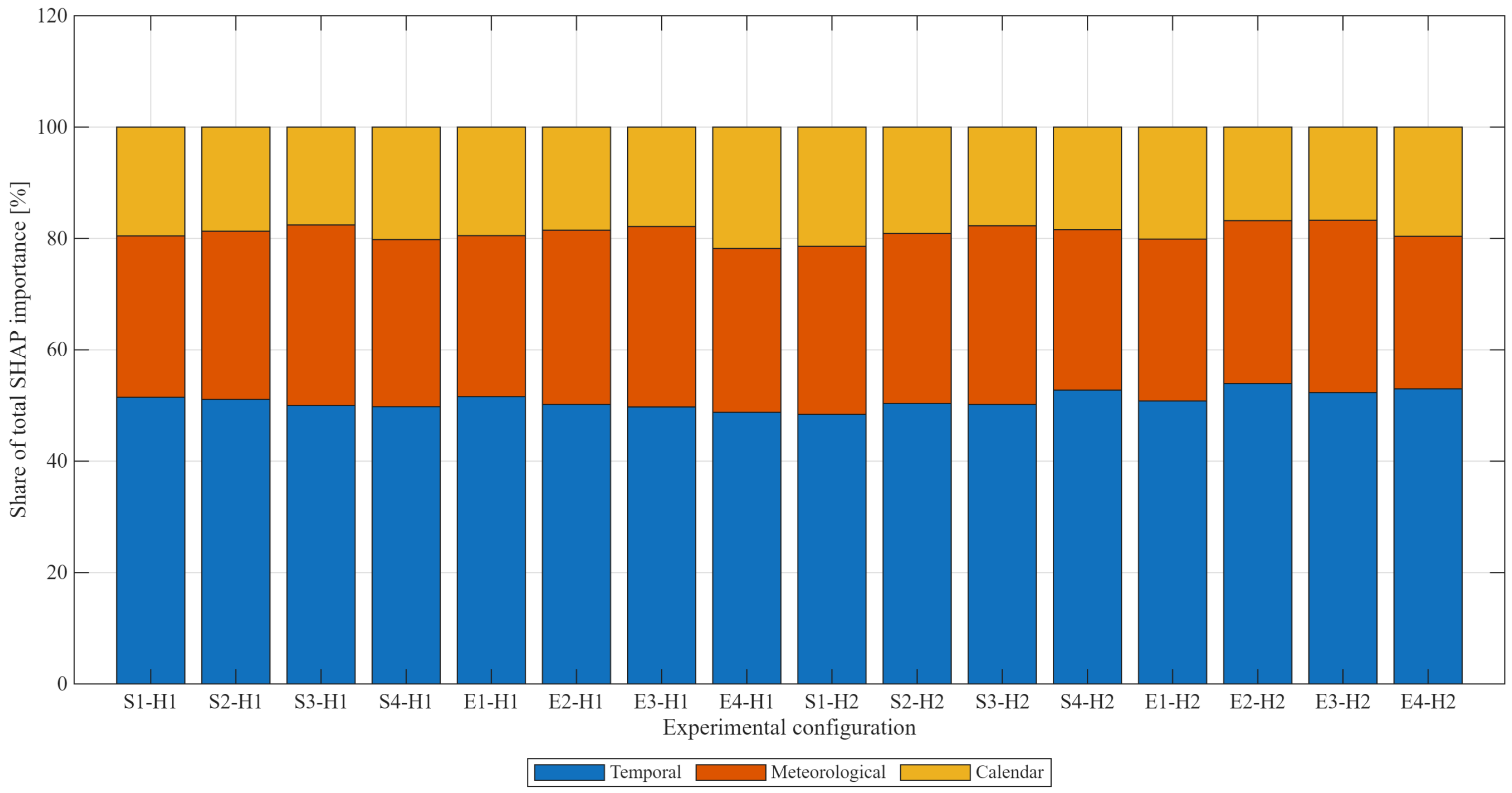
In this study, the term stability denotes the descriptive agreement of rankings generated by the same TreeSHAP procedure for the analyzed models. It should not be equated with unambiguous identification of a physical mechanism or with the invariance of individual attributions in the presence of collinear predictors. In particular, features describing related phenomena, such as temperature-related variables and load lags and rolling statistics, may share or take over part of the attributed contribution depending on the structure of the trained trees. For this reason, conclusions concerning groups of features are more robust than fine differences in the ranking position of individual variables.

The stability analysis was carried out in two stages. In the first stage, the full matrix of Spearman coefficients was computed for all 16 configurations, comprising 120 unique pairs. In the second stage, 40 targeted comparisons were extracted, corresponding to the three dimensions of the experiment:

1.

Stability with respect to season—All pairs of the four seasons were compared separately in each of the four configuration families: sliding–H1, expanding–H1, sliding–H2, and expanding–H2. In each family, six comparisons were performed, yielding a total of 24 cross-season pairs. In the H1 families the actual hyperparameters remain fixed, whereas in the H2 families they could differ between seasons as a result of independent tuning; therefore the H2 results describe the stability of rankings between complete seasonal configurations rather than the isolated effect of the season itself. In contrast to the Diebold–Mariano test (Section 2.6), the rank correlation can also be computed for rankings coming from different test periods.

2.

Stability with respect to the training-window strategy—For each season, sliding and expanding were compared separately for H1 and H2, yielding a total of eight pairs. For H1, the comparison keeps the actual hyperparameters fixed and allows the cleanest assessment of the change associated with the window strategy. For H2, both configurations belong to the same tuning strategy, but their selected hyperparameters could differ; the comparison therefore has the character of a descriptive assessment of the stability of complete configurations.

3.

Stability with respect to the hyperparameter tuning strategy—for each season and window type, the corresponding H1 and H2 configurations were compared: four pairs for sliding and four for expanding, eight comparisons in total.

For the full matrix, the mean, median, and range of the coefficients were reported, whereas for the 40 targeted comparisons, analogous statistics were determined separately for the three groups. The distinction between comparisons that isolate a single factor and comparisons of full configurations reduces the risk of attributing observed changes exclusively to one element of the procedure, when in the H2 configurations the actual sets of hyperparameters could differ.

Algorithmic-randomness sensitivity was evaluated separately from the across-configuration stability analysis. For each random state, global mean absolute SHAP importance and the ranking of all 19 features were recomputed. Within each stochastic configuration, the ten seed-specific rankings yielded 45 unique seed-to-seed pairs, for which Spearman’s rank correlation was calculated. Agreement among the most influential predictors was additionally checked through the overlap of the five highest-ranked features. Finally, the complete set of 120 across-configuration Spearman coefficients was recalculated separately for each random state to determine whether the main ranking-agreement result depended materially on the stochastic realization.

Uncertainty in global SHAP importance and feature rankings was additionally evaluated using a day-level block bootstrap. For each configuration, the 744 local SHAP observations were divided into the 31 complete 24 h forecast-day blocks generated by the successive daily models. A total of 10,000 bootstrap samples were generated by resampling these daily blocks with replacement. For each replicate, mean absolute SHAP importance in kWh, normalized SHAP shares, and the complete ranking of all 19 features were recalculated. The 2.5th and 97.5th percentiles of the bootstrap distribution were used as 95% percentile confidence limits for mean absolute SHAP importance. Ranking uncertainty was evaluated using Spearman correlation between each bootstrap ranking and the corresponding original ranking and by the overlap of the five highest-ranked features. For summaries averaged across the 16 configurations, the same resampled day indices were applied to the four configurations sharing a given seasonal test period, preserving their paired day structure. The bootstrap therefore quantifies uncertainty conditional on the four observed 31-day test periods and does not constitute replication across independent years or seasonal windows.

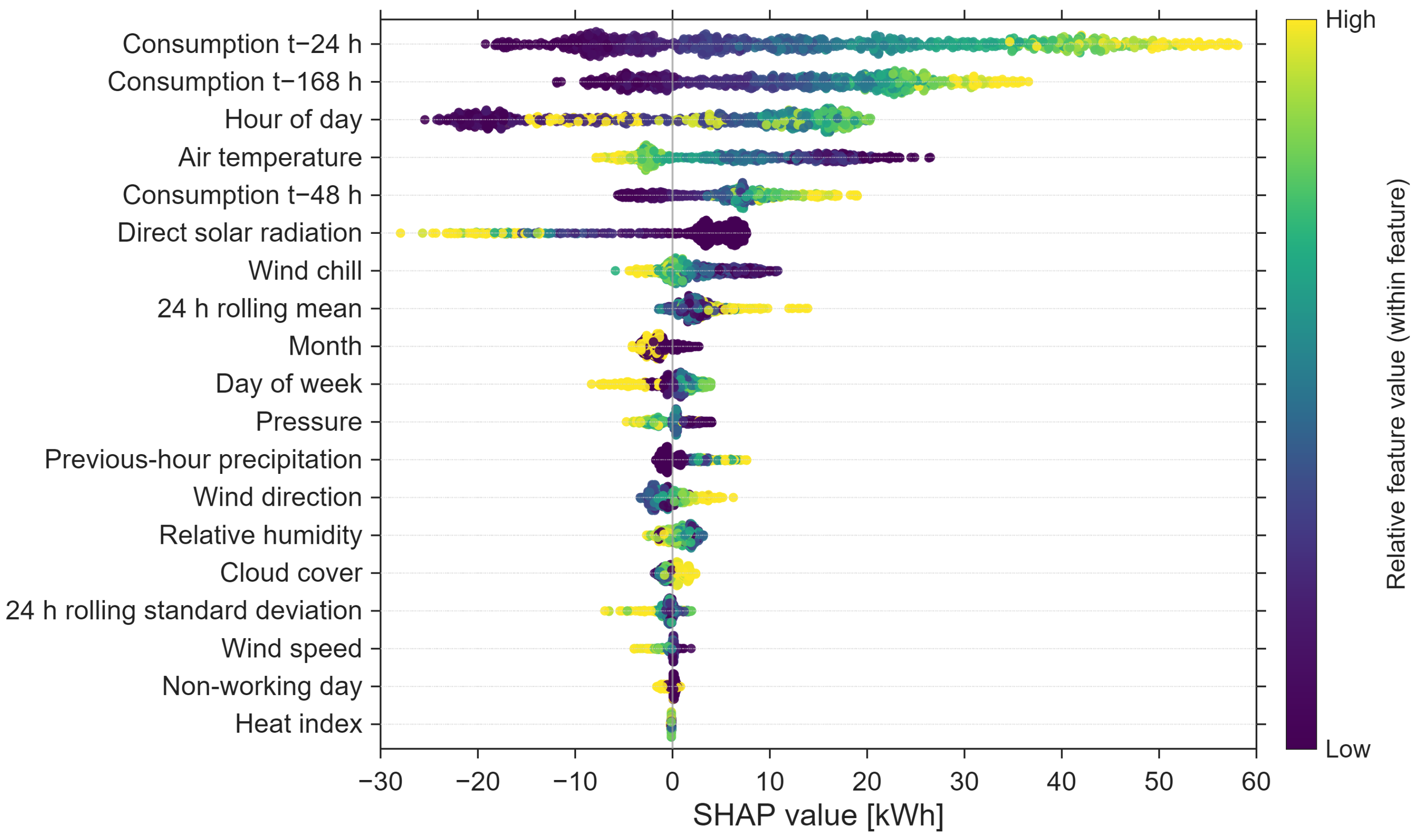
For each configuration, a matrix of 744 forecasts, actual values, base values, 19 feature values, and 19 attributions was prepared. The inspection confirmed the completeness of the data and a maximum additivity error below 0.001 kWh. The detailed local presentation was restricted to the reference S1-H1, whose feature hierarchy was consistent with the global result. The beeswarm plots show the distribution of attributions, and the dependence plots—their nonlinear direction without a causal interpretation [34]. Two local cases from the S1-H1 configuration were selected explicitly by absolute-error criterion: the case with absolute error closest to the median was retained as a numerical reference, whereas the case with the maximum absolute error was presented on a waterfall plot for detailed diagnostic inspection.

The SHAP analysis was purely post hoc in nature. Its results were not used for feature selection, hyperparameter tuning, or modifying the models evaluated on the test sets, so that the interpretation did not influence the results of the accuracy comparison of individual configurations.

2.8. Use of Generative AI-Assisted Tools

During the preparation and revision of the manuscript, OpenAI ChatGPT (GPT-5.6 Sol; accessed in July–August 2026) was used as an assisting tool. It supported translation from Polish into English and the technical implementation in TikZ of the author-developed designs of Figure 1 and Figure 2. The conceptual content, structure, and graphical layout of these figures were developed by the authors; ChatGPT was used only to convert the author-developed designs into TikZ source code. ChatGPT was also used to assist with the preparation of reproducibility scripts and the checking of selected additional calculations introduced in response to the reviewers. The corresponding additional analyses and results are reported in Section 2 and Section 3, including Section 3.3 and Tables. The methodological design, execution of the calculations, evaluation of the resulting outputs, and their interpretation were performed by the authors. For the AI-assisted reproducibility scripts and selected additional calculations, the resulting numerical outputs were checked by the authors against the retained forecast and SHAP matrices, where applicable, and through the numerical consistency checks described in the relevant methodological subsections. All AI-assisted material used in the manuscript was reviewed and edited by the authors, who take full responsibility for the content of this publication.

3. Results

3.1. Hyperparameter Selection and Overall Forecasting Performance

Nine grid searches of 216 combinations with five TimeSeriesSplit folds were performed: one for the shared H1 strategy and eight for H2. The selected parameters were frozen for the 31-day simulation and are listed in

Table 6. Selected XGBoost hyperparameters and mean validation MAE. H1 denotes the shared configuration for all corresponding configurations; H2 validation MAE values obtained from different windows do not constitute a ranking of test results.

Configuration	n_estimators	max_depth	learning_rate	subsample	colsample_bytree	gamma	${\mathbf{MAE}}_{\mathbf{CV}}$ [kWh]
H1 (S1-H1–E4-H1)	500	3	0.05	1.0	1.0	0.0	14.58
S1-H2	500	3	0.10	0.8	1.0	0.0	14.39
S2-H2	300	3	0.10	0.8	1.0	0.0	15.45
S3-H2	500	3	0.05	1.0	0.8	0.5	16.32
S4-H2	300	3	0.05	0.8	0.8	0.0	13.12
E1-H2	300	3	0.10	1.0	0.8	0.0	14.60
E2-H2	300	5	0.05	1.0	0.8	0.5	14.29
E3-H2	500	5	0.05	1.0	1.0	0.0	13.99
E4-H2	300	5	0.05	0.8	0.8	0.0	12.04

.

H1 selected 500 trees, depth 3, and learning_rate=0.05. H2 produced different configurations, confirming that the validation optimum depended on the training window. Ties for H1, E1-H2, and S4-H2 were resolved deterministically by the grid order. Because the H2 validation MAE values came from different windows, they were not used to rank the test configurations.

Each grid search involved 1080 validation fits. H1 therefore required 1080 fits and H2 required 8640, an eightfold increase in tuning cost. This ratio excludes the 248 daily final fits performed in each strategy group. The walk-forward fitting and inference workload was equal in count for the two strategy groups: each comprised 248 final model fits and generated 5952 hourly forecasts. Comparable measurements of total runtime, daily refitting time, and inference time were not retained. Consequently, the computational comparison is reported in reproducible fit counts rather than wall-clock time.

Table 7. Day-ahead forecast accuracy for the 16 experimental configurations (full test period, 744 h). The best value of each metric is shown in bold.

Configuration	MAE [kWh]	RMSE [kWh]	MAPE [%]
S1-H1	13.94	18.59	7.03
S2-H1	11.39	15.22	8.64
S3-H1	8.05	10.60	6.15
S4-H1	14.89	20.84	8.64
E1-H1	14.21	19.00	7.24
E2-H1	10.87	14.40	8.30
E3-H1	8.25	10.74	6.31
E4-H1	14.69	20.66	8.40
S1-H2	13.93	18.63	6.99
S2-H2	11.34	15.14	8.59
S3-H2	8.07	10.59	6.17
S4-H2	14.98	21.27	8.64
E1-H2	14.01	18.77	7.13
E2-H2	10.79	14.23	8.22
E3-H2	7.79	10.25	6.01
E4-H2	13.76	19.29	7.90

summarizes day-ahead accuracy for the 16 configurations over their full 31-day test periods (744 hourly forecasts each).

MAE ranged from 7.79 to 14.98 kWh, RMSE from 10.25 to 21.27 kWh, and MAPE from 6.01 to 8.64%. E3-H2 achieved the lowest value of all three metrics. The largest descriptive variation occurred between the selected seasonal test periods, while differences associated with the window and tuning strategies were smaller and configuration-dependent.

To place the XGBoost results in a direct model-free context, the same four 31-day test periods were also evaluated using 24 h and 168 h persistence forecasts.

Table 8. Accuracy of the 24 h and 168 h persistence benchmarks over the four 31-day test periods (744 h each).

Test Period	24 h Persistence			168 h Persistence
	MAE [kWh]	RMSE [kWh]	MAPE [%]	MAE [kWh]	RMSE [kWh]	MAPE [%]
Winter	20.80	29.12	10.51	29.83	38.82	15.28
Spring	15.38	22.07	11.58	27.64	36.91	21.62
Summer	11.41	15.67	8.78	12.14	16.41	9.36
Autumn	17.73	25.02	10.49	27.17	37.16	15.13

summarizes the resulting MAE, RMSE, and MAPE values.

The 24 h persistence forecast was more accurate than the 168 h benchmark in all four test periods. Nevertheless, each of the 16 XGBoost configurations in Table 7 achieved lower MAE, RMSE, and MAPE than both persistence benchmarks for the corresponding period. Relative to the stronger 24 h persistence benchmark, the MAE reduction across the 16 XGBoost configurations ranged from 15.5% to 33.0%. These results provide a descriptive external reference for the forecasting accuracy of the evaluated XGBoost configurations.

3.2. Forecast Accuracy Across Experimental Factors and Time

Configurations were compared along the three experimental dimensions. For each pair, the absolute difference was calculated as the metric value for the compared configuration minus that for the reference configuration, and the relative difference was expressed as a percentage of the reference value. A negative difference therefore denotes a lower error for the compared configuration.

Differences among the four selected seasonal test periods were assessed descriptively. The selected summer test period produced the lowest MAE, RMSE, and MAPE in all four configuration families. Relative to the corresponding summer configuration, MAE was higher by 31.69–41.56% in the selected spring test period, 72.18–79.87% in the selected winter test period, and 76.55–85.61% in the selected autumn test period. MAPE yielded a partially different ordering, especially for the selected winter test period, which supports joint reporting of absolute and relative errors. Formal inference across seasonal test periods would require multiple independent seasonal windows.

The training-window strategies were compared for the same season and tuning strategy. Each metric cell in

Table 9. Comparison of expanding and sliding strategies. Metric cells report the absolute difference followed by the relative difference in parentheses; differences were computed as expanding minus sliding.

Pair	$\mathbf{\Delta }$MAE [kWh (%)]	$\mathbf{\Delta }$RMSE [kWh (%)]	$\mathbf{\Delta }$MAPE [pp (%)]	$\overline{\mathit{d}}$ [kWh] (95% CI)	${\mathit{d}}_{\mathit{z}}$	DM*	${\mathit{p}}_{\mathbf{raw}}/{\mathit{p}}_{\mathbf{Holm}}$
S1-H1–E1-H1	0.27 (1.93)	0.41 (2.23)	0.211 (3.00)	$-0.269$ [$-0.721$, 0.183]	$-0.218$	−1.214	0.2344/0.7032
S2-H1–E2-H1	−0.52 (−4.59)	−0.82 (−5.38)	−0.335 (−3.88)	0.523 [0.052, 0.993]	0.408	2.269	0.0306/0.2142
S3-H1–E3-H1	0.21 (2.56)	0.14 (1.32)	0.151 (2.45)	$-0.206$ [$-0.435$, 0.023]	$-0.330$	−1.838	0.0760/0.4562
S4-H1–E4-H1	−0.20 (−1.31)	−0.18 (−0.87)	−0.236 (−2.73)	0.195 [$-0.320$, 0.711]	0.139	0.774	0.4449/0.8897
S1-H2–E1-H2	0.08 (0.61)	0.14 (0.73)	0.146 (2.09)	$-0.085$ [$-0.650$, 0.481]	$-0.055$	−0.306	0.7618/0.8897
S2-H2–E2-H2	−0.55 (−4.89)	−0.91 (−6.00)	−0.372 (−4.33)	0.554 [$-0.118$, 1.227]	0.302	1.683	0.1028/0.4562
S3-H2–E3-H2	−0.28 (−3.45)	−0.33 (−3.14)	−0.167 (−2.71)	0.278 [$-0.033$, 0.589]	0.328	1.828	0.0775/0.4562
S4-H2–E4-H2	−1.22 (−8.16)	−1.97 (−9.29)	−0.745 (−8.62)	1.222 [0.347, 2.096]	0.512	2.852	0.0078/0.0623

The DM test used 31 daily profiles and $d_d=L_{A,d}-L_{B,d}$; a positive DM* indicates lower daily loss for configuration B. Holm correction was applied within the family of eight tests. The columns $\overline{d}$ and $d_z$ follow the same sign convention; the 95% confidence intervals are pairwise and are not multiplicity-adjusted. In the HAC sensitivity analysis, no comparison reached $p_{\mathrm{Holm},\mathrm{HAC}}<0.05$; the smallest corrected HAC value was 0.0732.

and 

Table 10. Comparison of H2 and H1 strategies. Metric cells report the absolute difference followed by the relative difference in parentheses; differences were computed as H2 minus H1.

Pair	$\mathbf{\Delta }$MAE [kWh (%)]	$\mathbf{\Delta }$RMSE [kWh (%)]	$\mathbf{\Delta }$MAPE [pp (%)]	$\overline{\mathit{d}}$ [kWh] (95% CI)	${\mathit{d}}_{\mathit{z}}$	DM*	${\mathit{p}}_{\mathbf{raw}}/{\mathit{p}}_{\mathbf{Holm}}$
S1-H1–S1-H2	−0.01 (−0.08)	0.04 (0.22)	−0.045 (−0.64)	0.012 [$-0.429$, 0.452]	0.010	0.054	0.9572/1.0000
S2-H1–S2-H2	−0.05 (−0.43)	−0.08 (−0.53)	−0.049 (−0.56)	0.049 [$-0.202$, 0.300]	0.072	0.400	0.6923/1.0000
S3-H1–S3-H2	0.02 (0.28)	−0.01 (−0.12)	0.020 (0.32)	$-0.022$ [$-0.133$, 0.088]	$-0.074$	−0.414	0.6816/1.0000
S4-H1–S4-H2	0.09 (0.59)	0.43 (2.05)	0.004 (0.05)	$-0.089$ [$-0.388$, 0.211]	$-0.109$	−0.604	0.5502/1.0000
E1-H1–E1-H2	−0.20 (−1.38)	−0.24 (−1.25)	−0.110 (−1.52)	0.196 [$-0.202$, 0.593]	0.181	1.005	0.3228/1.0000
E2-H1–E2-H2	−0.08 (−0.74)	−0.17 (−1.19)	−0.085 (−1.03)	0.081 [$-0.317$, 0.478]	0.074	0.415	0.6813/1.0000
E3-H1–E3-H2	−0.46 (−5.59)	−0.49 (−4.52)	−0.298 (−4.73)	0.462 [0.115, 0.808]	0.488	2.719	0.0108/0.0754
E4-H1–E4-H2	−0.94 (−6.38)	−1.37 (−6.62)	−0.505 (−6.01)	0.938 [0.291, 1.585]	0.532	2.959	0.0060/0.0477

The DM test used 31 daily profiles and $d_d=L_{A,d}-L_{B,d}$; a positive DM* indicates lower daily loss for configuration B. Holm correction was applied within the family of eight tests. Bold denotes $p_{\mathrm{Holm}}<0.05$. The columns $\overline{d}$ and $d_z$ follow the same sign convention; the 95% confidence intervals are pairwise and are not multiplicity-adjusted. In the HAC sensitivity analysis, the Holm-adjusted values were 0.0354 for E3-H1–E3-H2 and 0.0357 for E4-H1–E4-H2; no other H1–H2 comparison reached the 0.05 threshold.

reports the absolute difference followed, in parentheses, by the corresponding relative change with respect to configuration A in the pair. For MAE and RMSE, the absolute differences are expressed in kWh; for MAPE, they are expressed in percentage points (pp). Negative values indicate a lower error for configuration B. In Table 9, differences were computed as expanding minus sliding.

The expanding strategy reduced MAE in five of eight comparisons, but the direction depended on the test period. The largest improvement was observed for E4-H2 relative to S4-H2 ($-8.16\%$). For this comparison, the mean paired daily-loss difference was 1.222 kWh (95% CI: 0.347–2.096 kWh; $d_z=0.512$). The pairwise confidence interval also excluded zero for S2-H1–E2-H1 ($\overline{d}=0.523$ kWh, 95% CI: 0.052–0.993 kWh; $d_z=0.408$). These intervals are not adjusted for multiple comparisons and therefore do not by themselves constitute family-wise evidence of superiority. After Holm correction, no sliding–expanding pair was statistically distinguishable ($p_{\mathrm{Holm}}\ge 0.0623$), and the HAC sensitivity analysis did not alter this conclusion ($p_{\mathrm{Holm},\mathrm{HAC}}\ge 0.0732$).

The tuning strategies were compared for the same season and training-window type. In Table 10, differences were computed as H2 minus H1.

H2 reduced MAE in six of eight pairs, with the largest improvements for E4 ($-6.38\%$) and E3 ($-5.59\%$). The corresponding paired daily-loss effects were $\overline{d}=0.938$ kWh (95% CI: 0.291–1.585 kWh; $d_z=0.532$) for E4 and $\overline{d}=0.462$ kWh (95% CI: 0.115–0.808 kWh; $d_z=0.488$) for E3. The pairwise confidence intervals for the remaining six H1–H2 comparisons included zero. After Holm correction, the baseline analysis supported H2 only for E4 ($p_{\mathrm{Holm}}=0.0477$); the E3 result was not significant in the baseline ($p_{\mathrm{Holm}}=0.0754$) but became significant in the HAC variant ($p_{\mathrm{Holm},\mathrm{HAC}}=0.0354$; for E4, $p_{\mathrm{Holm},\mathrm{HAC}}=0.0357$). The E3 result should therefore be regarded as variance-estimator dependent rather than robustly significant.

Temporal error variation was evaluated for fixed peak and off-peak hours, by hour of day, and across the successive test days. The analysis covered all 11,904 hourly forecasts. The peak period comprised 248 observations per configuration (07:00–10:00 and 17:00–20:00), and the remaining 496 observations were classified as off-peak.

MAE was larger during peak hours in 11 of 16 configurations, whereas MAPE was smaller in 13. Mean peak and off-peak MAE values were 12.48 and 11.66 kWh, respectively, while the corresponding MAPE values were 7.05% and 7.76%. Thus, conclusions about the more difficult period depended on whether error was expressed in absolute or relative terms.

For each hour, MAE was calculated from 31 observations per configuration. Figure 3 shows the hourly profiles averaged across the four configurations representing each season.

Across all configurations, hourly MAE was lowest at 3:00 (7.37 kWh) and highest at 14:00 (17.79 kWh), with values of 15.00–17.79 kWh between 10:00 and 16:00. The hour of maximum seasonal MAE was 14:00 in winter, 16:00 in spring and summer, and 12:00 in autumn; the corresponding values were 23.61, 15.72, 14.13, and 25.20 kWh. The minimum occurred at 0:00 in winter, 3:00 in spring and summer, and 1:00 in autumn.

Hourly MAPE showed a similar profile, with a maximum of 10.82% at 14:00 and a minimum of 4.82% at 19:00. The overall mean signed error was 0.11 kWh. The largest mean overestimation occurred at 12:00 ($-2.59$ kWh), and the largest mean underestimation at 17:00 (2.86 kWh).

For each of the 496 configuration–day pairs, a separate daily MAE was calculated. Figure 4 presents the metric across the 31 test days, averaged across the four configurations for each season.

Daily MAE for individual configuration–day pairs ranged from 4.34 to 35.24 kWh. The lowest value occurred on 15 May for E2-H2 and the highest on 9 November for S4-H2. Seasonal-average maxima occurred on 18 January, 21 April, 16 July, and 9 November, reaching 23.88, 20.36, 10.48, and 33.82 kWh, respectively. Winter and autumn shared the same maximum-error day across all four corresponding configurations. Spring differed in one configuration, whereas each summer configuration reached its maximum on a different day.

The largest APE, 67.25%, occurred on 1 November at 15:00 for S4-H2 and at the same moment in all four autumn configurations. In S4-H2, observed consumption was 118.92 kWh and the forecast was 198.89 kWh. The lag values were 204.90, 205.82, and 192.40 kWh, i.e., 38.19–42.22% above the observation. Across the four autumn models, the three lags contributed +29.48 to +32.20 kWh, whereas day_off reduced the forecast by only 0.94–3.57 kWh. No record error was found. This diagnostic case supports a richer representation of holidays and adjacent days, but does not establish a causal relationship.

3.3. Global SHAP Importance and Ranking Stability

Global importance was calculated from mean absolute SHAP values for all 19 features and normalized within each configuration (Equations (13) and (14)).

Table 11. Ten features with the highest average normalized SHAP importance across the 16 configurations, with the corresponding mean absolute SHAP values and 95% day-level bootstrap confidence intervals. Feature groups: Temporal (T), Meteorological (M), and Calendar (C).

Rank	Feature	Group	Mean $\left|\mathbf{SHAP}\right|$ [kWh] (95% Bootstrap CI)	Mean Share (Range) [%]	Median Rank	Top 3/Top 5
1	lag_24	T	16.70 (15.91–17.54)	23.33 (19.09–27.90)	1.0	16/16
2	hour	C	10.12 (9.94–10.32)	13.95 (12.07–16.51)	2.0	16/16
3	lag_168	T	9.43 (8.97–9.93)	12.95 (8.33–17.15)	3.0	12/16
4	radiation	M	7.13 (6.81–7.44)	10.16 (6.90–12.51)	4.0	3/15
5	lag_48	T	6.42 (6.22–6.64)	9.09 (6.64–10.71)	5.0	1/13
6	temperature	M	5.45 (4.86–6.06)	7.48 (4.88–10.52)	6.0	0/3
7	rolling_mean_24	T	3.44 (3.14–3.76)	4.77 (2.35–7.63)	7.0	0/1
8	wind_chill	M	2.87 (2.61–3.13)	3.99 (2.24–5.29)	8.0	0/0
9	month	C	1.67 (1.55–1.79)	2.31 (1.26–4.61)	10.5	0/0
10	day_of_week	C	1.26 (1.09–1.45)	1.75 (1.41–2.11)	10.0	0/0

Bootstrap confidence intervals are the 2.5th and 97.5th percentiles obtained from 10,000 day-level block-bootstrap replicates. Complete 24 h forecast-day blocks were resampled, preserving the within-day dependence of the local SHAP observations.

summarizes the ten highest-ranked features across the 16 configurations.

lag_24 ranked first in every configuration, with a mean absolute importance of 16.70 kWh and a mean normalized share of 23.33%. The next positions were occupied by hour (10.12 kWh; 13.95%) and lag_168 (9.43 kWh; 12.95%). Direct solar irradiance was the highest-ranked meteorological feature (10.16%) and appeared in the top five in 15 configurations. The subsequent positions were occupied by lag_48 and temperature. The first five features accounted for 69.48% of aggregated importance and the first ten for 89.78%.

The paired heatmaps confirm the dominance of lag_24 and the consistently high positions of hour and lag_168. Configuration-dependent changes were more visible for lag_168, radiation, temperature, rolling_mean_24, and month. Comparison of panels (a) and (b) distinguishes changes in relative importance from changes in absolute attribution magnitude: a change in normalized share does not necessarily imply a corresponding change in mean absolute SHAP value. Descriptively, the leading predictors show larger differences between some of the four seasonal test periods than among the S-H1, E-H1, S-H2, and E-H2 configurations within the same period. These patterns refer to the specific 31-day test periods and should not be interpreted as isolated causal effects of season, training-window strategy, or hyperparameter-selection strategy.

For the six principal predictors, the observed extrema of absolute mean $\left|\mathrm{SHAP}\right|$ further illustrate the configuration-dependent variation shown in Figure 5. For lag_24, the values ranged from 13.08 kWh in E3-H1 to 20.06 kWh in E1-H1; for hour, from 7.50 kWh in E3-H2 to 15.23 kWh in S1-H2; and for lag_168, from 5.85 kWh in E4-H2 to 14.85 kWh in S1-H1. The corresponding ranges were 6.25–8.00 kWh for radiation (S1-H1 to E4-H1), 5.49–7.30 kWh for lag_48 (E2-H2 to S4-H1), and 3.51–9.70 kWh for temperature (E2-H2 to S1-H2). The clearest changes were associated with the selected seasonal test periods: absolute hour and lag_168 attribution was highest in the winter configurations, whereas the normalized contribution of radiation was higher outside the winter period. Temperature attribution was also largest in the winter configurations. In contrast, no monotonic pattern common to the principal predictors was observed for the sliding–expanding or H1–H2 comparisons within the seasonal blocks.

The normalized and absolute panels should not be interpreted interchangeably. For example, the normalized share of lag_24 ranged from 19.09% in S1-H2 to 27.90% in E4-H2, whereas its absolute mean $\left|\mathrm{SHAP}\right|$ attained its minimum and maximum in E3-H1 and E1-H1, respectively. Similarly, the normalized share of radiation ranged from 6.90% in S1-H2 to 12.51% in S3-H1, although its absolute extrema occurred in S1-H1 and E4-H1. This difference reflects the compositional nature of normalized SHAP shares. The bootstrap results also showed that the exact configuration attaining a sample minimum or maximum was not uniformly stable for all predictors; the extrema are therefore reported descriptively rather than interpreted as statistically isolated effects of season, window strategy, or hyperparameter-selection strategy.

To compare broader information sources, the predictors were grouped into temporal-memory, meteorological, and calendar features (Figure 6).

Temporal-memory features accounted on average for 50.90% of total importance (range 48.43–53.94%), meteorological features for 30.12% (27.38–32.42%), and calendar features for 18.98% (16.72–21.80%). The combined contribution of meteorological and calendar features (49.10%) was therefore close to that of historical-load features. These shares describe the magnitude of model attributions, not their direction or causal effects.

Ranking stability was evaluated for all 19 features across the 120 unique pairs of configurations using Spearman’s coefficient (Equation (15)). Figure 7 presents the lower-triangular part of the complete pairwise correlation matrix.

All coefficients were positive and high: the mean was 0.8970, the median 0.9018, and the range 0.7456–0.9947. The associated p-values were not treated as evidence of practical stability; interpretation was based primarily on the magnitude of ${\rho }_{\mathrm{s}}$ and on the agreement of the highest-ranked features. The targeted comparison statistics are summarized in

Table 12. Summary of SHAP-based ranking agreement for the three groups of experimental comparisons. Values were computed for all 19 features; $O_5$ denotes the fraction of shared features in the Top-5 sets.

Comparison Type	n	Mean ${\mathit{\rho }}_{\mathbf{s}}$	Median ${\mathit{\rho }}_{\mathbf{s}}$	Range ${\mathit{\rho }}_{\mathbf{s}}$	Mean ${\mathit{O}}_5$
Between seasons	24	0.8855	0.8921	0.7456–0.9579	0.900
Sliding–expanding	8	0.9537	0.9632	0.8947–0.9877	0.925
H1–H2	8	0.9579	0.9614	0.9298–0.9947	0.925

.

Across all 120 configuration pairs, the mean Top-5 overlap was 0.910, the median was 1.000, and the range was 0.600–1.000. In 67 pairs the Top-5 sets were identical, while a further 52 pairs shared four of the five highest-ranked features; only one pair shared three of five. For the targeted comparisons, mean $O_5$ was 0.900 for the between-season pairs and 0.925 for both the sliding–expanding and H1–H2 pairs. Thus, the high full-ranking Spearman agreement was not driven solely by concordance among lower-ranked features. The largest variation occurred between seasons. The lowest agreement was obtained for S1-H2–S3-H2 (${\rho }_{\mathrm{s}}=0.7456$), whereas the highest in this group was obtained for S2-H1–S3-H1 ($0.9579$). Sliding–expanding rankings were more similar, with a mean of 0.9537 and a range of 0.8947–0.9877. The H1–H2 group showed the highest mean agreement (0.9579), with all eight coefficients between 0.9298 and 0.9947.

The dominant hierarchy therefore remained similar throughout the experiment, with larger shifts between seasonal configurations than between window or tuning strategies. In H2 comparisons, differences may reflect both the experimental factor and independently selected hyperparameters; the grouped results consequently describe the stability of complete configurations rather than fully isolated effects.

The additional fixed-hyperparameter multi-seed analysis showed limited sensitivity of forecasting accuracy to algorithmic randomness. Across the seven configurations involving stochastic observation or feature sampling, the between-seed standard deviation ranged from 0.039 to 0.128 kWh for MAE, from 0.041 to 0.213 kWh for RMSE, and from 0.031 to 0.075 percentage points for MAPE. The largest MAE range between seeds was 0.482 kWh. E3-H2 retained the lowest MAE, RMSE, and MAPE for every analyzed random state. The nine configurations without stochastic sampling were invariant to the random-state value under the fixed hyperparameters. The multi-seed sensitivity results are summarized in

Table 13. Forecast-accuracy variability and SHAP-ranking agreement across ten random states for the seven configurations involving stochastic observation or feature sampling. Accuracy metrics are reported as mean ± standard deviation. The last column reports the mean and range of the 45 pairwise seed-to-seed Spearman coefficients within each configuration.

Configuration	MAE [kWh]	RMSE [kWh]	MAPE [%]	Seed-to-Seed ${\mathit{\rho }}_{\mathbf{s}}$
S1-H2	$13.75\pm 0.12$	$18.34\pm 0.16$	$6.89\pm 0.07$	0.9927 (0.9860–0.9982)
S2-H2	$11.28\pm 0.09$	$15.00\pm 0.11$	$8.55\pm 0.07$	0.9903 (0.9807–1.0000)
S3-H2	$8.09\pm 0.04$	$10.66\pm 0.04$	$6.19\pm 0.03$	0.9920 (0.9719–1.0000)
S4-H2	$14.86\pm 0.08$	$20.99\pm 0.13$	$8.60\pm 0.05$	0.9874 (0.9667–0.9982)
E1-H2	$14.18\pm 0.12$	$18.97\pm 0.14$	$7.22\pm 0.06$	0.9745 (0.9298–1.0000)
E2-H2	$11.05\pm 0.08$	$14.62\pm 0.11$	$8.45\pm 0.07$	0.9939 (0.9877–1.0000)
E4-H2	$13.68\pm 0.13$	$18.98\pm 0.21$	$7.91\pm 0.07$	0.9868 (0.9702–1.0000)

.

SHAP rankings were highly consistent across random states. Across the 315 pairwise seed comparisons for the seven stochastic configurations, the mean Spearman coefficient was 0.9882, the median was 0.9912, and the range was 0.9298–1.0000. The Top-5 feature sets were identical in 290 of 315 comparisons; in the remaining 25 comparisons, four of the five highest-ranked features were shared. The lag_24 feature ranked first for every configuration and every analyzed random state. When the original 120 across-configuration comparisons were recalculated separately for each seed, their mean Spearman coefficient ranged from 0.8907 to 0.9092, with an across-seed mean of $0.9035\pm 0.0069$. Thus, the original single-realization value of 0.8970 was consistent with the multi-seed sensitivity results. The day-level block-bootstrap analysis provided a complementary assessment of uncertainty associated with the 31 observed forecast days. For the aggregate ranking across the 16 fixed configurations, the Top-5 feature set was unchanged in all 10,000 bootstrap replicates. The Spearman correlation between the bootstrap and original aggregate 19-feature rankings had a median of 0.9982 and a 95% percentile interval of 0.9877–1.0000. At the configuration level, lag_24 retained rank 1 in 99.83% of the 160,000 configuration–bootstrap realizations: it remained first in every replicate for 15 configurations and in 97.29% of replicates for S1-H2. The complete Top-5 set was reproduced in 87.86% of the configuration-level replicates; all remaining replicates retained four of the five original Top-5 features, and none had an overlap below four. These results indicate that the principal global SHAP hierarchy is only weakly sensitive to resampling of the observed forecast days.

3.4. Local SHAP Explanations for the S1-H1 Configuration

S1-H1, representing a 365-day sliding window and fixed H1 hyperparameters, was used for the detailed local analysis. It was retained as a simple reference configuration rather than selected as the statistically most representative or best-performing model. Its complete 19-feature SHAP ranking nevertheless showed high agreement with the aggregate ranking across all 16 configurations (${\rho }_{\mathrm{s}}=0.9509$). Use of the same configuration for the beeswarm, dependence, and waterfall plots ensured consistency. The highest mean absolute SHAP values were obtained for lag_24 (19.77 kWh), lag_168 (14.85 kWh), hour (13.04 kWh), temperature (8.66 kWh), lag_48 (6.61 kWh), and radiation (6.25 kWh). The first three features accounted for 55.06% of total mean absolute SHAP and the first six for 79.92%. Figure 8 presents the distribution of local SHAP values for the S1-H1 configuration.

High values of lag_24 and lag_168 were generally associated with positive attributions, whereas low values were associated with negative ones. The hour feature showed a non-monotonic relationship. Higher winter temperatures more often corresponded to negative attributions, while higher irradiance was associated mainly with a negative forecast shift. These patterns describe how the fitted models used the features and do not establish causal relationships. The temperature and irradiance patterns reported here are specific to the winter S1-H1 configuration and are not generalized to the other test periods. Figure 9 presents the corresponding SHAP dependence plots.

For lag_24, attributions increased strongly across the observed range: values below approximately 180 kWh were mostly associated with negative contributions, and values above approximately 190–200 kWh with positive ones. For hour, contributions were most negative at night, increased in the morning, remained positive during the day and early evening, and fell sharply after 20:00. Irradiance contributions decreased with increasing values and stabilized at a negative level. These transition ranges are descriptive for S1-H1 and should not be interpreted as universal thresholds.

Additivity was verified for all 744 S1-H1 forecasts: the mean absolute reconstruction difference was $9.87\times {10}^{-5}$ kWh and the maximum $4.72\times {10}^{-4}$ kWh. The daily base value ranged from 165.10 to 168.04 kWh, with a mean of 166.88 kWh.

The median-error S1-H1 case, retained as a numerical reference, occurred on 14 February 2024 at 17:00. Observed consumption was 258.01 kWh, the forecast was 247.22 kWh, AE was 10.79 kWh, and APE was 4.18%. The maximum-absolute-error S1-H1 case occurred on 24 January 2024 at 12:00. The forecast was 236.26 kWh, the observed value was 161.44 kWh, the base value was 167.68 kWh, AE was 74.82 kWh, and APE was 46.34%. This maximum-error case is shown in Figure 10.

Its largest positive contributions came from lag_168 (+21.92 kWh), hour (+17.37 kWh), lag_24 (+7.41 kWh), previous-hour precipitation (+7.01 kWh), radiation (+6.68 kWh), and lag_48 (+5.79 kWh). The SHAP decomposition reproduces the model’s prediction logic but does not identify the cause of the error.

4. Discussion

4.1. Training-Window and Hyperparameter-Selection Strategies Across Seasonal Test Periods

The matrix of 16 configurations extends our previous comparison of algorithms [8] with a controlled evaluation of decisions relevant to non-stationary low-voltage profiles [1,2,3]. The largest variation in forecast accuracy was associated, descriptively, with the seasonal test period, whereas the effects of the training-window and hyperparameter tuning strategies were smaller and configuration-dependent. The expanding strategy did not show a statistically supported general advantage, while the benefit of H2 was supported for E4 and depended on the variance estimator for E3.

The descriptive differences among the selected seasonal test periods should be considered first. The selected summer test period had the lowest errors in all four configuration families and for each metric. This is consistent with the seasonal variability of residential demand and the load–weather–calendar relationships [2,3,6,10,15]. The different ordering of the four test periods by MAE/RMSE and by MAPE stems in part from the dependence of the relative error on the load level, which is why the metrics should be interpreted jointly.

Each seasonal level, however, was represented by only a single 31-day period from 2024, and comparisons among the four periods do not concern the common test set required by the DM (Diebold–Mariano) test. The result is therefore descriptive and does not prove that the selected summer period would also be the easiest in other years, locations, or consumer groups.

The scale of the metric also matters. The higher load observed in the selected winter test period increased the absolute magnitude of the deviation, but the same error in kWh represented a smaller share of the observed value, which is why MAPE did not order the four test periods identically to MAE and RMSE. A conclusion about an “easy” or “difficult” test period should therefore be referred to the intended use: energy balancing requires control of the absolute error, whereas comparing profiles of different scale may benefit from a relative measure.

The role of the training-window strategy was then assessed. No uniform advantage of either window strategy was found. The expanding strategy achieved lower MAE in five of eight pairs, and the largest improvement was recorded for E4-H2 relative to S4-H2 (MAE by 8.16%). After the Holm correction, however, no pair reached $p_{\mathrm{Holm}}<0.05$, so these differences do not constitute statistical evidence of superiority of either strategy. Pairwise 95% confidence intervals excluded zero for two comparisons, S2-H1–E2-H1 and S4-H2–E4-H2, but these intervals were not adjusted for multiplicity. Neither comparison remained statistically distinguishable after the Holm correction in either the baseline or HAC analysis. The interval estimates should therefore be interpreted as pair-specific estimates of effect magnitude and uncertainty rather than as family-wise evidence for a general advantage of the expanding strategy.

The result reflects the trade-off between sample size and data recency [2,3]. The literature shows that the effectiveness of sliding-window and expanding-window strategies—often referred to as rolling and recursive schemes, respectively, in the econometric literature—depends on estimation uncertainty and structural change [35,36]. The growing history length of the expanding strategy did not yield a monotonic improvement, which indicates the interdependence of the data range, the season, and the hyperparameters.

For operational use, the window strategy should therefore be selected through validation over multiple periods and subsequent quality monitoring. A sliding window gives constant sample size and greater emphasis to recent observations, whereas an expanding window retains a longer history that may reduce estimation variance but may also represent an older distribution of behavior, weather, or consumption. The decision should consequently account not only for forecast accuracy but also for training time, memory, update frequency, and response to detected degradation.

The last factor analyzed was the hyperparameter tuning strategy. Here, H2 denotes a one-time, configuration-specific hyperparameter selection performed before each 31-day simulation; hyperparameter optimization was not repeated during the daily walk-forward loop. H2 achieved lower MAE in six of eight comparisons, with the largest benefits for E3 and E4. The corresponding mean paired daily-loss effects were 0.462 kWh (95% CI: 0.115–0.808 kWh; $d_z=0.488$) for E3 and 0.938 kWh (95% CI: 0.291–1.585 kWh; $d_z=0.532$) for E4. After Holm correction, the baseline analysis supported H2 for E4-H1–E4-H2 ($p_{\mathrm{Holm}}=0.0477$), whereas E3-H1–E3-H2 remained above the significance threshold ($p_{\mathrm{Holm}}=0.0754$). Under the HAC variance estimator, both E3 and E4 reached the corrected threshold ($p_{\mathrm{Holm},\mathrm{HAC}}=0.0354$ and 0.0357, respectively). The E3 result is therefore sensitive to the variance-estimation method and should not be interpreted as robust evidence of superiority. The DM tests remain based on the original single realization and were not redefined as part of the multi-seed analysis. However, the additional fixed-hyperparameter sensitivity analysis showed only limited variation in forecasting accuracy across random states: among the stochastic configurations, the standard deviation of MAE did not exceed 0.128 kWh, and E3-H2 remained the lowest-error configuration for all ten random states. The multi-seed results therefore support the descriptive robustness of the accuracy results to algorithmic randomness, while not replacing the statistical inference based on the original paired DM analysis.

Different validation optima confirm the dependence of hyperparameters on the data range, but grid search can overfit the selection to the specifics of the validation splits [16,19,39]. Because H2 requires eight times as many validation fits, small gains in accuracy may not justify its operational use; details of the cost and hyperparameters are given in Section 3.1. Wall-clock tuning, daily refitting, and inference times were not retained, so the computational comparison is limited to the documented fit counts rather than elapsed runtime.

H1 remains a simple and reproducible reference point, whereas H2 is justified only when its improvement is reproducible and large enough to compensate for the additional computation. A middle-ground solution may be periodic tuning or tuning triggered by detected quality degradation or distribution shift [40,41]. H2 also does not isolate the effect of the hyperparameter-selection scheme, because the range and recency of the validation data change together with the selected hyperparameters. The best-performing E3-H2 configuration should therefore not be treated as universally preferable without validation over multiple periods and post-deployment monitoring.

The contribution of this comparison is not the identification of a single universally best configuration, but the demonstration that period-level accuracy, a formal paired test, the temporal distribution of errors, and the stability of model interpretation describe different properties. Their joint assessment reduces the risk of selecting a model on the basis of a favorable aggregate error that is not statistically supported or does not remain reliable during operationally important periods.

4.2. Temporal Patterns and Operational Meaning of Forecasting Errors

The aggregated MAE, RMSE, and MAPE do not describe the uneven risk of error during the day and between days. This is particularly important for low-voltage profiles with a repeatable daily rhythm but locally variable under the influence of consumer activity and weather [2,3,10].

The differences between peak and off-peak hours are considered first. MAE was higher during peak hours in 11 of 16 configurations, whereas MAPE was lower there in 13 configurations. The discrepancy stems from the higher consumption level: a larger deviation in kWh can represent a smaller relative error. Fixed, a priori defined intervals make comparison easier, but do not identify seasonally variable maxima; an alternative is to model peak occurrence separately [14]. This segmentation therefore complements, rather than replaces, the hourly analysis.

The choice of metric should reflect the cost of the decision. If the consequence is the purchase of missing energy or the exceedance of a technical limit, the scale of the error in kWh and its sign may be more important; when comparing forecast quality across load levels, a relative error measure is more informative. Reporting MAPE alone could hide larger absolute deviations during peak hours, whereas reporting MAE alone could overstate their relative significance.

The lowest aggregated hourly MAE occurred at 3:00 (7.37 kWh), and the highest at 14:00 (17.79 kWh); elevated errors persisted from 10:00 to 16:00. The pattern is consistent with our previous study [8], although the hour of the seasonal maximum shifted between 12:00 and 16:00. These results identify difficult operating periods but do not causally attribute them to activity, weather, or season. The aggregated signed error was close to zero, even though overestimation dominated at 12:00 and underestimation at 17:00. Because positive and negative deviations can cancel each other out, the signed error should also be monitored by hour.

Daily MAE ranged from 4.34 to 35.24 kWh, and the recurrence of maximum-error days across several configurations indicates that forecast difficulty was linked partly to the realized test profile rather than to the model configuration alone. The largest APE case from 1 November, presented in Section 3.2, shows that the binary day_off indicator did not sufficiently offset the strong lag signal. This diagnostic result supports distinguishing among types of holidays and adjacent days, while monitoring hourly profiles, daily maxima, and signed errors.

The repeatability of difficult days across models suggests that further improvement may require enriching the representation of special events, not only changing hyperparameters. Potential directions include separate categories of holidays, features of the preceding and following days, and mechanisms for detecting atypical load levels. These hypotheses require validation on multiple independent occurrences and test periods; because the 1 November case was identified from the test-period errors, the feature set was not modified post hoc on the basis of this single observation.

4.3. Global and Local Interpretation of the XGBoost Models Using SHAP

SHAP describes the use of predictors and the stability of their hierarchy, but the values are model-dependent attributions of predictions rather than proof of a causal relationship [23,24,28]. The global feature hierarchy and its stability across configurations were evaluated first. lag_24 occupied the first position in all 16 configurations, with a mean normalized share of 23.33%, which is consistent with the daily regularity of the profile. High positions were also occupied by lag_168, lag_48, and hour. Although tree-based models can represent nonlinear effects of numerically encoded calendar variables, the integer representation of hour, day_of_week, and month does not explicitly preserve their cyclic topology, particularly at the corresponding period boundaries. Comparing the present representation with cyclic sine/cosine encoding therefore constitutes a relevant sensitivity analysis for future work.

Temporal-memory features accounted on average for 50.90% of normalized importance, meteorological features for 30.12%, and calendar features for 18.98%. The high positions of radiation and temperature are consistent with studies indicating a nonlinear and periodically variable role of weather [20,25,29,31]. The mean agreement of the 120 ranking pairs was $0.8970$, while the mean Top-5 overlap was $0.910$, with larger variability of between-season comparisons ($0.8855$) than of sliding–expanding ($0.9537$) and H1–H2 ($0.9579$). The seasonal differences, however, cannot be fully separated from the H2 hyperparameters. Algorithmic randomness was assessed separately through the fixed-hyperparameter multi-seed analysis. For the seven configurations involving stochastic sampling, the mean pairwise seed-to-seed Spearman coefficient was 0.9882, with a minimum of 0.9298. The Top-5 feature sets were identical in 290 of 315 seed-to-seed comparisons, and the remaining 25 comparisons shared four of the five highest-ranked features. Moreover, lag_24 remained the highest-ranked feature for every analyzed random state and configuration. When the 120 across-configuration comparisons were recalculated separately for each random state, their mean Spearman coefficient ranged from 0.8907 to 0.9092. These results indicate that the main conclusion concerning global SHAP-ranking agreement is robust to random-state variation under the fixed hyperparameters. High agreement supports the conclusion of the dominance of temporal memory across the analyzed random-state realizations, but does not prove the identity of local explanations or the independent physical importance of correlated predictors [26,27,28].

The day-level bootstrap addresses a different source of uncertainty than the multi-seed analysis. Whereas the latter evaluates algorithmic randomness, the bootstrap evaluates sensitivity of the SHAP hierarchy to the particular composition of the 31 observed forecast days. The aggregate Top-5 ranking was unchanged in all 10,000 bootstrap replicates, and the aggregate Spearman coefficient relative to the original ranking had a 95% percentile interval of 0.9877–1.0000. At the configuration level, the exact Top-5 set was retained in 87.86% of bootstrap realizations and the remaining realizations retained four of five features. Together with the multi-seed results, this indicates that the main conclusion concerning the dominance and ordering of the leading predictors is robust to both algorithmic randomness and day-level resampling within the analyzed test periods. This does not, however, establish stability across independent years, consumer groups, or seasonal windows.

The persistence comparison provides a direct accuracy-based reference that was absent from the submitted manuscript. All 16 XGBoost configurations achieved lower MAE, RMSE, and MAPE than both the 24 h and 168 h persistence forecasts; relative to the stronger 24 h benchmark, MAE was lower by 15.5–33.0%. This comparison provides descriptive evidence of improved forecasting accuracy over simple persistence on the analyzed test periods. SHAP attribution shares should be interpreted separately: they describe how the fitted models used the available predictors, but they do not quantify the incremental forecast-skill contribution of meteorological or calendar variables. Establishing such a contribution would require a controlled feature-group ablation analysis. At the same time, the interdependence of temperature, comfort indices, and time and irradiance means that small differences of position should not be interpreted as an unambiguous hierarchy of physical phenomena. This limitation is particularly relevant to temperature and heat_index, whose near duplication can redistribute attribution between the two variables; consequently, their individual ranking positions are not interpreted as evidence of distinct physical effects. More robust are conclusions concerning the dominant groups and the features that maintained a high position across all configurations, which is also reflected by the high Top-5 overlap across configuration pairs.

The global interpretation was complemented by local analysis of S1-H1. Its dominant features were lag_24, lag_168, hour, temperature, lag_48, and radiation. The attribution of lag_24 increased almost monotonically, hour had a non-monotonic profile, and higher winter irradiance was associated mainly with negative attributions. The decompositions satisfied numerical additivity, and the median-error and maximum-absolute-error cases presented in Section 3.4 show that SHAP reproduces the model’s prediction logic but does not identify the cause of an error.

Local SHAP plots serve primarily as an audit tool: they allow the sign and magnitude of feature contributions to be checked, dominant signals in atypical forecasts to be identified, and the numerical consistency of an explanation to be distinguished from forecast accuracy.

4.4. Practical Implications and Limitations

The findings have direct implications for model operation, but they are also subject to limitations that determine their scope. The choice of strategy affects computational cost and the response of forecast quality to changes in the process. The dominant role of lag_24 indicates that the day-ahead forecast largely reproduces the daily rhythm of consumption, so operational benefits should be weighed against the cost of tuning and possible sensitivity to changes in behavior [19,39,40,41].

The meteorological predictors were based on the same archived NWP forecast stream during training, validation, and testing, thereby avoiding a source mismatch between model development and day-ahead use. Nevertheless, the load forecasts remain conditional on the quality of the meteorological forecast source, and NWP forecast errors may propagate to electricity-demand forecasts. Operational use therefore requires monitoring the quality and consistency of meteorological inputs, while future validation should consider alternative forecast sources and explicit sensitivity to NWP forecast errors.

A further input-data limitation concerns calendar labels at the day boundary. Because the source timestamps denoted interval ends, whereas the hourly results are reported using interval-start times, month, day_of_week, and day_off were not recomputed for records displayed as 23:00. This does not introduce look-ahead information, but it creates a limited semantic misalignment in the calendar representation. The present results retain the feature construction actually used in the original experiment rather than a post hoc redefinition of the model inputs. Recomputing these calendar variables according to the interval-start convention should be considered in future sensitivity analyses.

Three layers of control are recommended: methodological, at the model level (the choice of the training-window strategy and of the hyperparameter tuning strategy, treated as complete strategies), operational, at the prediction level (monitoring the accuracy of forecasts by hour and day, alongside signed error, peak-hour errors, and the largest daily errors), and interpretive (the stability of SHAP rankings and the audit of local explanations, treated as an element of the model quality control process, complementing standard forecast quality metrics) [20,21,25,28].

The SHAP interpretation should be understood as an audit rather than a proof of causal relationships [24,26,28]. The observed stability of the rankings supports the diagnostic use of attributions, and the high position of a small group of features may serve as a guide for feature engineering; changes to the model, however, should be validated on separate accuracy tests, not only on shifts in the ranking.

The study concerns a single aggregated consumer group, one location, one test year, and one 31-day period representing each season. The results should therefore not be extrapolated to other consumer groups, years, or seasonal realizations without additional validation.

Reproducibility was strengthened at the level of the description of the procedure and of the retained matrices. During the revision, the training code was recovered, the original random-state value of 42 was identified, and the native XGBoost interface used to calculate the SHAP attributions was established. The additional fixed-hyperparameter multi-seed analysis further quantified the sensitivity of both forecasting accuracy and global SHAP rankings to algorithmic randomness. The original serialized models and a complete specification of the original runtime environment were not retained, so bit-exact reconstruction of the originally trained trees remains unavailable. The set of local plots was limited to a diagnostic sample: two selected cases from the S1-H1 configuration.

The joint assessment of accuracy, error stability by hour, and the stability of the SHAP-based ranking is the recommended direction for the operational analysis of load forecasting models [2,3,20,29]. A single experiment on one profile cannot resolve which strategy is best in general, but the presented procedure enables a repeatable and controllable comparison for a specific consumer group and a specific operational context.

5. Conclusions

To address the first research question (RQ1), the largest variation in forecast accuracy occurred descriptively among the four selected seasonal test periods. Across the same four test periods, all 16 XGBoost configurations achieved lower MAE, RMSE, and MAPE than both the 24 h and 168 h persistence benchmarks; relative to 24 h persistence, the MAE reduction ranged from 15.5% to 33.0%. No universal advantage of either the sliding or the expanding strategy was demonstrated. After Holm correction, no sliding–expanding pair was statistically distinguishable. H2 reduced MAE in six of eight comparisons; in the baseline analysis, its advantage was supported for E4 ($p_{\mathrm{Holm}}=0.0477$), whereas for E3 the conclusion depended on the variance estimator. The relative value of the H2 configuration-specific selection strategy therefore depended on the configuration and the method used to estimate uncertainty.

To address the second research question (RQ2), the SHAP analysis showed that the forecasts relied primarily on the temporal memory of the process. The lag_24 feature ranked first in all 16 configurations, while lag_168, lag_48, hour, radiation, and temperature also occupied high positions. The global SHAP rankings were highly consistent within the adopted procedure, and the additional multi-seed analysis supported their robustness to algorithmic randomness. The mean Spearman coefficient for all 120 configuration pairs was 0.8970, while the mean Top-5 overlap was 0.910. In the fixed-hyperparameter multi-seed analysis, the mean pairwise seed-to-seed Spearman coefficient was 0.9882, and the complementary day-level block bootstrap retained the aggregate Top-5 feature set in all 10,000 replicates. These results support the use of SHAP-ranking agreement as a diagnostic of model interpretation, but not as evidence of causal feature importance.

From a practical perspective, the results do not justify selecting one configuration as universally best. An operational configuration should be validated over several chronologically separate periods, and the choice of training-window and hyperparameter-selection strategies should consider forecast accuracy, statistical support for observed differences, interpretation stability, and computational cost. H1 offers a simpler and less costly procedure in terms of validation-fit count, whereas H2 is justified when its advantage is reproducible and practically meaningful. Because all predictors must be available ex ante, deployment also requires quality control of NWP forecasts and consistent meteorological-data processing.

The scope of generalization is limited by the use of one aggregated consumer profile, one location, one test year, one 31-day test period selected for each season, one algorithm, and the adopted 19-feature space. The multi-seed analysis retained the originally selected hyperparameters and therefore did not assess random-seed sensitivity of the Grid Search stage, while the day-level bootstrap remains conditional on the four observed test periods. Bit-exact reproduction of the originally trained models remains limited by the absence of the serialized model objects and a complete specification of the original runtime environment. Further research should prioritize multiple years and independent seasonal windows, additional consumer groups and geographical areas, multi-seed analyses that also repeat the hyperparameter-selection stage, controlled comparisons of H1 and H2, and quantification of the sensitivity of load forecasts to NWP forecast errors.