


Abstract
Traditional ports adopt separate scheduling modes for logistics and multi-energy subsystems without deep bidirectional coupling, which leads to low demand response (DR) participation, severe mismatch between the logistics power demand and multi-energy supply, and failure to fully exploit the thermal flexibility of port facilities. Single-link logistics optimization cannot generate complete time-varying load curves, making it impossible to coordinate vessel operation efficiency with port economic operation. To tackle the above limitations, this paper proposes HTGA-AFADMM, namely a hybrid topology genetic algorithm associated asynchronous fuzzy alternating direction method of multipliers (ADMM), as an integrated two-layer collaborative solver. HTGA-AFADMM presents four progressive core innovations. First, it establishes a DR-driven coupled architecture with shore power (SPS) as the core hub, building bidirectional information interaction channels to guide proactive logistics load shifting via thermal flexibility. This breaks passive energy matching under separate scheduling. Second, it embeds a customized hybrid topology genetic solver to solve the NP-hard five-stage flexible flow shop scheduling problem, coordinating vessels, SPS, and all handling equipment to strengthen constraint adaptability and convergence performance. Third, it constructs a heterogeneous-unit oriented distributed robust framework, eliminating idle waiting via asynchronous iteration and quantifying uncertainties with fuzzy membership factors. Fourth, it realizes nested closed-loop iteration between two layers, which takes logistics power curves as coupling signals and iteratively updates consensus variables to obtain optimal scheduling schemes. The proposed HTGA-AFADMM collaborative framework effectively coordinates port logistics scheduling and multi-energy optimal dispatch. It achieves satisfactory economic performance while suppressing power-balance deviations under communication delay and load uncertainty and exhibits good convergence and adaptability for practical port cross-domain scheduling scenarios.
1. Introduction
As core hubs of maritime transportation, ports bear 30% to 50% of regional pollutant emissions from the fuel-fired auxiliary engines of berthed vessels. Shore power can reduce pollutant emissions by over 90% and replace tens of thousands of tons of fuel oil annually, serving as core equipment for green port construction. With the full electrification of port logistics equipment, shore power supply (SPS), quay cranes (QCs), automated guided vehicles (AGVs), reefer containers (RCs), and other logistics equipment constitute dynamic energy consumption entities. The port electricity–heat–cooling multi-energy supply system is deeply coupled with the whole process of logistics operations, and the electricity demand response (DR) becomes the core link between the two sides. DR incentives guide ports to shift flexible logistics loads from peak to valley hours, which balances port operation costs and grid supply pressure. They also unlock the regulation potential of shore power, AGVs, and RCs and turn port energy flexibility into tangible economic benefits. However, the traditional separate mode of independent optimization for logistics scheduling and energy scheduling cannot adapt well to DR incentives, which is prone to problems such as high energy consumption costs, insufficient grid response capability, and poor logistics–energy synergy [1]. Therefore, it is urgent to carry out research on the collaborative scheduling of logistics–multi-energy coupled shore power systems under DR incentives to improve port operation efficiency and the grid interaction level.
The logistics link and multi-energy system of ports present deep bidirectional coupling characteristics [2,3]. As the core energy consumption subject, the logistics side directly forms the dynamic power load of the port and determines the supply scale and output plan through the scheduling and power demand of operations such as SPS [4], QC loading and unloading [5], AGV transfer [6], and RC refrigeration [7]. In turn, the electricity–heat–cooling supply–demand balance occurs within the multi-energy system [8] and the state of energy storage operations [9], and grid power purchase constraints [10] restrict the execution period and power output of logistics operations. For example, when power purchase is limited during peak shaving periods, the logistics side is forced to adjust the timing of high-energy-consuming operations. Mao et al. [8] proposed a coordinated optimization framework for port energy management that treats berth assignment as a flexible decision, thereby facilitating the formulation of balance relationships among electricity–heat–cooling multi-energy flows. Liu et al. [9] constructed a multi-time-scale integrated control scheme considering storage-load flexibility, which provides a reference for the energy storage status to participate in port multi-energy flow regulation. Stoter et al. [10] analyzed the impact of grid power purchase constraints on port logistics operations and energy scheduling through a stochastic optimization model with two stages. However, the strong coupling between the two sides makes traditional separate scheduling prone to energy supply–demand mismatch and delayed DR execution, failing to balance logistics operation efficiency and economic operation of the energy system. In comparison, the objects of collaborative scheduling optimization should include not only the ship berthing sequence, SPS allocation scheme, and logistics equipment scheduling strategy on the logistics side, but also the unit output, energy storage charge–discharge plan, and grid power purchase strategy on the multi-energy side [11], so as to realize global collaborative optimization under DR incentives.
At present, most research on port logistics–multi-energy collaborative scheduling is carried out for electrified ports. One category of research focuses on logistics link optimization, improving operation efficiency through berth scheduling [12], QC scheduling [13], AGV scheduling [14], etc., so as to indirectly improve port energy efficiency. The other category focuses on energy management optimization, reducing energy consumption through QC coordinated operation with energy storage [15], green storage and energy optimization of RCs [16], and AGV charge–discharge optimization [17]. Related studies on multi-energy systems have also investigated the coordinated operation of multiple energy carriers [18] and the optimal dispatch of integrated electricity and heat energy systems [19]. He et al. [12] constructed an optimization model integrating berth, QC, berthing time, and SPS allocation, indicating that berth scheduling affects operation efficiency, SPS utilization, and carbon emissions simultaneously. Cahyono et al. [13] established a discrete event model covering QCs, yard cranes, internal transportation, and yard allocation, indicating that QC scheduling needs to be coordinated with multiple equipment to improve the overall operation efficiency. Iris and Lam [15] proposed an integrated model of port operation and energy management, showing that the scheduling of equipment such as QCs can be coordinated with energy storage strategies to reduce costs and enhance DR capability. Harnischmacher et al. [17] analyzed the charge–discharge process and battery degradation of AGVs participating in vehicle-to-grid (V2G), indicating that AGVs can participate in port DR through bidirectional energy interaction. Horrillo-Quintero et al. [18] developed a fuzzy-logic energy management system for coordinating electricity, hydrogen, and thermal energy in a multi-energy microgrid, demonstrating improved energy efficiency and storage coordination. Cheng et al. [19] established an optimal dispatch model for integrated electricity and heat energy systems considering a cyber–physical interaction and state estimation, showing that improved system observability can enhance scheduling reliability. Scholars have also conducted research on ship-port energy cooperative scheduling [20] and seaport logistics–energy coupling system collaborative optimization [21]. Abu Bakar et al. [20] proposed a two-layer optimization framework for ship operation and port microgrid collaboration, indicating that there is a significant synergistic relationship between SPS supply and logistics operations. Pu et al. [21] proposed a coordinated scheduling framework linking port energy systems with logistics systems, indicating that logistics operation and energy output need to be jointly optimized. Nevertheless, most existing works do not take grid DR response incentives as the core driving factor for joint logistics–energy optimization. Moreover, they mostly adopt centralized solution architectures, which are poorly suited for the heterogeneous computing and communication delays among distributed port subsystems.
As a distributed convex optimization algorithm [22,23], the alternating direction method of multipliers (ADMM) decomposes large-scale coupled optimization problems into multiple independently solvable subproblems [24]. It realizes information interaction and collaborative convergence among subproblems by introducing Lagrangian multipliers and penalty terms, combining the solution accuracy of centralized optimization with the flexibility of distributed computing. With the technical advantages of good convergence, strong robustness, and low computational complexity, ADMM has been widely used in grid distributed scheduling [25], integrated energy system collaborative optimization [26], microgrid energy management [27], and other scenarios [28,29], providing an efficient solution framework for multi-agent and multi-region energy regulation. Mak et al. [25] proposed a regional distributed alternating current optimal power flow (AC-OPF) solution framework based on ADMM, combined with machine learning to accelerate inter-regional coordination and iteration. Shi et al. [26] developed a decentralized scheduling approach for electricity–hydrogen–heat coupled system clusters using adaptive ADMM, realizing coordinated optimization among multi-energy subsystems under privacy protection. Zhou et al. [27] proposed an ADMM-based distributed optimization approach to achieve the low-carbon coordinated scheduling of multi-energy microgrid clusters in uncertain environments. Fattaheian-Dehkordi et al. [28] developed an ADMM-based decentralized coordination framework for multi-microgrid distribution networks, enabling coordinated resource scheduling and system-level ramping management. Homaee et al. [29] proposed an ADMM-based distributed coordination approach for interconnected active distribution networks, realizing coordinated energy trading and resource scheduling under electricity price uncertainty. However, the synchronous update mechanism requires all subproblems to complete iteration before unified information exchange [30,31], which easily leads to the idle waiting of high-performance units and low overall solution efficiency.
In summary, several key technical challenges remain unsolved. First, most existing port logistics optimization studies are carried out for a single link, failing to comprehensively consider the energy consumption characteristics of the joint scheduling of equipment in the whole process of ship berthing, the SPS power supply, loading and unloading transfer, and cold storage, making it difficult to form a complete logistics power consumption curve. Second, existing studies have not deeply coupled full-process logistics regulation with port multi-energy system optimization, which leads to isolated decision-making between logistics and energy sides. Third, these works rarely take DR incentives as the core optimization driver during the collaborative solution, restricting ports from fully tapping flexible loads to gain economic rewards and weakening their interactive capacity with the power grid. Last but not least, existing distributed solutions are difficult to adapt to scenarios with the heterogeneous computing and communication capabilities of port units, with defects such as iterative waiting delay, low solution efficiency, and poor robustness against load and electricity price uncertainty.
These challenges motivate us to propose a two-layer solution framework, named hybrid topology genetic algorithm associated asynchronous fuzzy ADMM (HTGA-AFADMM), to realize collaborative scheduling optimization for logistics–multi-energy coupled port shore power systems under DR incentives. First, a logistics–multi-energy coupled port shore power architecture driven by DR incentives is constructed, with SPS as the core coupling interface. The proposed framework integrates flexible flow shop logistics operations, the electricity–heat–cooling multi-energy supply, and tapping thermal flexibility to improve system regulation capability. Second, a full-process port logistics scheduling optimization model is established targeting the dual objectives of minimizing the weighted ship berthing duration and total logistics cost, with comprehensive constraints covering the ship berthing limits, shore power matching rules, and the safe operation boundaries of all logistics equipment. Third, a port multi-energy flow scheduling subproblem is formulated, which takes the minimized net operation cost after deducting DR incentives as the optimization objective and sets complete constraints on the energy balance, unit ramping limits, energy storage operation, and grid DR participation thresholds. Finally, HTGA-AFADMM serves as the integrated two-layer solver: HTGA addresses the discrete port logistics subproblem based on five-stage flexible flow shop scheduling to output time-varying logistics power loads, while AFADMM optimizes the continuous multi-energy subproblem with fuzzy prediction for the asynchronous information lag. The two layers iteratively exchange power balance information and update consensus variables until the convergence criterion is met, achieving logistics–multi-energy collaborative optimization.
The key innovations are summarized as follows:
- A DR-driven collaborative scheduling architecture for logistics–multi-energy coupled port shore power: This innovative architecture takes grid DR incentive signals as the core optimization guidance and SPS as the energy coupling hub. It establishes bidirectional information interaction channels between the power grid, logistics entity, and port multi-energy system. By fully exploiting the thermal adjustable flexibility of refrigerated containers and port facilities, the framework actively guides logistics load shifting and multi-energy output reconstruction to respond to peak–valley incentive policies, breaking the limitation of passive energy matching under traditional uncoupled operation modes.
- Discrete scheduling for port flexible flow shop full-process logistics: HTGA-AFADMM embeds a customized hybrid topology genetic solver to tackle the NP-hard five-stage flexible flow shop scheduling of port logistics. It coordinates the operation schedule of vessels, shore power interfaces, and various handling equipment simultaneously and optimizes constraint adaptability, as well as the convergence efficiency of logistics feasible solutions.
- Distributed robust optimization for heterogeneous multi-energy units: HTGA-AFADMM integrates AFADMM to build a distributed coordination framework for port multi-energy systems. Fuzzy membership factors are adopted to quantify uncertain parameters, and asynchronous updating rules eliminate the idle waiting caused by the heterogeneous computing and communication delays of port units, remarkably boosting the stability and efficiency of energy flow regulation.
- Two-layer nested iterative coupled solution logic: HTGA-AFADMM establishes a two-layer closed-loop iterative interaction mechanism between logistics and energy subsystems. Time-series power outputs derived from logistics optimization act as the coupling signal for multi-energy scheduling, and consensus variables together with Lagrangian multipliers are updated repeatedly according to power balance residuals until global convergence, acquiring the joint optimal scheme of the coupled port system.
2. Architecture and Problem Description of Logistics–Multi-Energy Coupled Port Shore Power System Under DR Incentives
The proposed collaborative scheduling architecture of the logistics–multi-energy coupled port shore power system under DR incentives has core innovations of bidirectional DR drive, deep logistics–multi-energy coupling, SPS as the core energy supply carrier, and asynchronous fuzzy distributed collaboration. The architecture is shown in Figure 1. This figure is a system-architecture diagram embedded in the main text, not a graphical abstract. It schematically demonstrates module composition, energy flow, and signal-interaction relationships of the studied port shore-to-ship power system, which is consistent with the mathematical models established in Section 3 and Section 4.
Figure 1.
The proposed architecture of logistics–multi-energy coupled port shore power system under DR incentives.
The proposed architecture breaks through the limitations of traditional port logistics scheduling independent from energy system operation, the poor adaptability of synchronous solution algorithms, and the insufficient excavation of flexible load regulation potential. Guided by grid DR incentives, with port SPS as the core of the power supply, the architecture organically integrates the whole-process flexible flow shop operation of container logistics with the electricity–heat–cooling multi-energy supply system and simultaneously taps the regulation potential of thermal flexibility of logistics equipment and buildings. It adopts HTGA-AFADMM to deal with the problems of discrete logistics scheduling and distributed collaborative solution respectively. It realizes the multi-objective collaboration of the safe and efficient operation of the port shore power system, economical and orderly logistics operations, and maximized DR incentive benefits.
2.1. Logistics–Multi-Energy Coupling Architecture of Port Shore Power System
As shown in Figure 1, the logistics–multi-energy coupling architecture of the port shore power system consists of three core modules: the port logistics entity (PLE), port energy system (PES), and DR incentive interaction layer. With SPS as the power coupling hub, it realizes the closed-loop coupling of electricity–heat–cooling multi-energy flows and the whole process of container logistics. The functions and coupling mechanism of each module fully match the subsequent model and algorithm design.
- (1)
- Port logistics entity
As the core energy consumption unit of the port shore power system, PLE covers the whole process of container ship berthing, the SPS power supply, container loading and unloading, transfer, stacking, and refrigeration, belonging to a five-stage flexible flow shop operation mode. It mainly includes electrified equipment such as SPS, QCs, gantry cranes (GCs), AGVs, and RCs. SPS provides a clean alternative power supply for berthed ships and is the core interface for interactions between the logistics side and the grid. Other equipment collaboratively completes container logistics operations, and their operation sequence and power demand jointly constitute the dynamic power load of the port. The thermal flexibility of RCs and port buildings can be adjusted in coordination with DR optimization, which fully corresponds to the subsequent full-process logistics scheduling and power demand modeling.
- (2)
- Port energy system
As the core of port energy supply, PES is characterized by the coupling of electricity–heat–cooling multi-energy flows. It integrates renewable energy, including wind turbines (WTs) and photovoltaic (PV) units, energy supply equipment such as gas turbines (GTs) and gas boilers (GBs), storage devices comprising battery storage (BS) and heat storage (HS), and energy conversion units such as electric chillers (ECs) and absorption chillers (ACs), operating in linkage with the external power grid and natural gas network. PES needs to accurately match the dynamic power demand of the PLE and the basic heat and cooling loads of the port, smooth load fluctuations through multi-energy conversion and energy storage regulation, and adjust the grid power purchase strategy in response to DR signals. Its operation logic is fully compatible with the subsequent multi-energy flow coupling model and DR incentive model.
- (3)
- DR incentive interaction layer
As the core driving module of collaborative scheduling, this layer interacts with the grid dispatch center in real time, obtains peak shaving and valley filling period division together with the corresponding incentive price signals, and converts DR benefits into the objective of collaborative scheduling. Guided by incentives, the PLE adjusts the logistics operation sequence and power consumption, and the PES optimizes multi-energy output and the grid power purchase plan. The two sides collaborate to match the port power consumption curve with the grid DR requirements, serving as a key link connecting the grid and the port shore power system.
The three modules form a strong coupling relationship through power supply and demand: the power demand of the PLE is the regulation basis of the PES, the energy supply capacity of the PES constrains the operation plan of the PLE, and the DR incentive interaction layer provides the core orientation for collaborative optimization of the two sides. Together, they constitute the DR-driven port shore power coupling system.
2.2. Problem Description of Logistics–Multi-Energy Collaborative Scheduling
Under DR incentives, the collaborative scheduling of logistics–multi-energy coupled port shore power system constitutes a complex optimization problem featuring multiple objectives, stringent constraints, mixed discrete-continuous variables, and distributed asynchronism. The core characteristics are as follows:
- (1)
- Bidirectional strong coupling constraint of logistics-multi-energy flows
The dynamic power demand of the whole-process operation on the logistics side directly determines the energy supply output plan of the multi-energy system. As the core coupling interface, the power supply of SPS is directly related to the ship berthing sequence and the operation status of the logistics equipment. In turn, the energy supply margin of the multi-energy system, grid power purchase limits, and other factors restrict the timing arrangement and power output of logistics operations. There is a bidirectional restrictive strong coupling relationship between the two sides, and the traditional separate scheduling cannot balance supply matching and operation economy.
- (2)
- Multi-objective trade-off contradiction under DR incentives
The grid guides ports to actively adjust their power consumption curves through peak shaving and valley filling incentives. Port collaborative scheduling needs to achieve balance among multiple objectives: ensuring container logistics operation efficiency, reducing the comprehensive cost of logistics scheduling, minimizing the multi-energy system’s operating expenditure, and maximizing DR incentive benefits. Each objective restricts each other.
These objectives constrain one another, so it is necessary to construct an adaptive multi-objective optimization framework to achieve collaborative optimality.
- (3)
- Mixed discrete–continuous nature of scheduling variables
Logistics side scheduling includes typical discrete decision problems such as ship berthing allocation, equipment start–stop, and operation sequence arrangement, which is an NP-hard problem. Multi-energy side scheduling involves continuous optimization problems such as unit output, energy storage charge–discharge, and power distribution. The mathematical characteristics of the two types of decisions are significantly different. A single optimization algorithm can hardly balance the optimization efficiency of discrete scheduling and the solution accuracy of continuous optimization, so a dedicated intelligent algorithm is required to deal with discrete subproblems.
- (4)
- Asynchrony and fuzzy uncertainty of distributed solution
Port logistics units and energy units are distributed, and there are obvious heterogeneous differences in the computing and communication capabilities of each unit. Traditional synchronous distributed algorithms easily lead to the idle waiting of high-performance units and low overall solution efficiency. Meanwhile, the port power load and time-of-use electricity price have fuzzy uncertainty, and conventional deterministic solution algorithms have insufficient robustness. Therefore, it is necessary to introduce an asynchronous distributed algorithm with fuzzy processing capability to realize an efficient and stable collaborative solution.
3. Optimization Model of Port Full-Process Logistics Scheduling
This section focuses on the whole-process port logistics scheduling, which regards shore power as the core energy carrier and coordinates all container operation links including vessel berthing, the SPS power supply, loading/unloading, transportation, stacking, and refrigeration. First, a full-process dynamic power demand model oriented to shore power is formulated to quantify time-varying electricity loads generated by all logistics equipment. Second, a multi-objective optimization function is built, which balances ship operation priority, the vessel port stay time, and the overall logistics operating cost. Third, comprehensive constraint sets covering berth allocation, shore power matching, coordinated equipment operation, and equipment power limits are defined, eventually forming a discrete scheduling subproblem that can be efficiently solved by HTGA-AFADMM. The established scheduling system serves as the fundamental power input for the coupled logistics–multi-energy collaborative optimization.
For clarity and ease of reference, the principal abbreviations and key mathematical symbols used throughout this study are summarized in Table 1 and Table 2, respectively.
Table 1.
List of abbreviations.
Table 2.
Nomenclature of key symbols.
3.1. Full-Process Logistics Power Demand Modeling for Shore Power
The whole-process power consumption of port logistics is composed of the SPS power supply load, core operation equipment power consumption, and logistics auxiliary power consumption. For period t, the overall power demand of the PLE is calculated by summing various power consumption, expressed as
where is the overall power consumption of the logistics entity during period t; , , , , and represent the power consumption of SPS, QC, GC, AGV, and RC, respectively; and is the fixed power consumption of auxiliary equipment such as lighting and monitoring for port logistics scheduling.
3.1.1. SPS Power Model
SPS provides clean alternative power supply for berthed ships. The overall SPS power supply in period t is corrected by considering the SPS operation efficiency coefficient, expressed as
where is the connection state variable between SPS interface and the ship i in period t, , ; if SPS interface supplies power to the ship, , otherwise .
3.1.2. QC Power Model
QCs undertake container loading and unloading operations. The overall power consumption in period t is obtained by summing the power consumed by the lifting and horizontal moving mechanisms of all operating QCs, with an operation correction coefficient considered, i.e.,
where is the time step of logistics scheduling; is the number of QCs; is the 0–1 state variable of QC serving the ship in period t; if QC serves the ship i, , otherwise ; is the QC operation power correction coefficient; is the number of loading and unloading operations performed by QC in period t. is the vertical lifting height of QC ; and are the operating power and lifting speed of the QC lifting mechanism, respectively; and are the horizontal moving distance and additional adjustment distance of QC , respectively; and are the operating power and moving speed of the QC horizontal moving mechanism, respectively.
3.1.3. Gantry Crane (GC) Power Model
GCs are responsible for yard stacking operations. The overall power consumption in period t is obtained by summing the power consumed by the lifting and horizontal moving mechanisms of all operating GCs, with an operation correction coefficient considered, i.e.,
where is the number of GCs; is the 0–1 state variable of GC n performing yard operation tasks corresponding to the ship i in period t; if GC n performs the task corresponding to the ship i, , otherwise ; is the GC operation power correction coefficient; is the number of stacking operations completed by GC n at time period t. is the vertical lifting height of GC n; and are the operating power and lifting speed of the GC lifting mechanism, respectively; is the horizontal moving distance of GC n; and are the operating power and moving speed of the GC horizontal moving mechanism, respectively.
3.1.4. AGV Power Model
AGVs consume grid power only when charging. The total grid charging power of AGVs in period t is determined by the charging states and charging power of individual AGVs, as which is given by
where rAGV is the number of AGVs; is the state variable describing the charging condition of AGV m in period t; if AGV m is in charging state, , otherwise ; is the charging power assigned to AGV m during period t.
Considering the self-discharge of AGV batteries, charging efficiency, and power consumption during transfer tasks, the SoC update process of AGVs can be expressed as
where is the SoC of AGV m at the end of period t; is the self-discharge rate of AGV batteries; is the charging efficiency or equivalent energy conversion efficiency of AGV m; is the 0–1 state variable of AGV m performing ship-related transfer tasks in period t; is the equivalent operating power of AGV m performing ship-related transfer tasks in period t; is the rated battery capacity of AGV m.
3.1.5. RC Power Model
RCs maintain the low temperature of goods. The total refrigeration power in period t introduces a heat loss correction term as
where is the number of RCs; is the refrigeration operation state variable of RC f in period t; if RC f is in refrigeration state, , otherwise ; is the refrigeration power consumption of RC f in period t.
Considering the influence of ambient temperature heat transfer, refrigeration power, and box thermal inertia, the dynamic change in temperature inside the RC is expressed as
where is the ambient temperature in period ; is the internal temperature of RC in period ; is the heat transfer correction coefficient of the RC; is the equivalent heat transfer area of the RC ; is the equivalent mass of goods and air inside the box; is the equivalent specific heat capacity; is the power–energy unit conversion coefficient.
Owing to the thermal inertia of refrigerated containers, the refrigeration power can be temporarily adjusted within a certain range while maintaining the internal temperature within its allowable bounds. Therefore, the thermal flexibility of each RC is characterized by the feasible refrigeration–power interval derived from the temperature dynamics in (8), expressed as
where and are the lower and upper bounds of the adjustable power of the RC. and are the lower and upper limits of allowable temperature for RCs , respectively.
Accordingly, the available thermal flexibility of all RCs in period t is quantified as the difference between the upper and lower feasible refrigeration–power bounds:
where denotes the available thermal flexibility of RCs in period , measured in power units. A larger indicates a wider range within which the refrigeration load can be shifted without violating the allowable temperature limits.
3.2. Multi-Objective Function for Logistics Scheduling
3.2.1. Minimization of Weighted Average Ship Port Stay Duration
Considering the weighting coefficient of ship tonnage/operation priority, priority is given to ensure the rapid departure of key ships. The objective function is formulated as
where is the weighted average ship port stay duration; is the priority weight of ship ; is the estimated arrival time of ship ; is the actual berthing time of ship ; is the SPS occupation duration of ship .
3.2.2. Minimization of Comprehensive Logistics Cost
The comprehensive logistics cost includes SPS electricity consumption and the operation and task-execution costs of logistics equipment. The objective function is formulated as
where is the comprehensive port logistics cost; , , , , and are the SPS electricity consumption cost, QC scheduling cost, GC scheduling cost, AGV scheduling cost, and RC refrigeration operation cost, respectively; is the overall number of time intervals for logistics scheduling; is the port power purchase price in period t; is the time step of logistics scheduling; , , , and are the unit time operation cost coefficients of QC, GC, AGV, and RC, respectively; , , and are the operation cost coefficients of the QC, GC, and AGV.
3.2.3. Multi-Objective Formulation
The multi-objective optimization aims to minimize the weighted-average vessel port-stay duration and minimize the logistics operation cost , expressed as
The optimization is subject to berth constraints, quay crane allocation constraints, AGV task sequence constraints, reefer container temperature constraints, and equipment power limits.
3.3. Constraints for Logistics Scheduling
Logistics scheduling needs to satisfy three types of constraints: ship berthing and SPS matching, equipment joint operation, and equipment operation boundary.
3.3.1. Ship Berthing and Shore Power Matching Constraints
- (1)
- Ship berthing time constraint:
where is the latest allowable departure time of ship , and is the minimum waiting time between its arrival and the berthing of ship .
This constraint ensures that each ship berths after the minimum waiting time and completes SPS service before its latest allowable departure.
- (2)
- Berth space constraint:
where is the berth starting position of ship ; is the length of ship ; is the total length of the port berth shoreline.
This constraint confines the berth segment occupied by each ship within the available shoreline.
- (3)
- SPS interface matching constraint:
This constraint limits each ship to at most one SPS interface and each interface to at most one ship in period t.
3.3.2. Logistics Equipment Scheduling Constraints
- (1)
- Service uniqueness constraint:
This constraint prevents each QC, GC, and AGV from serving more than one ship in period t.
- (2)
- QC allocation quantity constraint:
where and are the minimum and maximum numbers of QCs assigned to ship .
This constraint limits the number of QCs assigned to each ship within the prescribed minimum and maximum bounds.
3.3.3. Logistics Equipment Operation Constraints
- (1)
- Power boundary constraint:
where and are the minimum and maximum power supply of the SPS interface , respectively; and are the minimum and maximum charging power of AGV , respectively; and are the minimum and maximum refrigeration power of RCs , respectively.
- (2)
- Equipment state boundary constraint:
where and are the SoC lower and upper limits of AGV , respectively; and are the initial and final SoC of the scheduling period, respectively; is the allowable deviation of AGV SoC at the beginning and end of the scheduling period.
4. Optimization Model of Port Shore Power Multi-Energy Flow Scheduling Considering DR Incentives
The port multi-energy system provides stable electricity, heat, and a cooling energy supply for the shore power system and the whole logistics process. Its scheduling optimization needs to respond to grid DR signals, maximize incentive benefits, and reduce the system operation cost on the premise of satisfying the energy supply–demand balance. Based on the energy hub theory, this chapter constructs a port electricity–heat–cooling multi-energy flow coupling model, establishes a DR incentive benefit model, constructs an optimization objective considering both the operation cost and incentive benefit, and clarifies various constraints of multi-energy operation, forming a multi-energy flow optimization subproblem matching the logistics scheduling subproblem.
4.1. Modeling of Port Electricity–Heat–Cooling Multi-Energy Flow Coupling
External electricity and natural-gas networks act as the two input sources of the port multi-energy system. Its equipment portfolio comprises PV and WT generation, GT and GB supply units, BS and HS storage units, and EC and AC conversion units. Within the energy hub (EH), these resources enable the coordinated conversion of electricity, heat, and cooling flows to satisfy the energy requirements of the SPS, port logistics activities, and associated infrastructure.
The input energy of multi-energy flow coupling includes the external grid power purchase power , external natural gas network gas purchase power , PV power , and WT power . The output energy meets the port basic electric load , total logistics electric load , basic heat load , and basic cooling load . The coupling relationship is given by
where is the multi-energy flow coupling conversion matrix; is the energy storage energy regulation matrix; and are the charging and discharging power of BS, respectively; and are the heat storage and release power of HS, respectively.
The relationship of each energy conversion link in the coupling matrix is as follows:
- (1)
- Electricity coupling: GT power generation, renewable energy power generation, and grid power purchase jointly meet the electric load demand and supply power to EC equipment at the same time.
- (2)
- Heat coupling: GT waste heat and GB heat production jointly meet the heat load demand, and provide heat source for absorption refrigeration at the same time.
- (3)
- Cooling coupling: EC and AC jointly meet the cooling load demand.
To simplify the solution, the coupling relationship is linearized to obtain the explicit expression of each energy power balance, which is given by
where and are the power generation and heat production of GT, respectively; is the heat output power of GB; and are the power consumption and cooling output power of EC, respectively; and are the heat consumption and cooling output power of AC, respectively; denotes the efficiency with which the waste-heat boiler recovers thermal energy.
The natural gas energy balance constraint is given by
where and are the power generation efficiency of GT and heat production efficiency of GB, respectively; is the calorific value of natural gas.
4.2. DR Incentive Benefit Model
The grid guides the port shore power system to adjust the power consumption curve through a two-stage incentive policy of peak shaving and valley filling. The port only participates in DR incentives and does not involve any low-carbon or emission-reduction-related benefits. The DR incentive benefit is divided into the peak shaving incentive benefit and valley filling incentive benefit. The model introduces a response coefficient to characterize the actual response effect, which is different from the traditional fixed incentive model.
4.2.1. DR Time Period Division
Let the grid peak shaving period be , the valley filling period be , and the conventional period be . The port can obtain corresponding incentive benefits by actively reducing the grid power purchase power during peak shaving periods and actively increasing the grid power purchase power during valley filling periods.
4.2.2. Calculation of DR Incentive Benefits
The DR incentive benefits are given by
where and are the unit prices of peak shaving and valley filling incentives, respectively; and are the peak shaving and valley filling response coefficients, with a value range of [0, 1], representing the degree of response compliance; is the benchmark grid power purchase power of the port; is the time step of multi-energy flow scheduling.
4.3. Objective Function for Multi-Energy Flow Scheduling
Multi-energy flow scheduling in the port primarily aims to minimize the comprehensive operation cost, obtained by subtracting the DR incentive benefit from the system operating cost.
where and are the electricity price and natural gas price in period , respectively; is the total duration of multi-energy flow scheduling; is the set of energy equipment; is the unit operation and maintenance cost of equipment ; is the output of equipment in period ; and are the unit loss costs of BS and HS, respectively.
4.4. Constraints for Multi-Energy Flow Scheduling
4.4.1. Energy Supply–Demand Balance Constraints
The electricity, heat, cooling, and natural gas supply–demand balance constraints are shown in Equations (21) and (22), which will not be repeated here.
4.4.2. Energy Equipment Operation Constraints
- (1)
- Output constraints of energy supply and conversion equipment:
where and are the lower and upper limits of equipment output, respectively.
- (2)
- Ramp constraint of gas-fired units:
where is the maximum ramp rate of gas-fired units; is the set of controllable gas-fired equipment.
4.4.3. Energy Storage System Constraints
- (1)
- Energy storage power constraint:
- (2)
- Energy storage capacity constraint:
where and are the energy storage states of BS and HS in period *t*, respectively; , , , and are the upper and lower limits of the corresponding energy storage states, respectively.
- (3)
- Dynamic update of energy storage capacity:
where , , , and are the charge and discharge efficiency of the corresponding energy storage, respectively; and are the rated capacities of BS and HS, respectively.
- (4)
- Energy storage final value constraint (allowing small deviation):
where and are the final and initial SoC values of the BS, respectively; and are the final and initial SoC values of the HS, respectively; and are the maximum allowable deviations between the final and initial SoC values of the BS and HS, respectively.
4.4.4. DR Constraints
The DR constraints are given by
where is the minimum power purchase adjustment amount for DR to ensure the response effect.
4.4.5. External Network Supply Constraints
The external network supply constraints are given by
where and are the maximum supply power of the power grid and natural gas network, respectively.
5. Two-Layer Collaborative Scheduling Optimization Method Based on HTGA-AFADMM
This work develops HTGA-AFADMM for the targeted collaborative scheduling problem, and its fundamental principle is illustrated in Figure 2. This is an algorithm-principle diagram, which describes the two-layer nested iterative workflow of the HTGA-AFADMM solver, including data exchange and update rules between logistics and multi-energy subsystems. Based on the flexible flow shop scheduling framework established for full-port operational procedures, the embedded HTGA module first solves the logistics scheduling subproblem. Targeting the topological coupling features of port logistics scheduling, HTGA-AFADMM adopts tailor-made genetic operators to enrich solution diversity and accelerate convergence. Unlike traditional genetic algorithms with fixed topological structures and invariant evolutionary operators, HTGA-AFADMM enables the dynamic tuning of crossover and mutation strategies according to vessel berthing layouts and equipment allocation topologies. Benefiting from adaptive constraint repair, strong topology adaptability, and uniformly distributed Pareto solution sets, HTGA-AFADMM efficiently handles discrete variables, binary decision variables, and multi-constraint coupling in the logistics scheduling model and generates accurate time-series logistics power load profiles. On this basis, HTGA-AFADMM further integrates the AFADMM module to implement distributed collaborative optimization of coupled logistics and multi-energy flows, forming an integrated two-layer solution paradigm for the port shore power system.
Figure 2.
Schematic diagram of HTGA-AFADMM for collaborative scheduling optimization.
5.1. Port Logistics Scheduling Process Based on Flexible Flow Shop Scheduling
The whole process of port container logistics consists of five consecutive operation stages: ship berthing and SPS connection, QC loading and unloading, AGV transportation, GC stacking, and RC refrigeration. This process constitutes a typical flexible flow shop scheduling (FFSS) problem. Each stage has strict time sequence constraints and equipment sharing constraints. Traditional logistics scheduling does not divide operation stages according to flexible flow shops, which often causes equipment conflicts, time sequence disorder, and unreasonable SPS matching. It cannot adapt to the load time sequence adjustment demand under DR.
For this reason, this paper abstracts the whole port logistics process into a five-stage flexible flow scheduling model. Each stage can call multiple similar devices in parallel, and the subsequent stages can be started on a large scale only after the core operations of the preceding stages are completed. The operation process is closely related to the topological relationship between ships and logistics equipment.
5.1.1. Division of Logistics Operation Stages
Stage 1: Ship berths and connects to SPS for power supply;
Stage 2: QCs perform container loading and unloading operations;
Stage 3: AGVs complete container terminal-yard transportation;
Stage 4: GCs complete yard stacking operations;
Stage 5: RCs maintain low-temperature storage of goods.
5.1.2. Operation Time Window Model
To ensure an orderly connection between successive stages and avoid equipment idleness and conflicts, time-window constraints are defined for each operation stage of each ship. These constraints limit the available operating periods of the equipment, align the resulting operation intervals with the peak and valley DR periods, and ensure the continuity of logistics operations.
The time window of the -th operation stage of the -th ship can be expressed as , . and are the start and end times of the -th operation stage of ship , respectively.
The boundaries of time windows of each stage satisfy
Logistics equipment only operates within the time window of the corresponding operation stage. Define as the discrete time set corresponding to the -th stage of ship , that is, , then the equipment time window operation constraint can be expressed as . is the equipment set corresponding to the -th stage, , , , , and .
5.2. HTGA Solving the Logistics Scheduling Subproblem
The port logistics scheduling subproblem includes discrete topological decision variables such as ship berthing, SPS allocation, and equipment scheduling. Traditional genetic algorithms use fixed coding and single genetic operators, which are difficult to adapt to the topological dynamic changes of port logistics, with defects such as premature convergence, missing optimal solutions, and a high constraint violation rate. Based on the topological structure characteristics of port logistics scheduling, HTGA-AFADMM designs four core processes: topology matrix coding, topology elite selection, adaptive crossover and mutation, and constraint adaptive repair, which can efficiently solve the bi-objective logistics scheduling optimization model in this paper.
5.2.1. Topology Matrix Coding Design
HTGA-AFADMM adopts double-layer topology matrix coding. The upper layer coding corresponds to the ship-SPS-berth topological relationship, and the lower layer coding corresponds to the ship-logistics equipment topological relationship. The design idea is to directly map the topological correlation of discrete scheduling into a gene matrix, which is more suitable for the coupled scheduling characteristics of multiple equipment and multiple ships in ports compared with traditional binary/real number coding.
The coding matrix form is given by
where is the ship-SPS topology coding; is the equipment scheduling coding; is the chromosome length of the population.
5.2.2. Normalization, Objective Weights, and Fitness Function Construction
Based on the bi-objective function of logistics scheduling, the fitness function of HTGA-AFADMM is constructed via weighted normalization, and a penalty term is introduced to handle constraint violations. The design idea is to integrate the constraint penalty into fitness to ensure that the algorithm converges towards feasible optimal solutions.
Since and have different physical units and magnitude ranges, min–max normalization is adopted. And the fitness evaluation function is given by
where is the fitness evaluation function of individual ; and are the weighted average ship port stay duration and comprehensive logistics cost corresponding to the individual, which can be obtained from Equations (11) and (12); and are the estimated lower and upper bounds of the weighted-average ship port-stay duration; and are the estimated lower and upper bounds of the comprehensive logistics cost. and are the objective weights satisfying , with equal weights and used in this baseline case; is the penalty coefficient; is the constraint violation function, expressed as
where and are the numbers of inequality constraints and equality constraints, respectively; is the violation function of the -th inequality constraint, whose standard form is ; is the violation function of the -th equality constraint, whose standard form is . When individual satisfies all inequality and equality constraints, ; when any constraint is violated, increases with the degree of violation, and infeasible individuals are penalized using the penalty coefficient in (36).
The HTGA solver supports extension toward extra conflicting objectives such as emissions reduction against cost minimization. Under multi-conflicting-objective circumstances, a Pareto-optimal solution set will be produced instead of one unique optimum, where each solution corresponds to a specific trade-off among competing goals. Decision-makers can pick suitable scheduling schemes from the Pareto front for subsequent AFADMM-distributed computation or apply weight-based scalarization to obtain a single aggregated objective according to practical port demands.
5.2.3. Constraint-Adaptive Repair Mechanism
After crossover and mutation, each individual is checked against hard logistics constraints including the berth occupancy conflict, equipment resource overlap, task precedence violation, and power upper bounds. For infeasible chromosomes, the repair operator adjusts the task starting time and equipment allocation order to eliminate constraint violations. Individuals that cannot be repaired within allowed steps are assigned a heavy penalty in the fitness evaluation and gradually eliminated during evolution. This operator ensures that all candidate logistics schemes passed to AFADMM satisfy logistics-domain hard constraints.
5.2.4. Topology-Adaptive Genetic Operations
- (1)
- Topology elite selection
The top chromosomes with an optimal topological structure are retained and directly enter the next generation population to avoid losing high-quality scheduling schemes as
where is the set of elite individuals in the -th generation population; is the -th individual in the -th generation population sorted in ascending order of the fitness function value; is the number of elite individuals; is the population size.
- (2)
- Topology single-point crossover
According to the topological characteristics of port logistics scheduling, single-point crossover is performed on the equipment scheduling gene segment of the chromosome to ensure that the topological relationship is legal after crossover: , , and are two parent individuals participating in the crossover operation in the current population; is the offspring individual generated after crossover; is the topology crossover operator; is the crossover position, satisfying ; is the chromosome coding length. During crossover, the parent individuals exchange part of the topology genes at the crossover position to generate new SPS matching and equipment scheduling combinations.
- (3)
- Topology adaptive mutation
The mutation probability is adjusted adaptively according to the number of iterations, and low-probability mutation is performed on the SPS allocation and equipment allocation gene segments to improve population diversity as
where is the mutation probability of the -th generation population; and are the maximum and minimum mutation probability, respectively; is the current iteration number of the genetic algorithm; is the maximum iteration number. As the iteration progresses, gradually decreases from to , so as to enhance population diversity in the early search stage and improve the retention ability of excellent individuals and convergence stability of the algorithm in the later stage.
5.2.5. Constraint-Adaptive Repair
For infeasible solutions such as berthing constraints and equipment constraints, the topology repair operator is used to correct the genes to satisfy all constraints, i.e.,
where is the feasible individual after repair; is the infeasible individual generated after crossover or mutation; is the constraint adaptive repair operator; is the set of logistics scheduling constraints, including ship berthing time constraints, SPS interface matching constraints, logistics equipment scheduling constraints, equipment operation boundary constraints, etc.
Besides handling logistics-local constraints (e.g., berth, SPS-matching, and equipment limits), the constraint-adaptive repair cannot directly resolve the cross-domain infeasibility induced by multi-energy-side power-supply limits. Such cross-domain power-constraint violations are resolved via outer-loop closed-loop feedback in AFADMM.
5.2.6. HTGA Solution Procedure
- Initialize population parameters, weights, penalty coefficients, and maximum iteration times;
- Generate initial population using topology matrix coding;
- Calculate individual fitness and perform topology elite selection;
- Perform topology single-point crossover and adaptive mutation operations;
- Perform constraint adaptive repair to generate a new generation population;
- Judge the iteration termination condition. Upon satisfaction of the condition, report the Pareto-optimal set; otherwise, resume the procedure from Step 3.
Through the HTGA solution, the optimal logistics scheduling scheme satisfying all constraints can be obtained, and the total logistics power consumption in each period is outputted, providing accurate load input for the subsequent AFADMM collaborative solution.
5.3. Collaborative Solution via AFADMM
After the optimal port logistics scheduling scheme and its corresponding power-consumption curve are obtained by HTGA, the logistics–multi-energy collaborative scheduling problem is formulated as a distributed convex optimization problem with power-coupling constraints. The traditional synchronous ADMM requires all distributed subproblems to complete iteration before unified information exchange. In scenarios with heterogeneous computing capabilities, uneven communication delays, and the fuzzy uncertainty of load and electricity price of port berths, yards, energy stations, and other units, it will cause defects such as the idle waiting of high-performance units, slow iterative convergence, and poor solution robustness, which cannot adapt to the demand of real-time collaborative scheduling of ports under DR.
In comparison, the proposed HTGA-AFADMM possesses three core innovative improvements in the collaborative solution mechanism. Firstly, it introduces fuzzy membership factors to quantitatively characterize the inherent parameter uncertainty of port energy systems, enabling the model to adapt to fluctuating operating conditions in practical scenarios. Secondly, it adopts an asynchronous iterative updating mechanism to break the rigid synchronous update constraints of traditional ADMM, allowing logistics and energy subproblems to perform independent iteration according to their respective computing resources and operational states. Finally, it implements fuzzy prediction correction for time-lagged interactive data between heterogeneous port units. These hierarchical innovations effectively eliminate iterative waiting and convergence stagnation issues.
5.3.1. Problem Decomposition and Fuzzy Modeling for Collaborative Optimization
Let be the electric power supplied by the multi-energy side to the logistics side in period t; then, it should satisfy the power consistency relationship with . Considering uncertainties such as the port load, electricity price, and communication delay, a fuzzy membership factor is introduced to weight and correct the coupling residual.
The fuzzy membership factor is determined according to the uncertainty levels of the port logistics load, electricity price, and communication delay. The corresponding normalized uncertainty indices are defined as
where and denote the reference logistics load and electricity price, respectively; and are their maximum admissible deviations; and and denote the current and maximum communication delays.
The fuzzy membership factor is then calculated as
where . In this study, is adopted because no prior preference is imposed on the three uncertainty sources. A larger aggregated uncertainty therefore results in a smaller , reducing the weighting intensity of less reliable coupling information while maintaining a minimum residual-correction strength through .
The fuzzy consistency coupling constraint can be expressed as
where is the power-balance residual; is the lower limit of the fuzzy membership factor. A smaller reduces the weight assigned to the coupling mismatch under uncertain conditions, thereby allowing greater physical deviation for a given convergence tolerance.
The fuzzy membership factor characterizes the aggregated uncertainties including the port logistics load fluctuation, time-of-use electricity price volatility, and asynchronous communication delay. A triangular membership function is selected in this work for two main reasons. First, its three characteristic parameters (lower bound, most probable value, upper bound) have explicit physical meanings and can be directly calibrated from historical port operation statistics without complex parameter estimation. Second, the triangular membership function has a concise mathematical form and low computational overhead, which is suitable for embedded distributed iterative optimization and will not introduce excessive extra computational burden to the AFADMM loop.
The parameters of the triangular fuzzy number are calibrated according to representative variation ranges of the port load, electricity price, and communication delay under realistic port operating conditions. The most probable value is set to 0.8 to represent the baseline uncertainty level, while the upper bound is fixed at 1, corresponding to the ideal deterministic operating condition. The lower bound is selected according to the representative uncertainty range and further verified through the sensitivity analysis in Section 6.6.
5.3.2. Construction of Fuzzy Augmented Lagrangian Function
Based on the fuzzy consistency constraint, the augmented Lagrangian function of AFADMM is constructed, and the coupling constraint is relaxed into the objective function to realize independent solution of logistics and multi-energy subproblems as
where is the augmented Lagrangian function of AFADMM; and are the sets of optimization variables on the multi-energy side and logistics side, respectively; is the Lagrangian multiplier vector corresponding to the logistics-multi-energy power coupling constraint; is the penalty factor; is the total number of periods of multi-energy flow scheduling.
5.3.3. Asynchronous Iterative Update Mechanism
AFADMM allows an independent iteration and asynchronous update of logistics subproblems and multi-energy subproblems. The iteration index of each subproblem is ( corresponding to PLE and PES subproblems, respectively), without waiting for other subproblems to complete the calculation, completely solving the waiting delay problem of traditional synchronous ADMM.
- (1)
- Asynchronous update of PES:
AFADMM allows the logistics scheduling subproblem and the multi-energy scheduling subproblem to be updated at different computational rates. Let and be the asynchronous iteration indexes of the multi-energy side and logistics side, respectively. Based on the augmented Lagrangian function constructed in (44), the update of the multi-energy side subproblem can be expressed as
- (2)
- Asynchronous update of consensus variable:
The consensus variable is updated with the latest iterated coupling variable and fuzzy factor to compensate the asynchronous information lag error as
where is the set of optimization variables on the multi-energy side after the -th asynchronous iteration, including variables such as the external grid power purchase, natural gas purchase volume, energy equipment output, and energy storage charge–discharge power; is the currently available logistics side scheduling variable.
- (3)
- Asynchronous update of Lagrangian multiplier:
where is the Lagrange multiplier vector of PLE in period t.
5.3.4. Asynchronous Information Fuzzy Prediction and Correction
Aiming at the problem of the partial information lag caused by asynchronous iteration, a fuzzy prediction operator is used to predict and correct the unupdated lagging variables, so as to avoid convergence stagnation caused by error accumulation. The power supply power of the logistics side in period after fuzzy prediction correction under the -th asynchronous iteration of the multi-energy side is given by
where is the fuzzy prediction factor, which is used to predict and compensate asynchronous lag information according to the historical iteration power change trend, and .
The asynchrony level characterizes the maximum iteration gap allowed among distributed port subsystems during AFADMM updates. A higher level corresponds to a larger permissible calculation and communication delay between subsystems. In this work, asynchrony levels range from 1 to 12, where level 1 represents nearly synchronous iteration and level 12 stands for severe asynchronous lag. The delay configuration for each level is preset before simulation.
5.4. Overall Solution Procedure for Logistics–Multi-Energy Collaborative Scheduling
The overall process of the proposed HTGA-AFADMM strictly follows the logic of “logistics discrete optimization → energy distributed collaboration → convergence judgment”. The flowchart of the proposed two-layer HTGA-AFADMM collaborative optimization framework for logistics–multi-energy coupled port scheduling is shown in Figure 3, and the detailed implementation procedure is presented in Algorithm 1. The specific steps are as follows:
Figure 3.
Flowchart of the proposed two-layer HTGA-AFADMM collaborative optimization framework for logistics–multi-energy coupled port scheduling.
Step1: Input basic port parameters, including the ship arrival plan, logistics equipment parameters, multi-energy equipment parameters, grid DR periods and incentive prices, and initial values of fuzzy membership factors.
Step2: Construct the whole-process port logistics scheduling model, solve it using HTGA, and output the optimal logistics scheduling scheme and time-varying power-consumption-satisfying constraints.
Step3: Initialize AFADMM parameters, including coupling variables, consensus variables, Lagrangian multipliers, penalty factors, iteration accuracy thresholds, and maximum iteration times.
Step4: Start the asynchronous iteration mode, and the multi-energy subproblem is updated independently according to Equation (45) without waiting for synchronous calculation of the logistics subproblem.
Step5: Complete consensus variable update, Lagrangian multiplier update, and asynchronous information fuzzy prediction correction according to Equations (46)–(48).
Step6: Convergence judgment. If the convergence condition is satisfied, the outer coordination iteration terminates; otherwise, the current power-balance residual is fed back to the logistics subproblem, and HTGA regenerates an adjusted logistics scheduling scheme before the next AFADMM coordination iteration.
Step7: Output the converged collaborative scheduling scheme, including the optimal logistics operation plan, multi-energy equipment output plan, and DR incentive benefit maximization scheme.
Convergence is achieved when the residual between the coupling variable and the consensus variable is less than the threshold. This condition is expressed as ; is the convergence accuracy threshold, which is taken as in this paper. When the logistics power demand exceeds the maximum feasible power supply of the multi-energy system, a large power-balance residual will be produced. Through the nested closed-loop update, this residual is fed back to the logistics sub-problem, guiding HTGA to regenerate adjusted logistics scheduling schemes in subsequent iterations. If residuals persist above the convergence threshold after reaching the maximum iteration count, it indicates that no feasible joint logistics–energy solution exists under current boundary conditions.
The proposed HTGA-AFADMM is not restricted to the 24 h scheduling horizon. All time-series constraints and state-transition formulas are generally formulated, so multi-day scheduling can be realized by increasing the total number of time periods. The model supports ships with multi-day port stays, and physical states such as AGV SoC and reefer-container temperature can be inherited across days. Larger multi-day cases will raise problem scale, while the distributed AFADMM helps relieve computational burden.
| Algorithm 1: HTGA-AFADMM coordinated optimization for logistics–energy coupled shore power system | |
| Input: , , , | |
| Output: , | |
| 1: | Determine the five-stage logistics operation time windows by (34); |
| 2: | Establish the port electricity–heat–cooling multi-energy flow coupling model by (21)–(23); |
| 3: | Formulate by (24) and by (25), subject to (26)–(33); |
| 4: | Initialize and and set |
| 5: | Construct the fuzzy consistency constraint and the corrected fuzzy augmented Lagrangian function by (43) and (44); |
| 6: | while and the maximum numbers of coordination iterations has not been reached do |
| 7: | Generate or regenerate an initial population using the two-layer topology-matrix encoding in (35); |
| 8: | For to do |
| 9: | Calculate the overall power demand of the PLE by (1)–(8); |
| 10: | Calculate and by (11) and (12); |
| 11: | Check the logistics scheduling constraints in (14)–(20); |
| 12: | Calculate the constraint violation function by (37); |
| 13: | Evaluate the fitness function by (36); |
| 14: | Select elite individuals using the topology-preserving strategy in (38); |
| 15: | Perform topology-based single-point crossover on the selected individuals; |
| 16: | Update by (39) and perform topology-adaptive mutation; |
| 17: | Repair into by (40), and form the next-generation population; |
| 18: | End for |
| 19: | Obtain the optimal logistics scheduling solution ; |
| 20: | Obtain the corresponding optimal power demand of the PLE |
| 21: | Update asynchronously by (45), and subject to (21)–(23) and (26)–(33); |
| 22: | Update by the corrected (46); |
| 23: | Update by (47); |
| 24: | Predict and correct the unupdated lagging power variable by (48); |
| 25: | Update and by (24); |
| 26: | Evaluate the updated power-balance residual; |
| 27: | If the convergence criterion is not satisfied, feed the current power-balance residual back to the logistics subproblem to guide HTGA in regenerating an adjusted logistics scheduling scheme in the next outer coordination iteration; |
| 28: | end while |
| 29: | If the residual remains above the convergence threshold after reaching the maximum numbers of coordination iterations, report that no feasible joint logistics–energy solution exists under the current boundary conditions; |
| 30: | Obtain the converged and |
| 31: | Return , |
5.5. Core Innovations of the HTGA-AFADMM Collaborative Framework
The proposed method is not a simple splicing of improved GA and improved ADMM, but a targeted organic framework built for port logistics–multi-energy coupled systems. The two modules are deeply coupled through a bidirectional information interaction, and all improvements serve the overall collaborative scheduling goal.
Compared with the combination of standard GA and conventional ADMM, the core novelties are reflected in two mutually supportive levels:
- •
- HTGA: logistics optimization oriented to energy coordination: Different from standard GA, which only pursues pure logistics efficiency, HTGA takes both logistics process constraints and multi-energy scheduling adaptability into account. It adopts a two-layer encoding–decoding mechanism to suppress infeasible solutions and adds a load-oriented neighborhood search step. It can dynamically adjust operation timing according to the power deviation fed back from the energy layer, outputting logistics schemes that match the regulation capacity of the multi-energy system.
- •
- AFADMM: distributed scheduling adapted to dynamic logistics load: Different from existing asynchronous/fuzzy ADMM variants that mostly target deterministic single-domain problems, AFADMM is designed for cross-domain asynchronous scenarios with dynamic load input. It embeds fuzzy constraint relaxation into the asynchronous iteration process and designs a heterogeneous layered update rule with lag prediction correction. It can efficiently undertake the time-varying load output by HTGA, and stably complete distributed optimization under information delay and load uncertainty.
5.6. Convergence and Complexity Analysis
5.6.1. Convergence Analysis
The proposed HTGA-AFADMM consists of HTGA-based discrete logistics optimization and AFADMM-based continuous coordination. For HTGA, the elite-preservation strategy guarantees that the best fitness does not deteriorate between successive generations: .
Since the fitness function is bounded from below, the best-so-far fitness sequence is bounded and non-increasing and therefore converges to a finite value. This property ensures a stable evolutionary search, although it does not imply optimality of the discrete scheduling problem.
For AFADMM, when the local continuous subproblems are feasible and convex, the coupling constraints are linear, , the asynchronous delay is bounded, and ; convergence is evaluated using the power-balance residual: , . Because asynchronous information exchange may introduce temporary residual fluctuations, strict monotonic residual decay is not required.
It should be emphasized that the logistics sub-problem is NP-hard five-stage flexible flow-shop scheduling solved by the heuristic HTGA. Hence, theoretical optimality cannot be guaranteed; HTGA outputs high-quality near-optimal Pareto solutions for logistics scheduling. For the convex multi-energy-flow sub-problem solved by AFADMM, under the premise of strongly convex objective and valid penalty-factor setting, the iteration sequence can converge to an ε-optimal solution of the multi-energy sub-problem. The overall two-layer solution obtains a high-quality feasible near-optimal solution for the whole coupled system.
5.6.2. Computational Complexity Analysis
- (1)
- Single iteration computational complexity: The computational complexity of HTGA for the logistics subproblem is , and the computational complexity of AFADMM for the multi-energy subproblem is , where is the population size, is the number of logistics equipment, and is the number of energy equipment.
- (2)
- Communication complexity: The traditional synchronous ADMM requires synchronous communication of all distributed units, with a communication complexity of ; the proposed HTGA-AFADMM adopts asynchronous single-point communication without global synchronization, and the communication complexity is reduced to , where and denote the maximum and average numbers of coordination iterations, and is the number of distributed units.
- (3)
- Overall complexity: The proposed two-layer algorithm exhibits polynomial computational complexity, which is much lower than that of the centralized solution algorithm and can efficiently adapt to the real-time scheduling demands of large-scale port shore power–logistics–multi-energy coupling systems.
6. Simulation
6.1. Simulation Setup
To verify the effectiveness of the proposed HTGA-AFADMM algorithm for collaborative scheduling optimization, this paper takes a container port as the case study object. The case-study parameters are calibrated with reference to the representative operating ranges and engineering scales of large coastal container ports, so as to reproduce realistic port operating conditions in the simulation environment. The port logistics side includes logistics equipment such as SPS interfaces, QCs, GCs, AGVs, and RCs; the multi-energy side includes energy equipment such as PV, WT, GT, GB, EC, AC, BS, and HS. The scheduling period is 24 h. A unified 15 min time step is used in this study, conforming to the minute-level dispatch trend of modern smart grids. MATLAB R2023b combined with CPLEX/YALMIP is used to solve the multi-energy optimization subproblem, HTGA is used to solve the discrete scheduling subproblem on the logistics side, and AFADMM is used to realize the power coupling coordination between the logistics side and the multi-energy side. Table 3 lists the basic parameters of the arriving vessels, while Table 4 summarizes the main simulation parameters used in the case study [32,33].
Table 3.
Basic parameters of arriving vessels.
Table 4.
Key parameter settings of HTGA.
6.2. Scenario Settings and Optimization Performance Comparison
Four simulation scenarios are set in this paper, among which Scenarios 1–3 are three different baseline algorithms, and Scenario 4 is the complete HTGA-AFADMM collaborative scheduling method proposed in this paper. The three baselines adopt a progressive control-variable design to gradually add functional modules, so as to decouple the performance contribution of each core technology of the proposed method:
- Scenario 1 (Baseline 1) is the baseline scenario, where PLE and PES are optimized independently and do not participate in DR incentives. Scenario 1 is used to characterize the port operation results under the traditional separate scheduling mode.
- Scenario 2 (Baseline 2) introduces DR incentives on the basis of Scenario 1. PES can adjust the output of multi-energy equipment according to the incentive signals of peak and valley periods, but the PLE logistics operation plan remains independently optimized. Scenario 2 is used to analyze the scheduling effect when only DR incentives are considered.
- Scenario 3 (Baseline 3) considers collaborative scheduling between the logistics side and the multi-energy side and realizes coordination between the PLE power demand and PES power supply through HTGA and synchronous ADMM, but does not consider DR incentives. Scenario 3 is used to analyze the impact of logistics–multi-energy collaborative scheduling itself on the operation cost and logistics efficiency.
- Scenario 4 (Proposed) is the proposed HTGA-AFADMM method, which considers both DR incentives and logistics–multi-energy collaborative scheduling, and adopts HTGA and AFADMM for a joint solution. Scenario 4 is used to verify the comprehensive advantages of the proposed method in economy, DR capability, and solution efficiency.
The optimization results under different scenarios are shown in Table 5.
Table 5.
Comprehensive optimization results.
As shown in Table 5, compared with the three baseline scenarios, the proposed algorithm (Scenario 4) achieves measurable performance improvements across multiple dimensions. Compared with Baseline 1 (Scenario 1), the proposed algorithm realizes a 15.85% reduction in the comprehensive operational cost, reflecting the overall optimization benefit of the full collaborative scheduling framework against the traditional separated scheduling mode. Compared with Baseline 2 (Scenario 2), which considers only the basic demand–response mechanism while maintaining independent logistics-side scheduling, the proposed algorithm increases the obtainable DR incentive benefit by 21.43%, demonstrating that the integrated logistics–multi-energy collaborative scheduling framework can further exploit the demand–response potential of the port system.
The computation time is defined as the total wall-clock time from the initialization of the optimization procedure to the acquisition of the final converged scheduling solution, including the logistics-side optimization, multi-energy-side optimization, and the corresponding coordination iterations involved in each scenario.
As shown in Table 5, the proposed algorithm (Scenario 4) achieves the shortest computation time among the four scenarios. In particular, compared with the synchronous collaborative scheduling in Baseline 3 (Scenario 3), the proposed HTGA-AFADMM reduces the computation time from 327 s to 188 s, representing a 42.51% reduction. This result demonstrates the computational advantage of the proposed asynchronous collaborative solution framework in logistics–multi-energy coordinated scheduling.
To further analyze the impact of logistics–multi-energy collaborative scheduling and DR incentives on the operation plan of the port multi-energy side, Figure 4 shows the PES day-ahead power scheduling results under different scenarios. This is a simulation-result diagram. It provides quantitative power curves of the port multi-energy system under four comparative scenarios for analyzing equipment output characteristics under different scheduling strategies, which is different from the algorithm principle shown in Figure 2. The figure includes curves such as external grid power purchase power, GT generation power, BS charge–discharge power, EC power consumption, and total port electric load, which are used to describe the output reconstruction process of the multi-energy side under different regulation mechanisms. Similar methods are also used in existing studies to compare PES scheduling plans under four scenarios, pointing out that collaborative scheduling will increase GT output and BS discharge during high electricity price periods, reduce external power purchase, and transfer BS charging periods to low-electricity-price periods.
Figure 4.
PES day-ahead power scheduling plans under different scenarios.
Figure 4 indicates that, in Scenario 1, the PES mainly performs separate scheduling according to the established power demand of the logistics side. The external grid power purchase power maintains a high level during the concentrated morning logistics operation period and the high evening SPS load period, indicating that the multi-energy system has limited ability to adjust the load sequence of the logistics side under the traditional separate scheduling mode. After introducing DR incentives in Scenario 2, PES appropriately reduces the external power purchase power during the peak shaving period of 19:00–21:00 and compensates through GT output and BS discharge; at the same time, it increases the BS charging power during valley periods, transferring part of the energy supply to low-electricity-price periods, so as to obtain certain DR gains.
In Scenario 3, through logistics–multi-energy collaborative scheduling, PES can perceive the changes of power demand on the logistics side in advance and optimize the output of energy equipment according to the adjustable space of logistics scheduling. Compared with Scenario 1, the external power purchase power of Scenario 3 during high-electricity-price periods is further reduced, and the BS charging process is more concentrated in valley periods, while the discharging process is concentrated near peak shaving periods, indicating that collaborative scheduling can improve the time-sequence-matching ability of energy storage resources. Scenario 4 further introduces DR incentives on the basis of Scenario 3. The external power purchase power is the lowest during peak periods, while GT output and BS discharge power are relatively increased. The total port electric load decreases significantly during peak shaving periods and increases moderately during valley periods. The above results show that the proposed HGTA-AFADMM method can enhance the response capability of the port shore power system to peak–valley incentives and improve the economy of port logistics–multi-energy collaborative scheduling on the basis of satisfying logistics operation constraints and SPS power supply requirements.
Figure 5 shows the PLE logistics side power consumption response results under different scenarios. It can be observed that the power curves of Scenario 1 and Scenario 2 are completely overlapped in Figure 5. This occurs because Scenario 2 only enables demand–response regulation on the multi-energy system side, while the logistics-side operation scheduling is not adjusted and stays identical to Scenario 1. Therefore, the time-varying power consumption profiles of the port logistics entity remain unchanged between these two scenarios. It can be seen from Figure 5 that under Scenario 1/2, PLE power consumption is mainly determined by the ship arrival plan, SPS access time, and logistics operation sequence. The SPS load forms a high platform during the concentrated ship berthing period, and the power of loading, unloading, and transfer equipment fluctuates periodically with the loading and unloading tasks and yard operation arrangements. Since the logistics side does not participate in collaborative optimization, there is still a certain load concentration phenomenon during peak periods, resulting in the multi-energy side being only able to passively meet the logistics power demand.
Figure 5.
Logistics scheduling power consumption under different scenarios. (Note: curves for Scenario 1 and Scenario 2 are overlapped. Only the port multi-energy system participates in demand-response adjustment in Scenario 2, while the logistics operation plan is kept the same as Scenario 1, resulting in identical logistics-side power consumption).
In Scenario 3, the logistics side and the multi-energy side conduct collaborative scheduling. Some loading and unloading transfer tasks are adjusted to non-peak periods on the premise of satisfying the ship departure time constraint, so that the total PLE power consumption around 19:00–21:00 decreases to some extent. Since the SPS load is strongly correlated with the ship berthing time, the adjustable space of SPS power is relatively limited, but collaborative scheduling can still reduce local peaks by optimizing the SPS access sequence and equipment task connection. After further considering DR incentives in Scenario 4, the total PLE power consumption decreases more significantly during peak shaving periods, and the loading/unloading transfer and AGV charging loads increase moderately during valley periods, indicating that the proposed method can utilize logistics operation flexibility to participate in DR.
The overall change in RC power is relatively gentle, because RCs need to maintain the cargo temperature within the allowable range and cannot be largely discretely transferred like QC, GC, and AGV operation equipment. However, the RC power in Scenario 4 is slightly lower than that in the other scenarios during peak periods, indicating that the refrigeration load can still participate in peak shaving through short-term power regulation within the allowable range of temperature constraints. Overall, Figure 5 shows that the proposed method can realize peak shaving and valley filling of the logistics side load and form synergy with the output plan of the multi-energy side on the premise of ensuring the continuity of logistics operations and refrigeration temperature constraints.
6.3. Comparison of Logistics-Side Optimization Algorithms
To validate the performance of the proposed HTGA, benchmark comparisons with the conventional genetic algorithm (GA), particle swarm optimization (PSO), and simulated annealing (SA) are carried out. All algorithms adopt an identical population size and maximum iteration number. For a fair statistical comparison, 20 independent repeated runs are performed for each algorithm. The optimal value, mean value, standard deviation, and average runtime across 20 trials are summarized in Table 6. The results show that HTGA obtains the best optimal and mean objective values with the smallest standard deviation, which indicates its superior global search ability and higher robustness for this NP-hard flexible flow-shop scheduling problem.
Table 6.
Statistical results of different optimization algorithms over 20 independent runs.
In terms of the optimal objective value, HTGA achieves 0.9244, which is 2.41% lower than conventional GA (0.9471), 1.82% lower than PSO (0.9415), and 3.08% lower than SA (0.9527). For the mean objective value, HTGA reaches 0.9328, representing a 3.22% reduction compared with conventional GA (0.9638), a 2.34% reduction compared with PSO (0.9552), and a 3.78% reduction compared with SA (0.9694). Regarding the standard deviation, HTGA obtains 0.0046, which is 56.08%, 48.31%, and 63.49% smaller than conventional GA (0.0107), PSO (0.0089), and SA (0.0126), respectively, verifying its stronger stability. However, HTGA requires an average computation time of 45.7 s, which is slightly longer than conventional GA (41.6 s), PSO (39.8 s), and SA (34.3 s). Overall, HTGA delivers significantly improved global optimization accuracy and robustness at the cost of a moderate increase in computational overhead for this NP-hard flexible flow-shop scheduling problem.
6.4. Ablation Result Analysis
To separate the independent effects of the demand response (DR), asynchronous ADMM, and fuzzy correction, three controlled scenarios are supplemented based on the original four scenarios:
- Scenario 5: DR is activated; synchronous ADMM is adopted; fuzzy correction is removed. This scenario isolates the optimization effect of the DR incentive mechanism.
- Scenario 6: DR and fuzzy correction are deactivated; asynchronous ADMM is adopted. This scenario tests the performance gain from asynchronous distributed coordination.
- Scenario 7: DR and asynchronous ADMM are activated; fuzzy correction is removed. This scenario quantifies the marginal contribution of the fuzzy correction module.
Figure 6 compares the controlled scenarios to evaluate the individual contributions of DR, asynchronous ADMM, and fuzzy correction. As shown in Figure 6a–c, introducing DR reduces the comprehensive operation cost by 5.17%, while asynchronous ADMM shortens the solution time by 25.34%. With fuzzy correction further incorporated, the operation cost is reduced by 0.98%, the DR benefit is increased by 3.45%, and the solution time is shortened by 14.93%. Figure 6d further shows that the complete S4 achieves faster and smoother residual convergence, confirming that fuzzy correction improves convergence stability under asynchronous coordination.
Figure 6.
Controlled-scenario comparison for evaluating the individual contributions of DR, asynchronous ADMM, and fuzzy correction.
6.5. Algorithm Performance Analysis
To verify the solution performance, three algorithms are set for comparison: synchronous ADMM [26], traditional asynchronous ADMM [34], and the proposed HTGA-AFADMM.
Figure 7 shows the logistics-multi-energy coupling residual convergence curves of different algorithms under low asynchrony level and high asynchrony level. Considering readability, Figure 7 only illustrates convergence residuals under two representative asynchrony levels, i.e., level 1 (low asynchrony) and level 8 (medium–high asynchrony). Plotting convergence curves for all 12 levels will lead to severe curve overlap and obscure visualization. Level 1 corresponds to minor computation–communication heterogeneity among port subsystems, whereas level 8 reflects prominent asynchronous delays. The full-range statistical results covering asynchrony levels 1–12 are further provided in Figure 8 for a comprehensive quantitative comparison. It can be seen that under a low asynchrony level, all three algorithms can make the coupling residual gradually decrease and reach the convergence threshold. However, synchronous ADMM needs to wait for the logistics side and the multi-energy side to complete the subproblem solution synchronously, so the residual decreases slowly in the early stage; the traditional asynchronous ADMM can reduce the waiting time, but there is still certain fluctuation in the convergence process due to the direct use of lagging information; the proposed HTGA-AFADMM reduces the influence of lagging information errors through fuzzy prediction correction, with the fastest residual decline rate, and is stably below the convergence threshold earlier. Under a high asynchrony level, the residual fluctuation of the traditional asynchronous ADMM is significantly enhanced, and there is a certain rebound in the middle stage, indicating that when the calculation and communication delay differences between PLE and PES are large, the lagging information will affect the multiplier update direction and reduce the algorithm stability. In contrast, the proposed HTGA-AFADMM can still maintain a fast downward trend and converge within fewer iterations, which can effectively alleviate the influence of asynchronous information lag on the convergence of collaborative residuals.
Figure 7.
Logistics-multi-energy coupling residual convergence curves under different algorithms. (Note: only typical asynchrony-level 1 (low asynchrony) and level 8 (medium–high asynchrony) are plotted here to avoid excessive curve overlap. Complete statistics for asynchrony levels ranging from 1 to 12 are presented in Figure 8).
Figure 8.
Number of algorithm iterations under different asynchrony levels. (Note: the figure presents the number of iterations required to reach the convergence threshold for each asynchrony level. These complete statistics supplement the typical curves shown in Figure 7 (levels 1 and 8). Higher asynchrony levels generally lead to increased iteration counts due to delayed subproblem updates).
To further quantify the impact of different asynchrony levels on the solution efficiency of the algorithm, this paper sets the asynchrony level from 1 to 12 and counts the number of iterations required for the traditional asynchronous ADMM and the proposed HTGA-AFADMM to reach the convergence threshold, as shown in Figure 8. It can be seen from Figure 8 that as the asynchrony level increases, the number of iterations required by the traditional asynchronous ADMM increases from 72 to 168, with a large increase. This is because the higher the asynchrony level, the more obvious the information lag between the logistics side and the multi-energy side. The traditional asynchronous ADMM is more susceptible to old information when updating Lagrangian multipliers, leading to offset iteration direction and enhanced residual fluctuation. In contrast, the number of iterations required by the proposed HTGA-AFADMM increases from 58 to 98, with a significantly smaller increase, indicating that the proposed method can maintain good convergence efficiency under high asynchrony levels. When the asynchrony level is 12, the number of iterations of the proposed algorithm is reduced by about 41.7% compared with the traditional asynchronous ADMM. This indicates that in the port shore power system, when PLE and PES belong to different scheduling entities and have differences in communication and computing capabilities, the proposed HTGA-AFADMM can effectively reduce the solution overhead caused by asynchronous waiting and information lag and improve the practicability of logistics–multi-energy collaborative scheduling.
To further verify the advantages of the proposed HTGA-AFADMM, a comparative test is carried out against the HTGA-synchronous ADMM hybrid solver. This benchmark adopts the same HTGA-based inner-layer logistics optimization as the proposed method, while replacing the outer AFADMM layer with conventional synchronous ADMM. Therefore, the comparison can directly reflect the improvement brought by asynchronous updating and fuzzy correction in the multi-energy distributed coordination process. The key results are summarized in Table 7.
Table 7.
Comparative results against HTGA-synchronous ADMM solver.
As shown in Table 7, compared with the HTGA-synchronous ADMM benchmark, the proposed HTGA-AFADMM achieves a lower comprehensive operation cost, decreasing from 83.41 CNY to 82.72 CNY. Although the economic improvement is moderate, it indicates that the proposed asynchronous fuzzy coordination mechanism can further improve the matching between logistics power demand and multi-energy supply. More importantly, the proposed method significantly improves the convergence performance. The final power-consistency residual decreases from 7.32 to 4.61 , corresponding to a reduction of 37.02%. The outer iteration number is reduced from 96 to 74, and the total computation time decreases from 604.2 s to 326.4 s. This demonstrates that AFADMM can effectively reduce the waiting time caused by synchronous information exchange and accelerate the distributed coordination process. Overall, the comparison verifies that the proposed HTGA-AFADMM outperforms the HTGA-synchronous ADMM hybrid solver in terms of the convergence accuracy, iteration efficiency, and computation time. These results further support the effectiveness and competitiveness of the proposed method for logistics–multi-energy collaborative scheduling in port shore power systems.
To further numerically verify the convergence robustness of the proposed HTGA-AFADMM nested iteration, the effects of different initial values and penalty-parameter settings are examined, as shown in Figure 9. Five independent runs with different initial populations and multiplier values are conducted. All cases satisfy the convergence criterion of 10-3. The maximum deviation of the comprehensive operation cost is 0.42%, while the outer iteration number ranges from 56 to 59, indicating low sensitivity to initialization. The penalty parameter is further varied over , with . All tested cases converge successfully. The maximum deviation of the comprehensive operation cost is 0.8%, while the outer iteration number varies from 58 to 66. These results demonstrate that the solution quality remains stable under reasonable initialization and penalty-parameter variations, although the convergence speed is moderately affected by .
Figure 9.
Numerical verification of the convergence robustness of the proposed HTGA-AFADMM nested iteration.
To quantitatively evaluate the stability and repeatability of the proposed algorithm, 10 groups of independent repeated experiments are carried out with different random seeds, covering the randomness of HTGA initial population, AFADMM initial Lagrangian multipliers, and asynchronous iteration scheduling sequence. The statistical indicators (mean ± standard deviation) of the comprehensive operation cost and total computation time for different algorithms are summarized in Table 8.
Table 8.
Statistical results under 10 independent random seeds.
As shown in Table 8, the proposed HTGA-AFADMM achieves the smallest standard deviation in both the operation cost and computation time among all compared algorithms. The standard deviation of the comprehensive cost is only 0.19 × 10⁴ CNY, accounting for less than 0.45% of the mean value; the standard deviation of the computation time is less than 3% of the mean value. The elite retention mechanism of HTGA effectively suppresses the performance oscillation caused by random population initialization, and the fuzzy prediction-correction mechanism of AFADMM reduces the interference of asynchronous randomness on convergence stability. The low dispersion of results verifies that the proposed method has strong robustness and reliable repeatability, which can provide stable scheduling schemes for practical port operation.
To further evaluate the scalability of the proposed framework, Scenario 4 is tested under three scheduling scales with 3, 6, and 12 vessels, respectively, while the corresponding logistics equipment scale is adjusted accordingly. As shown in Table 9, the computation time increases with the problem size, as expected, from 112.8 s to 188.0 s and 349.2 s, whereas the average convergence iterations increase moderately from 65 to 73 and 88. These results indicate that the proposed HTGA-AFADMM maintains stable convergence as the scheduling scale increases, although the computational overhead inevitably grows with the problem size.
Table 9.
Scalability performance of the proposed algorithm under different scheduling scales.
6.6. Sensitivity Analysis
To quantify the impact of key parameters on the scheduling performance, a single-variable control sensitivity analysis is carried out based on the baseline case. As shown in Figure 10, the demand–response incentive level, electricity-price fluctuation amplitude, fuzzy uncertainty factor, and vessel-arrival pattern are considered. Since the sensitivity of will be discussed separately in the subsequent analysis, only the results for the remaining parameters are summarized here as follows:
Figure 10.
Sensitivity analysis of key parameters. (a) DR incentive level; (b) electricity price fluctuation; (c) fuzzy uncertainty factor; (d) uniform arrival distribution; (e) peak-concentrated arrival distribution; (f) random arrival distribution.
- Demand response incentive level: The DR incentive coefficient is adjusted within 0.6–1.4 times the baseline value. Results show that within a reasonable range, increasing the incentive level promotes flexible load shifting and boosts total DR revenue; when the incentive coefficient exceeds 1.2 times the baseline, the marginal growth of DR benefits gradually diminishes due to the upper limit of the port adjustable load capacity.
- Electricity price fluctuation amplitude: The peak–valley difference of the time-of-use electricity price is set to 1.0–1.8 times the baseline. As the peak–valley price difference increases, the comprehensive operational cost decreases continuously, achieving a maximum cost reduction of 3.62%. The proposed algorithm can adaptively adjust the load temporal distribution according to price signals.
- Vessel arrival pattern: Three typical vessel arrival modes (uniform distribution, peak-concentrated distribution, random distribution) are tested. The proposed algorithm can always obtain feasible scheduling schemes under different arrival patterns. With the increase in the vessel operation density, the computation time increases approximately linearly, and the comprehensive cost rises steadily without sharp performance degradation.
To evaluate the sensitivity of the proposed method to , the parameter was varied from 0.20 to 0.50 with an interval of 0.05, while all other simulation parameters were kept unchanged. As shown in Table 10, both the economic performance and convergence characteristics exhibit clear but different sensitivities to . When , the relatively weak weighting of the coupling mismatch leads to a noticeable increase in the final unweighted power-coupling residual. In contrast, when , stronger residual correction improves the coupling consistency but substantially increases the iteration number because the asynchronous update becomes more sensitive to temporarily lagged information. In the intermediate range of [0.30, 0.40], HTGA-AFADMM maintains comparatively stable economic performance and convergence behavior. Relative to the adopted value , the maximum variations in the comprehensive operation cost and DR incentive benefit within this interval are 2.01% and 2.55%, respectively. Therefore, [0.30, 0.40] can be regarded as a relatively robust parameter range, and is selected as the final value because it achieves a favorable compromise among economic performance, coupling accuracy, and computational efficiency.
Table 10.
Sensitivity analysis of .
Table 11 shows that increasing reduces the weighted vessel port-stay duration but moderately increases the comprehensive logistics cost, reflecting the expected trade-off between logistics timeliness and economy. Over the tested range , the maximum deviations of and from the baseline are 3.18% and 3.50%, respectively. Therefore, the scheduling results are relatively insensitive to moderate weight variations, and is adopted as a neutral baseline.
Table 11.
Sensitivity analysis of objective weights in the HTGA fitness function.
6.7. Validation on a Large-Scale Representative Port Case
To further examine the scalability and engineering applicability of the proposed framework, an additional large-scale representative case is constructed by calibrating the system scale and operating parameters with reference to the characteristics of large coastal container ports. The case includes 12 calling vessels, 16 shore power interfaces, 20 quay cranes, 45 automated guided vehicles, 1500 reefer containers, and a 4 MWh battery energy storage system. The scheduling horizon remains 24 h with a 15 min time resolution.
Table 12 summarizes the comparative performance of different solvers on the large-scale representative port case.
Table 12.
Performance comparison on the large-scale representative port case.
As the system scale increases, the computational burden of all algorithms increases. Nevertheless, the proposed HTGA-AFADMM maintains the best overall performance in terms of the scheduling economy, computational efficiency, and coupling accuracy. Compared with HTGA-synchronous ADMM, the proposed method reduces the comprehensive operation cost by 2.03% and the total computation time by 45.98%. Compared with traditional asynchronous ADMM, the computation time is reduced by 40.93%, while the final coupling residual decreases by 46.58%. These results indicate that the asynchronous update and fuzzy prediction-correction mechanisms become more advantageous as the problem scale increases, demonstrating the favorable scalability of HTGA-AFADMM.
6.8. Robustness Evaluation Under Controlled Uncertainties
To verify the anti-interference capability of the proposed framework, we construct three typical controlled uncertainty scenarios and test the performance variation under different disturbance levels. All scenarios are tested on the basis of the baseline operating condition, with the disturbance intensity adjusted stepwise.
- Uncertainty scenario settings
- Vessel arrival delay: Each vessel’s actual arrival time deviates from the planned value, with delay amplitude set to ±15 min, ±30 min, and ±60 min, respectively.
- Renewable generation forecast error: PV and WT outputs deviate from the forecast value, with the relative error amplitude set to 10%, 20%, and 30%, respectively.
- Electricity price volatility: The time-of-use grid electricity price fluctuates around the baseline, with the volatility amplitude set to 5%, 10%, and 15% respectively.
- Robustness results
Table 13 summarizes the variation in the comprehensive operation cost and final power consistency residual under different disturbance intensities.
Table 13.
Robustness performance under controlled uncertainties.
Under all three types of disturbances, the comprehensive operation cost increases moderately with the disturbance intensity, and no sharp performance deterioration or solution non-convergence occurs. Within the common disturbance range (±30 min vessel delay, 20% renewable forecast error, 10% price volatility), the cost deviation is kept below 1.6%, and the consistency residual remains at the same order of magnitude as the baseline. The fuzzy membership mechanism embedded in AFADMM provides an adjustable constraint relaxation margin, which effectively absorbs the impact of parameter fluctuations and avoids constraint violation or solution divergence caused by small disturbances. The results verify that the proposed HTGA-AFADMM has satisfactory robustness against typical operational uncertainties in ports.
7. Conclusions
This paper proposes a two-layer HTGA-AFADMM collaborative scheduling framework for port logistics–multi-energy coupled systems. The framework embeds fuzzy prediction correction into asynchronous distributed iteration to address the cross-domain coupling difficulty, asynchronous information lag, and uncertain power balance constraints faced in joint port scheduling. Three main findings are summarized as follows:
- In terms of economic and demand–response performance, the proposed HTGA-AFADMM reduces the comprehensive operation cost by 15.85% against separate scheduling and improves DR incentive benefits by 21.43%, which effectively taps the flexible load potential under DR incentives.
- For distributed solving performance, the asynchronous fuzzy correction mechanism cuts the total computation time by 45.98% and power-balance residual by 37.02%. Under the severe asynchronous level-12 condition, its required iterations drop by 41.7% compared with conventional asynchronous ADMM.
- Regarding optimization accuracy and robustness, the embedded HTGA achieves up to a 3.78% lower mean objective value and over 48% reduction in the result standard deviation versus GA/PSO/SA. The whole framework maintains stable performance across different vessel scales and random-seed tests.
From the perspective of cyber-physical practical deployment, further research will focus on the information interaction risks of distributed port scheduling systems. We will investigate the scheduling resilience under false data injection attacks and construct information-timeliness-driven collaborative scheduling strategies to cope with performance degradation induced by information aging.
Author Contributions
Conceptualization, Y.T., L.S. and Z.S.; Funding acquisition, Y.T., T.P. and X.C. (Xianlin Chen); Investigation, L.S. and Y.G.; Methodology, Y.T., Y.G. and Z.S.; Writing—original draft, Y.T., L.S., X.C. (Xiaogui Chen), and Y.G.; Writing—review and editing, X.C. (Xianlin Chen), T.P. and Z.S. All authors have read and agreed to the published version of the manuscript.
Funding
This work was supported by the Science and Technology Project of China Southern Power Grid Co., Ltd. (Grant No. GXKJXM20240275).
Data Availability Statement
The data that support the findings of this study are available from the corresponding author upon reasonable request.
Acknowledgments
Conflicts of Interest
Author Yuncai Tan and Xianlin Chen were employed by the company Fangchenggang Power Supply Bureau, Guangxi Power Grid Co., Ltd. Leping Sun was employed by the company Power Planning Research Center, Guangxi Power Grid Co., Ltd. Xiaogui Chen was employed by the company Guangxi Power Grid Co., Ltd. Tingzhe Pan was employed by the company China Southern Power Grid Research Institute Co., Ltd. The remaining authors declare that the research was conducted in the absence of any commercial or financial relationships that could be construed as a potential conflict of interest.
References
- Gennitsaris, S.G.; Kanellos, F.D. Emission-Aware and Cost-Effective Distributed Demand Response System for Extensively Electrified Large Ports. IEEE Trans. Power Syst. 2019, 34, 4341–4351. [Google Scholar] [CrossRef]
- Zhao, L.; Wang, Z.; Zhang, X. Smart Port Logistics and Energy Co-Optimization Considering Dynamic Wireless Charging of Automated Guided Vehicles. IEEE Trans. Transp. Electrif. 2026, 12, 1618–1629. [Google Scholar] [CrossRef] [Scilit]
- Fang, S.; Wang, C.; Liao, R.; Zhao, C. Optimal Power Scheduling of Seaport Microgrids with Flexible Logistic Loads. IET Renew. Power Gener. 2022, 16, 2711–2720. [Google Scholar] [CrossRef] [Scilit]
- Zhang, Y.; Liang, C.; Shi, J.; Lim, G.; Wu, Y. Optimal Port Microgrid Scheduling Incorporating Onshore Power Supply and Berth Allocation under Uncertainty. Appl. Energy 2022, 313, 118856. [Google Scholar] [CrossRef] [Scilit]
- Zhong, L.; He, L.; Li, Y.; Zhang, Y.; Zhou, Y.; Li, W. Enhanced Multi-Objective Evolutionary Algorithm for Green Scheduling of Heterogeneous Quay Cranes Considering Cooperative Movement and Safety. J. Mar. Sci. Eng. 2023, 11, 1884. [Google Scholar] [CrossRef] [Scilit]
- Che, A.; Wang, Z.; Zhou, C. Multi-Agent Deep Reinforcement Learning for Recharging-Considered Vehicle Scheduling Problem in Container Terminals. IEEE Trans. Intell. Transp. Syst. 2024, 25, 16855–16868. [Google Scholar] [CrossRef] [Scilit]
- Tang, G.; Zhao, Z.; Schulte, F.; Iris, Ç. Smart Charging with Demand Response and Energy Peak Shaving for Reefer Containers with Internet-of-Things. Int. J. Prod. Res. 2025, 63, 7460–7485. [Google Scholar] [CrossRef] [Scilit]
- Mao, A.; Yu, T.; Ding, Z.; Fang, S.; Guo, J.; Sheng, Q. Optimal Scheduling for Seaport Integrated Energy System Considering Flexible Berth Allocation. Appl. Energy 2022, 308, 118386. [Google Scholar] [CrossRef] [Scilit]
- Liu, Q.; Huo, Q.; Yan, M.; Xiong, Z.; Zhao, D.; Qi, Z.; Wu, P.; Wei, T. Coordinated Control Strategy of Port Multi-Energy Integration System Considering the Storage-Load Flexibility. IEEE Trans. Intell. Transp. Syst. 2026, 27, 2118–2131. [Google Scholar] [CrossRef] [Scilit]
- Stoter, J.; Tang, X.; Cvetkovic, M.; Palensky, P.; Polinder, H.; Iris, Ç.; Schulte, F. Energy Management and Stochastic Operations Planning for Electrified Container Terminals with Uncertain Energy Supply and Demand. J. Clean. Prod. 2025, 527, 146383. [Google Scholar] [CrossRef] [Scilit]
- Chen, Y.; Liu, Y.; Yin, H.; Tang, Z.; Qiu, G.; Liu, J. Multiagent Soft Actor–Critic Learning for Distributed ESS Enabled Robust Voltage Regulation of Active Distribution Grids. IEEE Trans. Ind. Inform. 2024, 20, 11069–11080. [Google Scholar] [CrossRef] [Scilit]
- He, X.; Ren, H.; Wang, S.; Zhen, L. How to Manage Berths in Ports with On-Shore Power Supply Technology. IEEE Trans. Eng. Manag. 2025, 72, 2583–2599. [Google Scholar] [CrossRef] [Scilit]
- Cahyono, R.T.; Kenaka, S.P.; Jayawardhana, B. Simultaneous Allocation and Scheduling of Quay Cranes, Yard Cranes, and Trucks in Dynamical Integrated Container Terminal Operations. IEEE Trans. Intell. Transp. Syst. 2022, 23, 8564–8578. [Google Scholar] [CrossRef] [Scilit]
- Zhong, L.; Li, W.; Gao, K.; He, L.; Zhou, Y. An Improved NSGAII for Integrated Container Scheduling Problems with Two Transshipment Routes. IEEE Trans. Intell. Transp. Syst. 2024, 25, 14586–14599. [Google Scholar] [CrossRef] [Scilit]
- Iris, Ç.; Lam, J.S.L. Optimal Energy Management and Operations Planning in Seaports with Smart Grid While Harnessing Renewable Energy under Uncertainty. Omega 2021, 103, 102445. [Google Scholar] [CrossRef] [Scilit]
- Moros-Daza, A.; Castro, D.; Bonifacio, J.; Amaya-Mier, R.; Voß, S. Greening Container Terminals: An Innovative and Cost-Effective Solution for Sustainable Reefer Container Storage. J. Clean. Prod. 2024, 466, 142664. [Google Scholar] [CrossRef] [Scilit]
- Harnischmacher, C.; Markefke, L.; Brendel, A.B.; Kolbe, L. Two-Sided Sustainability: Simulating Battery Degradation in Vehicle-to-Grid Applications Within Autonomous Electric Port Transportation. J. Clean. Prod. 2023, 384, 135598. [Google Scholar] [CrossRef] [Scilit]
- Horrillo-Quintero, P.; García-Triviño, P.; Hosseini, E.; García Vázquez, C.A.; Sánchez-Sainz, H.; Fernández-Ramírez, L.M. Coordinated Operation of Electricity, Hydrogen, and Thermal Systems in a Residential Multi-Energy Microgrid. IEEE Trans. Ind. Appl. 2026, 62, 5038–5054. [Google Scholar] [CrossRef] [Scilit]
- Cheng, Y.; Su, J.; Chang, X.; Li, Z.; Xue, Y.; Sun, H. Optimal Operation of Integrated Electricity and Heat Energy Systems Considering Cyber-Physical Interaction. IEEE Trans. Smart Grid 2026, 17, 205–216. [Google Scholar] [CrossRef] [Scilit]
- Abu Bakar, N.N.; Bazmohammadi, N.; Vasquez, J.C.; Guerrero, J.M. Seaside Port Operation Optimization and Energy Management System with Integrated Seaport Microgrid and Cold Ironing. Next Energy 2025, 9, 100439. [Google Scholar] [CrossRef] [Scilit]
- Pu, Y.; Liu, H.; Wang, J.; Hou, Y. Collaborative Scheduling of Port Integrated Energy and Container Logistics Considering Electric and Hydrogen-Powered Transport. IEEE Trans. Smart Grid 2023, 14, 4345–4359. [Google Scholar] [CrossRef] [Scilit]
- Zhou, Z.; Feng, J.; Chang, Z.; Shen, X. Energy-Efficient Edge Computing Service Provisioning for Vehicular Networks: A Consensus ADMM Approach. IEEE Trans. Veh. Technol. 2019, 68, 5087–5099. [Google Scholar] [CrossRef] [Scilit]
- He, Y.; Ren, Y.; Zhou, Z.; Mumtaz, S.; Al-Rubaye, S.; Tsourdos, A.; Dobre, O.A. Two-Timescale Resource Allocation for Automated Networks in IIoT. IEEE Trans. Wirel. Commun. 2022, 21, 7881–7896. [Google Scholar] [CrossRef] [Scilit]
- Maneesha, A.; Swarup, K.S. A Survey on Applications of Alternating Direction Method of Multipliers in Smart Power Grids. Renew. Sustain. Energy Rev. 2021, 152, 111687. [Google Scholar] [CrossRef] [Scilit]
- Mak, T.W.K.; Chatzos, M.; Tanneau, M.; Van Hentenryck, P. Learning Regionally Decentralized AC Optimal Power Flows with ADMM. IEEE Trans. Smart Grid 2023, 14, 4863–4876. [Google Scholar] [CrossRef] [Scilit]
- Shi, M.; Wang, H.; Xie, P.; Lyu, C.; Jian, L.; Jia, Y. Distributed Energy Scheduling for Integrated Energy System Clusters with Peer-to-Peer Energy Transaction. IEEE Trans. Smart Grid 2023, 14, 142–156. [Google Scholar] [CrossRef] [Scilit]
- Zhou, K.; Fei, Z.; Hu, R. Hybrid Robust Decentralized Optimization of Emission-Aware Multi-Energy Microgrids Considering Multiple Uncertainties. Energy 2023, 265, 126405. [Google Scholar] [CrossRef] [Scilit]
- Fattaheian-Dehkordi, S.; Abbaspour, A.; Fotuhi-Firuzabad, M.; Lehtonen, M. A Distributed Framework for Intense Ramping Management in Distribution Networks. IEEE Trans. Smart Grid 2023, 14, 315–327. [Google Scholar] [CrossRef] [Scilit]
- Homaee, O.; Najafi, A.; Jasinski, M.; Tsaousoglou, G.; Leonowicz, Z. Coordination of Neighboring Active Distribution Networks under Electricity Price Uncertainty Using Distributed Robust Bi-Level Programming. IEEE Trans. Sustain. Energy 2023, 14, 325–338. [Google Scholar] [CrossRef] [Scilit]
- Mohammadi, A.; Kargarian, A. Learning-Aided Asynchronous ADMM for Optimal Power Flow. IEEE Trans. Power Syst. 2022, 37, 1671–1681. [Google Scholar] [CrossRef] [Scilit]
- Wu, Y.; Yu, T.; Pan, Z.; Wang, Z. Best Response Learning Assisted Asynchronous ADMM for Real-Time Energy Sharing under Communication Delay. IEEE Trans. Smart Grid 2025, 16, 3239–3255. [Google Scholar] [CrossRef] [Scilit]
- Yin, J.; Peng, X.; He, J.; Huo, Q.; Wei, T. Energy Management Method of a Hybrid Energy Storage System Combined with the Transportation-Electricity Coupling Characteristics of Ports. IEEE Trans. Intell. Transp. Syst. 2023, 24, 14663–14678. [Google Scholar] [CrossRef] [Scilit]
- Huang, Y.; Huang, W.; Li, R.; Huang, T.; Li, C.; Tai, N. An Adaptive MARL Large Model for Dispatch Strategy Generation in Logistics-Energy Spatiotemporal Coordination of Container Seaports. IEEE Trans. Smart Grid 2025, 16, 2261–2277. [Google Scholar] [CrossRef] [Scilit]
- Ullah, M.H.; Park, J.D. Peer-to-Peer Local Energy Trading with Voltage Management under Asynchronous Communication. IEEE Trans. Smart Grid 2022, 13, 4969–4972. [Google Scholar] [CrossRef] [Scilit]
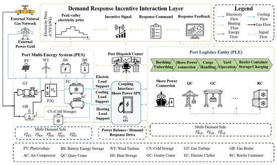
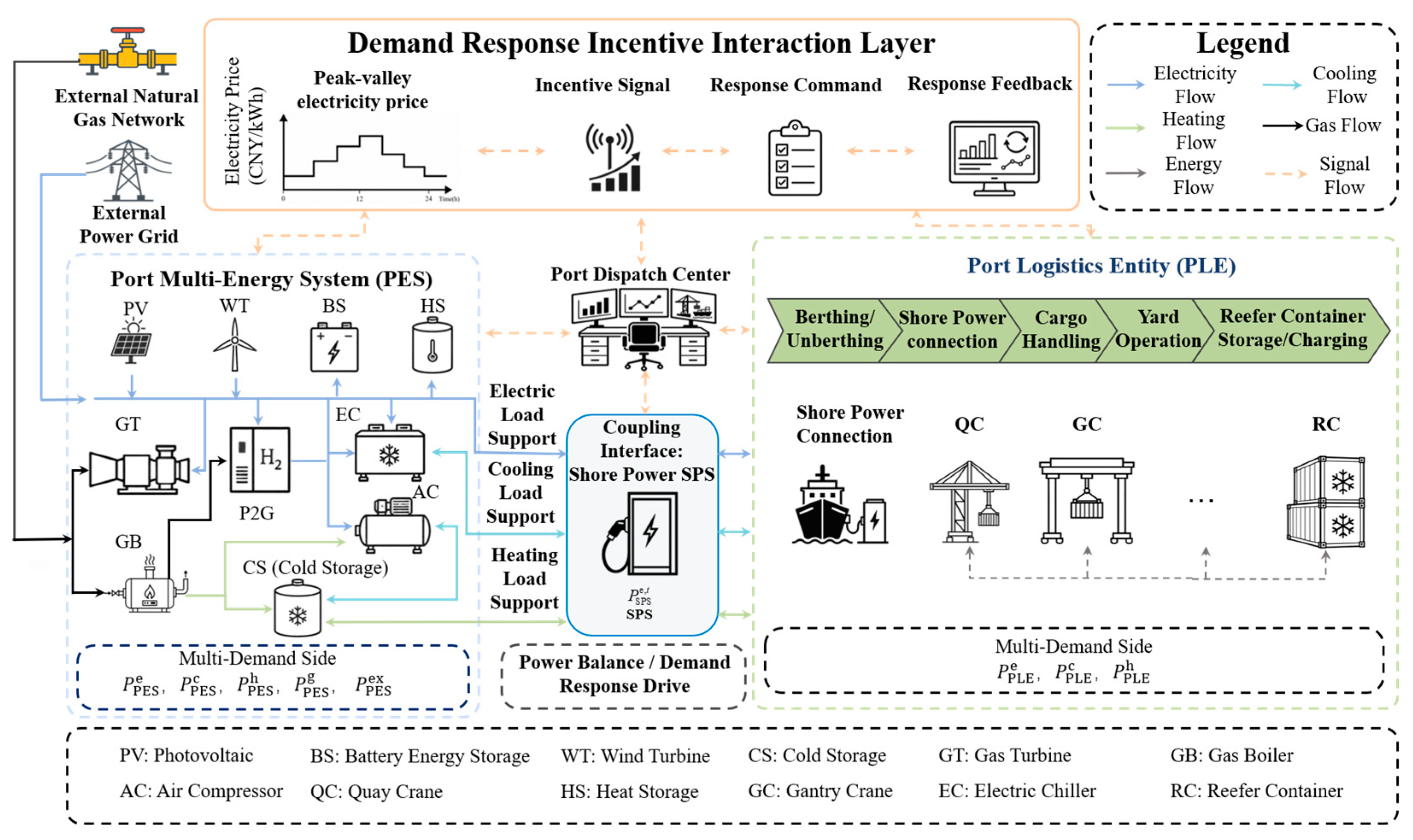
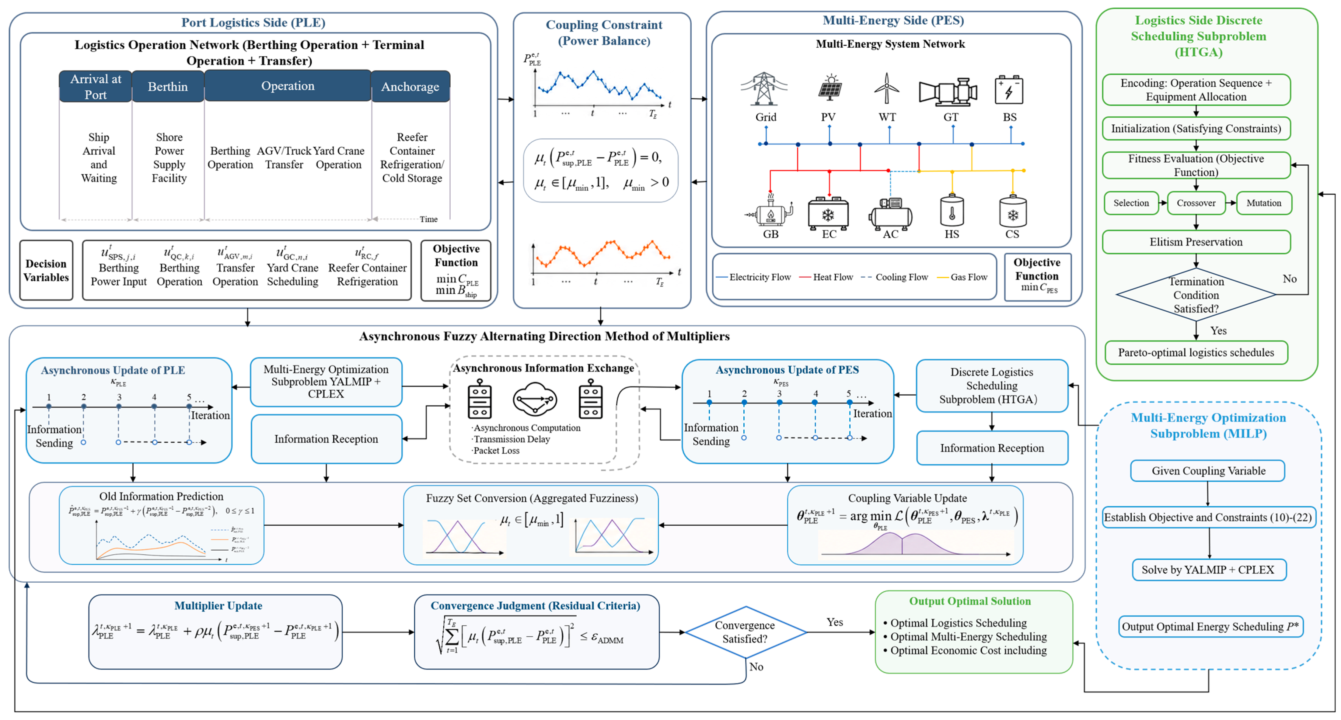
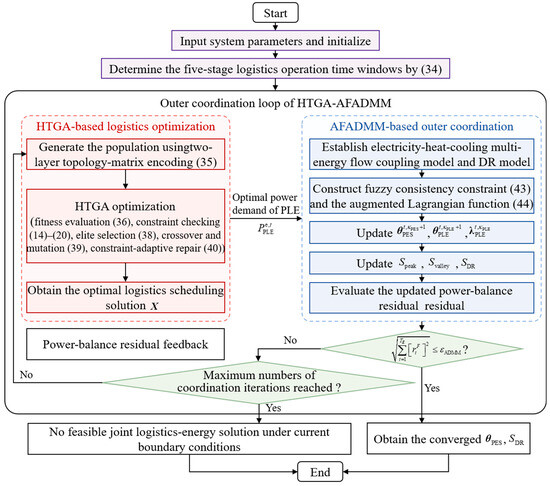
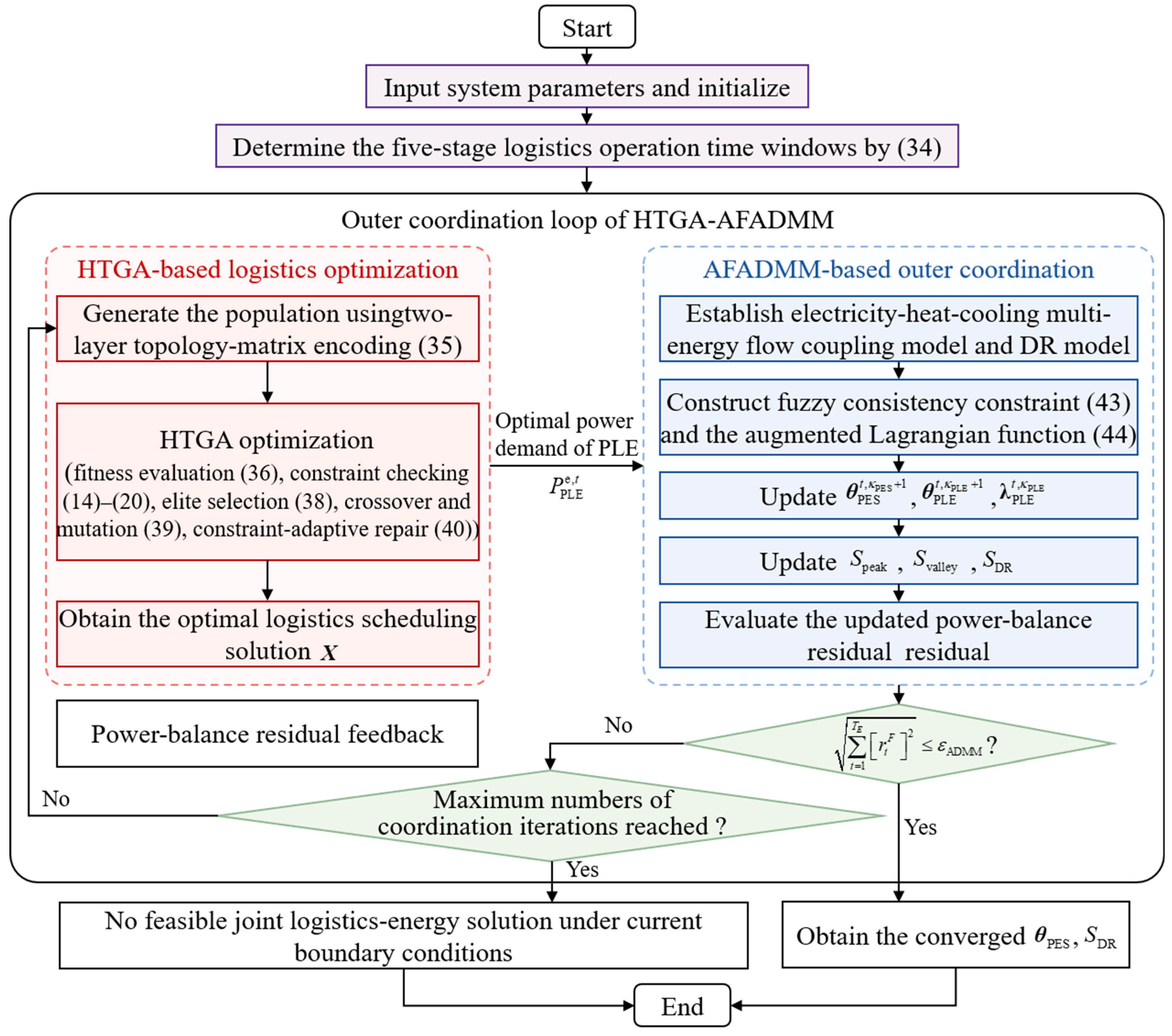
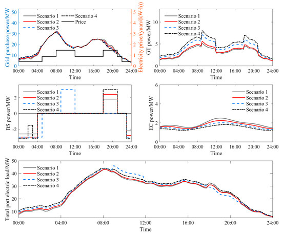
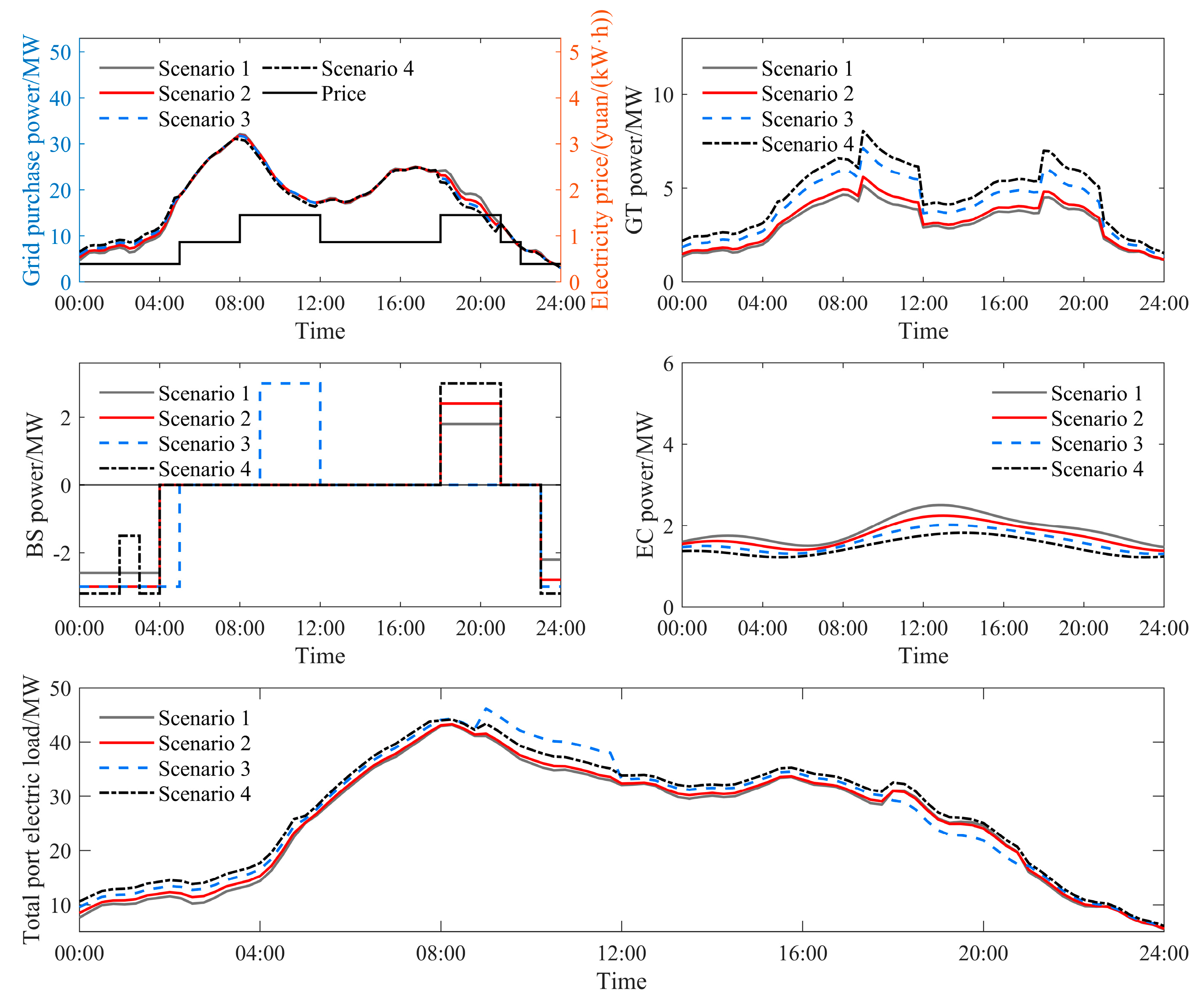
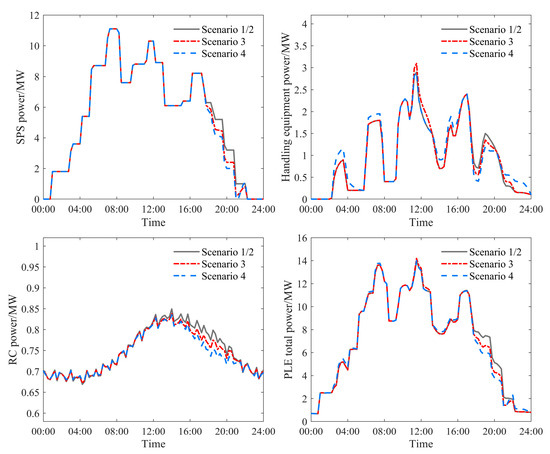
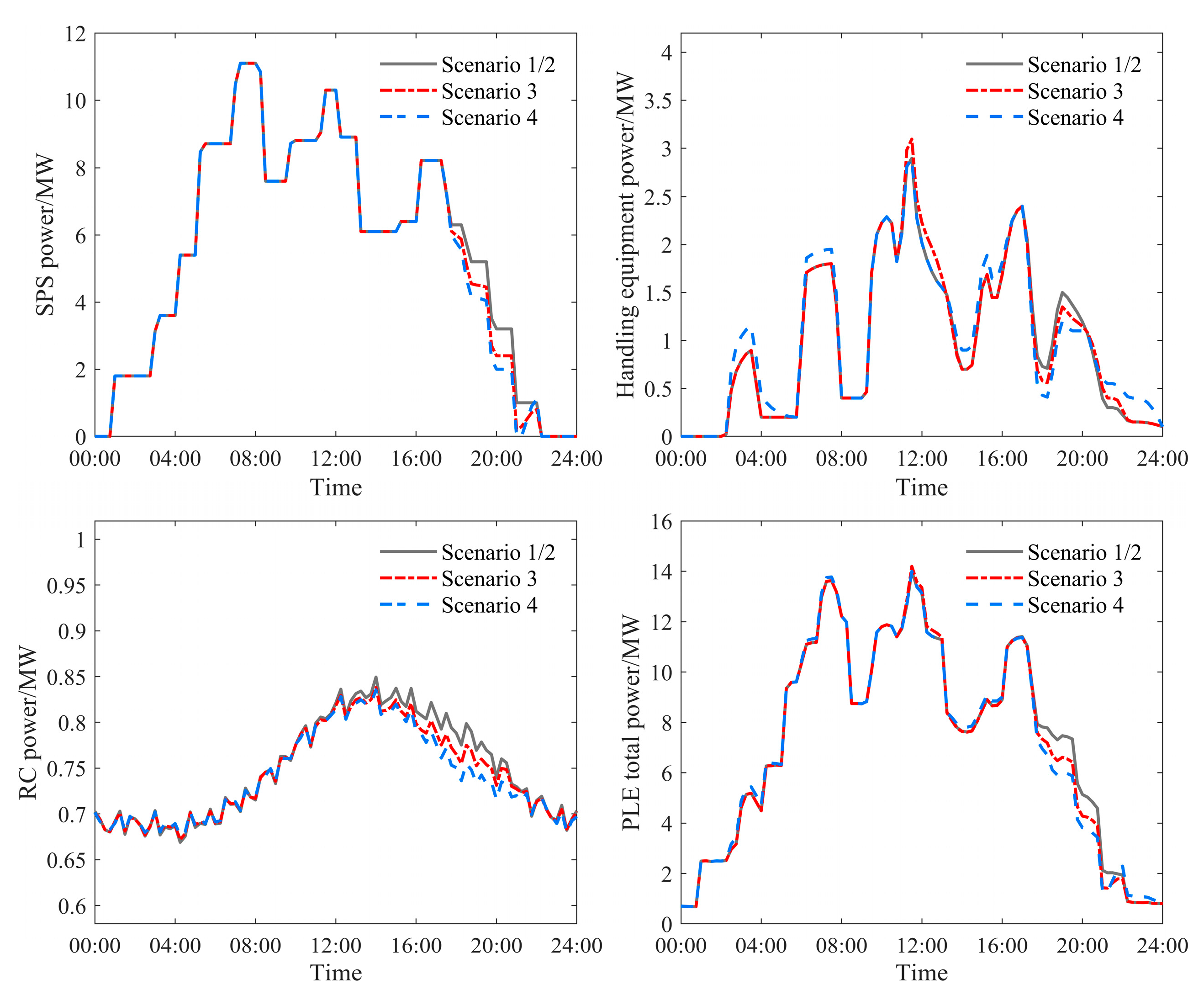
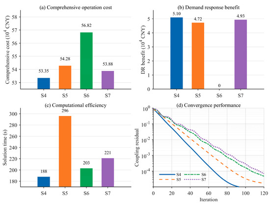
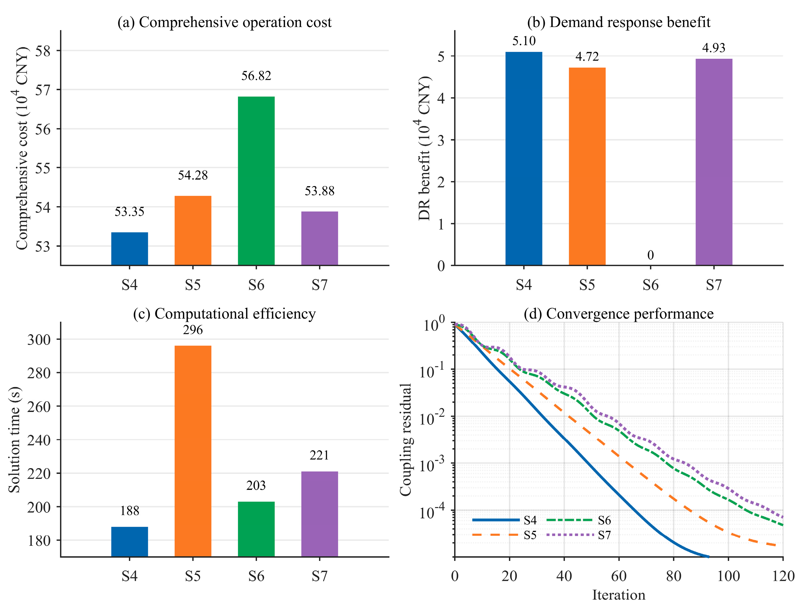
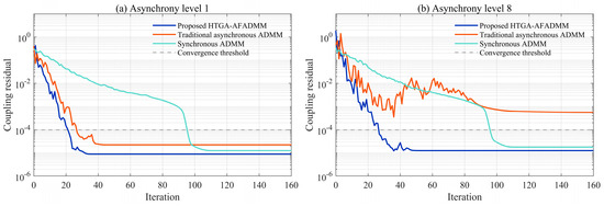
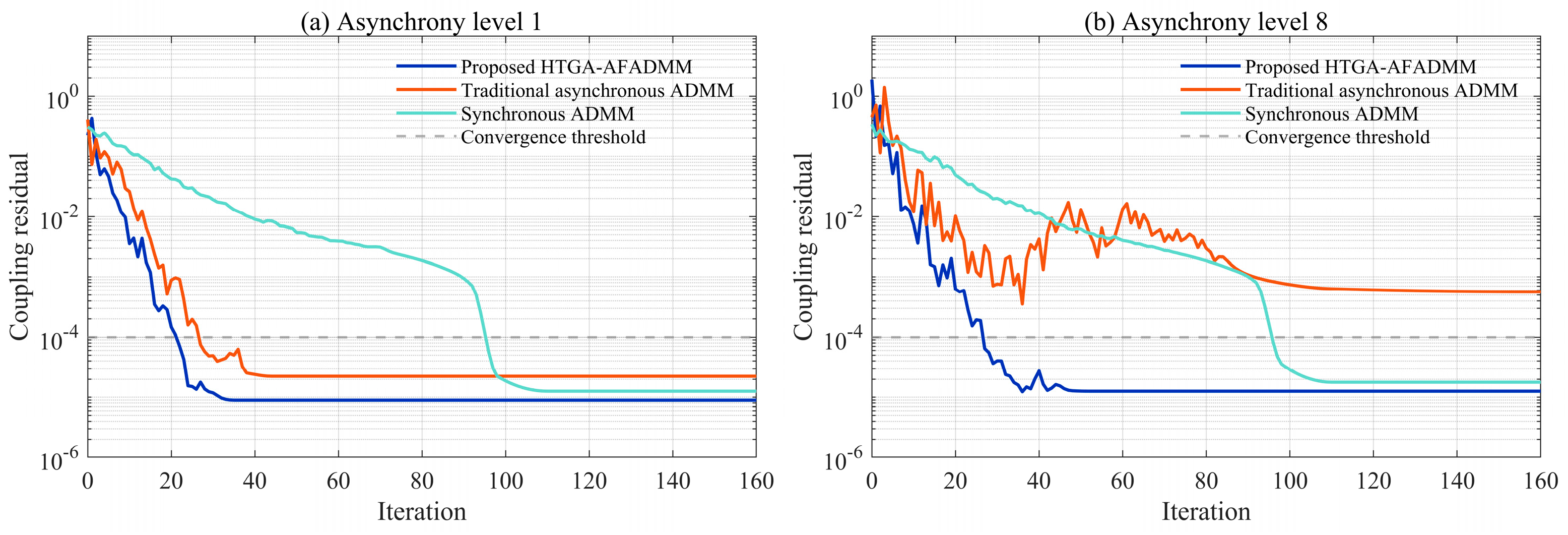
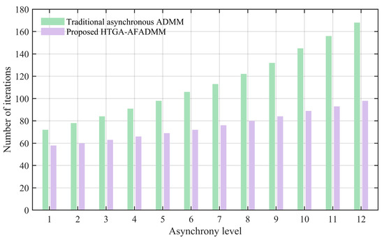
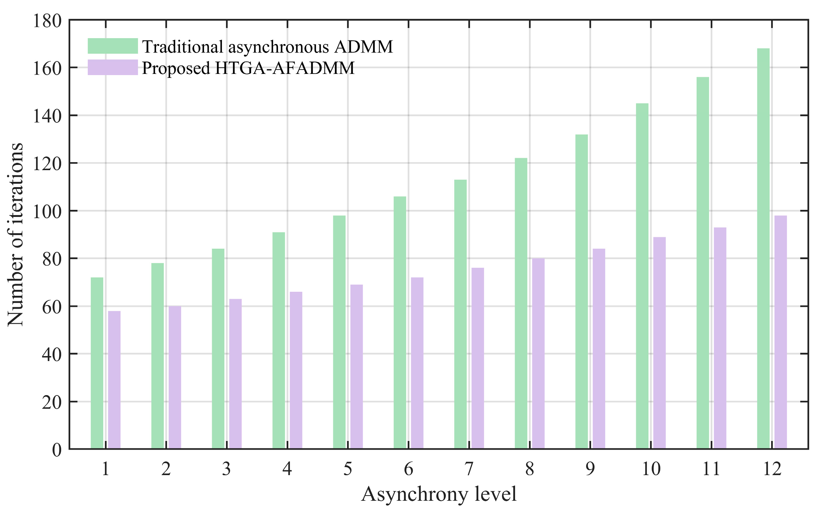
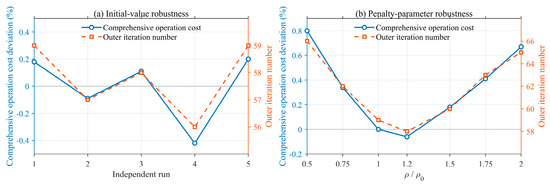
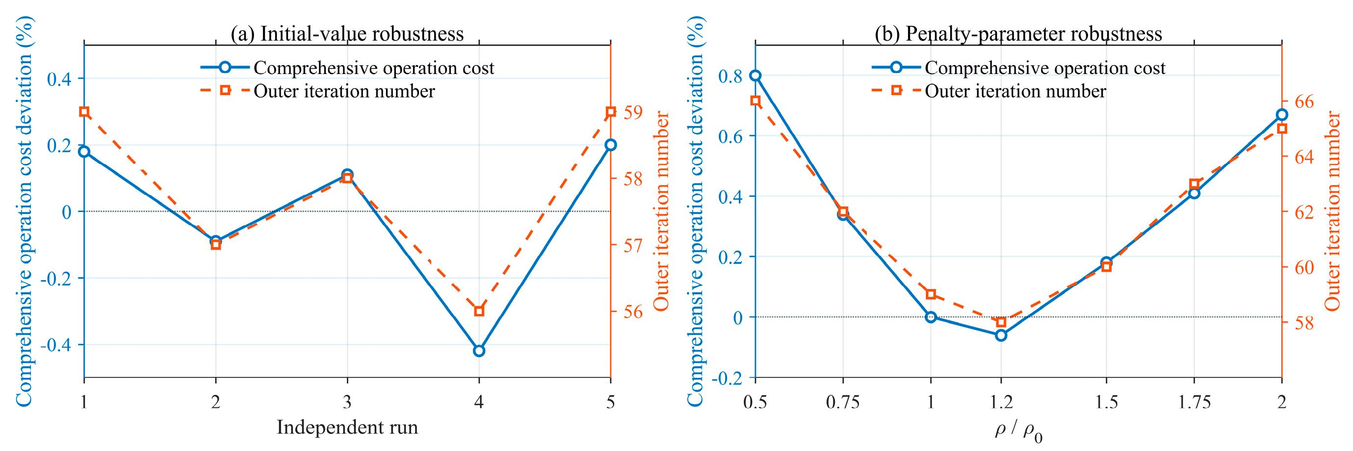
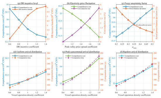
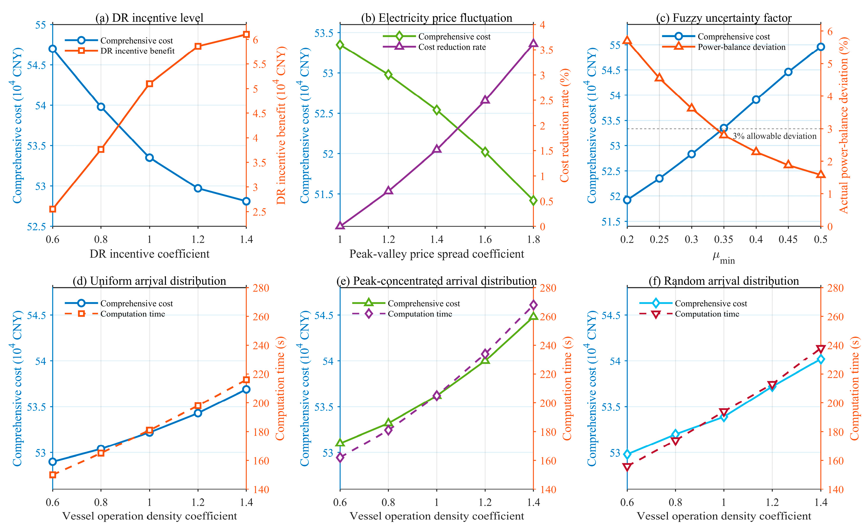

Disclaimer/Publisher’s Note: The statements, opinions and data contained in all publications are solely those of the individual author(s) and contributor(s) and not of MDPI and/or the editor(s). MDPI and/or the editor(s) disclaim responsibility for any injury to people or property resulting from any ideas, methods, instructions or products referred to in the content. |
© 2026 by the authors. Licensee MDPI, Basel, Switzerland. This article is an open access article distributed under the terms and conditions of the Creative Commons Attribution (CC BY) license.