


Abstract
As inverter-based renewable generation increases, load modeling from ambient measurements is important for power-system stability assessment. Under ambient conditions, voltage and frequency variations are small, whereas time-varying nominal power can substantially affect load-power variation. If nominal-power variation is not considered, it may be misattributed to voltage- and frequency-dependent load responses, resulting in biased parameter estimates. Because this misattribution depends on the variations within each time window, single-window estimation may suffer reduced accuracy. This study proposes a method that models time-varying nominal power using an autoregressive moving-average model to separate nominal-power variation from voltage- and frequency-dependent load responses and aggregates validation errors across multiple time windows to reduce dependence on any specific window. Numerical simulations under two nominal-power variation levels were compared with single-window estimation and a previously proposed sensitivity-based window-selection method. When the maximum 100 s peak-to-peak nominal-power variation was 1.0% of the mean nominal power, the proposed method achieved an overall error of 0.100, 86% lower than the mean single-window error and 79% lower than the best sensitivity-based result. Additional analyses under modified identification and data-generation conditions showed that the proposed method generally maintained comparatively low identification errors, although accuracy varied with the conditions.
1. Introduction
As the penetration of renewable energy increases, the share of synchronous generation declines, reducing power-system inertia [1]. Accurate stability assessment has therefore become increasingly important [2,3]. Such assessments require appropriate models not only of generators and networks but also of the response characteristics of aggregated loads [4,5,6]. Accurate representation of the voltage- and frequency-dependent characteristics of aggregated loads is essential for reliable stability assessment and the design of effective control and operational strategies. Simplified load models, such as the constant-power model, cannot represent changes in load power caused by voltage and frequency variations. Their use may therefore lead to discrepancies between simulated and actual load responses [7,8,9,10]. Consequently, power-system analyses require load models that appropriately account for both voltage and frequency dependence.
Quantitative characterization of load behavior requires the identification of load-model parameters from measured data or load composition data. Load model identification methods are broadly classified into component-based and measurement-based approaches [4,11]. Component-based approaches construct aggregate load models from the characteristics and proportions of individual load devices, providing a clear physical interpretation [12,13,14]. Their practical application is limited by the difficulty of obtaining and continuously updating detailed load-composition data because load composition is diverse and changes over time [5,15]. In contrast, measurement-based approaches directly identify aggregate load characteristics from measurement data collected at locations such as substation buses [16,17]. Conventional measurement-based approaches often rely on responses to large disturbances to obtain sufficiently informative variations for load model identification; however, such disturbances do not occur frequently in actual power systems, which can limit their application to continuous load model identification [18]. Recent advances in the deployment of phasor measurement units (PMUs) have changed this situation. PMUs enable the continuous acquisition of synchronized, high-resolution time-series data on power, voltage, and frequency. These data enable load model identification from ambient measurements without requiring large disturbances [15,18,19,20,21].
Despite these advances, load model identification from ambient measurements remains challenging. First, voltage and frequency variations are much smaller than those observed during faults or large disturbances. In this situation, the voltage- and frequency-dependent variation in load power is also small, leading to weak parameter identifiability. Measurement noise, data-processing procedures, and load-model assumptions can therefore have a relatively large influence on the identification results [22,23,24]. A second challenge is the treatment of temporal changes in aggregate load conditions reflected in ambient measurements. In actual power systems, the aggregate load varies over time because of changes in customer behavior, device switching, and load composition. Previous studies have addressed these temporal changes by recursively updating load-model parameters using methods such as recursive least squares (RLS). These methods aim to track time-varying load characteristics [25,26,27].
Temporal variations in measured load power arise not only from changes in load characteristics but also from variations in nominal power. Nominal power represents the underlying demand level. In ambient measurements, voltage and frequency vary only slightly, so the associated voltage- and frequency-dependent load responses are small. Consequently, nominal-power variation has a relatively greater influence on parameter identification under ambient conditions than under disturbance conditions, where larger voltage and frequency excursions produce more pronounced load responses. One approach to mitigating this issue is to select time windows less affected by nominal-power variation. Rizvi et al. [28] proposed a sensitivity-based window-selection method. They noted that identification accuracy decreases in time windows containing abrupt variations in nominal power or changes in load characteristics. Their method selects suitable time windows based on the apparent sensitivity of load power to voltage. This method thereby reduces the influence of nominal-power variation and changes in load characteristics by excluding unsuitable windows.
However, selecting appropriate time windows alone does not resolve the fundamental ambiguity between nominal-power variation and voltage- and frequency-dependent load responses. When nominal power is assumed constant within a window, its variation may be misattributed to voltage- and frequency-dependent load responses, biasing the identified parameters. Moreover, even among windows considered suitable for identification, the estimates may vary with the voltage, frequency, and nominal-power variations contained in each window. In practical power systems, the true load-model parameters are unknown, making it difficult to determine in advance which window is most informative. The load model must therefore represent time-varying nominal power and voltage- and frequency-dependent load responses as distinct components. To reduce dependence on the characteristics of any single time window, the identification framework must determine the final parameters using information from multiple time windows.
This study proposes a robust load-model parameter identification method for ambient measurements that accounts for nominal-power variation. We consider an aggregate load at the distribution-substation level. The proposed method represents measured load power using a load model that explicitly distinguishes time-varying nominal power from voltage- and frequency-dependent load responses. To facilitate this separation, we model nominal power as a temporally correlated process using a time-series model. To reduce dependence on any specific time window, the method identifies load-model parameters by evaluating results from multiple time windows.
The numerical validation focuses on controlled conditions with prescribed true load-model parameters and nominal-power trajectories, allowing the identification performance to be evaluated directly against known true values.
The main contributions of this study are as follows:
- We propose an identification method that explicitly represents time-varying nominal power and imposes temporal constraints using a time-series model. This formulation facilitates the distinction between nominal-power variation and voltage- and frequency-dependent load responses in measured load power.
- We develop a robust identification framework that reduces dependence on any specific time window by determining the load-model parameters from validation errors aggregated across multiple time windows.
- We evaluate the proposed method through numerical simulations under different levels of nominal-power variation and additional identification and data-generation conditions. We compare it with single-window estimation and sensitivity-based window selection to assess its parameter identification accuracy across the examined conditions.
The remainder of this paper is organized as follows. Section 2 formulates the load-model parameter identification problem for ambient measurements while accounting for nominal-power variation. It also explains the need to separate nominal-power variation from voltage- and frequency-dependent load responses and to reduce dependence on any specific time window. Section 3 presents the proposed method, which models the temporal variation in nominal power and identifies load-model parameters with reduced dependence on any specific time window. Section 4 describes the simulation model, nominal-power variation conditions, comparison methods, parameter settings, and evaluation metrics used in the numerical experiments. Section 5 examines the effect of nominal-power variation on parameter identification and evaluates the identification performance of the proposed method across the examined conditions through comparisons with single-window estimation and sensitivity-based window selection. Finally, Section 6 presents the conclusions and directions for future work.
2. Load-Model Parameter Identification Under Nominal-Power Variation
This section formulates the load-model parameter identification problem from ambient measurements under time-varying nominal power. We first define the measurement setting and introduce a load model that represents time-varying nominal power and voltage- and frequency-dependent load responses as distinct components. We then describe the identification challenges associated with unobservable nominal power and single-window estimation.
2.1. Load Model Representation with Nominal-Power Variation
We consider an aggregate load downstream of a measurement point, where synchronized time-series measurements of active power, voltage, and frequency are available. We treat the aggregate load as an unknown system component and identify its load-model parameters from these measurements. To represent time-varying nominal power and voltage- and frequency-dependent load responses as distinct components, we model measured load power as their product. Under nominal-power variation, the identification problem therefore requires both identification of the load-model parameters and estimation of the time-varying nominal power.
The load-model parameters govern how variations in the measured system quantities affect load power. The multiplicative formulation described above is consistent with commonly used static load models, in which load power is represented by a reference power scaled by a voltage- and frequency-dependent response [29]. In this study, the conventional reference power is treated as a time-varying quantity to represent temporal changes in the underlying demand level. The estimated load power at time , , is expressed as
where denotes the time-varying nominal power , the measured system quantities, and the load-response function parameterized by . During the analysis period, the overall demand level of the aggregate load varies over time in response to the collective activities of customers [30,31], and these temporal changes are represented by . In contrast, we assume that the relative composition of the devices constituting the aggregate load and their dominant voltage- and frequency-dependent response characteristics do not change substantially over the same period. Accordingly, the load-model parameters are treated as constant during the analysis period.
2.2. Challenges in Load-Model Parameter Identification Under Time-Varying Nominal Power
As shown in Equation (1), load power is represented as the product of nominal power and the load-response function. However, only the combined load power is observed at the measurement point. Nominal power itself cannot be directly observed. When identifying the load-model parameters from measured load power, the contribution of nominal-power variation must therefore be distinguished from voltage- and frequency-dependent load responses. If nominal power is treated as an independent unknown at each time step, infinitely many combinations of nominal power and load-model parameters can explain the measured load power. This makes it difficult to distinguish nominal-power variation from voltage- and frequency-dependent load responses. Load-model parameter identification from ambient measurements therefore requires a framework that constrains the temporal evolution of unobservable nominal power and distinguishes it from voltage- and frequency-dependent load responses.
In addition, identification based on a single time window may depend on the voltage, frequency, and nominal-power variations contained in that window. This dependence becomes more pronounced when nominal-power variation is large or exhibits a temporal pattern that is difficult to distinguish from the voltage- and frequency-dependent load responses. Because the true load-model parameters are unknown in practical power systems, the most informative time window cannot be determined in advance. A robust identification framework must therefore reduce dependence on any specific time window.
3. Load Model Identification Method
This section presents a method for identifying load-model parameters from ambient time-series measurements while accounting for time-varying nominal power. The proposed method separates nominal-power variation from voltage- and frequency-dependent load responses contained in measured load power. It also evaluates candidate parameters across multiple time windows to reduce dependence on the characteristics of any specific window. The following subsections define the time windows, describe the time-series representation of nominal power, explain the estimation of nominal power and load power, and present the parameter identification procedure based on multiple time windows.
3.1. Overview of the Proposed Identification Method
The proposed method takes synchronized time-series measurements of voltage, frequency, and load power under ambient operating conditions as inputs and identifies a single set of load-model parameters for the entire analyzed time series. It also explicitly treats nominal power as a time-varying quantity and estimates its temporal variation separately from the load-response component. Single-window estimates may depend on the characteristics of the analyzed window. To reduce this dependence, the proposed method aggregates validation errors across multiple time windows and selects the load-model parameters that provide consistent performance over the entire analyzed time series.
Figure 1 illustrates the workflow of the proposed method. First, we collect synchronized time-series measurements of voltage, frequency, and load power at the target measurement point. We then divide the measured time series into multiple time windows. Each window is further divided into a training period and a validation period. The training period is used to estimate a time-series model representing the temporal evolution of nominal power, whereas the validation period is used to evaluate each candidate parameter combination. For each time window, we consider combinations of load-model parameters and candidate orders of the time-series model. For each candidate combination, we estimate a time-series model that captures the temporal dependence of nominal power using the training data. We then use the estimated model to predict nominal power and load power over the validation period. The difference between the measured and estimated load power is calculated as the validation error.
Figure 1.
Workflow of the proposed method. The green and blue dashed boxes indicate the loops over time windows and candidate parameter sets, respectively.
We repeat this procedure for all candidate combinations and time windows. This produces a validation error for each candidate combination in each window. An evaluation based on a single window may be strongly affected by the voltage, frequency, and nominal-power variations specific to that window. We therefore aggregate the validation errors across multiple windows and select the load-model parameters that are appropriate for the entire analyzed time series.
Through this procedure, the proposed method accounts for time-varying nominal power while reducing the dependence of the identified load-model parameters on any specific time window.
3.2. Definition of Time Windows
In this study, we divide the ambient time-series data into multiple time windows. Estimation is performed separately within each window, and the results obtained across all windows are used to identify a common set of load-model parameters for the entire time series.
Let and denote the window length and window shift, respectively, in seconds. The -th time window begins seconds after the start of the analyzed time series and contains seconds of data. Here, denotes the window index, where , and is the total number of time windows.
When the window shift is shorter than the window length, adjacent time windows overlap. Consequently, the validation errors obtained from different windows may be statistically dependent because some observations can appear in different roles across neighboring windows. In the proposed framework, these window-wise validation errors are used as model-selection criteria at multiple temporal positions and are not treated as statistically independent test results.
3.3. Representation of Time-Varying Nominal Power
For an aggregate load at the distribution-substation level, nominal power under ambient operating conditions is not expected to vary substantially and independently at each time step. Instead, it evolves with temporal dependence between adjacent time steps. We therefore represent nominal power as a time series related to its past values rather than treating it as an independent unknown at each time step.
To represent this temporal evolution, we use an autoregressive moving-average (ARMA) model. Within each time window, nominal power is expressed in terms of its past values and error terms as follows:
where is the constant term, is the -th autoregressive coefficient, is the -th moving-average coefficient, and is the error term at time . The parameters and denote the autoregressive and moving-average orders, respectively. The autoregressive terms account for the relationship between the current and past values of nominal power. The moving-average terms account for the effects of past error terms. This representation allows the temporal evolution of nominal power to be approximated as a time series with temporal dependence.
3.4. Estimation of Nominal Power and Load Power
Within each time window, the time-series data are divided chronologically into an earlier training period and a subsequent validation period . This partition preserves the temporal order of the measurements. We consider candidate combinations , where denotes the load-model parameters, and and denote the AR and MA orders, respectively.
For each candidate combination, the ARMA coefficients and other internal variables are estimated using the training period. The fitted ARMA model is then applied to the subsequent validation period to estimate nominal power and load power and to calculate the corresponding validation error. Thus, within each individual time window, the validation data are not used to fit the ARMA model for that same window. The validation error is used to compare the candidate combinations and select the load-model parameters and ARMA orders. Therefore, the validation period serves as model-selection data and is not treated as an independent test interval.
For each candidate combination, we perform the following procedure.
First, we estimate the ARMA model parameters for nominal power using the training data. Based on Equation (1), the estimated load power is calculated from the estimated nominal power and the load-response function as
where and denote the estimated nominal power and load power, respectively.
For each candidate combination , we hold , , and fixed and estimate the ARMA coefficients, constant term, and initial nominal power by minimizing the training loss between the measured and estimated load power over the training period. The training loss is defined as
where denotes the loss function between the measured and estimated load power. The optimization variables include the initial nominal power, constant term and the ARMA model parameters:
Next, we use the ARMA model parameters estimated during the training period to estimate nominal power over the validation period . We then calculate the estimated load power using Equation (3). The validity of each candidate combination is evaluated based on the error between the measured and estimated load power. The validation error is defined as
Within each time window, this procedure estimates nominal power and load power, and calculates the load-power validation error for each candidate combination of load-model parameters and ARMA model orders.
3.5. Robust Load-Model Parameter Identification Based on Multiple Time Windows
Let denote the validation error for candidate combination in the -th time window. For each candidate combination, we aggregate the validation errors obtained from the time windows. The integrated evaluation metric is defined as
where denotes an aggregation operator that summarizes the validation errors obtained from the multiple time windows into a representative value.
We then select the candidate combination that minimizes the integrated evaluation metric:
Among the selected parameters, is taken as the final set of load-model parameters for the entire analyzed time series.
Thus, Equations (6) and (7) constitute the model-selection stage of the proposed framework. Each candidate combination is evaluated by aggregating its validation errors across multiple time windows, and the combination that minimizes the integrated validation metric is selected. When adjacent time windows overlap, the validation errors obtained from different windows are not assumed to be statistically independent. The integrated validation metric is used solely for candidate selection and is neither interpreted as an estimate of independent test performance nor regarded as the final measure of parameter-identification accuracy.
4. Numerical Experiment Setup
This section describes the numerical experiments conducted to evaluate the proposed method. Because the true load-model parameters and nominal-power trajectories are generally unavailable in field measurements, we generate time-series data through dynamic simulations with prescribed values to quantitatively evaluate identification accuracy. We then estimate the load-model parameters from the generated data and compare the estimates with their prescribed values.
We first construct a simplified power-system model using PSCAD/EMTDC [32]. We prescribe the temporal variation in nominal power and the load-model parameters. These prescribed values serve as the true values in the numerical experiments. We then perform dynamic simulations and record time-series data for voltage, frequency, and active power at the measurement point. The proposed and comparison methods are subsequently applied to the generated data. To isolate the effects of time-varying nominal power and the examined identification conditions on parameter estimation, the present numerical simulations use ideal measurement signals generated directly from PSCAD, without additional measurement noise or PMU-specific frequency-estimation errors.
The numerical experiments consist of a primary evaluation and additional analyses under modified conditions. The primary evaluation is conducted to clarify the identification characteristics of the proposed method and compare its performance with the comparison methods under representative conditions. The additional analyses are conducted to examine the extent to which the identification results depend on specific experimental and identification settings and to evaluate whether the proposed method maintains its identification performance under the examined changes in these conditions. The specific conditions considered in these analyses are described together with the corresponding settings below.
4.1. Simulation Model and Data
4.1.1. Power System Model
The numerical experiments use the simplified power-system model shown in Figure 2. The model was implemented in PSCAD 5.0.2 and consists of two thermal synchronous generators, a transmission network, transformers, and loads. Both generators are equipped with LAT1 automatic voltage regulators and LPT1 governor/turbine models, and their inertia constants are 4.0 s. The generators are interconnected through a 500-kV transmission network, and the target load is connected on the 275-kV side downstream of the measurement point. Detailed network and component parameters are provided in Appendix A. System operators generally have access to information on the generators and network. In contrast, they cannot directly observe the composition and operating conditions of customer-side loads. We therefore treat the aggregate load connected downstream of the measurement point as the target load for parameter identification.
Figure 2.
Power-System Model.
We record active power, voltage, and frequency at the measurement point. In addition to the target load, the model includes other loads whose aggregate active power is denoted by . represents the effect of loads other than the target load on the system operating conditions and is treated as an unobserved quantity in the parameter-identification procedure. Accordingly, only the active power, voltage, and frequency measured at the measurement point are used for identification, and is not used as an input to the proposed method. This study focuses on the active-power characteristics of the load. Reactive-power characteristics are outside the scope of this study.
4.1.2. Load Model
To instantiate the general load-model formulation introduced in Section 2.1, we adopt a voltage- and frequency-dependent exponential load model. The exponential model is one of the most frequently used static load models and directly represents the active-power responses to voltage and frequency through the two exponents and [29]. Its low-dimensional parameterization facilitates interpretation of the effects of time-varying nominal power and time-window characteristics on parameter identification and keeps the candidate-parameter search tractable. We therefore use it as a representative static load model for evaluating the central identification problem considered in this study. The estimated active power at time is expressed using nominal power, measured voltage, measured frequency, and the load-model parameters as
where denotes the nominal power at time , and and denote the measured voltage and frequency, respectively. and are the nominal voltage and nominal frequency, respectively. The parameters and characterize the active-power responses to voltage and frequency variations, respectively.
The proposed identification framework is not mathematically restricted to the exponential model. For another static load model that can be expressed in the multiplicative form of Equation (1), such as a ZIP-type model, the framework can in principle be applied by replacing the load-response function and redefining the candidate parameter set and its constraints.
In the present numerical experiments, the exponential load model is used for both data generation and parameter identification so that the identification accuracy can be directly evaluated against prescribed true values of and .
4.1.3. Data-Generation Conditions
Table 1 summarizes the simulation conditions used to generate the time-series data for the primary evaluation.
Table 1.
Simulation conditions for time-series data generation in the primary evaluation.
The prescribed true load-model parameters shown in Table 1 are used in the primary evaluation. To examine the identification performance for a different parameter combination, an additional simulation is conducted with . For the voltage exponent, was selected as a value lower than the primary value of , with reference to the worldwide average active-power voltage exponent of approximately reported for aggregated loads in [29]. The frequency exponent is selected independently as an additional test value to examine the effect of changing the prescribed true parameters, rather than to represent a specific value reported in the literature.
4.2. Nominal-Power Variation Conditions
To evaluate the effect of nominal-power variation on load-model parameter identification, we generate time-series data using prescribed nominal-power trajectories. We define nominal-power variation conditions by scaling the amplitude of a temporal profile obtained from actual urban demand data [33].
The mean nominal power of the target load over the analysis period is denoted by . The variable denotes the temporal profile obtained from the urban demand data, and denotes the prescribed nominal-power variation rate. We scale such that the largest peak-to-peak variation in nominal power over any 100 s interval equals . To determine the scaling factor, we first locate the 100 s interval in which has the largest difference between its maximum and minimum values. We denote this difference by . The scaling factor is then defined as
Using this scaling factor, we define nominal power as
where denotes the mean of over the analysis period. This formulation maintains the mean nominal power at . It also preserves the temporal pattern of the urban demand data while adjusting only its variation amplitude.
Figure 3 shows the two temporal profiles considered in this study. Profile 1 is the 1100 s profile used in the primary evaluation. For the additional analysis examining the influence of the nominal-power trajectory, Profile 2 is taken from the 1100 s segment immediately following Profile 1 in the same urban demand dataset to avoid arbitrary selection of the additional profile. Thus, the two profiles correspond to consecutive segments of the original demand data. Both profiles are scaled using the same procedure described above.
Figure 3.
Temporal profiles obtained from the urban demand data and used to generate the nominal-power trajectories: (a) Profile 1; (b) Profile 2. Profile 2 corresponds to the 1100 s segment immediately following Profile 1 in the original dataset.
Based on short-term variations observed in actual urban demand data, we consider two nominal-power variation rates: and . An analysis of 100 s intervals showed variation rates of approximately or higher, with a mode of approximately . We therefore use these two values as representative nominal-power variation conditions.
The condition represents relatively small nominal-power variation, under which nominal-power variation and voltage- and frequency-dependent load responses are comparatively easy to separate. In contrast, represents a more challenging condition in which nominal-power variation has a greater influence on parameter identification. We assign the same true load-model parameters under both conditions and evaluate the identification accuracy and stability of each method over a realistic range of nominal-power variation.
4.3. Comparison Methods
To evaluate the effectiveness of the proposed method in accounting for nominal-power variation, we compare it with single-window estimation and sensitivity-based window selection. These comparisons allow us to evaluate how the treatment of nominal-power variation and the use of time windows affect the identification results.
4.3.1. Single-Window Estimation
Single-window estimation identifies the load-model parameters separately within each time window constructed from the target time-series data. For each window, we calculate the load-power validation error for every candidate combination of load-model parameters and ARMA model orders. We then select the load-model parameters associated with the minimum validation error as the estimate for that window. This method provides a separate parameter estimate for each time window. These estimates allow us to examine how nominal-power variation and the voltage and frequency variations contained in each window affect the identification results.
4.3.2. Sensitivity-Based Window Selection
Sensitivity-based window selection accounts for differences in parameter identifiability among time windows by selecting intervals suitable for parameter estimation. Specifically, the method extracts intervals in which the relationship between load power and the measured system variables remains relatively consistent. It then estimates the load-model parameters using the selected intervals. Following the sensitivity-based window-selection approach of Rizvi et al. [28], which uses the apparent sensitivity of load power to voltage, this study extends the criterion to consider apparent sensitivities to both voltage and frequency. This window-selection process aims to reduce the effects of changes in load composition and nominal-power variation on parameter identification. Appendix B presents the detailed implementation of the sensitivity-based window-selection method.
4.4. Parameter Setting
Table 2 summarizes the search ranges for the load-model parameters used in all methods and the candidate AR and MA orders used in the primary evaluation to represent temporal variations in nominal power.
Table 2.
Parameter search settings for the primary evaluation.
The candidate AR orders shown in Table 2 are used in the primary evaluation. To examine the influence of the AR-order candidate set on the identification results, additional analyses are conducted using and , while the other parameter-search settings are kept unchanged.
Table 3 presents the time-window settings used for the proposed method and single-window estimation.
Table 3.
Time-window settings for the proposed method and single-window estimation.
As shown in Table 3, each 200 s time window was divided chronologically into the first 150 s for training and the subsequent 50 s for validation. With a sampling interval of 1 s, these periods contained 150 and 50 samples, respectively. Considering that the maximum candidate MA order was 40, the validation period was set to 50 s as a practical evaluation interval longer than the maximum candidate order. The remaining 150 s were used as the training period for estimating the ARMA model parameters.
For the primary evaluation, the median is used as the aggregation operator in Equation (6). The median was selected to reduce excessive influence from any particular time window and to represent the typical validation performance across multiple time windows. To examine the influence of the aggregation operator, additional analyses are conducted using the arithmetic mean and the minimax criterion. For the minimax criterion, the maximum validation error across the time windows is used as the aggregation metric, so that the candidate combination minimizing the worst-window validation error is selected.
Table 4 summarizes the settings for the sensitivity-based window-selection method. In the experiments conducted by Rizvi et al. [28], was used as the threshold for the apparent voltage sensitivity. In addition to the apparent voltage sensitivity, this study considers the apparent frequency sensitivity. We therefore introduce as the threshold for a sensitivity criterion that jointly considers both apparent sensitivities. We use as a representative setting close to that adopted in the original study. Under conditions with large nominal-power variation, its influence may appear as changes in the apparent sensitivity, and a strict threshold may prevent the selection of any time window. To account for the influence of nominal-power variation on the apparent sensitivities and to improve the feasibility of window selection, we also consider a relaxed threshold of . When the settings with and still yield no selected time window for some window-length settings, is additionally examined as a more strongly relaxed condition. This additional threshold is used to examine whether further relaxation enables window selection and how such relaxation affects the resulting identification accuracy.
Table 4.
Settings for sensitivity-based window selection.
4.5. Evaluation Metrics
We use two error metrics that have distinct roles in the identification and evaluation procedures: the load-power validation error and the load-model parameter identification error. The load-power validation error is calculated over the validation period and is used to compare the candidate combinations of load-model parameters and ARMA orders. Therefore, the validation error serves as a model-selection criterion and is not treated as an independent test metric. In contrast, the parameter identification error is calculated after the candidate-selection procedure and is used to evaluate how closely the selected load-model parameters match their prescribed true values.
The load-power validation error is calculated from the difference between the measured active power and the active power estimated by the load model over the validation period. For each candidate combination of load-model parameters and ARMA orders, the validation error defined in Section 3.4 is expressed as
After each method has completed its parameter-estimation and candidate-selection procedure, we evaluate the identification accuracy of the estimated load-model parameters using the overall parameter identification error, denoted by . Let and denote the estimated parameter values, and let and denote their prescribed true values, respectively. The overall error is defined as
The prescribed true parameter values are not provided to the identification procedure and are not used to estimate the ARMA coefficients, calculate the validation errors, or select the candidate combinations. They are used only after candidate selection to evaluate the parameter identification accuracy in the numerical experiments. Therefore, is a post-selection evaluation metric distinct from the validation error used for candidate selection.
For the proposed method, is calculated using the load-model parameters selected by minimizing the integrated validation metric across multiple time windows.
5. Results and Discussion
This section evaluates the effect of nominal-power variation on load-model parameter identification and the identification performance of the proposed method under the examined conditions.
First, we compare single-window estimation with the proposed method under the primary evaluation conditions. We examine how nominal-power variation and the characteristics of individual time windows affect the identified parameters. We also compare the load-power and nominal-power estimates in a representative time window to clarify why the two methods yield different identification results. We then compare these methods with sensitivity-based window selection and evaluate how the sensitivity threshold and window-length settings affect window selection and identification accuracy. Finally, additional analyses are conducted by changing the aggregation operator, the candidate AR-order set, the nominal-power profile, and the prescribed true load-model parameters to examine the dependence of the identification results on these experimental and identification conditions.
Through these comparisons and additional analyses, we evaluate the proposed framework, which combines ARMA-based modeling of time-varying nominal power with the aggregation of validation errors across multiple time windows.
5.1. Comparison Between Single-Window Estimation and the Proposed Method
This section compares single-window estimation with the proposed method under the primary evaluation conditions and evaluates how aggregating validation errors across multiple time windows affects load-model parameter identification accuracy. We first compare the overall errors and identified parameter values obtained using the two methods. We then examine the estimated load power and nominal power in a representative time window to explain why the two methods yield different identification results.
Figure 4 shows the overall errors of the load-model parameters obtained using single-window estimation and the proposed method.
Figure 4.
Overall error comparison between single-window estimation and the proposed method.
For single-window estimation, the overall error increases with the nominal-power variation rate. This result indicates that larger nominal-power variation reduces identification accuracy. In contrast, the proposed method yields a lower overall error than single-window estimation under both nominal-power variation conditions. Its overall error also remains low as the nominal-power variation rate increases. The difference in identification accuracy between the two methods is particularly pronounced under the larger nominal-power variation condition.
Figure 5 shows the load-model parameters identified separately in each time window and the final parameter values identified using the proposed method.
Figure 5.
Comparison of estimated load-model parameters between single-window estimation and the proposed method. (a) %, (b) %.
Under the condition, the single-window results exhibit some dispersion, but most of the identified values lie near the true values. Under the condition, the distribution becomes wider, and some identified values deviate substantially from the true values. As nominal-power variation increases, its contribution to the observed load-power variation becomes relatively large. This makes it more difficult to separate nominal-power variation from the voltage- and frequency-dependent load responses. Consequently, the identified parameters depend on the magnitudes and temporal patterns of nominal power, voltage, and frequency within each time window.
In contrast, the final parameter values identified using the proposed method lie near the true values under both nominal-power variation conditions. This result is particularly notable under the condition. The proposed method identifies parameter values close to the true values even though the single-window results are widely dispersed. Rather than relying on the validation error from a specific window, the proposed method selects parameters that enable the load model to consistently reproduce load power across multiple time windows.
We next examine the estimated load power and nominal power to clarify why the two methods yield different identification results. Among the 10 single-window results obtained under the nominal-power variation condition, we selected the time window whose overall error was closest to the median as the representative window. In this window, single-window estimation selected the candidate combination The proposed method selected the final candidate combination by aggregating the validation errors across the 10 time windows.
Figure 6 compares the load-power and nominal-power estimates over the validation period of a representative window under the nominal-power variation condition.
Figure 6.
Comparison of load-power and nominal-power estimates in a representative time window under the 1.0% nominal-power variation condition: (a) Load power; (b) Nominal power.
Figure 6a shows that the load-power estimate obtained using single-window estimation closely reproduces the measured load power. This result is expected because single-window estimation selects the candidate combination that minimizes the load-power validation error in the corresponding window. The proposed method shows a slightly larger deviation from the measured load power but still captures its temporal variation. Because the proposed method selects the final candidate combination based on the validation errors across all 10 windows, it does not necessarily minimize the load-power error in the displayed window.
Figure 6b, however, shows that the nominal-power estimate obtained using single-window estimation deviates substantially from the true value throughout the validation period. Load power is expressed as the product of nominal power and the voltage- and frequency-dependent load response. Therefore, an error in the estimated nominal power can be offset by biased load-model parameters. This compensation allowed single-window estimation to reproduce the measured load power even with , which deviates from the true values. Thus, the candidate combination whose load-power estimate best reproduces the measured load power in a single window does not necessarily provide an appropriate separation between nominal power and the load response.
In contrast, the nominal-power estimate obtained using the proposed method accurately captures both the magnitude and temporal variation in the true nominal power. The proposed method also identifies , which is close to the true values of . The proposed method selects a candidate combination that consistently reproduces load power across multiple time windows. These observations indicate that accurate reproduction of load power in a single window is not sufficient for reliable parameter identification.
These results show that single-window estimation may reproduce the load power in a specific window even when nominal power and the voltage- and frequency-dependent load responses are not appropriately separated. This can cause the identified load-model parameters to deviate from their true values. Both single-window estimation and the proposed method use an ARMA model to impose temporal structure on the unobservable nominal power. This representation imposes temporal dependence on the estimated nominal-power trajectory rather than treating nominal power as an independent unknown at each time step. This temporal constraint facilitates the distinction between nominal-power variation and voltage- and frequency-dependent load responses. However, within a single time window, errors in the nominal-power estimate can still be compensated for by biased load-model parameters. The proposed method mitigates this remaining ambiguity by aggregating validation errors across multiple time windows. Consequently, the combined framework of ARMA-based nominal-power modeling and multi-window aggregation identified load-model parameters close to their true values under both nominal-power variation conditions. In the representative window, it also captured the magnitude and temporal variation in nominal power more accurately than single-window estimation.
5.2. Comparison with Sensitivity-Based Window Selection
This section evaluates the identification performance of sensitivity-based window selection through comparisons with single-window estimation and the proposed method under the primary evaluation conditions. Specifically, we examine how the sensitivity threshold and window-length settings affect both the selected time windows and the overall error of the identified load-model parameters. We also evaluate how the nominal-power variation rate affects the number of settings that yield at least one selected window and discuss the differences from the proposed method.
Figure 7 compares the overall errors obtained using single-window estimation, the proposed method, and sensitivity-based window selection. For the sensitivity-based method, the figure shows the minimum, maximum, and median overall errors across the settings that yielded at least one selected window. For , eight settings corresponding to and were examined. Because these thresholds allowed time windows to be selected for all tested window-length settings, further relaxation to was not examined. For , was additionally examined because some settings with and yielded no selected time window. Settings that yielded no selected window were excluded because the load-model parameters could not be identified under those settings.
Figure 7.
Overall error comparison under different nominal-power variation rates. (a) %, (b) %. The gray and orange dashed lines indicate the overall errors of single-window estimation and the proposed method, respectively.
Figure 7 shows a similar trend under both the and conditions. The minimum overall error of the sensitivity-based method is lower than that of single-window estimation. This result indicates that selecting suitable time windows can improve identification accuracy under appropriate settings. However, the median error is comparable to that of single-window estimation, whereas the maximum error is higher. Thus, although the sensitivity-based method can outperform single-window estimation under some settings, its identification accuracy varies with the sensitivity threshold and window-length settings. These settings determine which time windows are selected, and the resulting accuracy therefore depends on the data characteristics of the selected windows.
Under the primary evaluation conditions, the proposed method yields a lower overall error than the minimum error of the sensitivity-based method for both nominal-power variation rates. Specifically, the proposed method yields overall errors of and for and , respectively, whereas the minimum errors of the sensitivity-based method are and . Thus, under these conditions, the proposed method provides higher identification accuracy than any of the sensitivity-based settings examined. At the same time, the minimum errors obtained by the sensitivity-based method show that appropriate window selection can substantially improve identification accuracy compared with single-window estimation. At , the overall error of the proposed method was approximately % lower than the mean overall error of single-window estimation and % lower than the minimum overall error of sensitivity-based window selection .
Table 5 summarizes the number of window-length settings examined for each sensitivity threshold and the number of settings that yielded at least one selected window.
Table 5.
Summary of window-selection results for the sensitivity-based method.
Table 5 shows how the nominal-power variation rate and sensitivity threshold affect the feasibility of window selection. For , all four window-length settings examined with and all four settings with yielded at least one selected window. Therefore, all eight settings examined under this condition allowed parameter identification, and further relaxation to was not required. In contrast, for , none of the four settings with yielded a selected window, whereas two of the four settings with yielded at least one selected window. When the threshold was further relaxed to , all four window-length settings yielded at least one selected window.
The need for a more relaxed threshold under also suggests that the apparent sensitivities vary more substantially as the time window is extended. In the sensitivity-based method, the window is extended in 10 s increments only when the changes in the apparent voltage and frequency sensitivities remain within the specified threshold. Therefore, the difficulty in selecting windows with indicates that intervals satisfying a strict similarity condition are difficult to identify under larger nominal-power variation. Increasing enables more windows to be selected by allowing larger changes in the apparent sensitivities, but the selected windows consequently satisfy a less restrictive similarity criterion. This helps explain why the identification results can depend strongly on the sensitivity threshold and window-length settings.
These results show that sensitivity-based window selection can achieve high identification accuracy when suitable time windows are selected. However, the feasibility of window selection and the resulting identification accuracy depend on the nominal-power variation rate, sensitivity threshold, and window-length settings. In particular, when the apparent sensitivities vary substantially during window extension, an appropriate threshold must balance the strictness of the similarity criterion with the availability of selectable windows. In contrast, the proposed method aggregates validation errors across multiple time windows and does not require an explicit sensitivity-based criterion for selecting individual windows.
5.3. Additional Validation Under Modified Identification and Data-Generation Conditions
To further examine the dependence of the identification results on specific identification settings and data-generation conditions, four additional analyses were conducted by changing the validation-error aggregation operator, the candidate AR-order set, the nominal-power profile, and the prescribed true load-model parameters. In each analysis, only the condition of interest was changed, while the remaining settings were kept consistent with the primary evaluation conditions unless otherwise stated.
5.3.1. Aggregation Operator
To examine the influence of the validation-error aggregation operator on the identification results, three aggregation operators were compared: the arithmetic mean, median, and minimax criterion. The median was used in the primary evaluation, while the other identification and evaluation settings were kept unchanged. For the minimax criterion, the maximum validation error across the time windows was used as the aggregation metric; thus, the candidate combination that minimized the worst-window validation error was selected. The comparison was conducted for both nominal-power variation rates, r = 0.3% and r = 1.0%. Figure 8 compares the overall parameter identification errors obtained using the three aggregation operators.
Figure 8.
Comparison of the overall parameter identification errors obtained using the median, mean, and minimax criterion as the validation-error aggregation operator.
For , the overall errors were , , and when the median, mean, and minimax criterion were used, respectively. For , the corresponding errors were , , and , respectively. Thus, the median yielded the lowest overall parameter identification error under both nominal-power variation conditions, with a particularly pronounced difference under .
The three aggregation operators emphasize different aspects of the window-wise validation errors. The mean reflects average validation performance but can be affected by relatively large errors in individual time windows. The minimax criterion explicitly emphasizes the worst-performing window by minimizing the maximum validation error. In contrast, the median represents the typical validation performance while reducing excessive influence from any particular time window. In the present cases, minimizing either the average validation error or the worst-window validation error did not lead to lower parameter identification errors than those obtained using the median. This result indicates that the aggregation criterion used for candidate selection can substantially affect the final identified load-model parameters.
Overall, the median is retained as the aggregation operator because its reduced sensitivity to any particular time window is consistent with the objective of the proposed method to reduce dependence on the characteristics of a specific window. The comparison results, in which the median yielded the lowest parameter identification error under both examined nominal-power variation conditions, further support the suitability of this choice under the present conditions, but do not imply that the median is universally optimal.
5.3.2. AR-Order Candidate Set
To examine the influence of the candidate AR-order set on the identification results, two additional candidate sets were examined in addition to used in the primary evaluation. First, the candidate AR orders were changed to while the candidate MA orders and the other identification and evaluation settings were kept unchanged. The resulting overall parameter identification errors are shown in Figure 9. Next, the candidate AR-order set was expanded to , and the corresponding results are shown in Figure 10. In both additional analyses, the comparison was conducted for the nominal-power variation rates and .
Figure 9.
Overall error comparison obtained using the candidate AR-order set . (a) %, (b) %. The gray and orange dashed lines indicate the overall errors of single-window estimation and the proposed method, respectively.
Figure 10.
Overall error comparison obtained using the candidate AR-order set . (a) %, (b) %. The gray and orange dashed lines indicate the overall errors of single-window estimation and the proposed method, respectively.
As shown in Figure 9 and Figure 10, changing the candidate AR-order set affected the quantitative identification errors. In particular, under , the minimum error of the sensitivity-based method became lower than that of the proposed method for both additional candidate sets. Nevertheless, the proposed method yielded lower overall errors than single-window estimation under both nominal-power variation conditions for all examined candidate AR-order sets. The sensitivity-based method achieved high accuracy when an appropriate setting was selected, whereas its identification accuracy varied across the examined settings. These results indicate that the candidate AR-order set influences the quantitative identification results, while the proposed method maintains consistent identification performance across the examined candidate sets.
5.3.3. Nominal-Power Profile
To examine the influence of the nominal-power profile on the identification results, an additional analysis was conducted using Profile 2 described in Section 4.2. Profile 2 corresponds to the 1100 s segment immediately following Profile 1 in the same urban demand dataset. The nominal-power variation rate was fixed at , while the true load-model parameters and the other identification and evaluation settings were kept unchanged. Figure 11 shows the overall parameter identification errors obtained using Profile 2.
Figure 11.
Overall error comparison using the additional nominal-power profile (Profile 2) at . The gray and orange dashed lines indicate the overall errors of single-window estimation and the proposed method, respectively.
As shown in Figure 11, the mean overall error of single-window estimation was 1.130, whereas the proposed method yielded an overall error of . For the sensitivity-based method, the minimum, median, and maximum overall errors were , , and , respectively. Compared with the results obtained using Profile 1 in Figure 7, the overall errors increased for all three methods, indicating that the temporal characteristics of the nominal-power profile affect the difficulty of parameter identification. Nevertheless, the main relative tendency among the methods was maintained: the proposed method yielded a lower overall error than single-window estimation and a slightly lower error than the best-performing sensitivity-based setting, while the identification accuracy of the sensitivity-based method varied across its settings. These results show that the identification performance depends on the nominal-power profile, while the relative performance tendency observed under the primary profile was also obtained for the additional profile examined here.
5.3.4. True Load-Model Parameters
To examine the identification performance under different load-response characteristics, an additional analysis was conducted using . As described in Section 4.1.3, was selected with reference to the active-power voltage exponent reported for aggregated loads in [29], whereas was independently prescribed as an additional test value. This analysis examines whether the proposed method maintains its identification performance when the true parameter values differ from those used in the primary evaluation. Profile 1 and the nominal-power variation rate were used, while the other identification and evaluation settings were kept unchanged. Figure 12 shows the overall parameter identification errors obtained under this condition.
Figure 12.
Overall error comparison under the additional true load-model parameter condition at . The gray and orange dashed lines indicate the overall errors of single-window estimation and the proposed method, respectively.
Under , the mean overall error of single-window estimation was , whereas the proposed method yielded an overall error of . For the sensitivity-based method, the minimum, median, and maximum overall errors were , , and , respectively. The main tendency observed in Figure 7 under the primary parameter condition was maintained: the proposed method yielded a low identification error compared with the other methods, while the identification accuracy of the sensitivity-based method varied substantially across its settings. These results indicate that the proposed method maintained comparatively good identification performance even when the prescribed load-response characteristics were changed.
Overall, the additional analyses show that the quantitative identification accuracy depends on the aggregation operator, the candidate AR-order set, the nominal-power profile, and the prescribed load-response characteristics. The proposed method did not necessarily yield the lowest error under every examined setting, as the sensitivity-based method achieved higher accuracy under some AR-order conditions when an appropriate setting was selected. Nevertheless, in all additional comparisons involving the three identification methods, the proposed method yielded lower overall errors than single-window estimation and maintained comparatively good identification performance across the examined changes in the identification and data-generation conditions. These results indicate that the proposed framework maintains comparatively good identification performance across the examined identification and data-generation conditions, although the attainable identification accuracy remains affected by the characteristics of the analyzed data.
6. Conclusions
This study proposed a robust load-model parameter identification method for ambient measurements that accounts for time-varying nominal power and reduces dependence on any specific time window. The proposed method represents the temporal evolution of nominal power using an ARMA model, thereby facilitating the distinction between nominal-power variation and voltage- and frequency-dependent load responses. It then determines the load-model parameters by aggregating validation errors across multiple time windows, thereby reducing dependence on the characteristics of any specific time window. The effectiveness of the proposed method was evaluated through comparisons with single-window estimation and sensitivity-based window selection.
The main findings of this study are summarized as follows:
- Under the primary evaluation conditions, the proposed method achieved overall errors of and for nominal-power variation rates of and , respectively, compared with and for single-window estimation. The proposed method maintained low parameter identification errors under both nominal-power variation conditions and, in the representative window, captured the nominal-power variation more accurately than single-window estimation.
- Single-window estimation produced parameter estimates that varied across time windows, with larger deviations under larger nominal-power variation. The representative-window analysis showed that single-window estimation closely reproduced the measured load power; however, errors in the estimated nominal power were compensated for by biased load-model parameters. Consequently, nominal-power variation and voltage- and frequency-dependent load responses were not appropriately separated, leading to inaccurate identification of the load-model parameters.
- Under , the minimum, median, and maximum overall errors of sensitivity-based window selection were , , and , respectively, while the corresponding values under were , , and . Thus, sensitivity-based window selection achieved high identification accuracy under its best-performing settings, but its accuracy varied substantially with the sensitivity threshold and window-length settings. Under the primary evaluation conditions, the minimum errors of the sensitivity-based method were still higher than those of the proposed method.
- The additional analyses showed that the quantitative identification results were affected by the validation-error aggregation operator, candidate AR-order set, nominal-power profile, and prescribed load-response characteristics. Although the proposed method did not necessarily yield the lowest error under every examined setting, it yielded lower overall errors than single-window estimation in all additional comparisons involving the three methods and maintained comparatively good identification performance across the examined changes in conditions.
Overall, these results indicate that combining ARMA-based modeling of time-varying nominal power with validation-error aggregation across multiple time windows reduces dependence on the characteristics of any specific time window. The attainable identification accuracy nevertheless remains affected by the identification settings and characteristics of the analyzed data.
Future work will apply the proposed method to field measurements, including PMU data, and investigate the effects of measurement noise and PMU-specific frequency-estimation errors under different system configurations and more diverse operating conditions. The applicability of the proposed method to other static, composite, and dynamic load models, as well as the effects of time-window settings, including the window length, window shift, and training-to-validation ratio, will also be investigated.
Author Contributions
Conceptualization, K.K., R.S. and Y.F.; methodology, K.K., R.S. and Y.F.; validation, K.K.; investigation, K.K.; data curation, K.K.; writing—original draft preparation, K.K.; writing—review and editing, K.K., R.S., Y.F. and Y.H.; visualization, K.K.; supervision, R.S., Y.F. and Y.H.; project administration, R.S. and Y.F. All authors have read and agreed to the published version of the manuscript.
Funding
This research received no external funding.
Data Availability Statement
The original contributions presented in this study are included in the article. Further inquiries can be directed to the corresponding author.
Conflicts of Interest
The authors declare no conflicts of interest.
Appendix A
This appendix provides the detailed parameters and operating conditions of the PSCAD model used for the numerical experiments. The component labels used below correspond to those shown in Figure 2. The system consists of two thermal synchronous generators interconnected through a 500-kV transmission network, with the target load connected on the 275-kV side downstream of the measurement point.
Table A1 summarizes the main component and network parameters of the PSCAD simulation model used in the numerical experiments.
Table A1.
Parameters of the PSCAD simulation model.
The PSCAD simulation was performed with a calculation time step of 50 μs. The simulation outputs were recorded at 0.05 s intervals. For the parameter-identification analysis, every twentieth sample was retained from the recorded data, resulting in a sampling interval of 1 s. No additional filtering was applied to the recorded signals during the subsequent data-processing procedure.
Table A2 summarizes the initial active-power balance of the PSCAD model under the primary evaluation conditions, using Profile 1 and the prescribed load-model parameters . The initial values in Table A2 correspond to the settled operating point immediately before the prescribed time-varying nominal-power trajectory is applied. The initial values are reported separately for the two nominal-power variation rates, and . The table includes the active-power outputs of the generators, the target-load active power, the active power associated with the other loads, and the network active-power loss. The initial value of is denoted by . Although is treated as an unobserved quantity in the parameter-identification procedure, its prescribed initial value is reported here solely to provide the complete initial active-power balance and improve the reproducibility of the numerical experiments.
Table A2.
Initial active-power balance of the PSCAD model.
Table A3 summarizes the characteristics of the simulated ambient data under the primary evaluation conditions, using Profile 1 and the prescribed load-model parameters . The peak-to-peak variations in measured voltage and frequency are calculated over the analyzed period for and . The table also reports the Pearson correlation coefficients among measured voltage , measured frequency , and the prescribed nominal power .
Table A3.
Characteristics of the simulated ambient data.
Appendix B
This appendix presents the detailed procedure for sensitivity-based window selection. For each time window, the method calculates the apparent sensitivities of load power to voltage and frequency. The interval is selected for parameter identification when these sensitivities do not change substantially after the time window is extended.
In the exponential load model defined in Equation (8), active power follows power-law relationships with voltage and frequency. Based on these relationships, the sensitivity-based window-selection method approximates the relationship between load power, voltage, and frequency in each time window using a log-linear model. Specifically, the following regression model is fitted to the data within each time window:
where and denote the apparent sensitivities of load power to voltage and frequency, respectively, and is the intercept. In addition, denotes the mean of the measured load power over the entire analyzed time series. These apparent sensitivities characterize the relationship between load power, voltage, and frequency within the target time window.
When the apparent sensitivities change only slightly after a time window is extended, the relationship between load power, voltage, and frequency is assumed to remain approximately unchanged over that interval. In contrast, a substantial change in the apparent sensitivities may indicate that changes in load composition or variations in nominal power have prevented the interval from maintaining a consistent relationship suitable for parameter identification.
The sensitivity-based window-selection procedure used in this study is described below.
Step 1: Construct a minimum-length time window.
Extract a time window of length , extending from the start time to , from the time-series data.
Step 2: Calculate the apparent voltage and frequency sensitivities.
Fit Equation (A1) to the extracted time window and calculate the apparent voltage sensitivity and apparent frequency sensitivity .
Step 3: Check the signs of the apparent sensitivities.
- (a)
- If and , designate the current time window as the reference window and proceed to Step 4.
- (b)
- If or , regard the time window as unsuitable for parameter identification. Shift the start time forward by and return to Step 1.
Step 4: Temporarily extend the time window.
Move the endpoint of the reference window forward by to construct a temporary extended window. Fit Equation (A1) to the temporary window and calculate the apparent voltage and frequency sensitivities after extension, denoted by and , respectively.
Step 5: Check the signs of the apparent sensitivities after extension.
- (a)
- If and , proceed to Step 6.
- (b)
- If or , regard the temporary window as unsuitable for parameter identification and discard it. Then, proceed to Step 8 to determine whether the most recently accepted reference window should be saved.
Step 6: Calculate the change in the apparent sensitivities.
Calculate the difference between the apparent sensitivities before and after the window extension as follows:
Step 7: Determine whether the apparent sensitivities remain sufficiently similar.
- (a)
- If and the window length is less than the maximum length , accept the temporary window as the new reference window and return to Step 4.
- (b)
- If and the window length has reached , proceed to Step 8 to save the window for parameter identification.
- (c)
- If , determine that the apparent sensitivities have changed substantially after the extension and reject the temporary window. Then, proceed to Step 8 to determine whether the most recently accepted reference window should be saved.
Step 8: Save the selected time window.
- (a)
- If the reference window has been successfully extended at least once, save it as a selected time window for the comparison method.
- (b)
- If the procedure terminates without extending the minimum-length window, a sufficiently long interval with similar apparent sensitivities has not been confirmed. Do not save the window and proceed to Step 9.
Step 9: Search for the next candidate window.
- (a)
- If the endpoint of the analyzed period has not been reached, shift the start time forward by and return to Step 1.
- (b)
- If the endpoint of the analyzed period has been reached, terminate the window-selection procedure and proceed to Step 10.
Step 10: Identify the load-model parameters.
For each selected time window, apply the nominal-power representation and the procedures for estimating nominal power and load power described in Section 3.3 and Section 3.4. The first three-quarters of each selected window are used as the training period, and the remaining one-quarter is used as the validation period.
References
- Milano, F.; Dörfler, F.; Hug, G.; Hill, D.J.; Verbič, G. Foundations and challenges of low-inertia systems. In Proceedings of the 2018 Power Systems Computation Conference (PSCC), Dublin, Ireland, 11–15 June 2018; pp. 1–25. [Google Scholar] [CrossRef] [Scilit]
- Adrees, A.; Milanović, J.V. Effect of load models on angular and frequency stability of low inertia power networks. IET Gener. Transm. Distrib. 2019, 13, 1520–1526. [Google Scholar] [CrossRef] [Scilit]
- Tofighi-Milani, M.; Fattaheian-Dehkordi, S.; Lehtonen, M. Investigating the impact of electrical load types on the frequency response of low inertia power systems. IEEE Access 2024, 12, 59771–59781. [Google Scholar] [CrossRef] [Scilit]
- Arif, A.; Wang, Z.; Wang, J.; Mather, B.; Bashualdo, H.; Zhao, D. Load modeling—A review. IEEE Trans. Smart Grid 2018, 9, 5986–5999. [Google Scholar] [CrossRef] [Scilit]
- Knyazkin, V.; Cañizares, C.A.; Söder, L. On the parameter estimation and modeling of aggregate power system loads. IEEE Trans. Power Syst. 2004, 19, 1023–1031. [Google Scholar] [CrossRef]
- Zhu, Y.; Milanović, J.V. Automatic identification of power system load models based on field measurements. IEEE Trans. Power Syst. 2018, 33, 3162–3171. [Google Scholar] [CrossRef] [Scilit]
- Pasiopoulou, I.D.; Kontis, E.O.; Papadopoulos, T.A.; Papagiannis, G.K. Effect of load modeling on power system stability studies. Electr. Power Syst. Res. 2022, 207, 107846. [Google Scholar] [CrossRef] [Scilit]
- Pal, M.K. Voltage stability conditions considering load characteristics. IEEE Trans. Power Syst. 1992, 7, 243–249. [Google Scholar] [CrossRef] [Scilit]
- Ajjarapu, V.; Battula, S. Effect of load modeling on steady state voltage stability. Electr. Mach. Power Syst. 1995, 23, 501–514. [Google Scholar] [CrossRef] [Scilit]
- Lee, W.J.; Chen, M.S.; Williams, L.B. Load model for stability studies. IEEE Trans. Ind. Appl. 1987, IA-23, 159–165. [Google Scholar] [CrossRef] [Scilit]
- Bai, H.; Zhang, P.; Ajjarapu, V. A novel parameter identification approach via hybrid learning for aggregate load modeling. IEEE Trans. Power Syst. 2009, 24, 1145–1154. [Google Scholar] [CrossRef] [Scilit]
- Bokhari, A.; Alkan, A.; Dogan, R.; Diaz-Aguiló, M.; de León, F.; Czarkowski, D.; Zabar, Z.; Birenbaum, L.; Noel, A.; Uosef, R.E. Experimental determination of the ZIP coefficients for modern residential, commercial, and industrial loads. IEEE Trans. Power Deliv. 2014, 29, 1372–1381. [Google Scholar] [CrossRef] [Scilit]
- IEEE Task Force on Load Representation for Dynamic Performance. Load representation for dynamic performance analysis (of power systems). IEEE Trans. Power Syst. 1993, 8, 472–482. [CrossRef] [Scilit]
- Hajagos, L.M.; Danai, B. Laboratory measurements and models of modern loads and their effect on voltage stability studies. IEEE Trans. Power Syst. 1998, 13, 584–592. [Google Scholar] [CrossRef] [Scilit]
- Mitra, A.; Dutta, R.; Gupta, A.; Mohapatra, A.; Chakrabarti, S. A robust data-driven approach for adaptive dynamic load modeling. IEEE Trans. Power Syst. 2022, 37, 3779–3791. [Google Scholar] [CrossRef] [Scilit]
- Choi, B.-K.; Chiang, H.-D.; Li, Y.; Li, H.; Chen, Y.-T.; Huang, D.-H.; Lauby, M.G. Measurement-based dynamic load models: Derivation, comparison, and validation. IEEE Trans. Power Syst. 2006, 21, 1276–1283. [Google Scholar] [CrossRef] [Scilit]
- Kontis, E.O.; Papadopoulos, T.A.; Chrysochos, A.I.; Papagiannis, G.K. Measurement-based dynamic load modeling using the vector fitting technique. IEEE Trans. Power Syst. 2018, 33, 338–351. [Google Scholar] [CrossRef] [Scilit]
- Shen, Y.; Li, P.; Guo, S.; Lin, S.; Diao, H. Parameter identification of composite load model based on PMU small disturbance signal. In The 37th Annual Conference on Power System and Automation in Chinese Universities (CUS-EPSA); Zeng, P., Zhang, X.-P., Terzija, V., Ding, Y., Luo, Y., Eds.; Lecture Notes in Electrical Engineering; Springer: Singapore, 2023; Volume 1030, pp. 795–805. [Google Scholar] [CrossRef] [Scilit]
- Mukherjee, M.; Kulkarni, A.M. Low-frequency and small-signal aggregate load model estimation using ambient measurements. In Proceedings of the 2024 IEEE PES Innovative Smart Grid Technologies—Asia (ISGT Asia), Bengaluru, India, 10–13 November 2024; IEEE: Piscataway, NJ, USA, 2024; pp. 1–6. [Google Scholar] [CrossRef] [Scilit]
- Wang, X. Estimating dynamic load parameters from ambient PMU measurements. In Proceedings of the 2017 IEEE Power & Energy Society General Meeting, Chicago, IL, USA, 16–20 July 2017; IEEE: Piscataway, NJ, USA, 2017; pp. 1–5. [Google Scholar] [CrossRef] [Scilit]
- Zhang, X.; Hill, D.J.; Zhu, L. Enhanced ambient signals based load model parameter identification with ensemble learning initialisation. IET Gener. Transm. Distrib. 2020, 14, 5877–5887. [Google Scholar] [CrossRef] [Scilit]
- Zhang, X.; Lu, C.; Wang, Y. Identifiability analysis of load model parameter identification with likelihood profile method. In Proceedings of the 2018 IEEE Power & Energy Society General Meeting (PESGM), Portland, OR, USA, 5–9 August 2018; IEEE: Piscataway, NJ, USA, 2018; pp. 1–5. [Google Scholar] [CrossRef] [Scilit]
- Constante Segura, J.R.; Colomé, D.G.; Echeverría, D.E. Noise amplitude in ambient PMU data and its impact on load models identification. IEEE Lat. Am. Trans. 2024, 22, 678–685. [Google Scholar] [CrossRef] [Scilit]
- Wu, P.; Lu, C.; Wang, Y.; Zhu, C.; Zhang, S. Multi-start strategy based global optimization method for ambient signal-based load modeling. In Proceedings of the 2021 Power System and Green Energy Conference (PSGEC), Shanghai, China, 20–22 August 2021; pp. 57–61. [Google Scholar] [CrossRef] [Scilit]
- Arefifar, S.A.; Xu, W. Online tracking of voltage-dependent load parameters using ULTC created disturbances. IEEE Trans. Power Syst. 2013, 28, 130–139. [Google Scholar] [CrossRef] [Scilit]
- Zhao, J.; Wang, Z.; Wang, J. Robust time-varying load modeling for conservation voltage reduction assessment. IEEE Trans. Smart Grid 2018, 9, 3304–3312. [Google Scholar] [CrossRef] [Scilit]
- Wang, C.; Wang, Z.; Wang, J.; Zhao, D. Robust time-varying parameter identification for composite load modeling. IEEE Trans. Smart Grid 2019, 10, 967–979. [Google Scholar] [CrossRef] [Scilit]
- Rizvi, S.M.H.; Sadanandan, S.K.; Srivastava, A.K. Real-time ZIP load parameter tracking using sensitivity-based adaptive window and variable elimination with realistic synchrophasor data. IEEE Trans. Ind. Appl. 2021, 57, 6525–6536. [Google Scholar] [CrossRef] [Scilit]
- Korunović, L.M.; Milanović, J.V.; Djokić, S.Z.; Yamashita, K.; Martinez Villanueva, S.; Sterpu, S. Recommended parameter values and ranges of most frequently used static load models. IEEE Trans. Power Syst. 2018, 33, 5923–5934. [Google Scholar] [CrossRef] [Scilit]
- Wang, Z.; Wang, J. Time-varying stochastic assessment of conservation voltage reduction based on load modeling. IEEE Trans. Power Syst. 2014, 29, 2321–2328. [Google Scholar] [CrossRef] [Scilit]
- Wang, P.; Zhang, Z.; Chen, C.; Huang, Q.; Dai, N.; Lee, W.-J. Time-varying ADN load modeling considering the suppression of the plateau phenomenon and continuous low-quality data. IEEE Trans. Ind. Appl. 2024, 60, 7451–7460. [Google Scholar] [CrossRef] [Scilit]
- Manitoba Hydro International Ltd. PSCAD v5.0.2 Now Available! 2023. Available online: https://www.pscad.com/training-events/news/172/pscad-v5-0-2-now-available (accessed on 13 July 2026).
- Miyamoto, Y.; Sugihara, H. Demonstrative research on clustered PV systems. In Proceedings of the 2009 34th IEEE Photovoltaic Specialists Conference (PVSC), Philadelphia, PA, USA, 7–12 June 2009; IEEE: Piscataway, NJ, USA, 2009; pp. 000512–000516. [Google Scholar] [CrossRef] [Scilit]
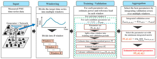
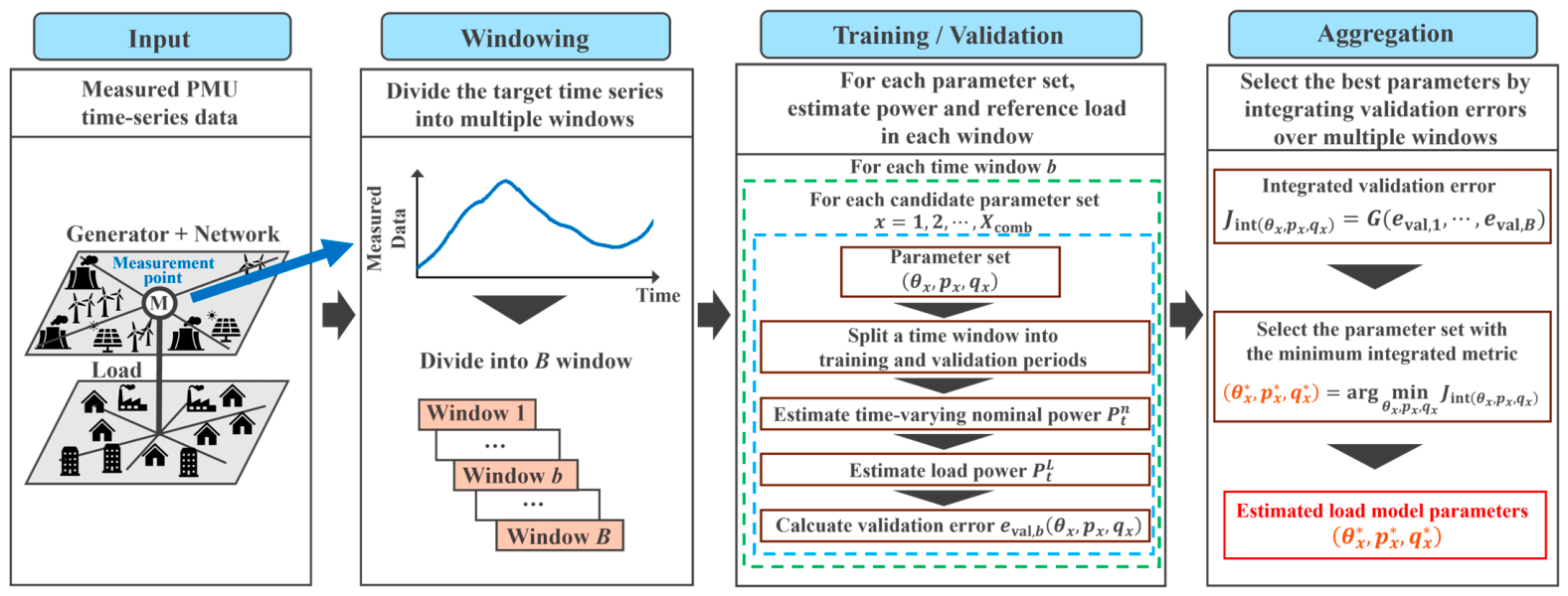
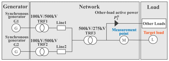
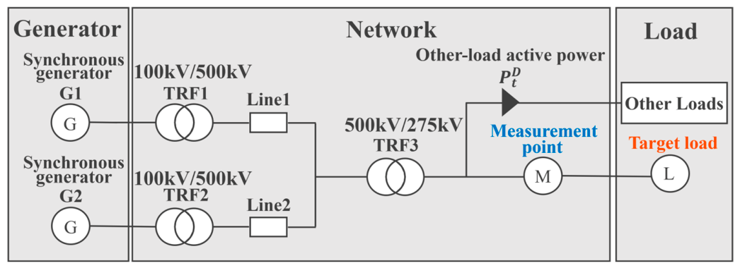
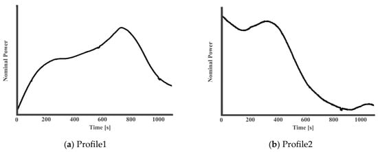
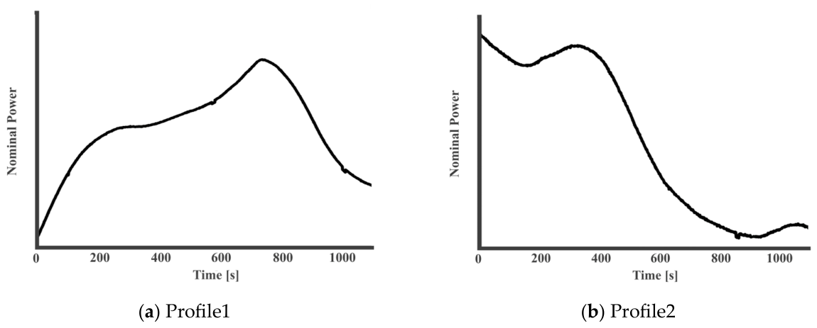
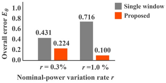
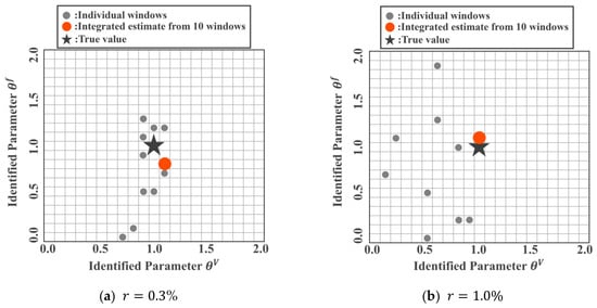
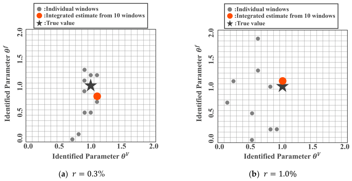
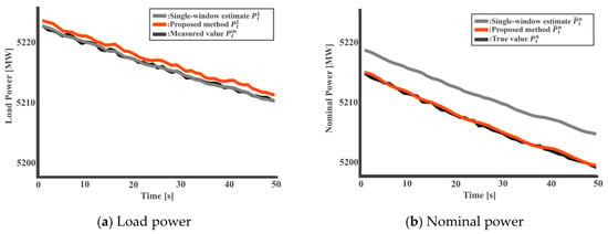
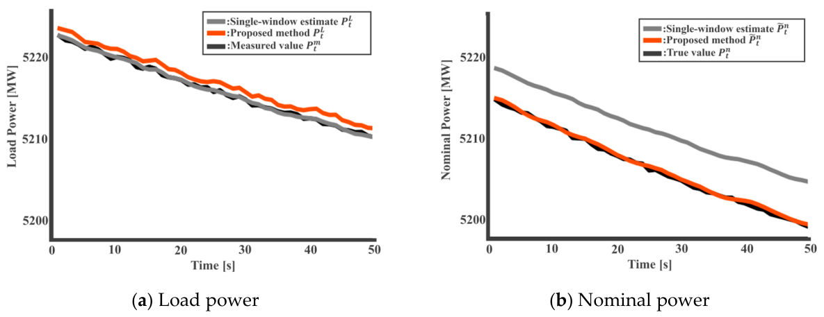
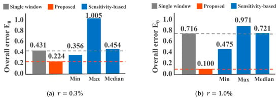
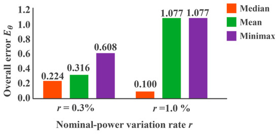
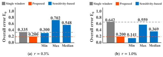
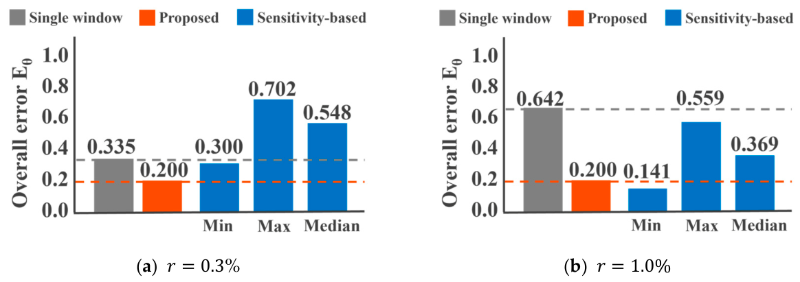
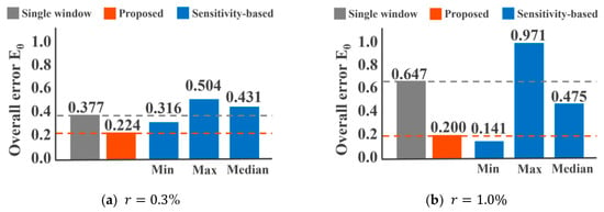
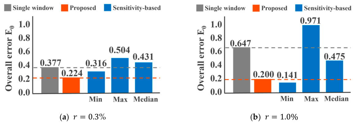
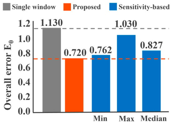
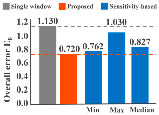
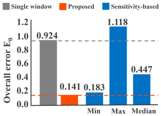
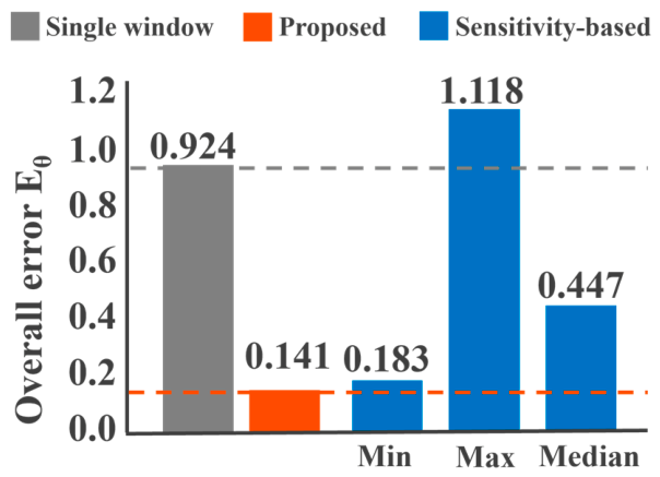

Disclaimer/Publisher’s Note: The statements, opinions and data contained in all publications are solely those of the individual author(s) and contributor(s) and not of MDPI and/or the editor(s). MDPI and/or the editor(s) disclaim responsibility for any injury to people or property resulting from any ideas, methods, instructions or products referred to in the content. |
© 2026 by the authors. Licensee MDPI, Basel, Switzerland. This article is an open access article distributed under the terms and conditions of the Creative Commons Attribution (CC BY) license.