


Abstract
Whether hydrogen should be delivered by pipeline or by truck is a large and largely irreversible investment decision. The cost information needed for this decision varies by a factor of several across the literature, and conventional single-value comparisons can reverse their conclusions depending on which value is selected. This study introduces a risk classification framework from construction management to define cost uncertainty as probability distributions grounded in the literature and in Korean empirical records. Four delivery modes were compared, specifically new pipelines, repurposed pipelines, high-pressure tube trailers, and liquefied hydrogen tanker trucks. Their twenty-year total costs were computed by Monte Carlo simulation with 20,000 draws for each combination of transport distance (10–500 km) and annual demand (1000–1,000,000 t/yr). The results are summarized as robustness maps that display only the mode with the lowest cost in at least 80% of the 20,000 cost scenarios. The synthesized cost distributions are consistent with the Korean cost records available for comparison, one of which was reserved from the model inputs. Where a repurposable pipeline exists, repurposing is effectively the only robust choice. In new corridors, new pipelines become robustly justified from 19,191 t/yr at the reference distance of 150 km, below which lies a gray band where assumptions decide the outcome. The viability of liquefied hydrogen delivery is determined not by technology but by who bears the liquefaction plant cost, and this boundary alone raises the share of the map on which liquefied hydrogen delivery is robust from 1% to 72.4%. The effective levers that advance the transition to pipelines are the operation and maintenance (O&M) rate (45.8%), the planning horizon (38.3%), and demand commitment (23.2%) rather than the carbon price (2.2%). Four announced Korean plans are located on the map in positions consistent with their project stages, which indicates that the framework can serve as a planning-stage diagnostic tool.
1. Introduction
Clean hydrogen has become a core energy carrier in the carbon neutrality strategies of many countries [1]. Accordingly, the delivery infrastructure that links production and demand sites has emerged as a decisive element of deployment. Delivery accounts for a substantial share of the delivered cost of hydrogen [2,3], and the structure of that cost depends on how the hydrogen is moved. Europe is advancing a continental hydrogen pipeline network built around the conversion of existing natural gas lines [4]. Korea has likewise announced a staged sequence of plans, from small pilot city networks to industrial corridors and long trunk lines [5,6,7,8,9,10]. Such infrastructure is difficult to reverse once built. The choice of delivery mode therefore locks in the cost structure of a hydrogen economy for decades, well beyond the horizon of any individual project.
The economic comparisons that should inform this choice have, however, reached diverging conclusions [3,11,12,13,14,15]. There is broad agreement that the relative advantage of pipelines and vehicle delivery shifts with distance and demand, yet the location of the boundary between them has remained dependent on study-specific assumptions. The state of the data lies behind this dependence. Key inputs such as pipeline unit costs, construction cost overrun, and maintenance rates vary by a factor of several across the literature. The annual pipeline operation and maintenance (O&M) rate is one example. Institutional sources report 0.8 to 1.7% of capital cost per year, whereas academic studies report up to 5%, a span of more than a factor of six. A conventional techno-economic analysis fixes one value from this span. Opposite conclusions can therefore be produced for identical conditions depending on the value selected, and the sensitivity of the conclusion is not visible in the result. From the standpoint of a decision maker, the issue is less which study to trust than that single-value comparison is difficult to accept as a sufficient basis for irreversible investment.
A review of existing approaches locates the gap. Classical comparative studies mapped the advantage regions of each mode on the distance and demand plane [2,3], and their intuitive maps are still consulted today. Their calculations are deterministic, however, and input uncertainty does not propagate to the result. Later studies that introduced probabilistic techniques made uncertainty explicit [16,17]. Yet the evidential basis of their distributions often rested on researcher judgment, and cases that added a validation step against measured records have been rare. Construction management, meanwhile, has accumulated a tradition of risk breakdown structures (RBS) and large-sample empirical analyses of cost overrun [18,19,20,21,22]. To the best of our knowledge, this asset has not been combined with the comparative economics of hydrogen delivery. The intuition of the map, the rigor of probability, and the empirical record of construction risk have thus developed in separate lineages without meeting in a single framework. That combination is precisely what this study attempts.
To this end, the study reframes the question. Instead of asking which mode is optimal, it asks from which combinations of distance and demand the choice remains unchanged however costs are realized. Four modes are compared, specifically new hydrogen pipelines, repurposed natural gas pipelines, high-pressure tube trailers, and liquefied hydrogen (LH2) tanker trucks. The comparison spans a grid of 10–500 km in transport distance and 1000–1,000,000 t/yr in annual demand. A probabilistic cost model couples mode-specific work breakdown structures (WBS) with a common RBS quantified by literature-based probability distributions. Monte Carlo simulation (MCS) then generates the total cost distribution of each mode at every grid condition. The result is summarized as a robustness map that displays only the modes whose win rate meets an 80% criterion. Whether the synthesized distributions contradict reality is examined for consistency against Korean empirical records. A separate robustness examination further shows that the conclusions are not driven by the methodological choices of the authors.
The contributions are threefold. First, a common RBS is introduced into delivery mode comparison, which structurally secures the fairness of the comparison across modes. Second, the evidential basis of the probabilistic inputs is made transparent through a semi-systematic literature harvest, calibration to Korean records, and an empirical consistency examination that separates the single record reserved from the inputs from the checks that reuse them. Third, win-rate-based robustness maps yield conditional prescriptions. These comprise a repurposing-first principle, a justification threshold for new pipelines, the dependence of LH2 delivery on a cost attribution boundary, and the institutional conditions that govern the transition to pipelines. The readability of the maps is illustrated with announced Korean plans. The valid range of the analysis is the regional scale of Korea, within 500 km, while the framework itself is designed to transfer to other countries and corridors by replacing region-specific parameters.
The remainder of this paper is organized as follows: Section 2 documents the literature harvest procedure, establishes the cost structures of the modes and the common RBS, and discloses the distributions and sources of all quantified factors. Section 3 formalizes the cost model, the MCS procedure, the validation design, and the robustness criterion. Section 4 reports the consistency checks, the robustness maps, the effect of the liquefaction cost boundary, the methodological robustness examination, and the placement of Korean plans. Section 5 positions the results against the literature, interprets the sensitivity of the robust frontier, and discusses policy implications. Section 6 concludes with limitations and future work.
2. Literature-Based Risk Structure
2.1. Semi-Systematic Literature Harvest
The credibility of a probabilistic cost comparison rests on the evidence behind its input distributions. The literature review in this section was therefore designed not as a survey of research trends but as a transparent procedure for constructing model inputs. Because pre-registration and independent dual screening were not applied, the procedure is described as semi-systematic rather than as a formal systematic review. Only the elements essential to the present purpose were retained, namely explicit search sources, pre-declared inclusion criteria, and a documented harvesting record.
Three families of sources were searched in parallel. These comprised institutional reports, peer-reviewed academic studies [3,11], and Korean government documents together with records from demonstration projects. The institutional reports came from the European Hydrogen Backbone (EHB) initiative, the International Energy Agency, laboratories of the United States Department of Energy, and the EU Agency for the Cooperation of Energy Regulators [1,2,4,23]. As an inclusion criterion, at least three mutually independent sources were required for each probabilistic factor. For the four factors that dominate the results, that is, the new pipeline unit cost, construction cost overrun, pipeline operation and maintenance (O&M) rate, and vehicle system costs, at least five sources were required. Harvesting proceeded through three general rounds and one targeted round that addressed the remaining gaps. A second targeted round was subsequently added for three areas in which the earlier rounds yielded thin coverage, specifically contractual structures for midstream energy assets, cost escalation in brownfield and retrofit works, and recent techno-economic assessments of hydrogen delivery.
Approximately sixty unique documents were adopted in total. A notable feature of the harvest is the wide dispersion of reported values for identical factors. For the annual pipeline O&M rate, institutional sources report 0.8 to 1.7% of capital expenditure [4], whereas academic studies report values up to 5% [3,11], a span of more than a factor of six. This study interprets such dispersion not as a defect of the data but as evidence that single-value comparison cannot be conclusive. The full span is therefore carried into the analysis as probability distributions.
2.2. Cost Structures of the Delivery Modes
A mature consensus already exists on what generates cost in each delivery mode. Pipeline delivery decomposes into line capital expenditure governed by diameter and length, compression equipment and its electricity, and maintenance expenses proportional to the invested capital [1,3,4,24,25]. Vehicle delivery consists of the capital and replacement of the fleet required to serve the demand, together with driver labor, fuel, and maintenance [2,3,26,27]. The liquefied hydrogen (LH2) chain adds the liquefaction plant, its electricity demand, and boil-off losses during storage and transfer [12,28]. Repurposing an existing natural gas pipeline is conventionally treated as a fraction of the corresponding new-build cost [11,23,29,30,31,32].
For Korean conditions, this cost skeleton can be confirmed at the level of actual contract documents. This study employed a unit cost platform built from itemized Korean construction contracts, which verifies the composition and magnitude of cost items from earthwork and road restoration to main line installation and mechanical equipment. Section 3 formalizes this decomposition as the work breakdown structure (WBS) of each mode. The WBS of this study is therefore not a new invention but an organized form of the cost skeleton shared by the literature and by Korean contract practice.
Where the literature diverges is not in the composition of cost but in the uncertainty of its magnitude. Reported values differ substantially between studies, and the drivers of variation differ across modes. Line capital costs respond to ground conditions and urban routing, whereas vehicle costs respond to equipment markets and technological maturity. Fair comparison therefore hinges on a systematic classification of the causes of cost variation rather than on a longer list of cost items. This motivates the risk breakdown structure introduced in the next subsection.
2.3. Common Risk Breakdown Structure and Mode Applicability
An economic comparison across delivery modes is fair only when every mode is examined against the same set of risks. If uncertainty items are assigned to each mode in an ad hoc manner, the outcome of the comparison is determined by the selection of items rather than by the calculation. The risk breakdown structure (RBS) has long been established in construction management as a hierarchical instrument for organizing project risk [18,19,20,21]. To the best of our knowledge, however, no published study has applied a common RBS to the comparative economics of hydrogen delivery modes. This combination constitutes the first contribution of the present study.
The common RBS constructed here consists of seventeen nodes in five categories. Category R1 (market and price) covers steel and material prices, the construction cost index, exchange rates, and equipment market prices. Category R2 (design and specification) addresses diameter and pressure specifications, the hydrogen-specific code premium, and the condition of existing lines. Category R3 (construction and site) contains ground conditions, urban routing, construction methods, and construction cost overrun, while category R4 (institutional and social) covers permitting, right of way, public acceptance, and safety regulation. Category R5 (procurement and technology) captures economies of scale and technology learning. The nodes were compiled from factors reported in the literature as causes of cost variation and were refined for mutual exclusivity.
The intensity with which each node enters the cost calculation of each mode was rated on a five-level scale. The levels are Quantified for direct inclusion as a probability distribution, Partial for partial or scenario-based inclusion, Minor for treatment as a fixed value, Qualitative for a qualitative rating only, and Not applicable for structural irrelevance. Two criteria governed the rating: the availability of quantitative evidence and the materiality of the node for the cost of the mode concerned. The resulting applicability matrix is presented in Table 1, and the evidence behind each rating is linked to Table 2. Pre-declaring the rating criteria is a safeguard against arbitrariness in the construction of the matrix.
Table 1.
Common risk breakdown structure and mode applicability matrix.
Table 2.
Probability distributions, parameters, and sources for all quantified factors.
Table 1 reveals a structural asymmetry in the risk profiles of the modes. The Quantified ratings of the pipeline modes concentrate in categories R3 and R4, whereas those of the vehicle modes concentrate in R1 and R5. The economics of pipelines is governed by the capacity to manage site and institutional uncertainty, while the economics of vehicle delivery is governed by equipment markets and technological maturity. This asymmetry later emerges as the structural reason why the two families of modes exhibit cost distributions of different widths.
2.4. Probability Assignment
Probabilistic factors were assigned a program evaluation and review technique (PERT) distribution defined by the harvested minimum, mode, and maximum values. PERT is standard practice in construction risk analysis under sparse data and matches naturally with the three-point outputs of the literature harvest [19]. Three explicit exceptions were made. Construction cost overrun follows a shifted lognormal distribution to reproduce the strong right skew of the empirical record. Factors whose values move jointly, such as the high-pressure trailer configuration and the carbon price, are treated as scenario sets. The liquefaction plant cost combines a power law with a uniform uncertainty coefficient.
Construction cost overrun dominates the results and is therefore described in detail. An empirical analysis of 412 pipeline projects [22] reports an overrun distribution with a mean of +6.5%, a standard deviation of 33.5%, and a skewness of at least 2.2, the latter adopted as a conservative lower bound. Solving analytically for a shifted three-parameter lognormal distribution that reproduces these moments yields X = 0.5450 + LogN(mu = −0.8275, sigma = 0.5892). Verification with two million samples reproduced the target moments with a mean of 1.0651, a standard deviation of 0.3349, and a skewness of 2.22. The lower bound of 0.545 admits cost realizations down to approximately 46% below the estimate, and the 95th percentile corresponds to an overrun of +70%, which covers the extreme cases observed in the empirical record.
No overrun dataset for pipeline repurposing of a size comparable to the 412-project new-build sample is available, so the applicability of the new-build distribution to the repurposing branch cannot be established empirically. Renovation studies in the building sector nonetheless indicate that works on existing facilities carry unforeseen-condition risk that new construction does not [42,43]. Section 4.4 therefore assigns the repurposing branch a distinct risk profile, varied separately in location and in scale, and reports the departure from the new-build profile at which the mode ranking would change, without assuming any particular departure.
The distributions, parameters, and sources of all eighteen quantified factors are disclosed in Table 2, of which seventeen enter the calculation and one is defined but not applied. The rows of Table 2 are linked to the categories of Table 1 so that each Quantified rating can be traced to its implementing distribution. Factors that were defined and verified but deliberately excluded are also disclosed with their reasons. The construction cost index was derived from the official Korean statistical tables [36], yet it was not applied as a multiplier. Inflation effects are already embedded in the empirical overrun record, and applying the index again would double count them. Disclosing unused values is intended to demonstrate the transparency of input selection. Each factor enters Equations (1)–(4) at the position indicated by its work breakdown item: unit cost and overrun factors multiply the capital terms, rate factors multiply the recurring cost terms, and vehicle factors enter the trip count and fuel terms.
All unit costs are expressed on a direct construction cost basis, and exchange rates of 1380 KRW/USD and 1450 KRW/EUR were applied. Korean demonstration projects are anonymized for confidentiality, and each project retains the same designation, Project A through Project G, throughout the paper.
2.5. Calibration to Korean Conditions
Three anchors ground the internationally sourced distributions in Korean conditions. First, the three points of the 8 inch new-build unit cost were constructed from a unit cost platform based on actual Korean contract documents at seven levels of detail. Second, a Korean hydrogen pipeline demonstration project, Project D, provides as-built direct costs and operating records that anchor the unit cost distribution and the mode of the O&M rate. Third, the published unit cost of an urban pilot project, Project A, is stated on a total project cost basis that differs from the direct cost basis. It was therefore reserved exclusively for validation rather than used as an input (Section 4.1). Keeping data with different bases out of a shared role is the governing principle of the calibration.
Three points are stated regarding the transferability of the international evidence. The overrun record [22] derives mainly from oil and gas pipelines, so it was used exclusively as an input while validation relied on Korean empirical anchors. The mean overrun of Korean public infrastructure projects, reported at approximately +30% [37], was confirmed to lie within the adopted distribution. Hydrogen-specific cost increases are represented separately by the code premium node (R2.2), so no double counting with the overrun factor arises. Applying the same overrun distribution to repurposed pipelines is an approximation given their different work composition, and the wide upper bound of the retrofit ratio partially absorbs this uncertainty. Unit costs for the large diameters of 20 and 30 inch rest on European institutional sources and their interpolation [4], as no Korean empirical record yet exists at this scale.
3. Methods
3.1. Analytical Framework
The analytical procedure of this study consists of four stages, as presented in Figure 1. First, the cost structure of each delivery mode is decomposed by its WBS. The drivers of variation in each cost item are then coupled with the probability distributions of the common RBS constructed in Section 2. Second, MCS is performed for every condition on the distance and demand grid to yield the distribution of life-cycle total cost for each mode. Third, the synthesized distributions are compared against Korean empirical anchors to confirm consistency. Fourth, a robustness map is derived that displays only the modes satisfying a pre-defined win rate criterion. Fairness across modes is secured by the common RBS (Section 2.3), while the reliability of the inputs is secured by the harvest protocol (Section 2.1) and by the validation design (Section 3.5). This section concentrates on formalizing the calculation and introduces no new numerical values; all parameter values refer to Table 2 as their single source.
Figure 1.
Analytical framework of the study in four stages (Section 3.1).
3.2. Delivery Modes and System Boundaries
Four delivery modes are compared: new hydrogen pipelines (NP), repurposed natural gas pipelines (RP), high-pressure tube trailers at the 200 bar class (TT), and LH2 tanker trucks (LT). Repurposing is a conditional alternative that exists only where a convertible line lies along the corridor, so the robustness maps are presented separately for corridors with and without a repurposable line (Section 4.2). The system boundary is identical for all modes and extends from the production gate to the delivery gate. The evaluation horizon T is 20 years. The discount rate ρ is 4.5%, the standard rate of Korean public investment appraisal [44], with 8% as an alternative reflecting international practice [1,2]. Demand is assumed constant over the horizon, and the effect of gradually increasing demand is examined separately in the condition sensitivity analysis (Section 5.2). The valid range of the analysis is the regional scale of Korea, within 500 km, and social costs, public acceptance, and natural gas blending lie outside the scope of this study.
The LH2 mode requires one additional boundary definition. When the carrier receives gaseous hydrogen and performs liquefaction itself, the liquefaction plant investment and the liquefaction electricity belong inside the delivery cost. When the carrier purchases hydrogen that is already liquefied and only transports it, both items fall outside the boundary. Both contract structures exist in real markets, so selecting either one would be arbitrary. This study therefore analyzes the two boundaries in parallel and quantifies the difference between them (Section 4.3).
Throughout this study, L denotes the routed length of the delivery corridor rather than the straight-line separation of the production and demand sites, and the distances used for the Korean projects in Section 4.5 are the planned route lengths stated in public announcements. Siting and routing constraints arising from existing infrastructure, land use and terrain therefore enter the analysis through the routed length and through the right of way and site condition factors of Table 2. The analysis does not evaluate route feasibility or select an alignment. A corridor is assumed to be realizable, and the map then determines which delivery mode is robust for its length and demand. Where a corridor traverses terrain that materially exceeds the range of the site condition factors, corridor-specific estimation should replace the map reading.
3.3. Cost Model
3.3.1. Common Structure
The life-cycle total cost of mode m ∈ {NP, RP, TT, LT} is defined as the sum of capital expenditure and discounted operating expenditure.
Each component of capital and operating expenditure is computed by the multiplicative structure Bm,k·Πj(1 + rj). Here, Bm,k denotes the base cost of the k-th WBS item of mode m. The factors rj are the RBS risks applied to that item, drawn from the distributions of Table 2. Separating base costs from risk multipliers serves two purposes. It structurally prevents double counting and omission among risk factors, and it allows sensitivity analysis to attribute cost variation to individual RBS nodes. The correspondence among WBS items, risk factors, and parameters is presented in Table 3.
Cm = CAPEXm + Σt=1T OPEXm,t (1 + ρ)−t
Table 3.
Mode-specific work breakdown structures and their links to risk factors and parameters.
3.3.2. Pipeline Modes
The capital expenditure of a new pipeline consists of line construction and the compressor station.
Here cL(d) is the direct construction cost per unit length at diameter d, L is the transport distance, and Xov is the construction cost overrun multiplier (shifted lognormal, Section 2.4). The share xrow covers right of way, and γind is the indirect and engineering coefficient. The compressor station investment is the product of a unit cost ucs and the required rating Pcs, which follows from demand and from compression energy proportional to distance. For the repurposed mode, the line cost is the same-diameter new-build cost multiplied by the retrofit ratio xretro, and the compressor station is added identically. Annual operating expenditure comprises the O&M rate applied to the invested line capital, compression electricity proportional to distance, and the carbon cost given by the emission factor and the carbon price path.
CAPEXNP = cL(d)·L·Xov·(1 + xrow)·γind + ucs·Pcs
3.3.3. Vehicle Modes
Vehicle cost estimation begins with fleet sizing. The required fleet N is the annual demand divided by the annual delivery capability of one vehicle. That capability is the product of the effective payload weff and the feasible number of annual round trips ntrip(L).
Here Hop is the annual operating time, is the average speed, and τhand is the loading and unloading time. The adopted values were Hop = 3600 h per year (12 h per day over 300 operating days), = 55 km/h, and τhand = 2 h. Vehicle capital is annualized with the capital recovery factor (CRF) over the replacement cycle nrep, eight years for high-pressure vessels and twelve years for tankers. This annualization keeps the comparison with pipelines undistorted by the length of the horizon. The annual capital charge is Aveh = Pveh·N·CRF(ρ, nrep) with the standard definition CRF(ρ, n) = ρ(1 + ρ)n/[(1 + ρ)n − 1]. Operating expenditure comprises driver labor, fuel, maintenance, refueling electricity, and carbon cost, in the same form as the pipeline case. For the LH2 mode, the cost attribution boundary of Section 3.2 determines whether the liquefaction plant and its electricity are included. The plant investment follows a power law in daily capacity S, written as CLP = a·Sb·ξ with b < 1 and an uncertainty coefficient ξ. The functional form and the scale exponent are adopted from the United States Department of Energy cost model family [2]. Mass losses along the LH2 chain are reflected as an upward correction of the quantity that must be transported to meet the delivered demand.
The effective payload of a 200 bar tube trailer is drawn from a PERT distribution over 198, 250 and 300 kg of hydrogen per trip, and a higher-pressure trailer set of 373 to 500 kg is treated as a scenario variant. The liquefied hydrogen tanker carries 3000 kg of hydrogen per trip, with a 3% chain loss applied as an upward correction of the quantity that must be transported to meet the delivered demand. Both vehicle types are diesel powered. Fuel cost is charged over the round trip distance, and the resulting carbon dioxide emissions are priced through the emission factors and the carbon price path of Table 2.
3.3.4. Diameter Assignment
Pipeline diameter is not a fixed input but is determined endogenously by demand and distance. The diameter is assigned as the smallest member of the candidate set whose transport capacity limit meets the demand.
The capacity limit was computed as a function of distance with the general flow equation for isothermal compressible flow [45]. The computation assumes an inlet pressure of approximately 50 bar and a delivery pressure of 30 bar. Internal diameters are obtained from X70 steel with wall thickness deducted, and for the 12 and 16 inch tiers the wall thickness is interpolated between the 8 and 20 inch entries, giving 305.8 and 386.9 mm. Their unit cost distributions are PERT with points of 1282, 1525 and 2269 million KRW per km for the 12 inch class and 1661, 1862 and 2455 for the 16 inch class, interpolated between the 8 and 20 inch entries of Table 2, and their cost samples are generated by the same procedure as for the original tiers. The functional form, detailed assumptions, capacity tables, and a cross-check against published European capacity figures are provided in Appendix A. Compression cost is charged in proportion to distance, whereas the hydraulic calculation assumes a single pressure section without intermediate boosting. The design alternative this assumption excludes, namely adding intermediate compression instead of enlarging or paralleling the line, is an established option in the repurposing literature [29], and the sensitivity of the long-distance threshold to the capacity assumption is reported in Section 4.4. This simplification charges pipelines for recompression without crediting its capacity recovery, so it acts against the pipeline modes and renders the thresholds of this study conservative. Its quantitative effect is examined through the ±25% capacity variants in Section 4.4.
3.4. Monte Carlo Simulation
The computational grid spans 10–500 km in transport distance and 1000–1,000,000 t/yr in annual demand at logarithmic spacing. At each grid condition, risk factors were drawn 20,000 times from the distributions of Table 2 and the mode costs were computed by Equations (1)–(4). The random seed was fixed at 42 so that every result is reproducible. In the base analysis, the factors are drawn independently. Pairs such as the unit cost and the cost overrun may plausibly be positively correlated. Correlated variants are therefore included in the robustness examination of Section 4.4, where the effects of sample size and seed selection are also reported.
The Python (version 3.11) code that implements Equations (1)–(6) and the Monte Carlo procedure was written with the assistance of a generative AI tool, Claude Opus 5 (Anthropic), which was also used to develop and refine the figures. All model logic, input parameters, numerical results, and figure contents were verified by the authors.
3.5. Validation Design
The empirical source of the overrun distribution [22] enters the model as an input, so reusing the same data to confirm the model would constitute circular reasoning. The examination design therefore separates records by the role they play. Records that entered the construction of the inputs can support an internal check only, whereas a record reserved from the inputs can support an external one, and Section 4.1 reports the two classes separately rather than presenting them as a single validation.
Three anchors are used, all of them Korean records. The first is the extent to which the synthesized cost distribution covers the estimation range of the Korean itemized cost platform. The second and third are the percentile positions of the unit costs of Project D and of Project A within the synthesized distribution. Of these, the platform and Project D entered the construction of the inputs, so their agreement is internal and establishes only that the synthesized distribution reproduces its own inputs, whereas Project A was reserved from the inputs and provides the single external check. Table 4 additionally reports the agreement between the simulated mean overrun and the empirical average of the sample to which the overrun distribution was calibrated, which is an implementation check on the calibration rather than an anchor. This examination is a consistency check that confirms the absence of contradiction with observable reality rather than a statistical goodness-of-fit test. Its nature and limits are stated together with the results in Section 4.1.
Table 4.
Summary of the consistency examination against Korean records.
3.6. Robustness Criterion and Sensitivity Plan
At each grid condition (L, Q), the win rate of mode m is defined as the fraction of the 20,000 cost realizations in which that mode attains the lowest cost.
A condition is colored as the robust region of a mode when the leading win rate reaches 80%. Conditions where no mode reaches the criterion are marked as assumption-dominated. The latter does not indicate that judgment is impossible; it indicates that the input assumptions decide the outcome there, so acquiring further information should precede any commitment. The topology of the map is preserved when the criterion is changed to 70% or 90% (Section 4.4). The pipeline justification threshold Q* is defined as the smallest demand at which the win rate of the new pipeline reaches and sustains the criterion as demand increases at a fixed distance.
Because the win rate can vary non-monotonically near diameter transitions, Equation (6) requires the first sustained crossing rather than a momentary one. Numerically, the crossing is located on a scan whose resolution is fine enough to resolve the win rate at every diameter transition, and bisection then refines it to a relative error of 0.5%. A coarse scan is not sufficient for this purpose, because the win rate variation induced by a diameter transition spans a demand ratio of approximately 1.2 to 1.5 and can fall between successive nodes of a coarser grid.
wm(L, Q) = (1/Nsim)Σi1{Cm(i) = minm′ Cm′(i)}
Q*(L) = min{Q:wNP(L, Q′) ≥ 0.8, ∀Q′ ≥ Q}
The sensitivity analyses were designed in advance as three layers with distinct questions. The first layer asks whether the results depend on the methodological choices of the authors, including distribution shapes, tail thickness, correlation, seeds, and the diameter assignment. This concerns the reliability of the map itself and is examined in Section 4.4. The remaining layers concern interpretation and are discussed in Section 5.2. One measures the influence of individual input factors on the threshold. The other measures the influence of policy-determined conditions, specifically the O&M level, the planning horizon, the carbon price, and the speed of demand build-up.
4. Results
4.1. Consistency Check of the Synthesized Distributions
The results of the three-anchor examination designed in Section 3.5 are presented in Figure 2 and Table 4. The synthesized distribution of the 8 inch new-build unit cost covers 80.2% of the estimation range of the Korean itemized cost platform. The as-built unit costs of the two Korean projects fall within the body of the corresponding synthesized distributions. Project D lies at the 24th percentile on a direct cost basis, and Project A at the 42nd percentile on a published total cost basis. The simulated mean overrun of 6.5% equals the empirical average of the 412-project sample to which the overrun distribution was calibrated [22], and this agreement confirms that the calibration was implemented correctly. It does not validate the distributional assumption. It remains below the average of 11% reported for compressor station construction [38].
Figure 2.
Synthesized unit cost distributions and Korean empirical anchors. (a) As-built direct cost of Project D (24th percentile). (b) Published total cost of Project A (42nd percentile).
The essential observation is that both as-built values sit in the body of the distribution rather than in its tails. Had the synthesized distribution been systematically inflated, the as-built values would have been pushed toward its lower tail, and the opposite bias would have pushed them upward. The observed percentile positions support the absence of a contradiction with the observed records in either direction.
The three checks do not carry equal evidential weight. The platform coverage and the percentile position of Project D are internal, because both records entered the construction of the unit cost distribution (Table 2), so what they establish is that the synthesized distribution reproduces its own inputs. The only record reserved from the inputs is Project A. The examination should therefore be read as a check for contradiction with observable Korean outcomes, resting on one independent record, and not as a statistical test of fit. Establishing distributional adequacy would require an as-built sample that does not yet exist for Korean hydrogen pipelines, and Section 5.3 identifies the accumulation of such records as the highest-value information investment available.
The limits of this examination are stated explicitly. Two anchor projects cannot support a statistical test of distributional shape, and the examination is a consistency check in the sense defined in Section 3.5. Full separation of the input and examination sources holds only for Project A. The remaining two checks reuse records that entered the inputs and are therefore reported as internal consistency checks.
4.2. Robustness Maps
Figure 3 presents the central result of this study, the robustness maps for a corridor with a repurposable pipeline (a) and for a new corridor (b). The color of each cell indicates the mode whose win rate, Equation (5), reaches 80%, and cells where no mode reaches the criterion are shown in gray as assumption-dominated. The dotted curves are the capacity limits of the 8 and 20 inch diameters under the assignment rule of Equation (4). The dashed curve is the capacity limit of a single 30 inch line; the area above it would require parallel lines or larger diameters.
Figure 3.
Robustness maps of least-cost delivery modes: (a) corridor with a repurposable natural gas pipeline; (b) new hydrogen corridor. Gray cells are assumption-dominated.
In the repurposable corridor (a), repurposing satisfies the robustness criterion in 162 of the 196 conditions (83%). The robust region of the tube trailer is confined to 13 conditions (7%) in the shortest-distance, lowest-demand corner, and the remaining 21 conditions (11%) are assumption-dominated. Notably, not a single condition makes the new pipeline robust. Repurposing delivers the same transport capability at 10–50% of the new-build capital cost. Under that ratio, no combination of distance and demand within the analyzed range allows a new line to beat a convertible existing one with confidence. This result is consistent with the European strategy that places the conversion of existing gas networks at the core of hydrogen infrastructure [4,23]. It quantitatively supports treating repurposing screening as the first question of any hydrogen delivery plan.
In the new corridor (b), the new pipeline dominates 125 conditions (64%) and the tube trailer 48 conditions (24%), separated by a diagonal gray band of 21 conditions (11%). The robust region of the LH2 tanker truck is limited to 2 conditions in the longest-distance, low-demand corner, and its extreme sensitivity to the cost attribution boundary is examined in Section 4.3. Following the 150 km column from low to high demand reveals the structure of the transition. The tube trailer sustains a win rate of 98% or higher up to approximately 8400 t/yr. The leading win rate then collapses to 51% near 14,000 t/yr, and the new pipeline recovers the criterion with 92% at approximately 24,000 t/yr. Refining this interval by Equation (6) yields the justification threshold of 19,191 t/yr.
The threshold increases monotonically with distance. Under the reference conditions it rises gradually, from approximately 11,000 t/yr at 50 km to 16,000 t/yr at 100 km and 21,000 t/yr at 200 km. It then rises to approximately 31,000 t/yr at 300 km. The gradual segment reflects the ordinary contest between the distance-proportional cost structure of trucking and the largely fixed capital structure of pipelines. The rise near 300 km has a physical origin: the closing of the 8 inch transport window, which forces a step to a larger diameter class and raises the capital cost stepwise. The same mechanism explains why the dotted capacity limits in Figure 3 slope downward with distance.
The dotted curves inside the blue region further partition the robust pipeline area by diameter class. Conditions below the 8 inch limit correspond to 8 inch projects, those between the two dotted curves to the 12, 16 and 20 inch classes, and those above to the 30 inch class. The capacity limits of the 12 and 16 inch tiers are omitted from the figure for legibility and are listed in Table A2. No Korean plan examined in Section 4.5 lies above the single 30 inch limit. The diameter partition extends the reading of the map from mode selection to the scale of the required capital commitment.
The gray band itself carries information. A single-value analysis is forced to output a winner even inside this band, and which side wins is decided by the values selected. A substantial share of the conditions treated by previous studies falls in or near this band. The band therefore offers a structural explanation for the divergence of published conclusions, a point developed in Section 5.1.
4.3. Effect of the Liquefaction Cost Attribution Boundary
Figure 4 shows how the two cost attribution boundaries defined in Section 3.2 reshape the new-corridor map. The two panels differ in exactly one assumption, the inclusion or exclusion of the liquefaction plant investment and the liquefaction electricity, and panel (a) coincides with the reference map of Figure 3b.
Figure 4.
Effect of the liquefaction cost attribution boundary on the new-corridor map: (a) liquefaction plant and electricity inside the boundary; (b) excluded.
The contrast is stark. When liquefaction costs lie inside the boundary (a), the robust region of the LH2 tanker truck consists of 2 conditions at the longest distances. Carrying the plant investment and an electricity demand of 9–15 kWh per kilogram, the mode prevails only where trucking numbers explode for its competitor. When the carrier instead purchases hydrogen that is already liquefied (b), the reallocation is sweeping. The LH2 tanker truck dominates 142 of the 196 conditions (72.4%), the robust region of the tube trailer disappears entirely, and the new pipeline retreats to 38 high-demand conditions (19%). The structural advantage of a tanker payload roughly ten times that of a 200 bar tube trailer had been masked by the attribution of the pretreatment cost.
These results suggest that the divergent published assessments of LH2 delivery economics may originate in boundary definitions rather than in technology. Both boundaries correspond to real contract structures, so this study does not select one as correct; the policy reading of this result is developed in Section 5.3.
4.4. Robustness to Methodological Choices
Table 5 reports whether the results depend on the methodological choices of the authors. Alternative choices were applied along six axes, specifically distribution shape, overrun tail thickness, factor correlation, random seed, ladder configuration, and capacity bounds. The shift in the threshold at the 150 km reference distance was measured for each. All variants were recomputed under the five-tier reference specification of Section 3.3.4. The table baseline is the reference threshold of 19,191 t/yr, and the 300 km rows are reported against the 300 km reference of 30,553 t/yr.
Table 5.
Sensitivity of the justification threshold to methodological variants.
The influence of methodological choices remains between −4.5% and +12.8%, apart from the deliberately coarsened two-tier ladder. The largest variant replaces PERT with a triangular distribution (+12.8%). The triangular form assigns thicker tails to the same three points, widens the cost dispersion of the pipeline, and thereby delays the attainment of the win rate criterion. Imposing correlation between the unit cost and the overrun (+3.6% and +6.9%) acts in the same direction, because positive correlation synchronizes adverse cost realizations and thickens the upper tail. The skewness variants of the overrun act in both directions with small magnitudes (+3.1%, −4.5%). The seed variants (±0.7%) and the capacity variants at the reference distance (0.0%) are immaterial. Removing the intermediate 12 and 16 inch tiers leaves the reference threshold unchanged, whereas collapsing the ladder to two tiers raises it by 136.2%, which quantifies the contribution of the 20 inch tier. Changing the decision criterion reshapes the map only gradually. At 70% and 90% the colored share becomes 94% and 85%, the ordering structure holds at every distance, and the threshold moves to 17,133 t/yr (−10.7%) and 22,792 t/yr (+18.8%). This movement exceeds the method variants but differs in kind, because the criterion is not an estimation choice but the confidence level selected by the decision maker. This study reports the conservative level of 80%, four futures out of five, as the default and states the alternatives alongside. Overall, the methodological effects are one order of magnitude smaller than the condition effects reported in Section 5.2. This supports the reading that the conclusions derive from the data rather than from the method.
The single exception concerns long distances. At 300 km, removing the intermediate 12 and 16 inch tiers raises the threshold by 37.0%, reducing the ladder to two tiers raises it by 86.7%, and relaxing the capacity bounds by 25% lowers it by 21.1%. Long-distance thresholds therefore depend directly on transport capacity assumptions. Combined with the single pressure section assumption of Section 3.3.4, this dependence delimits the valid range of the map and indicates that corridor-specific pressure and diameter design should precede judgments on long-distance projects.
The risk assignment of Section 2.4 raises a further question. Does the first conclusion of this study survive a repurposing risk profile that differs from the new-build profile? Table 6 reports the result. With the repurposing overrun mean raised 15% and 30% above the new-build mean at a preserved coefficient of variation, the repurposing-robust region contracts only from 162 to 158 and 156 of the 196 grid conditions, and widening the dispersion of the repurposing overrun by factors of 1.5 and 2.0 at a preserved median yields 160 and 156 conditions. The departure must become far larger before the conclusion changes. At a mean 3.25 times the new-build mean, repurposing still holds 127 conditions, and beyond approximately 3.5 times its robust region is absorbed into the assumption-dominated band, and it does not pass to the new pipeline, which stays below the criterion at every condition in this range. The mechanism is structural. Repurposing capital expenditure is 10 to 50% of new construction for the same diameter (Table 2), so an overrun premium must approach a factor of four before it can close that gap. The practical reading is that a higher retrofit risk does not reverse the repurposing-first prescription but widens the region in which corridor-specific investigation of the existing line, in particular its integrity records and pressure history, must precede commitment.
Table 6.
Robustness of the repurposing-first conclusion to a distinct repurposing overrun risk profile.
4.5. Placement of Announced Korean Plans
Figure 5 places four announced Korean hydrogen delivery plans on the new-corridor map, using coordinates estimated from public announcements [5,6,7,8,9,10]. The coordinates are indicative estimates (est.), and the projects are anonymized. The published production capacity of Project A falls below the demand axis of the map. The project was therefore placed at the axis floor of 1000 t/yr, and this placement was confirmed not to affect the reading.
Figure 5.
Announced Korean hydrogen plans (anonymized) overlaid on the new-corridor robustness map. Marker positions are indicative estimates from public announcements.
The two pilot-scale projects, Project A and Project P, occupy short-distance, low-demand positions across the tube trailer region and the lower edge of the gray band. This placement matches current practice, in which pilot projects begin with truck delivery, and it also yields a dynamic reading of their future course. The transition points are strongly distance-dependent. At the trunk-line scale the threshold is on the order of 20,000 t/yr. For 10 km corridors, however, the transition begins at approximately 2000–3000 t/yr, and for 15 km corridors at approximately 3000–5000 t/yr. Both pilot projects would therefore enter the reassessment zone after only modest demand growth, and the present scale of Project P already sits near its entrance.
The readings of the two large projects gain precision when combined with the diameter partition. Project S settles in the interior of the robust pipeline region, with a demand far below the 8 inch capacity limit at its distance, and thus reads as an 8 inch class project. Project G also lies in the robust pipeline region, at approximately 83% of the 20 inch capacity limit at its distance, near the boundary of the 30 inch class. Because long-distance diameter boundaries are sensitive to capacity assumptions (Section 4.4), the diameter decision of this project reads as a matter requiring corridor-specific pressure system design rather than map-level judgment. None of the four plans lies above the single 30 inch limit.
The estimated nature of the coordinates is a limitation of this placement, yet its consequences differ by project. Projects A, P, and S sit in the interiors of their regions, so their readings are insensitive to moderate coordinate errors. Project G sits near a class boundary, and coordinate uncertainty propagates directly to its diameter reading. The limitation thus functions as information, identifying for which project a precise coordinate determination is the priority.
The purpose of this subsection is to confirm that the map functions as a reading instrument for real plans, not to evaluate the feasibility of individual projects. The four placements are consistent with the direction of the announced national plans. For plans in or approaching the gray band, the map further identifies the assumptions to be narrowed before commitment, in particular measured O&M records and long-term demand commitment. The map can therefore serve as a planning-stage diagnostic tool.
5. Discussion
5.1. Position Against the Literature
The maps of this study allow the diverging conclusions of the delivery mode literature [3,11,12,13] to be reinterpreted consistently on a single coordinate plane. Conditions for which pipeline advantages have been reported correspond broadly to the high-demand region of the map, and conditions favoring vehicles correspond to the low-demand region. A substantial share of the contested conditions lies in or near the gray band. A single-value analysis must output a winner even inside this band. The divergence of the literature is therefore understood not as a defect of individual studies but as an intrinsic property of that band. Assumptions decide the outcome there, and different studies selected different assumptions.
Within this frame, the findings of previous studies and the present maps support one another. The crossover structure of the classical mode comparison [3,24] agrees in direction with the region ordering of the map. The reported economics of pipeline repurposing [11,14,15] is consistent with the repurposing-dominated panel of Figure 3a. The finding that trailer specifications govern vehicle competitiveness [26,27] is absorbed into this framework through the vehicle-side factors in the tornado analysis reported below. These factors move the threshold in the opposite direction. The observation that delivery cost comparisons are assumption-sensitive [12] is generalized by the existence of the gray band itself. The map does not replace the previous results; it supplies the coordinate system that specifies the conditions under which each of them holds.
The numbers in this study are tied to Korean cost conditions, but the procedure is not. Transferring the framework to another country or corridor requires re-harvesting the region-specific parameters of Table 2. These comprise unit cost levels, regulatory conditions, and the discount rate. The common RBS, the multiplicative cost model, the win rate criterion, and the validation design transfer unchanged. The points where Korean specificity enters are explicitly identifiable; that is, the public discount rate [44], pressure class practice, and the nationality of the empirical anchors. Replacing them reconstitutes the map in another regional coordinate system.
The assumption-dominated band is not a single phenomenon, and Figure 6 shows the underlying cost distributions at two representative conditions, not only the resulting colors. Figure 6a shows a condition at 150 km and 2894 t/yr in a corridor with a repurposable line, at which the cost distributions of the repurposed pipeline and the tube trailer overlap substantially, with win rates of 41.4% and 58.6%, so that neither attains the criterion. Information acquisition can narrow such a band, because the overlap reflects genuine uncertainty about cost levels. Figure 6b shows a condition at 300 km and 24,641 t/yr, immediately above the capacity limit of the smallest pipeline class, at which the overlap arises because the diameter assignment rule imposes a stepwise increase in capital cost. Here the new pipeline wins 57.5% of the draws and the tube trailer 41.5%. This second band reflects the granularity of the candidate diameter set, not uncertainty about cost, and Section 4.4 shows that it narrows when intermediate diameters are admitted. Distinguishing the two origins matters for practice, because the first calls for data collection while the second calls for corridor-specific pipeline design. The legends of Figure 6 report the win rate of each mode across 20,000 draws.
Figure 6.
Twenty-year total cost distributions of the competing modes at two representative conditions: (a) 150 km and 2894 t/yr with a repurposable line; (b) 300 km and 24,641 t/yr in a new corridor.
5.2. Sensitivity of the Robust Frontier
This section presents the results of the factor and condition layers of the sensitivity design declared in Section 3.6. The method layer (Section 4.4) addressed the reliability of the map itself. The present layers identify which information and which conditions actually move the frontier, and they supply the quantitative basis of Section 5.3.
The factor-level question is which input uncertainty moves the conclusion most. Each factor was fixed in turn at its 10th and 90th percentiles while all other factors retained their distributions. The resulting shift in the reference threshold is the bar length in Figure 7. The ranking is unambiguous. Construction cost overrun dominates and moves the threshold between 12,800 and 25,100 t/yr. The 8 inch unit cost follows (15,000–23,000 t/yr), and the pipeline O&M rate ranks third. The two leading factors are both matters of what pipeline construction actually costs. The vehicle-side factors at the bottom of the figure carry reversed signs, because cheaper trucking postpones the justification of pipelines. This ranking provides a quantitative indication for prioritizing data collection. An as-built construction cost database is suggested as the single most effective investment for narrowing the uncertainty of the pipeline justification debate.
Figure 7.
Tornado analysis of the justification threshold at the 150 km reference distance.
The condition-level question differs in kind. The O&M level, the planning horizon, the carbon price, and the speed of demand build-up are not quantities that measurement can narrow. They are set by policy and by contracts, so their effects represent choices rather than measurement tasks. The four panels of Figure 8 quantify these effects. Raising the O&M rate from 1% to 5% per year lifts the threshold from 16,041 to 23,383 t/yr, a change of 45.8%. Extending the planning horizon from 10 to 30 years lowers it from 26,949 to 16,639 t/yr (38.3%). The same pipeline that fails a short accounting window thus becomes justified in a longer one. A ten-year demand ramp raises the threshold by 23.2% at the reference distance relative to immediate full use, which is the penalty of the empty-line years. The penalty grows with distance, from 21.0% at 50 km to 24.1% at 300 km, because pipeline capital scales with distance while a vehicle fleet is acquired in proportion to realized demand, so a slow ramp widens the assumption-dominated band and displaces it toward higher demand. These condition effects exceed the method effects of Section 4.4 by an order of magnitude. The consistent message of the sensitivity structure is that the conclusion is governed by real-world conditions rather than by the methodological choices of researchers.
Figure 8.
Migration of the justification threshold under four condition sets: (a) O&M rate; (b) planning horizon; (c) carbon price; (d) demand ramp-up.
The magnitudes are traceable arithmetically. O&M expenses recur every year in proportion to the invested capital, and at a 4.5% discount rate over 20 years the present value of an annual charge is 13.0 times that charge. One percentage point of O&M rate is therefore equivalent to 13% of capital cost. The span of the literature range accumulates to a gap exceeding half of the capital cost, which makes the movement of approximately 46% a natural consequence. The horizon effect originates in the asymmetric capital recovery of the two families. Vehicle capital is annuitized over replacement cycles and is largely indifferent to the horizon. Pipeline capital must instead be recovered within the window, so a short horizon is by itself an accounting choice against pipelines. The choice of the decision criterion (Section 4.4) has the same practical character. An agency reviewing an irreversible public commitment may require the 90% threshold of 22,792 t/yr, eighteen futures out of twenty. A private developer considering early entry may instead act at the 70% threshold of 17,133 t/yr. One map thus offers different frontiers to decision makers with different risk attitudes.
The effect of the carbon price is, contrary to common expectation, minor. Raising the price path to 13.8 times the reference moves the threshold by only −2.2%. The explanation lies in the cost structure rather than in the coverage of the pricing. The model prices the transport chain emissions of all modes, including compression electricity for pipelines, driving fuel for trucks, and liquefaction electricity when the plant lies inside the boundary. Even so, in the pipeline-trailer contest that determines the threshold, carbon costs amount to less than 0.2% of total cost on the reference path and to 0.4% and 2.5% on the highest path. Both contenders are charged, so the differential is smaller still. The contest is one of capital costs, and the carbon price is not an item that can move it. The single exception is the LH2 mode, in which the emission intensity of liquefaction electricity raises the carbon share to 17% of total cost on the highest path. The carbon price is therefore largely powerless in the pipeline-truck choice, while it can be material in the choice between liquefied and gaseous delivery.
5.3. Policy Implications
First, repurposing screening should precede every hydrogen delivery plan. Within the analyzed range, no condition made a new pipeline robust where a convertible line existed (Section 4.2). The first prescription of the map is that feasibility studies for converting existing natural gas lines should come before reviews of new construction, in line with the European repurposing strategy [4,23].
Second, designing who bears the liquefaction cost is designing the LH2 delivery market. A single attribution boundary raises the share of the map on which the tanker mode is robust from 1% to 72.4% (Section 4.3). The policy answer to the LH2 economics debate lies in contract structure rather than in technology development. The attribution boundary reflects industrial organization, not accounting convention. The excluded-cost panel of Figure 4 corresponds to an arrangement in which liquefaction capacity is owned by a producer or a public entity and sold to carriers under a tolling contract, whereas the included-cost panel corresponds to vertical integration, in which the carrier finances the plant. This is the classical asset specificity problem of transaction cost economics [46]. Its canonical energy-sector demonstration is the choice between vertical integration and long-term contracting for site-specific generation assets [47], and the same reasoning has recently been applied to hydrogen-carrier supply chains for ammonia [48]. Three conditions determine which regime prevails, specifically third-party access to liquefaction capacity, the availability of tolling contracts of a tenor comparable to the plant life, and the existence of a merchant liquefied hydrogen market with observable prices. The public record reviewed for this study contains no evidence that any of the three is yet established in Korea, which places the present situation on the included-cost side of the boundary and accounts for the limited role of the tanker mode in Figure 3b. The policy question raised by this reallocation is therefore whether to establish those three conditions, and not whether to reclassify a cost item.
Third, the effective levers for advancing the pipeline transition are the management of three institutional conditions rather than the carbon price. These are the acquisition of measured O&M records (threshold 45.8%), the extension of appraisal horizons (38.3% at 30 years), and early demand commitment through long-term offtake that avoids the ramp penalty of 21.0 to 24.1% that grows with distance. All three share the property of being attainable through institutions and contracts without technological innovation. In the Korean context, each lever has an existing instrument. Demand commitment connects to long-term purchase mechanisms such as the clean hydrogen power auction market. Measured O&M connects to the systematic disclosure of operating data from ongoing demonstration projects, and the appraisal horizon corresponds to the period settings of public appraisal guidelines. From the standpoint of the value of information, the as-built construction and operation records database is judged the most effective single investment for accelerating decisions on gray-band plans. The consolidation of demand commitment instruments follows.
6. Conclusions
Hydrogen delivery infrastructure is a large and largely irreversible investment, while the cost elements that govern its economics remain widely uncertain. Under these conditions, deciding between pipelines and vehicle delivery through single-value comparison carries a structural vulnerability. One assumption can reverse the conclusion, and the literature has indeed diverged. This study reframed the question and sought the boundary of conditions from which the choice remains unchanged however costs are realized.
A probabilistic cost model was constructed by coupling mode-specific work breakdown structures with a common risk breakdown structure quantified through literature-based probability distributions. Robustness maps were then derived on a distance and demand grid using an 80% win rate criterion. Four modes were compared: new pipelines, repurposed pipelines, high-pressure tube trailers, and LH2 tanker trucks. The grid spans 10–500 km and 1000–1,000,000 t/yr, with seventeen probabilistic factors drawn 20,000 times per condition. The distributions were built from approximately sixty documents and Korean empirical records. The synthesized distributions were checked for consistency against Korean empirical records, methodological influences were quantified separately, and the framework was designed to transfer to other regions by replacing region-specific parameters.
Two conclusions concern the structure of the map. First, where a convertible pipeline exists, repurposing is effectively the only robust choice; no condition within the analyzed range made a new line robust. Repurposing screening should therefore be the first question of every hydrogen delivery plan. Second, in new corridors the new pipeline becomes robustly justified from 19,191 t/yr at the 150 km reference distance. Tube trailers prevail below, and a gray band lies between, where assumptions decide the outcome. The existence of this band offers a structural explanation for the divergence of published conclusions.
Two further conclusions concern boundaries and conditions. Third, the viability of LH2 delivery is determined not by technology but by the attribution of liquefaction costs, and this single cost attribution boundary raises the share of the map on which the tanker mode is robust from 1% to 72.4%. The formation of an LH2 delivery market is thus a matter of who is designed to bear the infrastructure cost. Fourth, the effective levers that advance the pipeline transition are institutional conditions rather than the carbon price (2.2% on the highest path). They are measured by O&M rates (45.8%), longer planning horizons (38.3%), and early demand commitment (23.2% avoided). All are attainable through institutions and contracts without technological innovation. The four announced Korean plans were located on the map in positions consistent with their project stages, which indicates that the map can function as a planning-stage diagnostic tool.
The limitations are as follows. The hydraulic calculation assumes a single pressure section without intermediate boosting, which renders the thresholds conservative. Beyond approximately 200 km the threshold is set by transport capacity and not by cost, so readings of the map at those distances are conditional on corridor-specific pressure system design, and the capacity variants of Table 5 indicate the width of that conditionality. Intermediate boosting is not modeled as a design option, so the capital cost and the compression energy of a booster station are not costed separately. The valid range of the map is limited to the regional scale of Korea within 500 km. The indirect cost coefficient and the demand ramp function rest on limited evidence; pipeline diameters are discretized into five classes, and no Korean empirical record yet exists for the 30 inch class. Emission factors are fixed calibrations at representative distances, and refueling electricity emissions are not priced. The associated effects were confirmed to remain below 1% of total cost. The coordinates of the Korean plans are estimates from public announcements. The corridor distances are planned route lengths rather than straight-line separations. The consistency examination of Section 4.1 rests on one record independent of the model inputs, so the synthesized distributions are checked for contradiction with observed outcomes and are not statistically validated.
Future work can proceed toward refined hydraulic modeling for long-distance conditions, extension of the mode set, integration of social costs and acceptance, and appraisal that reflects investment flexibility. The accumulation of as-built construction records is the most direct route to narrowing the gray band of the present map. The systematic organization of cost and operating data from demonstration projects deserves to proceed in parallel as the foundation of subsequent research.
Author Contributions
Conceptualization, S.N. and W.J.; methodology, S.N.; software, S.N.; validation, S.N. and C.-G.L.; formal analysis, S.N.; investigation, S.N. and C.-G.L.; data curation, S.N. and C.-G.L.; writing (original draft preparation), S.N.; writing (review and editing), W.J. and C.-G.L.; visualization, S.N.; supervision, W.J.; project administration, W.J.; funding acquisition, W.J. All authors have read and agreed to the published version of the manuscript.
Funding
This study was supported by research fund from Chosun University, 2026. This work was supported by the National Research Foundation of Korea (NRF) grant funded by the Korea government (MSIT) (No. RS-2025-02233037).
Data Availability Statement
The model code and the input data that support the findings of this study are available from the corresponding author upon reasonable request. The input data are not publicly available because they are derived from itemized construction contract records that are subject to commercial confidentiality.
Acknowledgments
During the preparation of this study, the authors used Claude Opus 5 (Anthropic) to assist in writing the analysis code and in developing the figures. The authors have reviewed and edited the output and take full responsibility for the content of this publication.
Conflicts of Interest
The authors declare no conflicts of interest.
Abbreviations
The following abbreviations are used in this manuscript:
| CAPEX | Capital expenditure |
| CRF | Capital recovery factor |
| EHB | European Hydrogen Backbone |
| HDSAM | Hydrogen Delivery Scenario Analysis Model |
| LH2 | Liquefied hydrogen |
| LT | Liquefied hydrogen tanker truck |
| MCS | Monte Carlo simulation |
| NP | New pipeline |
| O&M | Operation and maintenance |
| OPEX | Operating expenditure |
| PERT | Program evaluation and review technique |
| RBS | Risk breakdown structure |
| RP | Repurposed pipeline |
| SEC | Specific energy consumption |
| SOTA | State of the art |
| TT | Tube trailer |
| WBS | Work breakdown structure |
Appendix A. Derivation of Pipeline Transport Capacity Limits
The diameter assignment of Equation (4) relies on capacity limits computed with the general flow equation for isothermal compressible flow [45].
Here A and Di are the flow area and inner diameter of each size, and P1 and P2 are the inlet and delivery pressures. M is the molar mass of hydrogen, and Z, R, T, and f are the compressibility factor, gas constant, absolute temperature, and friction factor. The assumptions are listed in Table A1 and the resulting capacity limits in Table A2.
Table A1.
Assumptions of the capacity computation.
Table A2.
Capacity limits by diameter and distance.
A cross-check supports the computation. The published capacity of a 20 inch hydrogen pipeline, 1.2 GW or approximately 315,000 t/yr under continuous operation, falls within the same order as the 20 inch value at 150 km in Table A2 [4]. The computation assumes a single pressure section without intermediate boosting, and its conservative character is discussed in Section 3.3.4 and Section 4.4.
References
- International Energy Agency. Global Hydrogen Review 2023; IEA: Paris, France, 2023. [Google Scholar]
- Argonne National Laboratory. Hydrogen Delivery Scenario Analysis Model (HDSAM), Version 3.1. Available online: https://hdsam.es.anl.gov (accessed on 11 August 2026).
- Yang, C.; Ogden, J. Determining the Lowest-Cost Hydrogen Delivery Mode. Int. J. Hydrogen Energy 2007, 32, 268–286. [Google Scholar] [CrossRef] [Scilit]
- European Hydrogen Backbone. A European Hydrogen Infrastructure Vision Covering 28 Countries; EHB Initiative: Utrecht, The Netherlands, 2022. [Google Scholar]
- Yonhap News Agency. Ansan to Complete a Hydrogen Production Base with a 1.8 t/day Capacity. 15 December 2023. Available online: https://www.yna.co.kr/view/AKR20231215047900061 (accessed on 28 August 2026). (In Korean)
- Monthly Hydrogen Economy. Ansan Completes Korea’s First Hydrogen Pilot City. 30 October 2024. Available online: https://www.h2news.kr/news/articleView.html?idxno=13034 (accessed on 28 August 2026). (In Korean)
- Presidential Commission on Carbon Neutrality and Green Growth. Completion of the Pyeongtaek Hydrogen Production Base, Press Release. 27 July 2022. Available online: https://www.korea.kr/news/policyNewsView.do?newsId=148904100 (accessed on 28 August 2026). (In Korean)
- Seoul Economic Daily. First Saemangeum Hydrogen Network to Be Funded. 21 June 2026. Available online: https://www.sedaily.com/article/20058257 (accessed on 28 August 2026). (In Korean)
- Saemangeum Development Agency. Green Smart New Deal Comprehensive Plan. 2021. Available online: https://www.korea.kr/briefing/pressReleaseView.do?newsId=156445237 (accessed on 28 August 2026). (In Korean)
- Daegu Ilbo. Gyeongbuk Hydrogen Energy Highway Project Launched. 4 February 2026. Available online: https://www.idaegu.com/news/articleView.html?idxno=656614 (accessed on 28 August 2026). (In Korean)
- Cerniauskas, S.; Jose Chavez Junco, A.; Grube, T.; Robinius, M.; Stolten, D. Options of Natural Gas Pipeline Reassignment for Hydrogen: Cost Assessment for a Germany Case Study. Int. J. Hydrogen Energy 2020, 45, 12095–12107. [Google Scholar] [CrossRef] [Scilit]
- Di Lullo, G.; Giwa, T.; Okunlola, A.; Davis, M.; Mehedi, T.; Oni, A.O.; Kumar, A. Large-Scale Long-Distance Land-Based Hydrogen Transportation Systems: A Comparative Techno-Economic and Greenhouse-Gas Emission Assessment. Int. J. Hydrogen Energy 2022, 47, 35293–35319. [Google Scholar] [CrossRef] [Scilit]
- Lee, H.; Lee, S. Economic Analysis on Hydrogen Pipeline Infrastructure Establishment Scenarios: Case Study of South Korea. Energies 2022, 15, 6824. [Google Scholar] [CrossRef] [Scilit]
- Zhao, Z.; Kumar, D.; Zhang, C.; Li, H.; Timalsina, S. Techno-Economic Analysis of Green Hydrogen Integration into Existing Pipeline Infrastructure: A Case Study of Wyoming. Int. J. Hydrogen Energy 2024, 93, 574–584. [Google Scholar] [CrossRef] [Scilit]
- Miao, H.; Yu, Y.; Wan, Y.; Zhang, Y.; Ma, T. Levelized Cost of Long-Distance Large-Scale Transportation of Hydrogen in China. Energy 2024, 310, 133201. [Google Scholar] [CrossRef] [Scilit]
- Na, S.; Lee, J.; Jang, W. Real Options-Based Feasibility Evaluation of Offshore Wind Farm Development in Korea’s Idle Coastal Areas. Energies 2025, 18, 4976. [Google Scholar] [CrossRef] [Scilit]
- Efthymiadou, M.E.; Charitopoulos, V.M.; Papageorgiou, L.G. Optimization Approach for Hydrogen Infrastructure Planning Under Uncertainty. Ind. Eng. Chem. Res. 2025, 64, 7431–7451. [Google Scholar] [CrossRef] [Scilit] [PubMed]
- Hillson, D. Use a Risk Breakdown Structure (RBS) to Understand Your Risks. In Proceedings of the PMI Annual Seminars and Symposium, San Antonio, TX, USA, 3–10 October 2002. [Google Scholar]
- Project Management Institute. A Guide to the Project Management Body of Knowledge (PMBOK Guide), 6th ed.; PMI: Newtown Square, PA, USA, 2017. [Google Scholar]
- Mehdizadeh, R.; Taillandier, F.; Breysse, D.; Niandou, H. Methodology and Tools for Risk Evaluation in Construction Projects Using Risk Breakdown Structure. Eur. J. Environ. Civ. Eng. 2012, 16, s78–s98. [Google Scholar] [CrossRef] [Scilit]
- Lee, K.; An, H.; Kim, J.; Kim, J. Analysis of the Actual Cost Overrun Impact of Construction-Stage Risk Factors and Perception Gaps of Site Managers in Overseas Projects. Korean J. Constr. Eng. Manag. 2021, 22, 52–60. (In Korean) [Google Scholar] [CrossRef]
- Rui, Z.; Metz, P.A.; Chen, G. An Analysis of Inaccuracy in Pipeline Construction Cost Estimation. Int. J. Oil Gas Coal Technol. 2012, 5, 29–46. [Google Scholar] [CrossRef] [Scilit]
- ACER. Transporting Pure Hydrogen by Repurposing Existing Gas Infrastructure: Overview of Existing Studies and Reflections; EU Agency for the Cooperation of Energy Regulators: Ljubljana, Slovenia, 2021.
- Solomon, M.D.; Heineken, W.; Scheffler, M.; Birth-Reichert, T. Cost Optimization of Compressed Hydrogen Gas Transport via Trucks and Pipelines. Energy Technol. 2024, 12, 2300785. [Google Scholar] [CrossRef] [Scilit]
- Cheng, W.; Cheng, Y.F. A Techno-Economic Study of the Strategy for Hydrogen Transport by Pipelines in Canada. J. Pipeline Sci. Eng. 2023, 3, 100112. [Google Scholar] [CrossRef] [Scilit]
- Reuß, M.; Dimos, P.; Léon, A.; Grube, T.; Robinius, M.; Stolten, D. Hydrogen Road Transport Analysis in the Energy System: A Case Study for Germany through 2050. Energies 2021, 14, 3166. [Google Scholar] [CrossRef] [Scilit]
- Reddi, K.; Elgowainy, A.; Rustagi, N.; Gupta, E. Techno-Economic Analysis of Conventional and Advanced High-Pressure Tube Trailer Configurations for Compressed Hydrogen Gas Transportation and Refueling. Int. J. Hydrogen Energy 2018, 43, 4428–4438. [Google Scholar] [CrossRef] [Scilit]
- Cardella, U.; Decker, L.; Klein, H. Roadmap to Economically Viable Hydrogen Liquefaction. Int. J. Hydrogen Energy 2017, 42, 13329–13338. [Google Scholar] [CrossRef] [Scilit]
- Abbas, A.J.; Haruna, S.K.; Burby, M.; John, I.J.; Yar’Adua, K.H. Transitioning to a Hydrogen Economy: Exploring the Viability of Adapting Natural Gas Pipelines for Hydrogen Transport through a Case Study on Compression vs. Looping. Gases 2024, 4, 74–96. [Google Scholar] [CrossRef] [Scilit]
- Khaing, M.M.; Chai, Y.; Asgarpour, S.; Yin, S. Retrofitting of Natural Gas Pipelines for Hydrogen Transport in Canada: A Technical Feasibility Study. Clean Technol. 2026, 8, 26. [Google Scholar] [CrossRef] [Scilit]
- Télessy, K.; Barner, L.; Holz, F. Repurposing Natural Gas Pipelines for Hydrogen: Limits and Options from a Case Study in Germany. Int. J. Hydrogen Energy 2024, 80, 821–831. [Google Scholar] [CrossRef] [Scilit]
- Sayani, J.K.S.; Wang, M.; Ma, Z.; Sharan, P.; Mehana, M.; Chen, B. Techno-Economic Analysis of Hydrogen Transport via Repurposed Natural Gas Pipelines: Flow Dynamics and Infrastructure Tradeoffs. Int. J. Hydrogen Energy 2025, 147, 150033. [Google Scholar] [CrossRef] [Scilit]
- Ministry of Land, Infrastructure and Transport (Korea). Planning Report for Commercial-Scale Liquid Hydrogen Plant Core Technology Development; CODIL OTKCRK190025. 2019. Available online: https://www.codil.or.kr/viewDtlConRpt.do?pMetaCode=OTKCRK190025&gubun=rpt (accessed on 28 August 2026). (In Korean)
- Korea Petroleum Quality and Distribution Authority. Hydrogen Distribution Price Information. 2025. Available online: https://www.h2nbiz.or.kr/rt/sts/pce/rtAmountInfo.do (accessed on 28 August 2026). (In Korean)
- Iljin Hysolus. Published Product Specifications for Type 4 Tube Trailers. Available online: https://www.hysolus.com/business-area/solution/hydrogen-transport (accessed on 28 August 2026). (In Korean)
- Korea Institute of Civil Engineering and Building Technology; Korean Statistical Information Service. Construction Cost Index, Original Statistical Tables 2015–2025. Available online: https://cost.kict.re.kr (accessed on 28 August 2026). (In Korean)
- Ministry of Land, Infrastructure and Transport (Korea). Public Construction Cost Reduction, Policy Data: Analysis of 24 Major Projects Completed Since 2003 (Average Increase of 30% Versus at Commencement). Available online: https://www.molit.go.kr/USR/policyData/m_34681/dtl?id=167 (accessed on 28 August 2026). (In Korean)
- Rui, Z.; Metz, P.A.; Chen, G.; Zhou, X.; Wang, X. Inaccuracy in Pipeline Compressor Station Construction Cost Estimation. Oil Gas Facil. 2013, 2, 71–79. [Google Scholar] [CrossRef] [Scilit]
- Parker, N. Using Natural Gas Transmission Pipeline Costs to Estimate Hydrogen Pipeline Costs; Report UCD-ITS-RR-04-35; Institute of Transportation Studies, University of California, Davis: Davis, CA, USA, 2004. [Google Scholar]
- IDEALHY Consortium. Integrated Design for Efficient Advanced Liquefaction of Hydrogen; EU FP7 Project Reports. Available online: https://www.idealhy.eu (accessed on 11 August 2026).
- Korea Exchange. Emissions Trading Market Information Platform, K-ETS Price Statistics. Available online: https://ets.krx.co.kr (accessed on 11 August 2026). (In Korean)
- Kim, J.J.; Miller, J.A.; Kim, S. Cost Impacts of Change Orders due to Unforeseen Existing Conditions in Building Renovation Projects. J. Constr. Eng. Manag. 2020, 146, 04020094. [Google Scholar] [CrossRef] [Scilit]
- Shrestha, P.P.; Zeleke, H.B. Effect of Change Orders on Cost and Schedule Overruns of School Building Renovation Projects. J. Leg. Aff. Disput. Resolut. Eng. Constr. 2018, 10, 04518018. [Google Scholar] [CrossRef] [Scilit]
- Ministry of Economy and Finance (Korea). General Guidelines for Preliminary Feasibility Studies; Directive No. 781, Articles 50(1) and 51; MOEF: Sejong, Republic of Korea, 2025. Available online: https://www.law.go.kr/LSW/admRulLsInfoP.do?admRulSeq=2100000257850 (accessed on 28 August 2026). (In Korean)
- Ministry of Land, Infrastructure and Transport (Korea). KDS 31 25 25 Design Standard for Piping Systems, 2016; Korea Gas Corporation, Gas Design Handbook. Available online: https://www.kcsc.re.kr/standardCode/viewer/KDS%2031%2025%2025:2016-06-30 (accessed on 28 August 2026). (In Korean)
- Williamson, O.E. Transaction-Cost Economics: The Governance of Contractual Relations. J. Law Econ. 1979, 22, 233–261. [Google Scholar] [CrossRef] [Scilit]
- Joskow, P.L. Vertical Integration and Long-Term Contracts: The Case of Coal-Burning Electric Generating Plants. J. Law Econ. Organ. 1985, 1, 33–80. [Google Scholar] [CrossRef] [Scilit][Green Version]
- Zhao, H. Green Ammonia Supply Chain and Associated Market Structure. Fuel 2024, 366, 131216. [Google Scholar] [CrossRef] [Scilit]
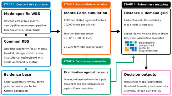
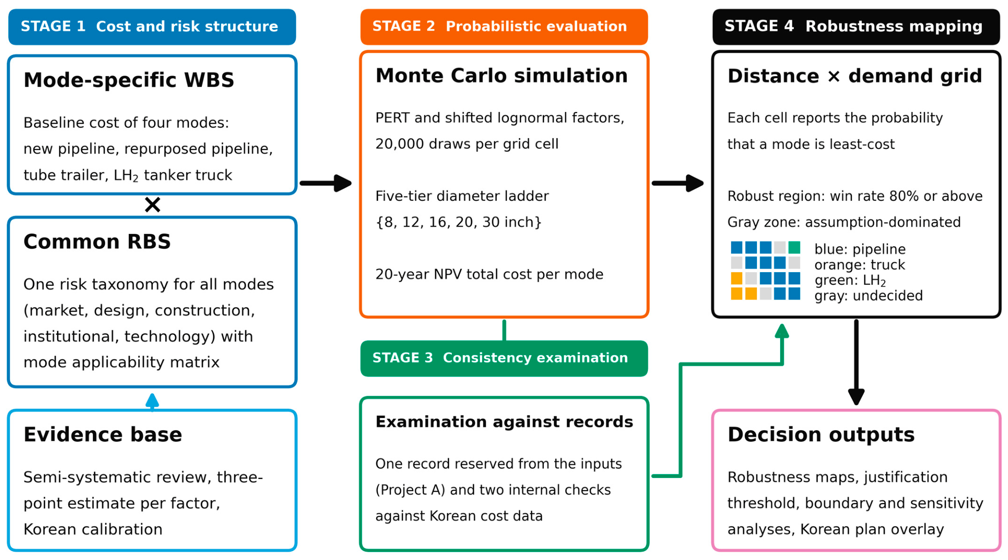
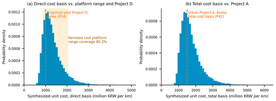
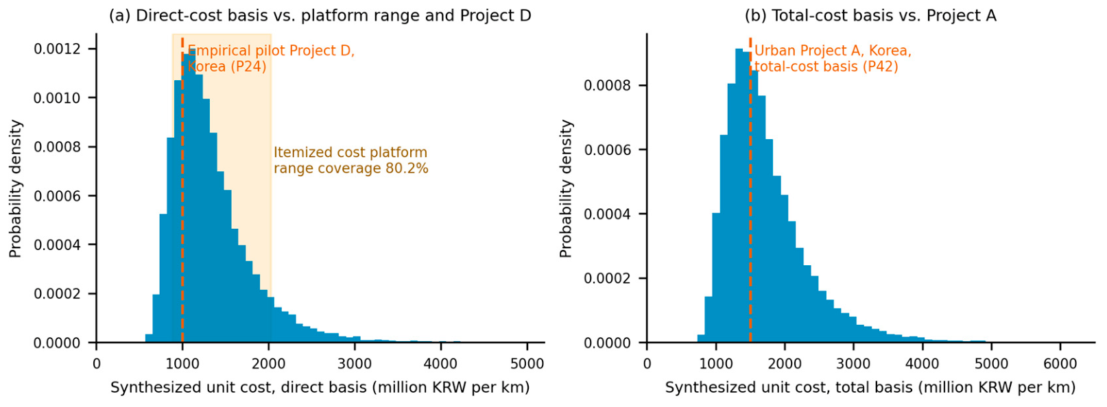
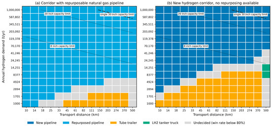
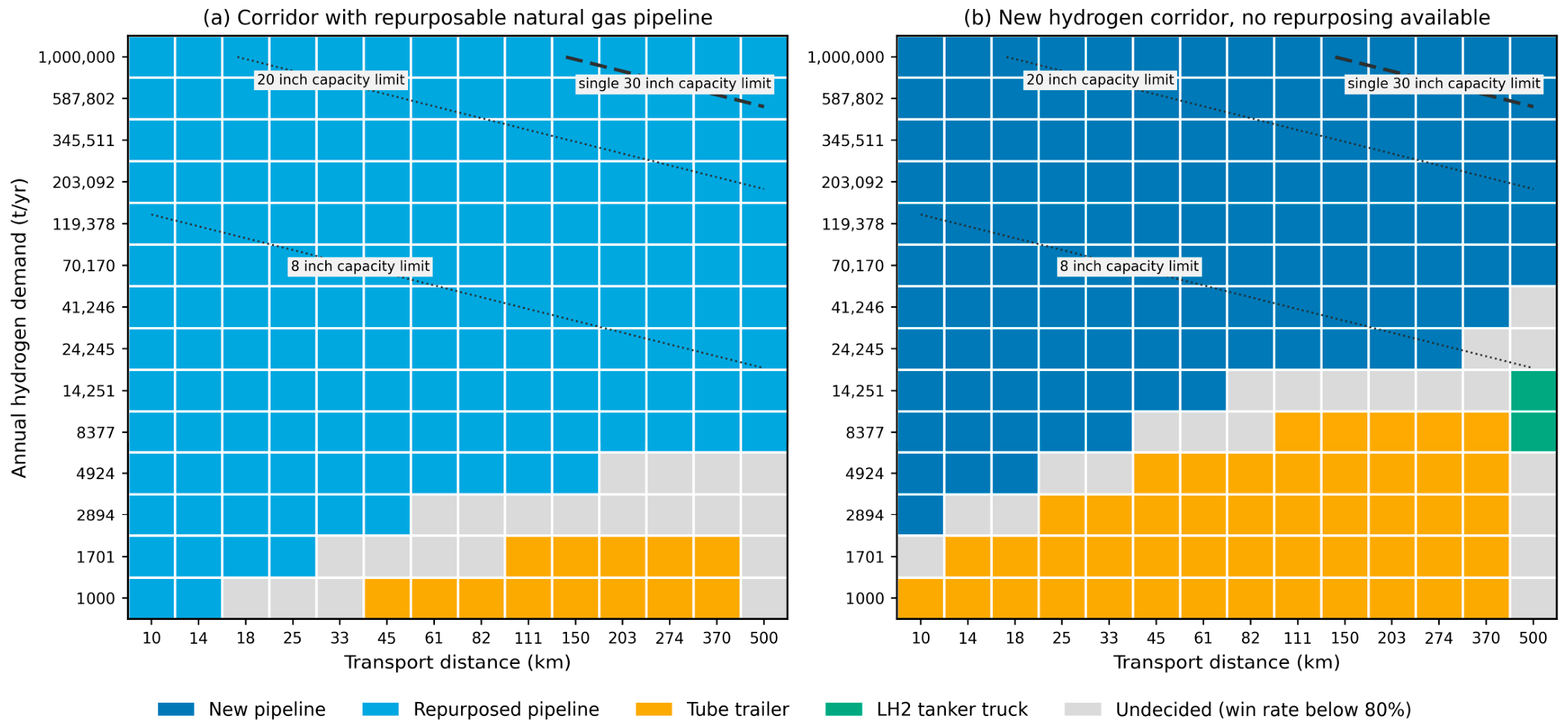
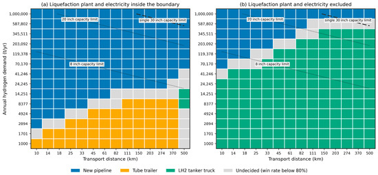
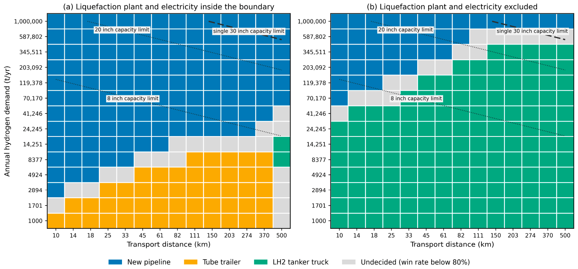
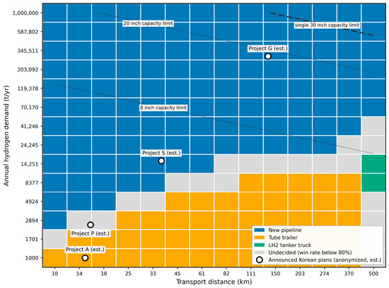
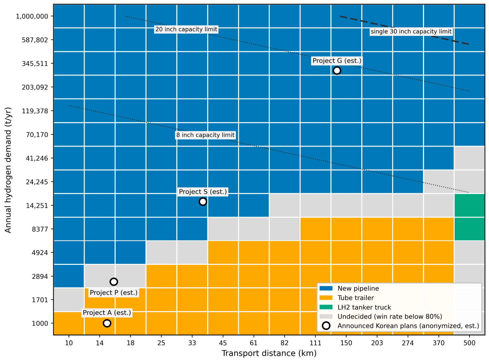
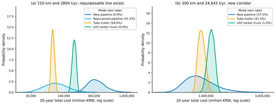
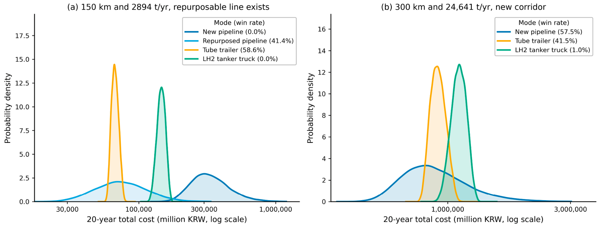
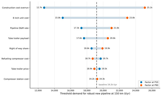
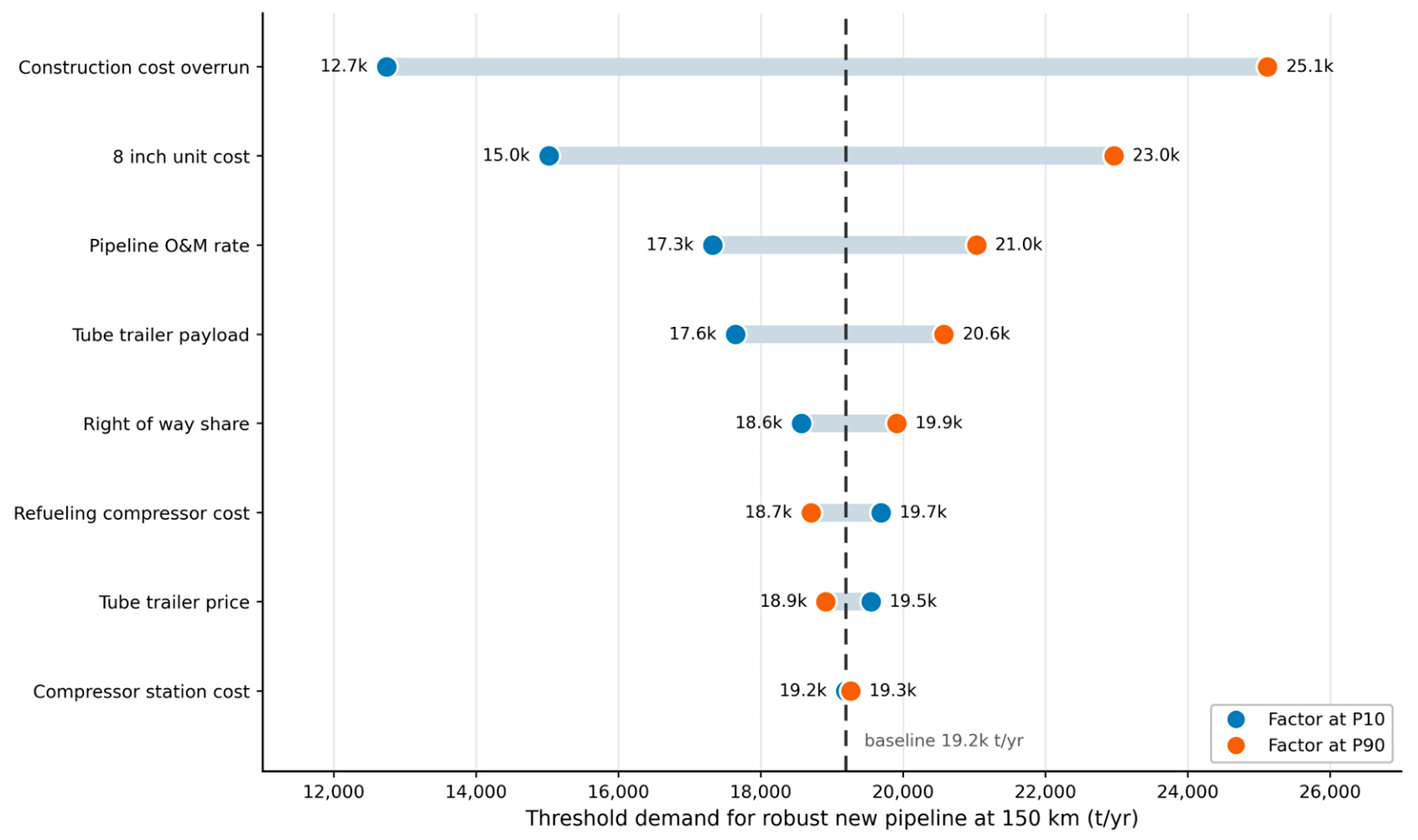
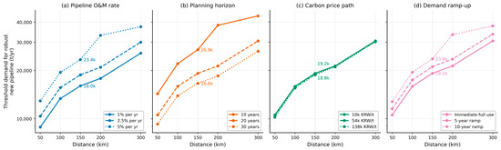
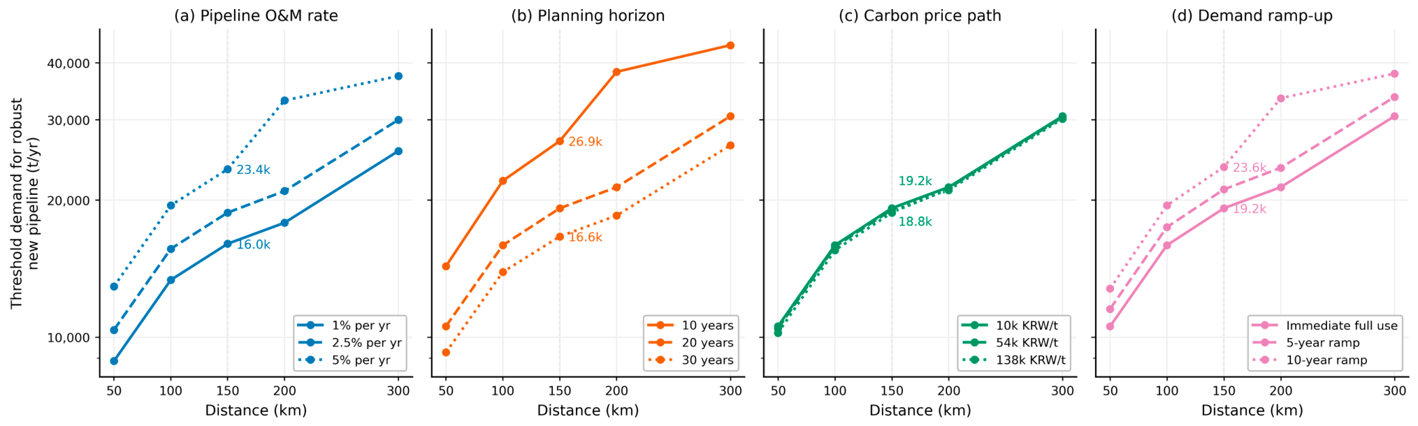

Disclaimer/Publisher’s Note: The statements, opinions and data contained in all publications are solely those of the individual author(s) and contributor(s) and not of MDPI and/or the editor(s). MDPI and/or the editor(s) disclaim responsibility for any injury to people or property resulting from any ideas, methods, instructions or products referred to in the content. |
© 2026 by the authors. Licensee MDPI, Basel, Switzerland. This article is an open access article distributed under the terms and conditions of the Creative Commons Attribution (CC BY) license.