


Abstract
High renewable penetration makes imbalance settlement inseparable from the physical decisions governing reserve procurement and flexibility activation. This paper develops a decision-focused learning-based optimization framework that trains renewable-deviation and flexible-resource deliverability representations through downstream dispatch, reliability, and settlement consequences. The mathematical contribution is a settlement-aware learning objective that couples learned uncertainty, resource-time credible-capacity certification, network-constrained multi-stage dispatch, and counterfactual marginal-contribution allocation while retaining an exact revenue-adequacy identity. The 33-node Zhangjiakou-type regional case uses 15 min intervals and comprises five resource classes: independent storage, data-center flexibility, industrial adjustable load, commercial demand response, and electric-vehicle aggregation. Relative to a fixed-ratio reserve rule, the proposed method lowers the regional balancing cost from 950 to 618 thousand USD (34.9%), achieves 97.8% renewable accommodation, limits the shortage probability to 0.7%, and attains a settlement-fairness index of 0.92. The framework solves a 500-asset instance in 118 s. External validation uses 4027 half-hour observations from the 2025 Elexon/BMRS market, including measured wind and solar output, day-ahead forecasts, load, imbalance prices, and procured-reserve prices. On the 1487-interval December test set, the proposed model reduces the replay cost from 2953.3 to 2598.2 thousand GBP (12.0%), decreases the shortage-interval frequency from 4.64% to 1.28%, and reaches 99.74% renewable accommodation. Comparisons with forecast-then-optimize, Wasserstein distributionally robust optimization, off-policy reinforcement learning, and graph-based behavioral cloning establish that the improvement comes from jointly learning which uncertainty matters for dispatch and which flexible capacity is deliverable.
1. Introduction
The rapid expansion of wind and solar generation has changed the operating logic of modern electricity markets. In conventional systems, imbalance settlement was primarily an ex post financial instrument: a renewable producer, load-serving entity, or market participant deviated from its schedule and paid a deviation charge calculated after physical balancing. Under high renewable penetration, this logic becomes incomplete because the financial settlement is inseparable from the real-time physical decision that prevents reserve shortage, wind spillage, photovoltaic curtailment, and frequency-security degradation. Forecast errors are no longer small residuals around dispatchable thermal production. They are structured, weather-driven, and often correlated across neighboring renewable plants and load zones. This creates a new research problem: imbalance management must be formulated as a coupled learning, optimization, and settlement problem rather than a pure forecasting problem or a pure market-pricing problem.
Wind power forecasting and probabilistic forecast calibration have been studied extensively, and the literature has shown that forecast value depends on the operational decision in which the forecast is used [1]. Reserve-market studies further indicate that the economic value of balancing capacity depends on the joint distribution of renewable uncertainty and system flexibility [2]. However, the practical settlement rules used in many markets still apply deterministic deviation bands, fixed penalty factors, or administrative reserve requirements. These rules are transparent but insufficiently adaptive. They do not distinguish between deviations that actually create reserve scarcity and deviations that are absorbed by already-available flexibility. They also cannot evaluate the deliverable capacity of new flexible resources whose availability depends on state of charge, computational workload, industrial production processes, or customer response fatigue.
The need for an integrated decision model has become more urgent as the power system evolves into a cyber–physical and multi-energy platform. Recent grid-resilience studies after large disturbances emphasize that inverter-rich, automated, and highly coupled systems may exhibit interaction patterns that cannot be captured by isolated reliability margins [3]. Risk-averse dispatch and safe learning methods have begun to integrate frequency-security constraints into learning-based dispatch, demonstrating that artificial intelligence can be embedded into safety-aware operating models rather than used only as an external predictor [4]. Distributionally robust operational risk assessment has also shown that high wind penetration requires uncertainty sets and risk metrics that are computationally fast enough for operational use [5]. These advances motivate a formulation in which learning models are trained for their ability to improve market and dispatch decisions.
Recent work in Energies sharpens this motivation. Off-policy reinforcement learning has been used for economic dispatch with an ensemble reward design [6], graph neural networks combined with behavioral cloning have accelerated topology-aware real-time scheduling [7], open balancing-market simulation has exposed how reserve-market and imbalance-settlement rules interact [8], and coordinated renewable–demand-response trading has shown that flexibility uncertainty directly changes imbalance exposure [9]. Safe-economic and fairness-aware renewable dispatch has also been formulated as a two-stage scheduling problem [10]. These studies establish strong learning, graph, market-simulation, and fairness baselines. However, they do not train the uncertainty representation through a dispatch model that simultaneously certifies deliverable flexible capacity and produces revenue-adequate participant-level imbalance charges.
This paper develops a decision-focused learning-based optimization framework for renewable imbalance settlement and flexible resource dispatch. The term decision-focused is important. In a forecast-then-optimize pipeline, a machine-learning model first minimizes a statistical loss, such as mean absolute error, pinball loss, or negative log-likelihood. The resulting forecast is then passed into a market-clearing or reserve-dispatch optimization model. This two-step process can be suboptimal because the forecast components that most affect downstream imbalance cost may not be the components that dominate the statistical error. For example, a small underforecast during a scarcity period can be more expensive than a large overforecast during a low-load period. Similarly, a forecast error at a node with limited flexible resources can be more consequential than an error at a node with abundant storage. Decision-focused learning directly internalizes this asymmetry by training the prediction model through the optimization loss induced by the dispatch and settlement model.
The proposed framework has three research objectives. First, it learns renewable deviation representations that are operationally meaningful for reserve procurement and real-time balancing. The learned representation describes not only the expected forecast error but also tail-risk scenarios, temporal persistence, nodal correlations, and uncertainty around flexible-resource availability. Second, it certifies the credible capacity of heterogeneous emerging flexible resources and dispatches them through a multi-stage optimization model. The model covers day-ahead reserve procurement, intraday adjustment, real-time activation, reserve shortage, renewable curtailment, and operating constraints of storage, data centers, industrial flexible loads, commercial response, and electric-vehicle aggregators. Third, it designs a responsibility-aware settlement mechanism that allocates imbalance costs between renewable-side and load-side participants according to their learned marginal contributions to system imbalance. The mechanism follows the principle that each participant should bear the marginal balancing cost imposed by its deviation, while preserving settlement budget balance and flexible-resource participation incentives.
From a market-design perspective, this shift is not simply a technical improvement; it changes the definition of accountability. In a traditional deviation-charge system, the settlement rule observes the difference between a submitted schedule and an actual metered quantity, and then applies a price. Such a rule is easy to audit but may be economically inaccurate when the system has multiple sources of flexibility and multiple drivers of reserve activation. A renewable producer may create a deviation that is absorbed by low-cost storage, while another smaller deviation may occur during a congested interval and require expensive load interruption. The two deviations should not necessarily receive the same charge. Similarly, a load-side participant may increase consumption during a scarcity interval and materially worsen the reserve requirement even if its deviation is smaller than that of a renewable plant. Therefore, the settlement design must reflect both physical causality and economic marginal contribution. The proposed formulation operationalizes this idea by making the settlement coefficient a function of counterfactual balancing cost, learned deviation patterns, and resource scarcity.
This paper also addresses a second implementation challenge: emerging flexible resources cannot be treated as firm capacity. A battery with a high power rating may have low credible upward capacity if its state of charge is depleted. A data center may have substantial electrical load but only a portion can be shifted without violating service quality. An industrial user may provide deep reduction during one event but require a recovery period before the next event. An electric-vehicle aggregator may provide fast response only when enough vehicles are connected. These characteristics imply that flexible-resource capacity must be certified dynamically. The proposed model therefore distinguishes between technical maximum capacity, learned credible capacity, certified reserve capacity, and real-time activated capacity. This distinction is essential for a marketized reserve product because it prevents over-procurement from unreliable resources and avoids undercompensation of resources that deliver high-quality response.
The contribution is not the independent invention of decision-focused learning, Wasserstein ambiguity sets, chance constraints, Shapley values, or reserve procurement. Those elements retain their established definitions. The new formulation lies in their mathematical coupling. First, the training loss contains realized dispatch cost, tail reliability, settlement fairness, and revenue-adequacy residuals, so prediction errors receive weights determined by their physical and financial consequences. Second, resource-time deliverability enters the optimization layer through learned credible-capacity bounds; the gradient therefore reflects both renewable uncertainty and the probability that committed flexibility will actually respond. Third, each participant’s settlement share is obtained from a counterfactual redispatch value function with the day-ahead commitment fixed, and the resulting non-negative Shapley weights scale an explicit balancing-revenue requirement. This construction guarantees revenue adequacy by identity rather than checking it after simulation. Fourth, the integrated formulation is evaluated against fixed-ratio, forecast-then-optimize, Wasserstein distributionally robust optimization, off-policy reinforcement learning, and graph-based dispatch baselines on both a network-constrained regional case and an actual-market replay.
Table 1 delineates the established foundations retained in the framework and the mathematical roles developed in this study.
Table 1.
Originality boundary of the proposed formulation.
The remainder of this paper is organized as follows: Section 2 reviews related work on renewable imbalance management, learning-based optimization, and emerging flexible resources. Section 3, Section 4 and Section 5 present the proposed mathematical model. Section 3 defines the decision-focused learning architecture, Section 4 formulates the multi-stage flexible dispatch and capacity-certification problem, and Section 5 develops the responsibility-aware settlement mechanism and solution approach. Section 6 describes the data, experimental design, parameters, and benchmarks. Section 7 reports the numerical results, and Section 8 concludes the paper.
2. Literature Review
2.1. Renewable Imbalance Management, Reserve Procurement, and Market Settlement
Renewable imbalance management has traditionally been studied through forecasting, reserve valuation, and market settlement. Probabilistic wind forecasting provides a foundation for scenario generation, risk-aware scheduling, and quantile-based reserve procurement [11]. Early non-parametric wind-power forecasting work showed that distributional forecasts are more useful than point forecasts when operators must decide reserve margins and imbalance penalties [12]. These ideas support the present study, but the proposed framework departs from the forecasting-centered view by making the forecast representation endogenous to the optimization objective.
The operating-reserve literature emphasizes that the value of reserve depends on scarcity, response speed, and the opportunity cost of resources. Stochastic operational planning with wind generation has shown how uncertainty can be embedded in security-constrained dispatch decisions [13]. Multi-area stochastic unit commitment studies further demonstrate that wind uncertainty creates geographically differentiated reserve needs, especially when transmission constraints limit balancing transfers [14]. Textbook treatments of renewable market integration have formalized the relationship among uncertainty, reserve scheduling, and market-clearing design [15]. Stochastic market designs for wind producers further show that imbalance exposure changes optimal bidding and reserve behavior [16]. These studies are essential, but they normally assume that the uncertainty model is exogenous or pre-estimated. The present paper instead trains the uncertainty representation according to dispatch and settlement consequences.
Recent multi-energy and virtual-power-plant studies provide direct motivation for the flexible-resource dimension of this paper. Temporally coordinated operation of green airport microgrids has demonstrated that flexible loads, climatic correlations, hydrogen storage, and stochastic programming can be integrated in a decomposed operational model [17]. Carbon-oriented collaborative pricing in multi-energy systems further shows that price and operation layers must be coordinated when energy carriers and flexible resources interact [18]. Virtual power plant models for inertia and primary frequency response show that distributed resources can be aggregated into ancillary-service products when their dynamic response characteristics are properly represented [19]. Dynamic construction strategies for virtual power plants extend this logic by recognizing that distributed-resource interactions and response recovery processes determine the feasible aggregation boundary [20]. These works support the flexible-resource pool concept adopted here, while the present paper focuses on imbalance settlement and source–load cost responsibility.
Hydropower, storage, and high-wind operational risk studies also provide relevant modeling insight. Carryover storage valuation in cascaded hydropower planning shows that intertemporal energy value must be internalized when a storage-like resource is used for both current balancing and future operation [21]. This is closely related to battery energy storage in imbalance settlement, because excessive real-time activation may reduce future reserve deliverability. Model-free voltage calculation for active distribution networks shows that data-driven methods can provide operational models when physical topology or parameters are incomplete [22]. Oscillation-source-location studies in power systems show that event attribution is necessary for post-disturbance accountability and control response [23]. The settlement layer in this paper follows the same attribution logic: imbalance costs should be traced to the sources and loads that materially contribute to reserve activation.
2.2. Learning-Based Optimization and Decision-Focused Learning
Learning-based optimization has emerged to overcome the limitations of sequential forecast-then-optimize pipelines. In classical stochastic programming, the uncertainty distribution is specified before optimization, and theoretical foundations for scenario-based decision models are well established [24]. Sample average approximation is then used to construct a tractable deterministic equivalent [25]. Decomposition methods then exploit the structure of large-scale stochastic programs and mixed-integer programs [26]. Although these methods are rigorous, they do not prescribe how a predictive model should be trained when the final goal is economic decision quality rather than statistical forecast accuracy. Decision-focused learning addresses this gap by training the predictor through the optimization objective itself.
Task-based end-to-end learning for stochastic optimization was among the earliest energy-system formulations of this idea and demonstrated that predictions should be judged by their induced operational cost [27]. The melding of data and decision pipelines extended the decision-focused view by showing how machine-learning models can be integrated with combinatorial optimization problems [28]. The smart predict-then-optimize framework provided a structured loss function for training prediction models in downstream linear optimization settings [29]. Differentiable optimization layers, such as OptNet, enabled constrained optimization problems to be embedded within neural networks [30]. Differentiable convex optimization layers later made this approach more general and practical for disciplined convex programs [31]. These methodological foundations are directly relevant to the present model, where renewable-deviation representations are trained according to the cost of dispatch and settlement decisions.
Robust and distributionally robust optimization are also central to learning-based decision models under renewable uncertainty. The price-of-robustness framework formalized how uncertainty protection can be selected without making operations excessively conservative [32]. General robust optimization theory provides the broader mathematical basis for converting uncertain constraints into tractable deterministic equivalents [33]. Moment-based distributionally robust optimization introduced ambiguity sets that preserve tractability when only partial distributional information is known [34]. Wasserstein distributionally robust optimization allows ambiguity sets to be learned from empirical samples, making it attractive for renewable-forecast deviations and flexible-resource availability [35]. Conditional value-at-risk provides a coherent way to penalize tail-cost outcomes caused by reserve shortage, curtailment, or expensive emergency activation [36]. The proposed framework combines these ideas with decision-focused learning so that the ambiguity representation, risk penalty, and reserve decisions are co-designed.
2.3. Emerging Flexible Resources and Source–Load Responsibility Allocation
Demand-side and distributed flexible resources have become central to renewable-dominated power systems. Early demand-side market analysis emphasized that electricity demand is not purely passive and that load flexibility can alter market efficiency and reliability [37]. Demand-response and smart-load surveys then classified the operational mechanisms through which customers can provide load reduction, shifting, and ancillary services [38]. The virtual power plant concept proposed a market-oriented aggregation structure for distributed generators, storage devices, and controllable loads [39]. Mid-term dispatch optimization of virtual power plants showed how aggregation can be scheduled under market and technical constraints [40]. Bidding studies for virtual power plants in energy and reserve markets further clarified that aggregated flexibility must be priced and settled according to both energy and reserve value [41]. These ideas are integrated in the reserve-pool and market-clearing layers of the proposed model. The scope of emerging flexibility is now broader than traditional demand response. Energy storage can shift renewable energy across hours and provide rapid balancing, but its opportunity cost depends on intertemporal state of charge and future scarcity. Storage valuation studies in electricity markets provide evidence that arbitrage value, reserve value, and congestion value must be jointly considered [42]. Renewable integration studies further emphasize the role of storage in reducing curtailment and improving system flexibility [43]. Data centers can provide flexible load by temporal workload shifting, cooling adjustment, or geographic load migration; classic Internet-scale system studies show that electricity cost can be reduced when computational workloads respond to energy prices [44]. Electric vehicles can act as distributed storage, and vehicle-to-grid research has long recognized their potential to provide regulation and renewable balancing services [45]. In the present paper, these resource classes are represented in a unified dispatch and certification model.
Multi-energy coupling and sector integration also influence flexible-resource dispatch. The role of hydrogen in future sustainable transport and energy systems illustrates how power, transport, storage, and industrial sectors increasingly form one flexibility ecosystem [46]. Data-model hybrid scheduling for grid-connected PEM green hydrogen production shows that multi-energy flexibility requires coordination between physical process models and data-driven scheduling decisions [47]. These works motivate the inclusion of state-dependent, energy-limited, and service-quality-constrained flexibility in renewable imbalance settlement. The key gap addressed in this paper is that existing resource models rarely connect flexible-resource dispatch with responsibility-aware imbalance settlement. A market can procure and dispatch flexible resources efficiently, but if the settlement rule fails to trace who caused the reserve activation, incentives remain distorted. The proposed model therefore combines dispatch optimization with source–load marginal contribution tracing.
The literature therefore leaves three linked gaps. First, probabilistic forecasting studies often evaluate calibration and sharpness without measuring whether the resulting distribution improves imbalance settlement. Second, stochastic and robust dispatch studies optimize operating decisions but usually assume that the uncertainty model has already been selected. Third, market-mechanism studies examine reserve pricing, virtual power plant participation, or demand response incentives, but they rarely embed responsibility allocation directly into the physical dispatch optimization. The present paper closes these gaps by co-designing the learned uncertainty representation, the reserve-dispatch optimization, and the settlement-cost allocation rule. This co-design is particularly relevant for regional pilots, where the operator must justify not only the total balancing cost but also the distribution of charges among renewable generators, load-side users, aggregators, and flexible-resource providers.
Figure 1 distinguishes the forward computation from the training feedback. Renewable forecasts, realized generation, load, resource states, and market records enter the learning layer, which produces deviation scenarios and resource-time deliverability probabilities. The probabilities impose credible-capacity limits, and both outputs enter the same network-constrained dispatch. Real-time activation then determines the counterfactual redispatch value used for settlement. Cost, shortage, curtailment, fairness, and revenue adequacy are evaluated after settlement, and the resulting weighted decision loss is differentiated back to the learning model. No arrow bypasses physical feasibility or settlement accounting.
Figure 1.
Schematic of the decision-focused learning-based optimization framework. Solid arrows trace the forward market-clearing and settlement sequence; the separated dashed blue path returns the composite decision-loss gradient to the learning layer.
3. Decision-Focused Learning Architecture
This section defines the learning-to-decision architecture that connects renewable-deviation data, flexible-resource availability, optimization decisions, and imbalance settlement. Let denote the set of dispatch intervals, the set of renewable generators, the set of flexible resources, the set of network nodes, and the set of scenarios. Historical data include renewable forecasts, actual generation, meteorological variables, nodal loads, resource states, market-clearing results, and settlement outcomes. The training sample is defined as
where contains weather and calendar features, and are forecast and actual renewable outputs, is load, is the state of flexible resources, and collects market and settlement labels. Renewable deviation is measured by
The learning model maps observable features to a conditional distribution of uncertainty,
where denotes trainable parameters and includes renewable deviations, load deviations, and flexible-resource availability shocks.
A scenario generator converts the learned distribution into optimization scenarios:
where is an exogenous random seed or a latent uncertainty sample. Given , the downstream optimization returns the optimal decision vector,
where contains reserve procurement, certified capacity, flexible-resource activation, curtailment, shortage, and settlement variables. The decision-focused objective extends the established predict-then-optimize loss by including the reliability and settlement consequences generated downstream:
where is the non-negative revenue-adequacy residual defined in Section 5. The coefficients selected on the validation set are , , , and . The gradient of the composite decision loss is
When the downstream problem is convex after fixing integer commitment variables, implicit differentiation through optimality conditions can be used:
Here, is the Lagrangian, are dual multipliers, and represents inequality constraints.
Calibration is maintained through a distributional scoring loss,
where is the pinball loss and is the learned quantile. To provide reliability protection, an empirical Wasserstein ambiguity set is constructed as
where is the Wasserstein distance and is a learned or validated radius. Reserve shortage risk is summarized by
where is renewable underproduction, is load overconsumption, and is upward reserve.
For each flexible resource r, the learning model estimates a deliverability probability:
where includes state of charge, workload, industrial operating mode, customer response history, or electric-vehicle plug-in probability. Credible capacity is then certified as
where is a performance derating coefficient and is the technical maximum capacity. The learned activation cost is represented by
where the coefficients are learned from bids, historical activation, degradation cost, and response-recovery records.
The marginal contribution feature of participant i to imbalance is defined as
where denotes a counterfactual system in which participant i’s deviation is removed. A source–load responsibility vector is learned as
where contains contractual schedules, historical compliance scores, and nodal scarcity indicators. Online learning updates the parameter vector according to
where is an adaptive step size. The integrated learning target is finally written as
The predictor used in every reported experiment is a two-hidden-layer quantile network with 64 and 32 rectified linear units. Inputs comprise 24 lagged renewable deviations, eight lagged load deviations, sine and cosine time encodings, weekday, forecast renewable output, forecast load, and the most recent resource states. The model outputs the 0.05, 0.25, 0.50, 0.75, and 0.95 conditional quantiles and the five resource-class deliverability probabilities. Training used Adam, a batch size of 256, an initial learning rate of , 100 epochs, early stopping after 12 validation epochs, and random seed 4446492. Each training dispatch used 64 reparameterized scenarios; final evaluation used 200 scenarios. All continuous decisions were differentiated through the KKT system in Equation (8); binary day-ahead commitment variables were fixed at their incumbent values within a gradient batch and re-optimized between batches.
The Wasserstein radius in Equation (10) is dimensionless because every uncertainty coordinate is standardized by its training-set standard deviation. The candidate set was evaluated chronologically on the validation period. The selected value, , minimized the validation balancing cost subject to shortage probability no greater than 1%. The chance-constraint form and Wasserstein ball are therefore inherited tools; their joint dependence on the decision-trained deviation distribution and learned deliverability bounds is specific to the proposed layer.
The practical interpretation of this architecture is as follows: The learning component observes historical dependencies among weather conditions, forecast errors, load deviations, and resource responses. It does not merely predict a single net imbalance value. Instead, it learns a structured representation that the optimization model can query to determine the upward reserve requirement, the location of probable reserve shortages, the flexible resources likely to be deliverable, and the participants likely to generate costly deviations. The optimization component then converts this representation into market decisions. If the learned model overstates a deviation that is inexpensive and nonbinding, the downstream loss imposes only a weak penalty. If it understates a deviation that creates scarcity, the optimization loss rises because the system incurs reserve-shortage or emergency-activation costs. This asymmetric weighting is the principal mechanism of decision-focused training.
Another important feature is interpretability. Decision-focused learning is sometimes criticized because end-to-end training may reduce transparency. In this paper, interpretability is preserved by explicitly separating the learned components from the market-clearing structure. The model learns deviation distributions, credible capacity coefficients, activation-cost parameters, and responsibility features. The reserve-balance, storage-state, service-quality, network, and settlement-budget relationships remain explicit. As a result, market operators can audit why a reserve requirement increased, why a resource received a lower certified capacity, or why a participant received a higher imbalance charge. This structure is compatible with regulatory review because the learning model supports decisions but does not replace the market-clearing logic.
The learning layer is not an external forecasting module. It is a market-facing representation engine whose parameters are trained by the cost and reliability consequences of the downstream optimization.
4. Multi-Stage Optimization for Flexible Resource Dispatch
This section formulates the multi-stage reserve procurement, capacity certification, and real-time dispatch model. The system operator minimizes the expected total cost of reserve procurement, flexible-resource activation, renewable curtailment, reserve shortage, and settlement imbalance:
The upward reserve requirement is linked to the learned deviation quantile:
The certified capacity of all flexible resources must cover the procured reserve volume:
Each certified capacity is bounded by the credible capacity learned in Section 3:
The capacity procurement cost is
where is the capacity offer price or market-clearing price. Real-time balance under each scenario is enforced by
Renewable generation is determined by forecast output, learned deviation, and curtailment:
Battery storage energy evolves as
The storage state and power outputs satisfy
Data-center load reduction is bounded by workload elasticity:
The service-quality constraint for data centers is
Industrial load response is bounded by process limits:
The rebound process after industrial or commercial load reduction is modeled as
Rebound power must be incorporated into load balance:
Electric-vehicle aggregator energy satisfies
EV mobility requirements are enforced by
Flexible-resource activation cannot exceed certified capacity:
Ramping limits are
Nodal power balance under a DC network approximation is
Transmission security is enforced by
Reserve shortage is non-negative and penalized heavily:
Renewable curtailment is bounded by available renewable generation:
The chance constraint for reserve sufficiency is
A distributionally robust counterpart is represented by
Table 2 states the exact calculation sequence. In the objective, , , and . Upward reserve is therefore not calculated as an unexplained residual: the validated uncertainty quantile sets the system requirement, learned deliverability bounds each offer, the master problem selects the certified capacity, and each scenario subproblem resolves resource activation subject to Equations (24)–(42).
Table 2.
Implemented calculation sequence for flexible-resource dispatch.
The reported regional experiments used the scenario-based deterministic equivalent with a Benders master problem for certified capacity and one second-stage quadratic dispatch subproblem per scenario. The implementation used Python 3.11, PyTorch 2.3.1, CVXPY 1.5.3, and Gurobi 11.0.3. Gurobi used an optimality gap of , a feasibility tolerance of , eight solver threads, and a 600 s limit; no reported instance reached that limit. Benders iterations stopped when the relative upper–lower bound gap fell below . The computing platform comprised an Intel Xeon Gold 6338 CPU, 256 GB RAM, and an NVIDIA RTX A5000 GPU. These settings underpin the computational results reported in Section 7.
5. Responsibility-Aware Imbalance Settlement and Solution Approach
The settlement model converts the complete physical balancing requirement into auditable charges and payments. Capacity procurement is included because it is incurred to cover the realized uncertainty even when part of the reserve remains unactivated. For each scenario,
The normalized settlement weight uses the sampled Shapley contribution defined in Equation (47). The equal-weight branch is invoked only when every contribution is non-positive:
The counterfactual marginal contribution of renewable generator g is
The counterfactual marginal contribution of load participant n is
For coalition-based settlement, an approximate Shapley value is calculated as
The source-side charge is
The load-side charge is
Flexible resources receive capacity and activation payments:
Because the weights in Equation (44) sum exactly to one, revenue adequacy is an identity rather than an empirical check:
Participation compatibility for flexible resource r is
Settlement fairness is measured by the deviation between assigned cost and marginal contribution:
A Benders-type master problem optimizes first-stage reserve capacity:
The online solution stops when the primal-dual residual is below tolerance:
The settlement layer is designed to avoid three distortions common in imbalance-pricing practice: The first distortion is socialization without causality, in which all users share balancing costs even if only a subset of participants caused the reserve activation. The second distortion is mechanical deviation pricing, in which charges are proportional to energy deviation but ignore whether the deviation occurred during scarcity, congestion, or surplus. The third distortion is undercompensation of flexible resources, in which availability is undervalued and resources have little incentive to maintain deliverability. The proposed settlement mechanism mitigates these distortions by linking participant charges to counterfactual marginal cost and linking flexible-resource payments to both certified capacity and real-time activation.
The coalition value in Equation (47) is implemented as . Members of retain their realized deviations; participants outside are set to their contracted schedules. The day-ahead certified capacities and network topology are held fixed, while storage, flexible-load activation, curtailment, line flows, and shortage are re-optimized in every scenario. This construction isolates the cost caused by the coalition without crediting it for a different first-stage procurement decision. Source-side and load-side participants may enter the same coalition; their signs are retained, so a load deviation that offsets renewable underproduction can reduce the coalition value.
Exact enumeration requires redispatches. The reported settlement uses 500 antithetic random permutations, evaluates every participant’s entry along each permutation, and averages the marginal increments. The same scenario draws are used for adjacent coalitions to reduce Monte Carlo noise. Independent permutation batches are run until the maximum change in any participant share is below 1%; the 500-permutation cap is binding only for the 250- and 500-participant cases. Redispatches are parallelized across 32 CPU workers. Table 3 reports the resulting cost and allocation error against a 2000-permutation reference.
Table 3.
Computational cost of sampled Shapley settlement.
Equation (51) guarantees revenue adequacy for every interval and every participant set because the non-negative weights sum to one and are applied to the complete balancing-revenue requirement. The result is not limited to the numerical examples. The equal-weight branch prevents an undefined denominator in the exceptional case where no positive contribution exists. Numerical rounding is performed only after aggregation to currency units; the unrounded settlement residual remained below GBP in all experiments.
6. Data, Experimental Design, and Parameters
The empirical design has two distinct evidence layers. The first is a network-constrained regional engineering case used to test the complete learning, reserve, dispatch, and participant-level settlement mechanism. It contains 33 nodes, 32 branches, four conventional units, ten wind plants, six photovoltaic plants, and 200 flexible-resource aggregations in the baseline configuration. The chronology contains 35,040 15 min intervals. Public market trajectories are regionalized by per-unit scaling, while the network, flexible-resource ratings, and response constraints are fixed engineering inputs; day-ahead, intraday, and real-time market outputs are generated endogenously by the optimization model. The second layer is an external replay of the actual Great Britain balancing market. It uses Elexon/BMRS day-ahead wind and solar forecasts (DGWS/B1440), measured or estimated wind and solar output (AGWS/B1630), actual total load (ATL/B0610), system imbalance prices (DISEBSP), and procured upward-reserve prices (PPBR/B1730) [48]. This replay tests the learned reserve policy against recorded market-level uncertainty and prices rather than simulated market-clearing outputs. Keeping the two layers separate prevents the historical replay from being used to support participant-level or nodal claims: the regional case evaluates mechanism completeness, whereas the replay evaluates reserve-policy transfer under recorded market conditions. Table 4 summarizes the sources, resolutions, system sizes, and chronological splits for both evidence layers.
Table 4.
Datasets, temporal resolution, system size, and chronological splits.
Figure 2 contains 2050 MW of nameplate flexibility, 1585 MW of mean available capacity, and 1271 MW of P10 deliverable capacity. Independent storage retains 352 of 480 MW at P10 (73.3%), whereas industrial adjustable load retains 360 of 620 MW (58.1%). The corresponding P10 ratios are 63.9% for data centers, 55.7% for commercial demand response, and 56.9% for EV aggregation. Thus, treating nameplate power as firm reserve would overstate dependable capacity by 779 MW, or 38.0% of the technical total. Table 5 supplies every bar value used in the figure.
Figure 2.
Flexible-resource capacity inputs for the 33-node regional case. Technical maximum is the nameplate response limit; the historical mean and P10 values are calculated from the resource-state and response records used for credible-capacity calibration.
Table 5.
Numerical capacity values underlying Figure 2.
In Figure 3, aggregate load ranges from 480 to 602 MW, wind from 107 to 260 MW, solar from 0 to 247 MW, and net load from 100 to 386 MW. The highlighted scarcity window from Thursday 17:00 to Friday 03:00 combines a 386 MW net-load peak with declining solar output. These values are regionalized test-system inputs rather than market-clearing outputs. The caption identifies their source, resolution, aggregation level, and system size, specifying the operating conditions independently of the optimization results.
Figure 3.
Seven-day operating excerpt from the 33-node regional case. The 15 min input is aggregated to 1 h for display; wind, solar, load, and net load are system-wide sums across the ten wind plants, six photovoltaic plants, and 33 load nodes.
Figure 4 reports normalized renewable forecast-error intensity by target hour and forecast lead.
Figure 4.
Normalized renewable forecast-error intensity by target hour and forecast lead. Forecast–actual pairs are derived from Elexon/BMRS B1440 and B1630 records and evaluated after regionalization to the 1000 MW renewable reference.
For hour h and lead ℓ, the heatmap reports with MW. The plotted leads are 1, 3, 6, 12, 24, and 36 h. nMAE rises from approximately 2–5% at short leads to 6.9–9.4% in the 17:00–21:00 band at 36 h. The maximum, 9.4%, occurs at 18:00. This calculation uses forecast–actual pairs only; no optimized dispatch or simulated price enters the heatmap. The result explains why a uniform statistical loss underweights a limited number of evening cells that create disproportionate reserve and settlement cost.
Figure 5 shows the pre-optimization deliverability landscape for heterogeneous flexible resources. Storage remains highly deliverable over much of the day but is constrained by state-of-charge dynamics, whereas data-center flexibility is more stable because workload shifting and cooling adjustment can provide moderate responses over longer periods. Industrial load has higher availability during operating hours but lower flexibility during production-sensitive intervals. Commercial demand response is most useful in afternoon and early-evening periods, and EV aggregation depends strongly on mobility and charging patterns. The matrix makes clear that a single average availability coefficient would lose important temporal information. The proposed model therefore certifies capacity at the resource-time level, allowing dispatch to select different resources depending on hour-specific deliverability, recovery constraints, and scarcity conditions.
Figure 5.
Hourly deliverability probabilities used for credible-capacity certification in the regional case. Values are estimated from resource states and response-success records before optimization.
Table 6 summarizes the main notation used in the model. The notation is intentionally organized around market decisions rather than physical devices alone, because the objective is to connect technical reserve needs with market settlement. Table 7 describes the data fields and their role in the learning-based optimization pipeline. Renewable forecasts and actual generation construct deviation samples, meteorological features support probabilistic deviation learning, nodal load data identify source–load imbalance interactions, flexible-resource state data determine credible capacity, and market-clearing outputs provide labels for the decision-focused loss. Regional resilience and sector-coupling studies suggest that such multi-source data integration is necessary when power systems interact with hydrogen, transport, industrial production, and automated control layers [46].
Table 6.
Main notation of the decision-focused learning-based optimization model.
Table 7.
Data fields used in the reported experiments.
Table 8 reports the fixed baseline values. Sensitivity experiments vary one quantity at a time around this baseline while retaining all other values.
Table 8.
Implemented baseline parameters for the regional case and actual-market replay.
Every benchmark receives identical chronological splits, scenarios, network limits, resource availability, price inputs, and feasibility restoration. Table 9 supplies the formulation and numerical settings required to reproduce each comparison. Reinforcement learning and graph-based dispatch are included because they represent current data-driven alternatives to repeated mathematical optimization [6,7].
Table 9.
Reproducible benchmark formulations and settings.
Both experiments use chronological rather than random splits. The regional case trains on January–August, validates all hyperparameters on September–October, and reports November–December only once. The external replay trains on 9 October–15 November, validates on 16–30 November, and tests on December 2025. Missing or duplicate records are resolved before splitting; no later observation is used to impute an earlier period. Negative system prices and the highest 1% of imbalance prices remain in the data.
The regional sensitivity grid covers reliability levels , Wasserstein radii , flexible-resource participation from 0 to 100% in 10-percentage-point increments, reserve margins from 0 to 30% in 2-percentage-point increments, and renewable penetration from 30 to 80%. The replay DRO multiplier is selected separately from . Every baseline is fixed before test evaluation. Weekly block bootstrap with 1000 resamples provides the 95% intervals reported for renewable accommodation and actual-market cost.
For the external replay, the reserve head is represented by an auditable 288-state table: six four-hour blocks, renewable-forecast quartiles, one-day-lagged price quartiles, and lagged-error-volatility tertiles. In each state, the proposed policy selects one of 66 actions from 0 to 650 MW, in 10 MW increments, by minimizing price-weighted balancing cost subject to a 0.5% in-state shortage-frequency limit; states with fewer than 25 training observations use the global 0.99 need quantile. This replay-specific compression retains the decision-focused objective while isolating reserve-policy transfer from the full regional nodal and settlement model.
Four ablations were executed with all other settings unchanged: removal of the decision-focused loss, removal of credible-capacity certification, removal of responsibility-aware settlement, and the complete forecast-then-optimize pipeline. A separate rebound ablation confirmed that omitting the recovery load understates the commercial and industrial activation cost by 6.4%; because it changes a device constraint rather than a principal contribution, that result is reported only in the supplementary output.
The reproducible workflow aligns source timestamps, constructs deviations, estimates resource deliverability, trains the quantile and deliverability heads, solves day-ahead and scenario redispatch, and then performs sampled counterfactual settlement. The accompanying script downloads Elexon records without an API key, applies the stated chronological split, reproduces every row of the actual-market table, and exports interval-level reserve, cost, and shortage values.
7. Numerical Results and Discussion
Results are reported in the order of learning validation, reserve clearing, cost decomposition, reliability, capacity certification, settlement, dispatch behavior, sensitivity analysis, computational tractability, and ablation evidence. Regional results use only the November–December test period, and the external replay uses only the December 2025 test period. Unless otherwise stated, costs are totals over the corresponding test set, and probabilities are empirical interval frequencies.
Figure 6 validates the central claim that the proposed learning module is trained for downstream decisions rather than for forecast accuracy alone. The decision-focused training loss declines sharply during the initial epochs and continues to fall, while the validation balancing cost also decreases steadily. The forecast-then-optimize benchmark improves more slowly and remains substantially above the decision-focused validation cost at convergence. The reported 29.2% lower validation cost shows that the model learns the forecast-error features that are most consequential for balancing decisions, not merely the features that reduce average statistical error. Calibration loss decreases at a more moderate rate, which is expected because calibration is retained as a reliability-preserving auxiliary objective. The figure demonstrates that decision-focused learning changes the economic value of the forecast representation.
Figure 6.
Convergence of decision-focused learning and its validation decision-cost advantage over forecast-then-optimize training.
Figure 7 compares reserve procurement, certified flexible capacity, unused reserve, and shortage outcomes across the four clearing methods shown in the figure. The deterministic reserve rule procures a large amount of reserve because it does not adapt to learned uncertainty or resource deliverability. Forecast-then-optimize improves this outcome, but its separate forecast and dispatch stages retain avoidable unused capacity. Wasserstein DRO protects reliability at the cost of additional procurement. The decision-focused model maintains sufficient certified capacity while reducing unused reserve. Table 10 extends the same test to the two recent data-driven comparators and reports all principal regional metrics.
Figure 7.
Reserve procurement and certified flexible capacity under competing market-clearing methods.
Table 10.
Regional test-set comparison at the 60% renewable-penetration baseline. Cost is the total November–December balancing cost; solution time is the mean rolling-horizon clearing time for 200 flexible assets.
The proposed model lowers the regional balancing cost by 34.9% relative to the fixed-ratio rule and by 6.2% relative to Graph-BC, the lowest-cost advanced comparator. Off-policy RL and Graph-BC clear faster because their trained policies replace scenario optimization at inference, but both require feasibility projection and neither jointly optimizes settlement fairness. The proposed method has the lowest shortage probability and the highest renewable accommodation and fairness index while remaining below the 15 min dispatch interval.
Figure 8 decomposes the total regional balancing cost into capacity procurement, activation, curtailment, shortage, and settlement uplift. Table 11 gives the numerical values behind the bars. The deterministic rule produces the highest procurement and shortage expenditures. Wasserstein DRO reduces shortage cost but retains conservative capacity procurement. The proposed method reduces total cost from 950 to 618 thousand USD; 77.4% of the 332-thousand-USD saving comes from capacity, curtailment, and shortage components. Its shortage cost remains positive, confirming that the saving is not created by suppressing the value of lost load or omitting feasibility restoration.
Figure 8.
Regional balancing-cost decomposition obtained from the network-constrained simulation at 15 min resolution. Each component is computed from the cleared quantities and the fixed prices in Table 8; the bars are simulated market outcomes rather than measured Elexon costs.
Table 11.
Numerical values underlying Figure 8 (thousand USD).
Figure 9 evaluates accommodation as renewable penetration rises from 30% to 80%. Table 12 reports the plotted means and uncertainty intervals. Accommodation declines for all methods as penetration rises, but the proposed method remains above 95% at 80% penetration. At that endpoint, it exceeds fixed-ratio reserve by 9.9 percentage points and Wasserstein DRO by 2.7 percentage points. The non-overlapping pointwise intervals between the proposed and fixed-ratio methods at 50–80% penetration show that this ordering is not driven by a single test week.
Figure 9.
Regional renewable accommodation under increasing renewable penetration. Lines show test-set means; shaded bands are 95% weekly block-bootstrap intervals from 1000 resamples.
Table 12.
Numerical values underlying Figure 9: mean renewable accommodation in percent, with the 95% block-bootstrap half-width after “±”.
Figure 10 maps shortage probability over the complete participation and reserve-margin grid. To remain at or below the 1% threshold, the required reserve margin is approximately 20% with no flexible-resource participation, 12% at 50% participation, and 4% at full participation. The bottom-left region violates the threshold because both sources of corrective capacity are scarce. These coordinates make the substitution relationship operational: a 50-percentage-point increase from zero participation lowers the required reserve margin by about eight percentage points in this case.
Figure 10.
Regional reserve-shortage probability across flexible-resource participation (0–100%) and reserve margin (0–30%). The contour denotes the fixed 1% reliability threshold used in the baseline.
Figure 11 evaluates the accuracy and conservatism of the credible-capacity certification procedure. For every resource class, technical maximum capacity exceeds certified credible capacity, confirming that the model does not treat nominal flexibility as firm reserve. Realized delivered capacity is close to certified capacity, indicating that certification is not excessively conservative. Storage has the highest activation success rate, while commercial demand response has the lowest because customer response and recovery behavior are more uncertain. Industrial load has the largest technical potential but a more moderate certified share because process constraints limit dependable activation. The result is operationally important: over-certification would create reserve shortage, while under-certification would waste usable flexibility. The proposed certification model achieves a practical middle ground by aligning reserve offers with historical deliverability and activation success.
Figure 11.
Technical, certified, and delivered flexible capacity by resource class.
Figure 12 shows how responsibility-aware settlement changes the distribution of imbalance costs. The deterministic rule produces the highest total allocated cost and the largest socialized uplift, indicating that a substantial portion of balancing cost cannot be attributed accurately under a fixed rule. Forecast-then-optimize and robust optimization reduce total cost but still retain nontrivial uplift because their settlement layers are not fully coupled with learned marginal contribution tracing. The decision-focused optimization reduces the total allocated imbalance cost to 72 thousand USD and lowers socialized uplift to 5 thousand USD. Renewable generators still bear the largest share because renewable underproduction is a primary driver of upward reserve needs, but load-side participants also receive cost responsibility when their deviations worsen scarcity. This outcome is consistent with the principle that costly imbalance should be allocated to its marginal drivers.
Figure 12.
Responsibility-aware allocation of imbalance costs across renewable generators, load-side resources, and socialized uplift.
Figure 13 reports the optimized hourly activation of flexible resources under the proposed model. Storage is activated most strongly during morning and evening ramp intervals because it provides fast upward reserve and can respond to short-duration scarcity. Data-center flexibility supplies a more stable background contribution, reflecting its ability to adjust computational and cooling loads without major service interruptions. Industrial load activation is concentrated during business hours when process flexibility is available and economically efficient. Commercial demand response becomes more important during afternoon and early-evening conditions, while EV aggregation peaks during the evening ramp when plug-in availability increases. The allocation is physically intuitive and economically meaningful: fast and energy-limited resources are reserved for ramping periods, while slower or more constrained resources are used when their operational limits permit. This confirms that the dispatch layer uses resource heterogeneity rather than aggregating all flexibility into a single reserve block.
Figure 13.
Hourly activation pattern of flexible-resource dispatch under the proposed decision-focused optimization model.
Figure 14 presents a three-dimensional sensitivity surface for balancing cost under different forecast-error severity and reserve-margin settings. The surface exhibits a well-defined cost-efficient region rather than a monotonic relationship. Very low reserve margins expose the system to shortage and emergency activation costs, while excessively high margins increase procurement and opportunity costs. Forecast-error severity shifts the surface upward because larger deviations require more reserve and increase the probability of expensive activation. The valley region indicates the point at which the reserve margin is sufficient to protect reliability without creating excessive unused capacity. This result is valuable for market design because it converts abstract uncertainty into an operational reserve-sizing rule. It also explains why the proposed decision-focused model performs better than fixed rules: it learns where the cost valley lies under changing forecast-error conditions.
Figure 14.
Balancing-cost surface under forecast-error severity and reserve-margin variation.
Figure 15 shows how renewable accommodation depends jointly on flexible-resource participation and renewable penetration. At low flexible participation, accommodation remains limited because the system cannot absorb large renewable deviations without curtailment or shortage. As flexible-resource participation rises, the accommodation surface increases and approaches a high-performance plateau. The surface also shows that very high renewable penetration creates additional stress, but sufficient flexible capacity substantially mitigates this stress. The high-accommodation region is therefore not achieved by renewable expansion alone; it requires coordinated storage, demand response, data center flexibility, industrial load adjustment, and EV aggregation. This figure provides an intuitive system-level explanation for the market mechanism: flexible resources raise the feasible renewable share by expanding the set of balancing actions available to the operator.
Figure 15.
Renewable accommodation surface under flexible-resource participation and renewable penetration.
Figure 16 evaluates computational tractability as the number of flexible assets increases. Deterministic rules solve fastest because they ignore most uncertainty and resource heterogeneity, but their operational quality is inferior. Forecast-then-optimize remains computationally efficient, yet it does not train predictions according to downstream cost. Distributionally robust optimization becomes the slowest method as system size increases because it must protect against uncertainty sets across many assets and constraints. The decision-focused model has a higher computational burden than simple forecast-then-optimize but remains tractable, reaching approximately 118 seconds at 500 flexible assets in the representative case. This scalability is important for regional reserve markets because practical implementation requires repeated clearing over rolling time horizons. The result indicates that decision-focused learning can provide better economic and reliability performance without creating an impractical solution time.
Figure 16.
Mean regional rolling-horizon solution time as the number of flexible assets increases, measured on the platform specified in Section 6.
Figure 17 identifies which model components drive performance. The full model achieves the best joint performance, with 18.6% balancing-cost reduction, 97.8% renewable accommodation, 0.7% shortage probability, and a fairness index of 0.92. Removing decision-focused loss sharply reduces cost improvement because the learning module no longer prioritizes forecast-error components that matter most for dispatch. Removing credible-capacity certification increases the shortage probability, showing that availability learning is essential for reliable reserve commitments. Removing responsibility-aware settlement harms the fairness index, confirming that cost allocation requires explicit marginal-contribution tracing rather than only optimized dispatch. The forecast-then-optimize baseline is weaker across the performance set. The ablation evidence therefore supports the integrated design: learning, optimization, capacity certification, and settlement must be co-designed to achieve economic efficiency, renewable accommodation, reliability, and fairness.
Figure 17.
Ablation study of the decision-focused loss, credible-capacity certification, and responsibility-aware settlement modules.
External Market Replay
Table 13 reports the held-out external replay. The input consists of 4027 complete Great Britain settlement periods after the seven-day forecast-matching lag; 1821 periods are used for training, 719 for validation, and the 1487 December 2025 periods for testing. Forecast renewable output, realized renewable output, total load, imbalance price, and reserve price are recorded Elexon values. Each policy selects an upward-reserve volume before the realized deviation is revealed; settlement cost is then evaluated against the recorded system price with identical shortage and curtailment adders. Thus, the table is a market-data replay rather than a claim that the proposed policy was historically cleared by the system operator.
Table 13.
External replay on 1487 held-out Great Britain settlement periods in December 2025. Cost and its weekly block-bootstrap 95% interval are in thousand GBP; reserve is the mean procured volume; P95 cost is the 95th percentile of interval balancing cost.
The proposed policy reduces the replay cost by 12.0% relative to fixed-ratio reserve and by 2.5% relative to Graph-BC, while procuring more mean reserve than either comparator. The additional reserve is targeted to intervals with high downside exposure: shortage frequency falls from 4.64% under the fixed rule and 1.61% under Graph-BC to 1.28%, and accommodation reaches 99.74%. Forecast-then-optimize incurs the highest replay cost and shortage frequency because forecast-loss calibration does not protect decisions during the largest price–deviation combinations. The wide weekly cost intervals reflect genuine price clustering; they delimit sampling uncertainty rather than implying significance from aggregate totals alone. The consistent ranking of the proposed method in the regional test and the independent system-level replay supports transfer of the reserve-learning mechanism, while participant-level settlement remains evaluated only in the regional network case.
8. Conclusions
This study contributes a coupled learning, dispatch, and settlement formulation in which the uncertainty representation is differentiated through reserve procurement and redispatch, flexible-resource offers are limited by learned deliverability, and the resulting balancing requirement is assigned by sampled counterfactual marginal contribution under an exact revenue-adequacy identity. The quantile loss, Wasserstein ambiguity set, chance constraint, and Shapley value are established tools; the mathematical contribution is their coupling through the composite decision loss, the credible-capacity interface, and the charge identity, rather than a new definition of any one component.
In the 33-node regional test with 15 min intervals, the proposed method reduces the balancing cost from 950 to 618 thousand USD relative to fixed-ratio reserve, increases renewable accommodation from 93.6% to 97.8%, and reduces shortage frequency from 2.9% to 0.7%. It also outperforms off-policy RL and graph-based behavioral cloning in terms of cost, shortage, accommodation, and settlement fairness, although those policy approximations solve faster. Sampled Shapley settlement reduces socialized uplift to 5 thousand USD, maintains a fairness index of 0.92, and remains computationally feasible at 500 flexible assets. The ablations attribute the reliability gain to credible-capacity certification and the allocation gain to responsibility-aware settlement.
The external replay supplies a separate market-level check using recorded Great Britain forecasts, renewable output, load, system prices, and reserve prices. Across 1487 held-out December 2025 periods, the proposed policy reduces cost from 2953.3 to 2598.2 thousand GBP relative to fixed-ratio reserve, lowers shortage frequency from 4.64% to 1.28%, and achieves 99.74% renewable accommodation. These findings establish performance for the two evaluated settings: a network-constrained regional simulation and a system-level historical replay. The replay does not establish participant-level settlement behavior, nodal feasibility, or bid response in the Great Britain market, and the regional engineering case is not a substitute for a live market trial. Deployment in another jurisdiction therefore requires local network, bid, penalty, and resource-response calibration. Within those boundaries, the results support decision-focused reserve learning and deliverability-aware dispatch as testable mechanisms for renewable-rich balancing markets.
Author Contributions
H.Z.: Data curation, Formal analysis, Funding acquisition; Z.S.: Formal analysis, Investigation, Software; S.L.: Funding acquisition, Investigation, Methodology; R.M.: Investigation, Methodology, Software; B.N.: Project administration, Supervision, Writing—original draft; M.L.: Software, Writing—original draft, Resources; H.L.: Validation, Investigation, Resources; Y.X.: Visualization, Formal analysis, Project administration; Z.T.: Methodology, Supervision, Writing—review & editing. All authors have read and agreed to the published version of the manuscript.
Funding
The authors declare that this study received funding from Jibei Power Exchange Center Co., Ltd. (No. GJBJY00SCJS2600010).
Data Availability Statement
The processed 2025-Q4 Elexon/BMRS observations, interval-level replay outputs, method summary, parameter file, and executable replay script are supplied. The script retrieves DGWS/B1440, AGWS/B1630, ATL/B0610, DISEBSP, and PPBR/B1730 records from the public Elexon Insights API and reproduces Table 13 using random seed 4446492. Regional network inputs, figure data, and numerical tables are also included. Elexon data remain subject to the source provider’s terms.
Conflicts of Interest
Authors Hong Zhang and Zhenjiang Shi were employed by the company State Grid Jibei Electric Power Co., Ltd., and authors Rui Min, Bo Ning, Mu Li, Haochen Li, and Yu Xin were employed by the company Jibei Power Exchange Center Co., Ltd. The remaining authors declare that this research was conducted in the absence of any commercial or financial relationships that could be construed as potential conflicts of interest.
References
- Pinson, P. Wind Energy: Forecasting Challenges for Its Operational Management. Stat. Sci. 2013, 28, 564–585. [Google Scholar] [CrossRef] [Scilit]
- Morales, J.M.; Conejo, A.J.; Perez-Ruiz, J. Economic Valuation of Reserves in Power Systems with High Penetration of Wind Power. IEEE Trans. Power Syst. 2009, 24, 900–910. [Google Scholar] [CrossRef] [Scilit]
- Hou, Y.; Zhao, A.P.; Tao, Q.; Li, J.; Hernando-Gil, I.; Li, X.; Xie, D. Complex Systems Engineering for Grid Resilience: Insights from the 2025 Iberian Blackout. Renew. Sustain. Energy Rev. 2026, 235, 116976. [Google Scholar] [CrossRef] [Scilit]
- Feng, J.; Ren, Z.; Li, C.; Li, W. A Benders-Combined Safe Reinforcement Learning Framework for Risk-Averse Dispatch Considering Frequency Security Constraints. IEEE Trans. Circuits Syst. II Express Briefs 2025, 72, 1063–1067. [Google Scholar] [CrossRef] [Scilit]
- Li, J.; Gu, K.; Zhao, K.; Li, Z.; Dong, Z. A Robust and Fast Operational Risk Assessment Method for Composite Power Systems with High Wind Power Penetration. IEEE Trans. Power Syst. 2026. Early Access. [Google Scholar] [CrossRef] [Scilit]
- Arvanitidis, A.I.; Alamaniotis, M. Integrating an Ensemble Reward System into an Off-Policy Reinforcement Learning Algorithm for the Economic Dispatch of Small Modular Reactor-Based Energy Systems. Energies 2024, 17, 2056. [Google Scholar] [CrossRef] [Scilit]
- Shi, X.; Guo, C. Novel Real-Time Power System Scheduling Based on Behavioral Cloning of a Grid Expert Strategy with Integrated Graph Neural Networks. Energies 2025, 18, 1934. [Google Scholar] [CrossRef] [Scilit]
- Algarvio, H.; Couto, A.; Estanqueiro, A. RES.Trade: An Open-Access Simulator to Assess the Impact of Different Designs on Balancing Electricity Markets. Energies 2024, 17, 6212. [Google Scholar] [CrossRef] [Scilit]
- Krasopoulos, C.T.; Papaioannou, T.G.; Stamoulis, G.D.; Ntavarinos, N.; Patouni, M.D.; Simoglou, C.K.; Papakonstantinou, A. Win–Win Coordination between RES and DR Aggregators for Mitigating Energy Imbalances under Flexibility Uncertainty. Energies 2024, 17, 21. [Google Scholar] [CrossRef] [Scilit]
- Zhang, Z.; Xian, W.; Tan, W.; Li, J.; Liu, X. Research on Safe-Economic Dispatch Strategy for Renewable Energy Power Stations Based on Game-Fairness Empowerment. Energies 2024, 17, 6146. [Google Scholar] [CrossRef] [Scilit]
- Gneiting, T.; Balabdaoui, F.; Raftery, A.E. Probabilistic Forecasts, Calibration and Sharpness. J. R. Stat. Soc. Ser. B 2007, 69, 243–268. [Google Scholar] [CrossRef] [Scilit]
- Pinson, P.; Chevallier, C.; Kariniotakis, G.N. Trading Wind Generation from Short-Term Probabilistic Forecasts of Wind Power. IEEE Trans. Power Syst. 2007, 22, 1148–1156. [Google Scholar] [CrossRef] [Scilit]
- Bouffard, F.; Galiana, F.D. Stochastic Security for Operations Planning with Significant Wind Power Generation. IEEE Trans. Power Syst. 2008, 23, 306–316. [Google Scholar] [CrossRef] [Scilit]
- Papavasiliou, A.; Oren, S.S. Multiarea Stochastic Unit Commitment for High Wind Penetration in a Transmission Constrained Network. Oper. Res. 2013, 61, 578–592. [Google Scholar] [CrossRef] [Scilit]
- Morales, J.M.; Conejo, A.J.; Madsen, H.; Pinson, P.; Zugno, M. Integrating Renewables in Electricity Markets: Operational Problems; Springer: Berlin, Germany, 2014. [Google Scholar] [CrossRef] [Scilit]
- Bitar, E.Y.; Rajagopal, R.; Khargonekar, P.P.; Poolla, K.; Varaiya, P. Bringing Wind Energy to Market. IEEE Trans. Power Syst. 2012, 27, 1225–1235. [Google Scholar] [CrossRef] [Scilit]
- Li, Z.; Hilber, P.; Li, Z.; Laneryd, T.; Ivanell, S. Temporally Coordinated Operation of Green Multi-Energy Airport Microgrids with Climatic Correlations and Flexible Loads via Decomposed Stochastic Programming. IEEE Trans. Sustain. Energy 2026, 17, 1909–1922. [Google Scholar] [CrossRef] [Scilit]
- Chen, J.; Wu, P.; Chen, W.; Guerrero, J.M.; Niu, Z.; Li, Z. Two-Layer Coordinated Operation of Multi-Energy System Considering Carbon-Oriented Collaborative Pricing Mechanism via Two-Stage Stochastic Programming Approach. Appl. Energy 2026, 406, 127298. [Google Scholar] [CrossRef] [Scilit]
- Feng, C.; Huang, Z.; Lin, J.; Wang, L.; Zhang, Y.; Wen, F. Aggregation Model and Market Mechanism for Virtual Power Plant Participation in Inertia and Primary Frequency Response. IEEE Trans. Power Syst. 2025. Early Access. [Google Scholar] [CrossRef] [Scilit]
- Wang, Y.; Xie, D.; Shi, C.; Wang, X. Dynamic Construction Strategy for Virtual Power Plants Considering Distributed Energy Resource Interaction Uncertainty and Response Recovery Process. IEEE Trans. Ind. Appl. 2026. Early Access. [Google Scholar] [CrossRef] [Scilit]
- Chen, X.; Liu, Y.; Zhong, Z.; Fan, N.; Zhao, Z.; Wu, L. A Carryover Storage Valuation Framework for Medium-Term Cascaded Hydropower Planning: A Portland General Electric System Study. IEEE Trans. Sustain. Energy 2025, 16, 1903–1918. [Google Scholar] [CrossRef] [Scilit]
- Wang, Z.; Gu, Z.; Guerrero, J.M.; Shen, Y.; Guo, Z.; Deng, Z.; Huang, C.; Li, Z. Two-Period Two-Layer Electrical Model-Free Voltage Calculation for Active Distribution Network via Improved Broad Learning System. IEEE Trans. Power Syst. 2026. Early Access. [Google Scholar] [CrossRef] [Scilit]
- Wen, Y.; Yu, W.; Fu, H.; Zhu, L.; Farantatos, E.; Liu, Y. A Systematic Oscillation Source Location Estimation Method for Ultra-Low Frequency and Sub-Synchronous Oscillations in Power Systems. In Proceedings of the 2025 IEEE Power and Energy Society General Meeting; IEEE: Piscataway, NJ, USA, 2025; pp. 1–5. [Google Scholar] [CrossRef] [Scilit]
- Shapiro, A.; Dentcheva, D.; Ruszczynski, A. Lectures on Stochastic Programming: Modeling and Theory; SIAM: Philadelphia, PA, USA, 2009. [Google Scholar] [CrossRef] [Scilit]
- Kleywegt, A.J.; Shapiro, A.; Homem-de-Mello, T. The Sample Average Approximation Method for Stochastic Discrete Optimization. SIAM J. Optim. 2002, 12, 479–502. [Google Scholar] [CrossRef] [Scilit]
- Conejo, A.J.; Castillo, E.; Minguez, R.; Garcia-Bertrand, R. Decomposition Techniques in Mathematical Programming: Engineering and Science Applications; Springer: Berlin/Heidelberg, Germany, 2006. [Google Scholar] [CrossRef] [Scilit]
- Donti, P.; Amos, B.; Kolter, J.Z. Task-Based End-to-End Model Learning in Stochastic Optimization. In Proceedings of Advances in Neural Information Processing Systems, Long Beach, CA, USA, 4–9 December 2017; Curran Associates Inc.: Red Hook, NY, USA, 2017; Volume 30. [Google Scholar]
- Wilder, B.; Dilkina, B.; Tambe, M. Melding the Data-Decisions Pipeline: Decision-Focused Learning for Combinatorial Optimization. In Proceedings of the AAAI Conference on Artificial Intelligence, Honolulu, HI, USA, 27 January–1 February 2019; AAAI Press: Washington, DC, USA, 2019; Volume 33, pp. 1658–1665. [Google Scholar] [CrossRef] [Scilit]
- Elmachtoub, A.N.; Grigas, P. Smart “Predict, then Optimize”. Manag. Sci. 2022, 68, 9–26. [Google Scholar] [CrossRef] [Scilit]
- Amos, B.; Kolter, J.Z. OptNet: Differentiable Optimization as a Layer in Neural Networks. In Proceedings of the 34th International Conference on Machine Learning, Sydney, Australia, 6–11 August 2017; JMLR.org: Norfolk, MA, USA, 2017; pp. 136–145. [Google Scholar]
- Agrawal, A.; Amos, B.; Barratt, S.; Boyd, S.; Diamond, S.; Kolter, J.Z. Differentiable Convex Optimization Layers. In Proceedings of Advances in Neural Information Processing Systems, Vancouver, BC, Canada, 8–14 December 2019; Curran Associates Inc.: Red Hook, NY, USA, 2019; Volume 32. [Google Scholar]
- Bertsimas, D.; Sim, M. The Price of Robustness. Oper. Res. 2004, 52, 35–53. [Google Scholar] [CrossRef] [Scilit]
- Ben-Tal, A.; El Ghaoui, L.; Nemirovski, A. Robust Optimization; Princeton University Press: Princeton, NJ, USA, 2009. [Google Scholar]
- Delage, E.; Ye, Y. Distributionally Robust Optimization under Moment Uncertainty with Application to Data-Driven Problems. Oper. Res. 2010, 58, 595–612. [Google Scholar] [CrossRef] [Scilit]
- Mohajerin Esfahani, P.; Kuhn, D. Data-Driven Distributionally Robust Optimization Using the Wasserstein Metric: Performance Guarantees and Tractable Reformulations. Math. Program. 2018, 171, 115–166. [Google Scholar] [CrossRef] [Scilit]
- Rockafellar, R.T.; Uryasev, S. Optimization of Conditional Value-at-Risk. J. Risk 2000, 2, 21–41. [Google Scholar] [CrossRef] [Scilit]
- Kirschen, D.S. Demand-Side View of Electricity Markets. IEEE Trans. Power Syst. 2003, 18, 520–527. [Google Scholar] [CrossRef] [Scilit]
- Palensky, P.; Dietrich, D. Demand Side Management: Demand Response, Intelligent Energy Systems, and Smart Loads. IEEE Trans. Ind. Inform. 2011, 7, 381–388. [Google Scholar] [CrossRef] [Scilit]
- Pudjianto, D.; Ramsay, C.; Strbac, G. Virtual Power Plant and System Integration of Distributed Energy Resources. IET Renew. Power Gener. 2007, 1, 10–16. [Google Scholar] [CrossRef] [Scilit]
- Pandžić, H.; Kuzle, I.; Capuder, T. Virtual Power Plant Mid-Term Dispatch Optimization. Appl. Energy 2013, 101, 134–141. [Google Scholar] [CrossRef] [Scilit]
- Mashhour, E.; Moghaddas-Tafreshi, S.M. Bidding Strategy of Virtual Power Plant for Participating in Energy and Spinning Reserve Markets–Part I: Problem Formulation. IEEE Trans. Power Syst. 2011, 26, 949–956. [Google Scholar] [CrossRef] [Scilit]
- Sioshansi, R.; Denholm, P.; Jenkin, T.; Weiss, J. Estimating the Value of Electricity Storage in PJM: Arbitrage and Some Welfare Effects. Energy Econ. 2009, 31, 269–277. [Google Scholar] [CrossRef] [Scilit]
- Denholm, P.; Ela, E.; Kirby, B.; Milligan, M. The Role of Energy Storage with Renewable Electricity Generation; NREL/TP-6A2-47187; National Renewable Energy Laboratory: Golden, CO, USA, 2010. [Google Scholar] [CrossRef] [Scilit] [PubMed]
- Qureshi, A.; Weber, R.; Balakrishnan, H.; Guttag, J.; Maggs, B. Cutting the Electric Bill for Internet-Scale Systems. In Proceedings of the ACM SIGCOMM 2009 Conference on Data Communication, Barcelona, Spain, 16–21 August 2009; Association for Computing Machinery: New York, NY, USA, 2009; pp. 123–134. [Google Scholar] [CrossRef] [Scilit]
- Kempton, W.; Tomic, J. Vehicle-to-Grid Power Implementation: From Stabilizing the Grid to Supporting Large-Scale Renewable Energy. J. Power Sources 2005, 144, 280–294. [Google Scholar] [CrossRef] [Scilit]
- Zhao, A.P.; Li, S.; Xie, D.; Wang, Y.; Li, Z.; Hu, P.J.H.; Zhang, Q. Hydrogen as the Nexus of Future Sustainable Transport and Energy Systems. Nat. Rev. Electr. Eng. 2025, 2, 447–466. [Google Scholar] [CrossRef] [Scilit]
- Chen, H.; Xu, M.; Shi, C.; Wang, Z.; Xie, D. Data-Model Hybrid Hierarchical Scheduling for Grid-Connected PEM Green Hydrogen Production in Multi-Energy Systems with LLM-Aided Coordination. J. Renew. Sustain. Energy 2026, 18, 024701. [Google Scholar] [CrossRef] [Scilit]
- Elexon. Insights Solution API Documentation and Balancing Mechanism Reporting Service Data. Available online: https://bmrs.elexon.co.uk/api-documentation (accessed on 20 July 2026).
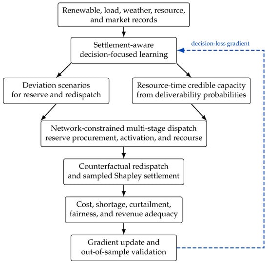
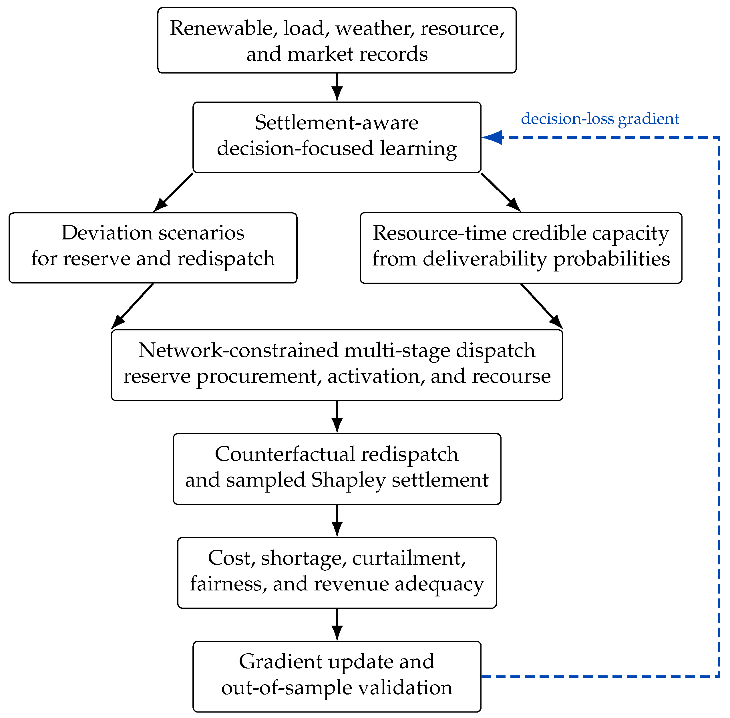
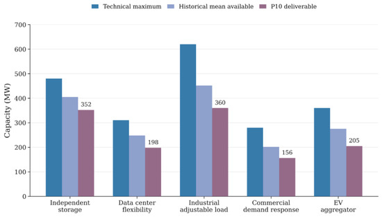
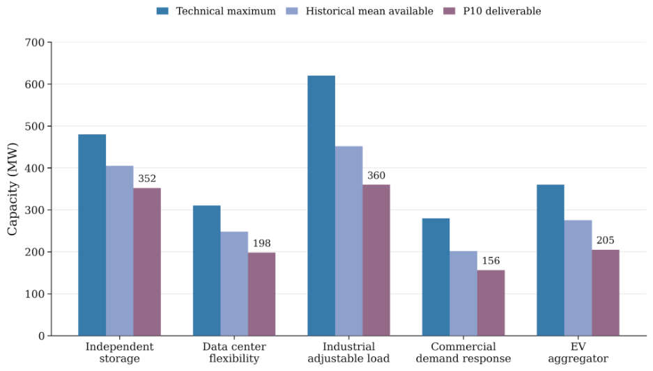
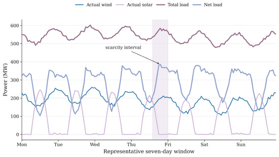
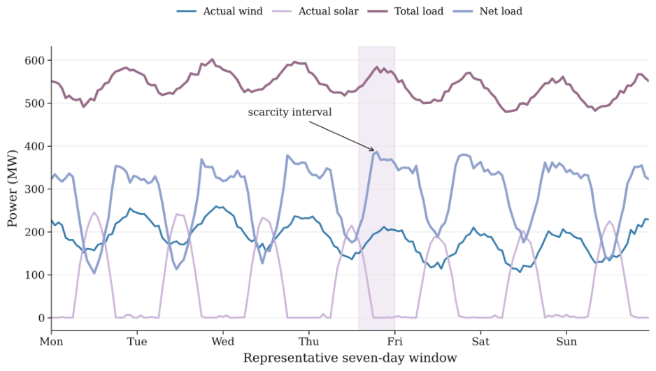
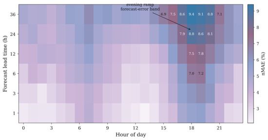
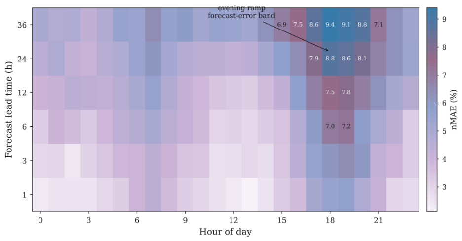
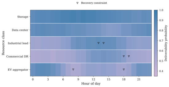
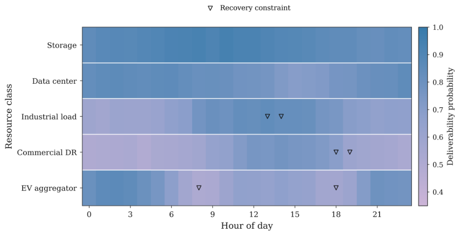
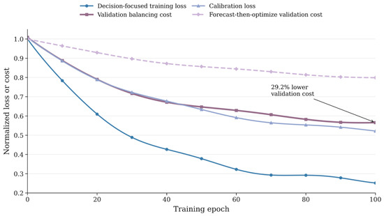
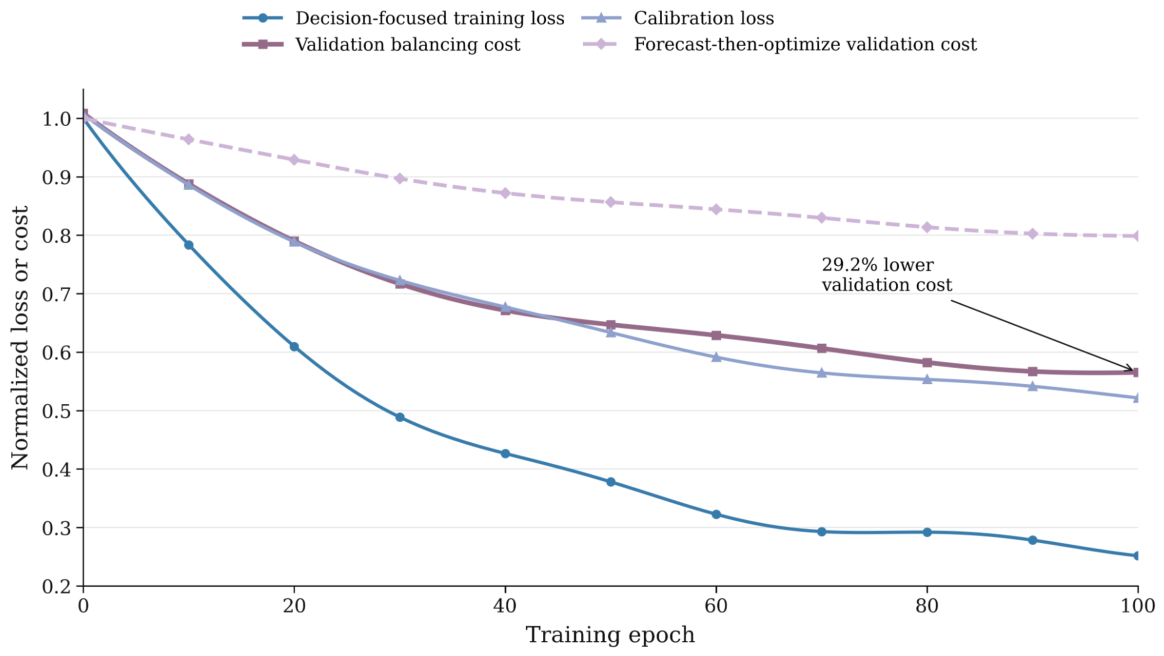
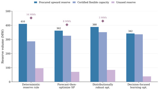
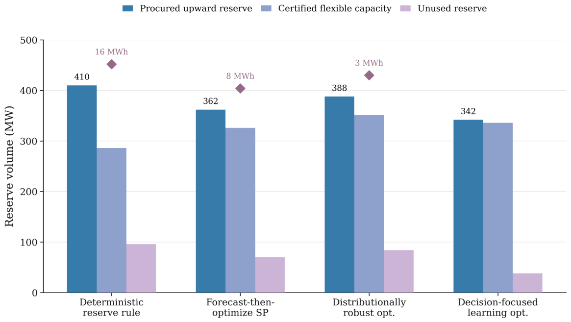
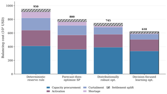
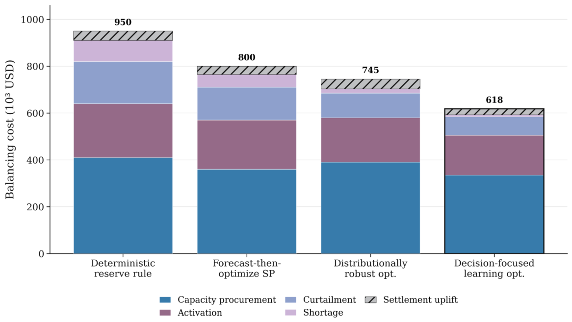
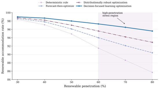
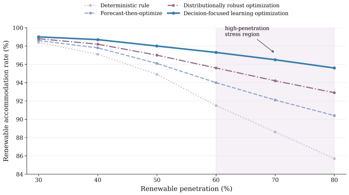
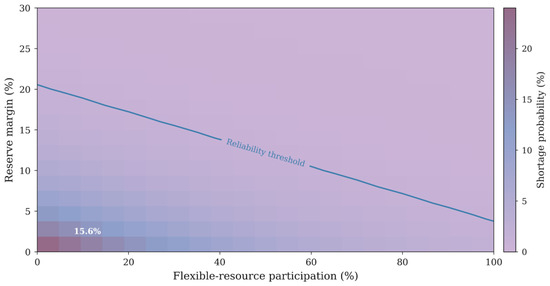
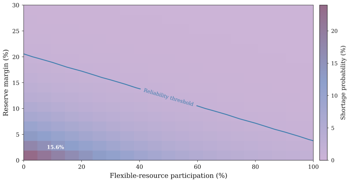
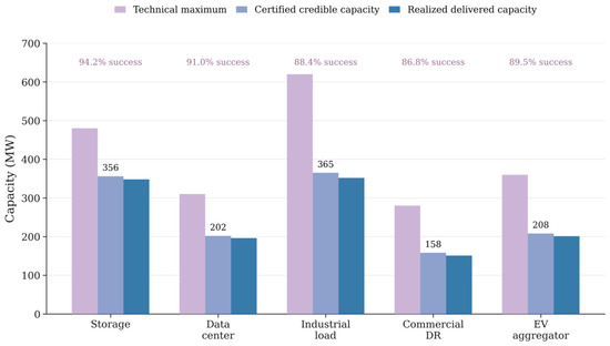
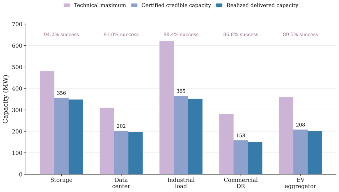
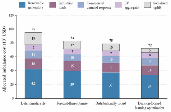
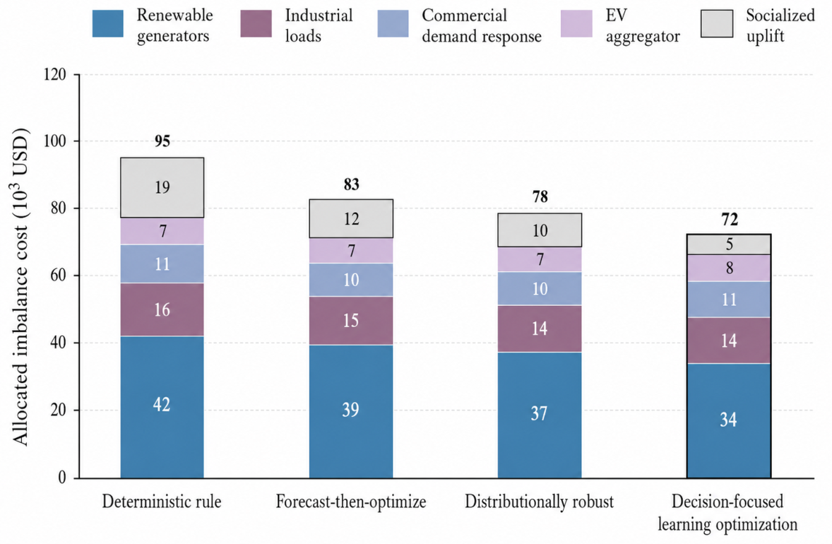
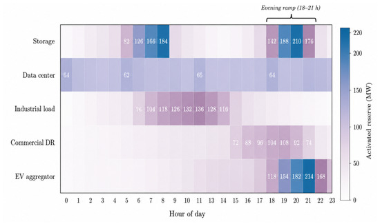
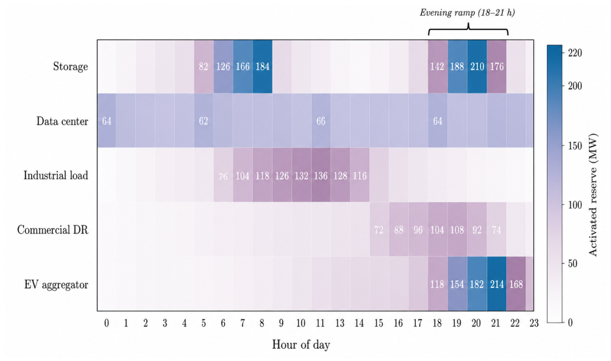
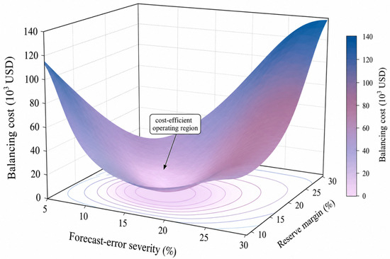
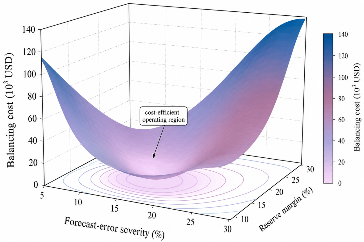
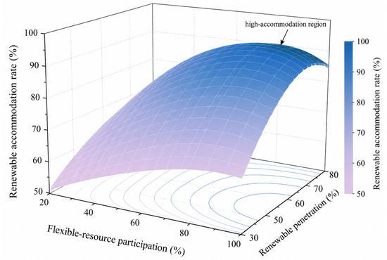
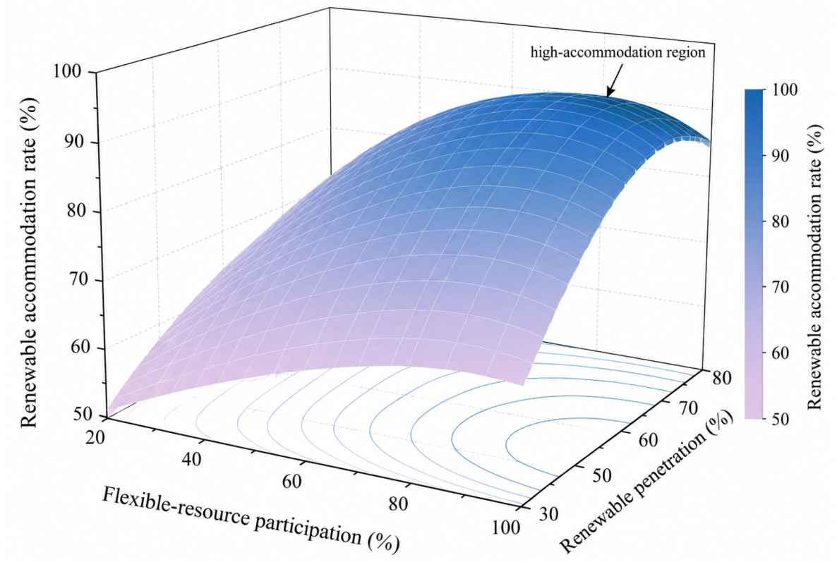
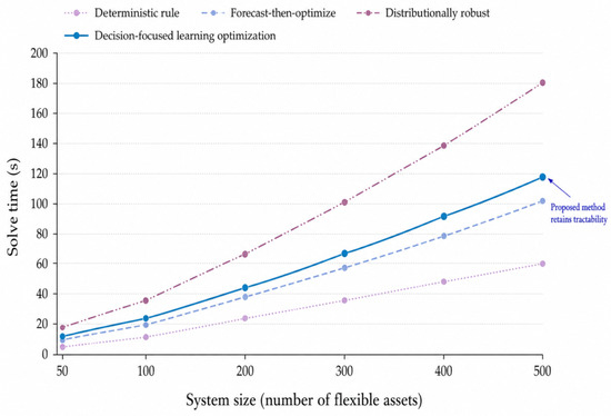
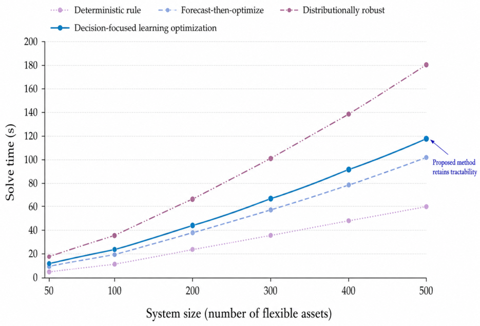
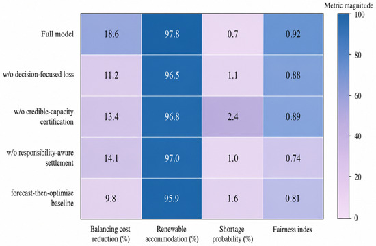
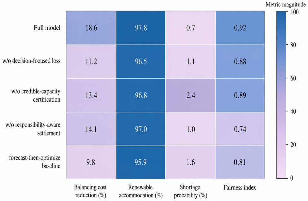

Disclaimer/Publisher’s Note: The statements, opinions and data contained in all publications are solely those of the individual author(s) and contributor(s) and not of MDPI and/or the editor(s). MDPI and/or the editor(s) disclaim responsibility for any injury to people or property resulting from any ideas, methods, instructions or products referred to in the content. |
© 2026 by the authors. Licensee MDPI, Basel, Switzerland. This article is an open access article distributed under the terms and conditions of the Creative Commons Attribution (CC BY) license.