A Computation-Oriented Bi-Layer Optimization for EV Scheduling Under Renewable Uncertainties via Information-Gap Decision Theory

Abstract

With the rapid penetration of electric vehicles (EVs) and renewable energy generation in distribution networks, the coordinated scheduling of flexible EV loads and uncertain renewable resources has become a critical research focus in modern power systems. This study investigates the collaborative optimal dispatch of thermal units, EVs, and renewable power generation. Different from conventional closed-loop game-based bi-level optimization, this paper constructs a transmission–distribution integrated scheduling framework and proposes a sequential hierarchical progressive optimization strategy for EV charging and discharging dispatch to fully tap the cross-level coordination potential of power grids. The upper transmission layer optimizes the joint operation of thermal units, wind power, and photovoltaic units to minimize the overall power supply cost, where the inequality power balance constraint is reasonably adopted to reserve power regulation margin for renewable fluctuation and meet practical engineering operation requirements. To effectively address the severe uncertainty of renewable power output without relying on accurate probability distribution information, information gap decision theory (IGDT) is employed to realize robust scheduling with risk-averse and opportunity-seeking decision adaptability. In the lower distribution layer, a theoretically grounded nodal electricity price (NEP) model integrating node loss sensitivity (NLS) and node load rate (NLR) is applied to substitute iterative power flow calculation, which realizes the spatial optimal allocation of EV charging and discharging nodes while significantly improving computational efficiency. The proposed framework comprehensively minimizes network power loss and user charging cost. Finally, extensive simulations based on the IEEE 33-node distribution system verify the effectiveness, computational superiority, and robustness of the proposed sequential hierarchical coordinated scheduling strategy.

1. Introduction

With climate change becoming increasingly prominent there is an urgent need to implement a green and sustainable development strategy [1]. At present, the government is gradually strengthening the support for renewable energy. Besides, electric vehicles (EVs) have attracted much attention because of their low consumption. One of the most effective ways to truly reduce the dependence on fossil fuels is to integrate and connect EVs and distributed power sources to the power grids, to maximize the use of clean energy [2].

For the renewable energy output fluctuation uncertainty problem, Ref. [3] proposes a stochastic planning model and by coordinating the complementary operation of system equipment to maximise the revenue. To handle the variability in the output of renewable energy, Ref. [4] established a robust optimal scheduling model whose goal is to minimize the total cost of the optimised system. Ref. [5] invoked the pseudo F-statistics metrics to determine the optimal scenarios after curtailment to deal with source-load uncertainty and improve the economic performance of microgrids. Ref. [6] creates a multi-objective ideal dispatch framework based on fuzzy chance-constrained planning to deal with wind power and load uncertainty, which is solved by combining with eddy-current search algorithm. Stochastic optimisation, robust optimisation and fuzzy optimisation are widely used in the previous studies to cope with the uncertainty problem, but they have the disadvantages of high computational difficulty and high data completeness requirement. Compared with the above optimisation methods, the information gap decision theory (IGDT) requires less information about the uncertainty quantities, can be quantitatively solved when both the probability distribution of the uncertainty quantities and the uncertain quantities are unknown, and can better deal with severe uncertainty scenarios [7]. Ref. [8] constructed an optimal allocation model for energy storage in distribution networks based on IGDT to address the adverse effects of renewable energy output as well as load demand uncertainty on distribution networks. Ref. [9] considered the impact of factors such as line reactive power loss and generator voltage magnitude on the stability of the distribution network. A combined scheduling model for generating units and a multi-objective reactive power planning model were created using IGDT to strengthen the distribution network. Ref. [10] developed a microgrid multi-temporal expansion planning model to solve the load growth uncertainty problem by using IGDT, but did not consider the impact of electric vehicle access. Refs. [11,12] used IGDT to solve the risk and revenue balancing problem of optimal multiple unit combinations for the uncertainty problem under the joint effect of multiple new energy units connected to a virtual power plant and distribution network, respectively.

The ordered charging scheduling strategies for the existing electric vehicles can be divided into centralised scheduling, decentralised scheduling and partitioned scheduling. The idea of centralised scheduling is simple and clear, and commonly used intelligent algorithms are used to solve the problem, including clustering algorithm [13], artificial fish swarm algorithm [14], and improved particle swarm algorithm [15,16], etc. However, the centralised control may increase the computing burden of the control centre, and increase the communication cost. Decentralised control transfers the computation from the control centre to each EV, which reduces the computational burden of the control centre introducing distributed algorithms [17], such as the alternating direction multiplier method, pairwise decomposition, etc., the original optimisation problem containing large EVs is decomposed into multiple optimisation problems containing only a single EV control variable. However, the decentralized control structure is relatively complex, and feasible solutions may not be obtained when solving the large-scale EVs scheduling problem. Zonal control handles EVs in zones, and common methods include setting up regional agents [18], which regulate different zones and upload scheduling information to the control centre, avoiding the shortcomings of centralised and decentralised scheduling. Ref. [19] propose a distributed strategy for managing the charging and discharging of electric vehicles. The findings indicate that we can utilize EVs for “peak shaving and valley filling” while also taking the grid’s and users’ interests into account, which will have implementation benefits. Ref. [20] examines demand-side response techniques based on pricing and incentives and suggests two EV load aggregator scheduling options: fixed contracting and flexible contracting. These strategies are optimized to maximize revenue and minimize load fluctuations. Ref. [21] describes the existing charging and discharging pricing strategies for EVs, and analyzes various coordinated charging and discharging models for EVs. Ref. [22] developed a multi-objective distributed optimization model that applies demand-side incentive response to consider the interests of the grid, load aggregators, and vehicle owners. The model breaks down the main objective into smaller, independent problems that are resolved through the use of the alternating direction multiplier method. Ref. [23] proposes an EV charging and discharging pricing strategy to establish a master-slave game model with smart cell operators and vehicle owners maximising their respective interests to achieve a win-win situation for operators and EV owners. Ref. [24] provides valuable insights for both short-term operational strategies and long-term infrastructure planning, ensuring that charging activities are aligned with the physical and economic constraints of the power system. The studies from Ref. [19] to Ref. [23] do not consider the impact of EV charging load on the distribution network in the spatial dimension, and the coordination between the power generation side and EV charging load.

In summary, the paper develops a computation-efficient bi-layer coordinated optimization scheduling framework for electric vehicle (EV) charging and discharging dispatch considering renewable generation uncertainty. Different from conventional scheduling methods that simply combine existing algorithms, this study first adopts an offline node loss sensitivity (NLS) calculation approach to quantitatively evaluate network power loss characteristics and further captures the real-time load saturation status of distribution network nodes via the node load rate (NLR). On this basis, a novel nodal electricity pricing (NEP) mechanism is established to realize spatial optimal allocation of EV charging resources and reduce grid operation loss. A transmission-distribution collaborative two-level scheduling model is constructed to achieve synergistic economic dispatch among thermal units, wind-photovoltaic renewables, and flexible EV loads. To address the stochastic and volatile nature of renewable power output, information gap decision theory (IGDT) is introduced to transform the deterministic scheduling model into a robust decision-making framework. The proposed model effectively balances minimum system operational cost and tolerable load fluctuation, while maximizing the accommodation range of uncertain renewable generation. Comprehensive case studies verify the technical superiority and engineering practicability of the proposed bi-layer optimization strategy. The optimized scheduling scheme minimizes the overall operational cost and resolves the inherent contradiction between system economic efficiency and operational stability. The research outcomes can provide valuable technical references for future multi-resource collaborative optimal dispatch of modern power systems with high penetration of renewables and electric vehicles.

The main academic and methodological innovations of this paper are summarized as follows:

Different from the above studies, this paper organically integrates transmission–distribution sequential hierarchical optimization, theoretically derived NLS-NLR joint nodal pricing, and IGDT uncertainty decision-making to form a systematic collaborative scheduling framework.

A data-driven nodal pricing model integrating node loss sensitivity (NLS) and node load rate (NLR) is proposed. Unlike the traditional empirical pricing methods, the proposed NEP is theoretically derived based on optimal power flow and marginal cost theory. It can dynamically guide the spatial migration of EV charging loads, effectively reduce distribution network loss, and avoid node overload or light-load imbalance problems.

This paper adopts the non-probabilistic IGDT to handle wind and photovoltaic output uncertainty, which overcomes the defects of high data dependence and poor robustness of traditional stochastic and robust optimization methods. Both risk-averse and opportunity-seeking decision-making models are established, which can flexibly balance system operational economy and anti-interference capability under extreme renewable fluctuation scenarios.

An offline NLS preprocessing method is introduced to avoid repeated power flow iterative calculation. The bi-layer decoupling optimization greatly improves the convergence speed and computational efficiency of the scheduling model, making the proposed strategy more suitable for real-time dispatch and large-scale grid engineering applications.

The remainder of this paper is organized as follows. In Section 2, the energy dispatch system model is described. The electric vehicle charging and discharging scheduling strategy based on Bi-layer optimisation is introduced in Section 3. Section 4 develops the IGDT model. Section 5 introduces simulation analysis, and Section 6 concludes.

2. Energy Dispatch System Model

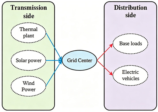
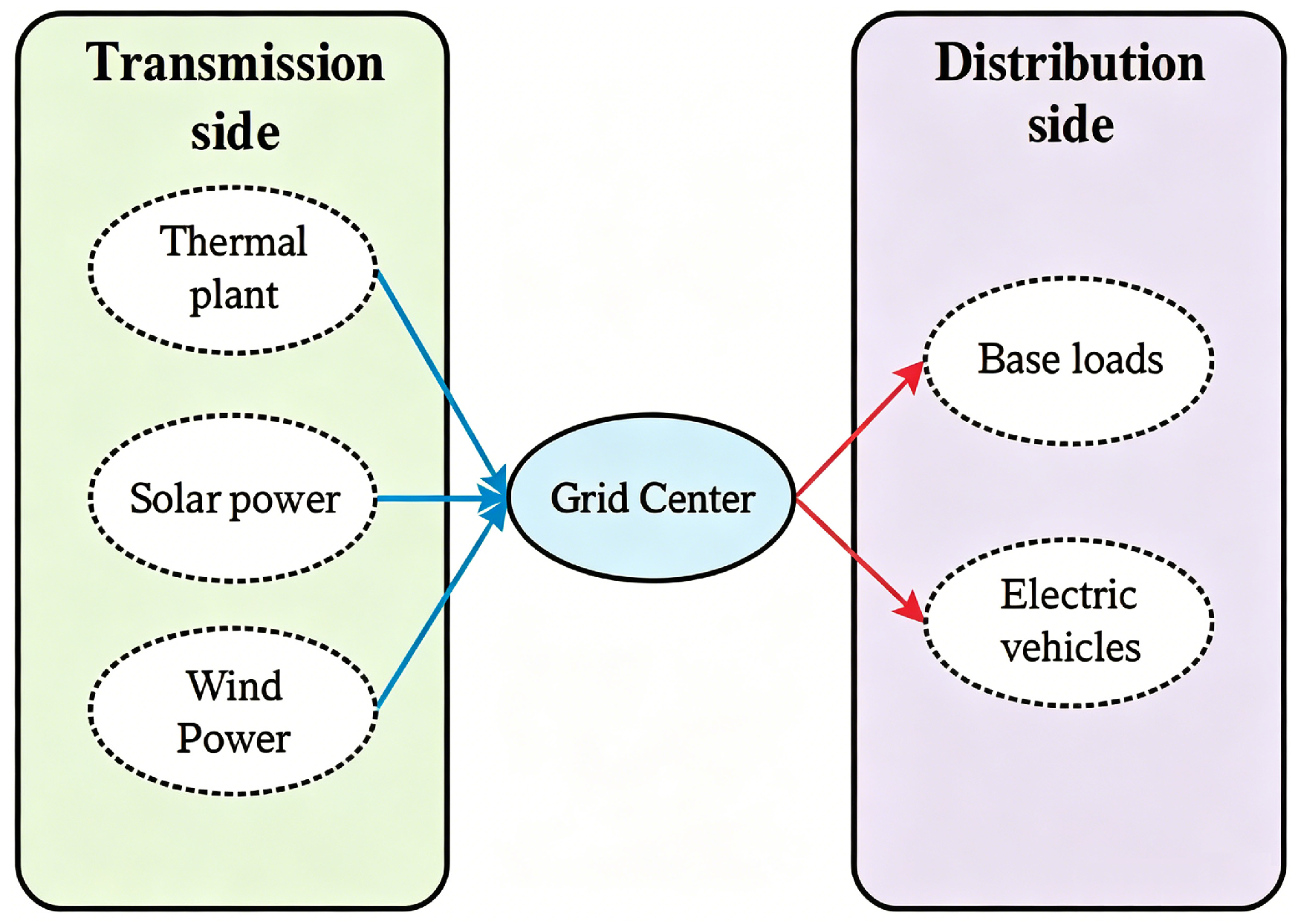
In this paper, the ESS structure is constructed as shown in Figure 1. Where ESS is divided into generation side and distribution side. The generation side consists of thermal plants, wind turbines and photovoltaics. The distribution side is electric vehicles and other base loads.

Figure 1. ESS system architecture.

2.1. Wind Power Model

The wind’s speed is a vital factor affecting wind power., and the current models for studying the variation of wind speed mainly include gamma distribution, Wilb distribution, Rayleigh distribution, etc. In this paper, the two-parameter Wilb distribution is used to describe the wind power model, and its probability distribution function expression is as follows:

$$f(v)={\displaystyle \frac{k}{\lambda }}({\displaystyle \frac{v}{\lambda }}{)}^{k-1}\cdot \exp [-({\displaystyle \frac{v}{\lambda }}{)}^k]$$

(1)

where v is the wind speed, k is the shape parameter, and λ is the scale parameter, which in general satisfies k > 0, λ > 0.

It is possible to represent the connection between wind power and wind speed as:

$$P_{WT}=\left\{\begin{array}{cc}0\hfill & v_s\le v_{in}\\ P_{wr}{\displaystyle \frac{v_s-v_{in}}{v_r-v_{in}}}\hfill & v_{in}\le v_s\le v_r\\ P_{wr}\hfill & v_r\le v_s\le v_{out}\\ 0\hfill & v_{out}\le v_r\end{array}\right.$$

(2)

where Pw and Pwr are the output power and rated power of the wind turbine, respectively; Vs and Vr are the actual wind speed and rated wind speed, respectively; Vs and Vout are the wind speed during cut-in and cut-out, respectively.

2.2. Photovoltaic Power Generation Model

PV power output is mainly influenced by photoelectric control, ambient temperature, and light intensity conversion efficiency and other factors. The PV power output equation in this paper’s model is as follows, with the only variables considered to be impacting the PV power output being the intensity of light radiation and the ambient temperature:

$$P_{PV}={\displaystyle \frac{P_{stc}\cdot I_t[1+k(T_t-T_{stc})]}{I_{stc}}}$$

(3)

$$T_t=T_{env,t}+{\displaystyle \frac{30I_t}{1000}}$$

(4)

where P_PV and P_stc are the real power output and rated power of PV power generation; I_t and I_stc are the intensity of light radiation and rated radiation intensity; k is the power temperature coefficient; T_t and T_stc are the current actual temperature and rated temperature of PV panels; T_env,t is the environment’s temperature at that moment.

3. Electric Vehicle Charging and Discharging Scheduling Strategy Based on Bi-Layer Optimisation

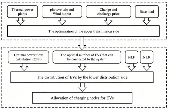
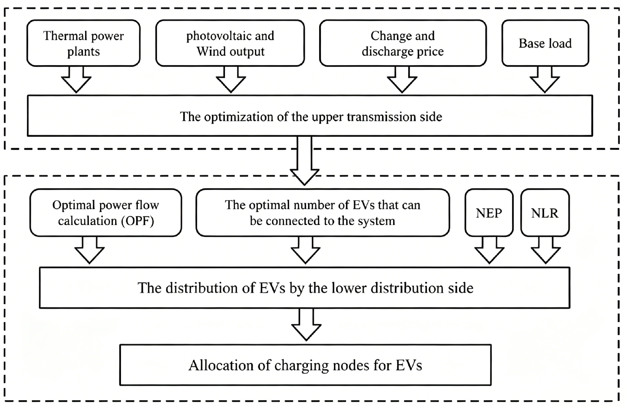
In order to achieve EV scheduling in both time and space dimensions, a bi-layer scheduling strategy is introduced in this thesis. In the upper layer optimal scheduling, the objective is to minimise the expense of running the electricity infrastructure and discharging and charging electric vehicles so as to maximize the ESS’s bonuses. The optimal number of EVs to be charged and discharged in each time slot can be obtained by considering factors such as generating units, wind farms, photovoltaic plants, and base load. The lower level scheduling then allocates the charging and discharging locations of EVs within the distribution system. When analysed using trend calculations, the amount of calculations increases and the grid is not able to provide timely tariff information to EVs.

Therefore, this paper analyses the effectiveness of every node inside the distribution network and suggests NLS and NEP as ways to cut down on computational labor. NLS can be obtained by offline computation and reduces the complexity in calculating the grid losses. NEP varies with time as well, which can direct the participation of EV in the scheduling in terms of time and space. The objective function is to minimise the grid loss and charging fees under NEP and to optimally allocate EV chargingnodes. In this work, the scheduling solution is implemented in a clear stepwise and progressive manner. The structural model of the scheduling strategy is shown in Figure 2.

Figure 2. The structural model of the bi-layer scheduling strategy.

3.1. Modelling of Upper-Layer Optimal Scheduling Strategy

Considering the unpredictability of solar and wind energy production, IGDT is invoked in this paper for analysis. At the transmission system level, in order to coordinate the timely charging and discharging of EV loads using the power output of generating units, wind, and photovoltaic power to achieve the optimal effect, a day-ahead scheduling strategy of the unit combination model is proposed, with the optimisation variables being the output of the units and the quantity of EVs charging throughout each time interval.

3.1.1. Objective Function of Upper-Layer Optimal Scheduling Strategy

Lowering operational expenses, emissions, charging and discharge costs, and system power shortage losses is the goal function of top layer scheduling.

(1) TPs power generation cost

$$C_{i,t}\left(P_{i,t}\right)=a_i{\left(P_{i,t}\right)}^2+b_i\left(P_{i,t}\right)+c_i$$

(5)

where Ci,t is the fuel expenditure for unit i at time t, and are the coefficients of the gasoline prices characteristic curve for unit i. Pi,t is the active power output of generating unit i at time t.

(2) Emission cost

$$C{\mathrm{e}}_{\mathrm{i},\mathrm{t}}(P_{i,t})=\beta \cdot [{\mathrm{aa}}_{\mathrm{i}}{(P_{i,t})}^2+{\mathrm{bb}}_{\mathrm{i}}(P_{i,t})+{\mathrm{cc}}_{\mathrm{i}}]$$

(6)

where, Cei,t(Pi,t) is the emission cost of generating unit i, aa_i, bb_i and cc_i are the coal consumption characteristic coefficients of unit i, and β is the emission cost parameter.

(3) Charging Costs

$$Cc{d}_t=-p_{c,t}{P}_{c,t}+p_{d,t}{P}_{d,t}$$

(7)

where Ccd_t is the charging cost of EVs in time period t; p_c,t and p_d,t are the charging and discharging electricity price of EVs in time period t; P_c,t and P_d,t represent the charging and discharging power of EVs in time period t, respectively.

(4) Insufficient of ESS electricity

$$Cp{s}_t=-\theta \left(P_{ld,t}+P_{c,t}-P_{W{T}_t}-P_{P{V}_t}-P_{T{P}_t}-P_{d,t}\right)$$

(8)

where Cps_t is the system energy shortage cost at time t and P_ld,t is the system base load; P_WT,t and P_PV,t represent the wind and photovoltaic power outputs at time t, respectively.

To summarize, the top-layer scheduling’s objective function is provided as:

$$min{\displaystyle \sum _{t=1}^T{\displaystyle \sum _{i=1}^4\left[C_{i,t}\left(P_{i,t}\right)+C{e}_{i,t}\left(P_{i,t}\right)+Cc{d}_t+Cp{s}_t\right]}}$$

(9)

where T is the total number of optimisation periods, in this paper we take 15 min as a period and T is 96.

3.1.2. Constraints of Upper-Layer Optimal Scheduling Strategy

The limitations include those related to the equipment, output, power balance, etc. The following requirements need to be met for every time interval t.

(1) Output and rate constraints:

$$P_i^{\min }\le P_{i,t}\le P_i^{\max }$$

(10)

$$R_{\mathrm{d},i}\le R_{t,i}\le R_{\mathrm{u},i}$$

(11)

where p_i^min and p_i^max are the lowest and highest values of the active output of generating unit i, respectively. R_d,i and R_u,i are the maximum downward and maximum upward adjustments of the active output of generator set i in a single time period, respectively.

(2) PV and Wind power constraints:

$$0\le P_{\mathrm{WT},\mathrm{t}}\le P_{WT,t}^{max}$$

(12)

$$0\le P_{\mathrm{PV},\mathrm{t}}\le P_{PV,t}^{max}$$

(13)

where $P_{PV,t}^{max}$ and $P_{PV,t}^{max}$ are the peak PV and wind output values at time t, respectively.

(3) Power balance

$$P_{ld,t}+P_{c,t}-P_{W{T}_t}-P_{P{V}_t}-P_{i,t}-P_{d,t}\ge 0$$

(14)

Facing strong uncertainties of wind and photovoltaic power, inequality power balance reserves adjustable power margin for fluctuation of renewable energy, which avoids infeasibility of scheduling results under extreme volatile scenarios.

(4) EV restraints:

$$0\le P_{c,t}\le P_{\mathrm{c}}^{\max }$$

(15)

$$0\le P_{\mathrm{d},t}\le P_{\mathrm{d}}^{\max }$$

(16)

$$E_{min}\le E_t\le E_{max}$$

(17)

$$E_{t+1}=E_t+\tau \left({\eta }_c{P}_{c,t}-{\displaystyle \frac{P_{d,t}}{{\eta }_d}}\right)$$

(18)

$$E_T=E_{max}$$

(19)

Equations (15)–(19) represent the EV energy constraints. The EV must be fully charged after the scheduling is completed. Where, Et is the EV’s capacity during time t, and Emin and Emax are the minimum and maximum EV capacity. τ is the length of the time slot. η_c and η_d are the EV charging and discharging efficiencies.

3.2. Modelling of Lower Level Optimal Scheduling Strategy

The tidal current distribution issue caused by EVs connecting to every regional distribution network node must be taken into account by the lower layer optimization technique. This research proposes a lower layer optimization scheduling technique at the distribution network level under the existing NEP system, based on the optimum current. The overall charging and discharging loads of EVs are efficiently distributed to each distribution network node by optimizing the current distribution.

3.2.1. Nodal Electricity Price

In practical power grid operation, individual EV users only make charging decisions based on their own travel demands and economic costs, without considering real-time grid operating parameters or power flow conditions, which renders passive and uncoordinated EV charging scheduling. To address this issue and realize grid-friendly EV integration, this study reconstructs a rigorous nodal economic pricing (NEP) model grounded in power flow theory and microeconomic marginal cost principles, rather than adopting the heuristic empirical formulation in the preliminary version. The refined NEP mechanism fully incorporates two core nodal imbalance indicators, namely nodal load residue (NLR) and nodal load surplus (NLS). Through standardized theoretical derivation and mechanism analysis, the inherent coupling relationship between NLS/NLR power imbalance characteristics and dynamic nodal pricing is quantitatively clarified, which realizes scientific and reasonable grid economic dispatch and guides the active participation of EVs in optimal scheduling.

(1) NLS

Grid losses occur when electric vehicles are charged and discharged via the grid. The efficiency of real-time EV scheduling will suffer when different loads are allocated to each node and the ideal tidal current is directly computed, adding complexity to the optimization process. The number of grid losses resulting from an increase in a grid node’s per-unit load is represented by NLS. The following is the formula:

$${\mathrm{NLS}}_m={\displaystyle \frac{\partial L}{\partial P}}$$

(20)

where NLSm denotes the loss sensitivity of the grid at node m, L is the grid loss, and P indicates the active power at the node.

(2) NLR

Focusing solely on decreasing grid losses can result in nodes experiencing either heavy or light loads that impact the grid’s peaking capability. NLR denotes the proportion of an individual node’s actual load versus its maximum capacity and facilitates the evaluation of a node’s load balance. The given expression illustrates NLR:

$${\mathrm{NLR}}_{m,t}={\displaystyle \frac{P_{m,t}}{P_m^{\max }}}$$

(21)

where NLR_m,t denotes the load factor of node m during time slot t, P_m,t is the node m’s overall load in time slot t, and P_m^max indicates the highest load that node m can support.

This paper makes the claim that the grid’s operational state remains constant throughout a single dispatch time, with an unvarying tariff during each period. Consequently, NLS and NLR are merged, and the two dimensions of evaluation indices undergo normalization and linear weighting:

$${\mathsf{\Gamma }}_{m,t}={\omega }_1{\mathrm{NLS}}_{m,t}+{\omega }_2{\mathrm{NLR}}_{m,t},{\omega }_1+{\omega }_2=1$$

(22)

When the lowest possible cost of energy is taken into account, NEP is defined as:

$${\mathrm{NEP}}_{m,t}={\mathrm{NEP}}_{\mathrm{base},t}+{\mathsf{\Gamma }}_{m,t}{P}_{m,t}$$

(23)

where NEP_base,t represents the fundamental charge for the designated time period t.

3.2.2. Objective Function of Lower Level Optimal Scheduling Strategy

Lower scheduling seeks to reduce EV charging costs as well as the NEP system’s grid node loss.

(1) Grid Losses

$$L_{m,t}={\mathrm{NEP}}_{m,t}\times {\mathrm{NLS}}_{m,t}{P}_{m,t}$$

(24)

(2) Charging Costs for EVs under the NEP

$$C{n}_{m,t}={\mathrm{NEP}}_{m,t}\cdot \tau \left(Nch{g}_{m,t}{P}_c-Ndi{s}_{m,t}{P}_d\right)$$

(25)

where Nchgm,t and Ndism,t indicate the amount of EVs have been charged and discharged at node m at time t, respectively.

The lower level optimum scheduling strategy’s objective function may be defined as:

$$\min {{\displaystyle \sum }}_{t=1}^T{{\displaystyle \sum }}_{m=1}^{32}[{\omega }_3{L}_{m,t}+{\omega }_{4}C{n}_{m,t}],{\omega }_3+{\omega }_4=1$$

(26)

3.2.3. Constraints of Lower Level Optimal Scheduling Strategy

(1) Voltage Constraints

The voltage at each node needs to be within the maximum and minimum voltage allowed for that node:

$$V_{\min }\le V_{m,t}\le V_{\max }$$

(27)

where Vmin and Vmax are the lower and upper limits of the voltage at node m.

(2) The amount of EVs being charged and discharged

The total amount of EV charging during each time period must correspond to the quantity of electric vehicle charging during that time period determined by the upper-level optimization.

$${{\displaystyle \sum }}_{m=1}^{32}N{c}_{m,t}=Nch{g}_t$$

(28)

$${{\displaystyle \sum }}_{m=1}^{32}N{d}_{m,t}=Ndi{s}_t$$

(29)

where Ncm,t and Ndm,t denote The quantity of electric vehicles at node m that were charged and discharged during time t.

(3) Number of charging stations

$$0\le N{c}_{m,t}\le Ncma{x}_{m,t}$$

(30)

$$0\le N{d}_{m,t}\le Ndma{x}_{m,t}$$

(31)

$$N\mathrm{c}ma{x}_{m,t}={\displaystyle \frac{Mc}{NL{R}_{m,t}}}$$

(32)

$$Ndma{x}_{m,t}={\displaystyle \frac{Md}{NL{R}_{m,t}}}$$

(33)

where Ncmax_m,t and Ndmax_m,t represent the maximum number of EVs that can be charged and discharged by a node at time t. Mc and Md denote the limits for both maximum charging and maximum draining of EVs. A node’s maximum capacity to host EVs is inversely related to NLR.

4. IGDT Model

It should provide a concise and precise description of the experimental results, their interpretation, as well as the experimental conclusions that can be drawn.

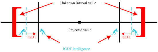
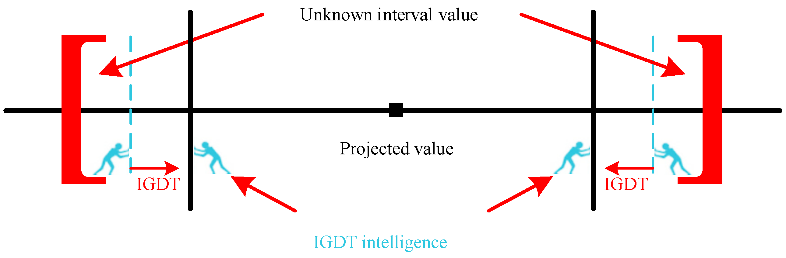
To address the issue of considerable uncertainty in wind power output within the upper level optimization strategy, this study applies IGDT to model such uncertainty within the upper layer model. IGDT is an interval optimization method that is non-probabilistic, enabling direct optimization of uncertain parameters in accordance with the desired objective, as well as analysis of their effects on the system. Figure 3 illustrates how IGDT manages uncertainty, with its two intelligences, risk aversion and opportunity seeking.

Figure 3. Schematic diagram of IGDT.

In this paper, the uncertainty in the wind and light output is modelled as shown in the following equation:

$$\left\{\begin{array}{l}U\left(\alpha ,{\tilde{P}}_t^{\mathrm{DG}}\right)=\left\{P_t^{\mathrm{DG}}:\mid {\displaystyle \frac{P_t^{\mathrm{DG}}-{\tilde{P}}_t^{\mathrm{DG}}}{{\tilde{P}}_t^{\mathrm{DG}}}}\mid ⩽\alpha \right\}\\ \alpha \ge 0\\ P_t^{\mathrm{DG}}=P_t^{\mathrm{PV}}+P_t^{\mathrm{WT}}\\ P_t^{\mathrm{DG}}\in U\left(\alpha ,{\tilde{P}}_t^{\mathrm{DG}}\right)\end{array}\right.$$

(34)

In the formula, U(α,$\tilde{P}$_t^DG) is the output unpredictability model for wind power; α is the un-certainty interval of output in the actual situation; P_t^DG is the uncertainty output in time period t; P_t^PV and P_t^WT are the uncertainty output of PV and wind power in time period t, respectively.

As previously stated, IGDT involves two decision-making approaches. Risk aversion aims to determine the optimal decision variables by minimizing uncertainty in IGDT maximisation. Conversely, chance involves seeking to reduce the value of the objective function in IGDT maximisation, with the aim of identifying the best set of decision variables. To lessen the effects of scenery uncertainty on the system’s operation, this paper analyses these two methods independently.

4.1. Robust IGDT Scheduling Model Based on Risk Aversion (OM)

This approach views fluctuations arising from uncertain parameters as detrimental because they lead to an escalation in the system’s scheduling expenses. Using the following formulation, the decision-maker maximizes the unknown parameter’s fluctuation range, given that the dis-patch cost limit does not surpass the accepted range:

The risk-averse optimization (OM) strategy is designed to hedge against adverse impacts brought by renewable power uncertainty. In this framework, parameter fluctuations are regarded as detrimental factors that may increase system scheduling costs. To guarantee the operational robustness of the power system, the decision-maker aims to maximize the allowable fluctuation boundary of uncertain renewable parameters while ensuring that the system scheduling cost does not exceed the pre-set acceptable cost threshold. The complete mathematical formulation of the risk-averse IGDT model is presented in Equation (35):

$$\left\{\begin{array}{l}\max \alpha \\ s.t.\left\{\begin{array}{l}f=\underset{X}{min}{\displaystyle \sum _{t=1}^T{\displaystyle \sum _{i=1}^4\left[C_{i,t}\left(P_{i,t}\right)+C{e}_{i,t}\left(P_{i,t}\right)+Cc{d}_t+Cp{s}_t\right]}}\\ s.t.\left\{\begin{array}{l}\max f(X,P_t^{\mathrm{DG}})\text{<}{f}^{\prime }\\ f^{\prime }=(1+\beta )f_0\\ h(X,P_t^{\mathrm{DG}})=0\\ g(X,P_t^{\mathrm{DG}})\ge 0\\ P_t^{\mathrm{DG}}\in U\left(\alpha ,{\tilde{P}}_t^{\mathrm{DG}}\right)\\ 0\le \alpha \le 1\\ 0\le \beta \le 1\end{array}\right.\end{array}\right.\end{array}\right.$$

(35)

where f represents the value of the objective function in the upper model, X denotes the decision variable, f′ represents the maximum objective function that the decision maker can afford after considering uncertainties, β is the bias factor established by the decision maker, f₀ denotes the optimal objective function value under the deterministic model, and h(X,P_t^DG) and g(X,P_t^DG) ≥ 0 respectively represent the equality constraints and inequality constraints.

4.2. Risk Pursuit Based Opportunity IGDT Scheduling Model (RM)

Different from the risk-averse OM model, the risk-pursuing opportunity optimization (RM) model fully exploits the beneficial potential of renewable power fluctuations. This strategy treats reasonable parameter fluctuations as favorable factors that can reduce overall system dispatch costs. The core optimization goal of the RM model is to minimize the fluctuation range of uncertain renewable parameters on the premise that the actual scheduling cost is lower than the expected reference cost, so as to obtain the optimal output of each generation unit and EV scheduling scheme. The standardized and complete formulation of the risk-pursuing IGDT model is established in Equation (36):

$$\left\{\begin{array}{l}\min \alpha \\ s.t.\left\{\begin{array}{l}f=\underset{X}{min}{\displaystyle \sum _{t=1}^T{\displaystyle \sum _{i=1}^4\left[C_{i,t}\left(P_{i,t}\right)+C{e}_{i,t}\left(P_{i,t}\right)+Cc{d}_t+Cp{s}_t\right]}}\\ s.t.\left\{\begin{array}{l}\min f(X,P_t^{\mathrm{DG}})<f^{\prime }\\ f^{\prime }=(1-\beta )f_0\\ h(X,P_t^{\mathrm{DG}})=0\\ g(X,P_t^{\mathrm{DG}})\ge 0\\ P_t^{\mathrm{DG}}\in U\left(\alpha ,{\tilde{P}}_t^{\mathrm{DG}}\right)\\ 0\le \alpha \le 1\\ 0\le \beta \le 1\end{array}\right.\end{array}\right.\end{array}\right.$$

(36)

Consistent with the unified notation rule, all parameters in Equation (36) follow the above definitions. The RM model focuses on capturing the economic benefits brought by renewable power deviation, forming a complementary scheduling mechanism with the OM model. The dual IGDT models jointly realize the adaptive scheduling of power systems under different renewable fluctuation scenarios, effectively balancing system operational risk and economic performance.

4.3. Model Solving Strategy

The IGDT solution process is shown in Algorithm 1.

Algorithm 1. The IGDT process

Input: Genset parameters, wind power output forecasts, photovoltaic power forecasts, load data. Initializing the baseline values: Calculate the optimal value of the objective function based on the upper level optimal dis-patch model on the transmission side. Selecting an IGDT Strategy: If risk_avoidance_strategy == true:   Setting risk aversion factors.   Solve the IGDT robust scheduling model ac-cording to Equation (35). else:   Setting the chance level factor.   Solve the IGDT opportunity scheduling model according to Equation (36). Output: The uncertainty radius of the uncertain parameters and the corresponding possible costs.

5. Simulation Analysis

It should provide a concise and precise description of the experimental results, their interpretation, as well as the experimental conclusions that can be drawn.

This section includes simulations to confirm the suggested bi-level scheduling strategy’s efficacy. This section evaluates using a 3.2 GHz Intel Pentium PC with 16 GB RAM with Matlab 2021b. The parameters used in the simulation of this paper refer to Ref. [24] and the wind and the PV and wind generation data is sourced from Ref. [25].

5.1. Simulation Analysis of the Upper Level of the Transmission Side

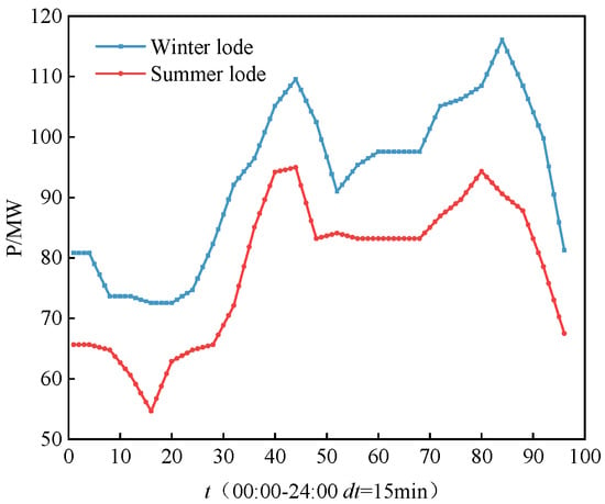
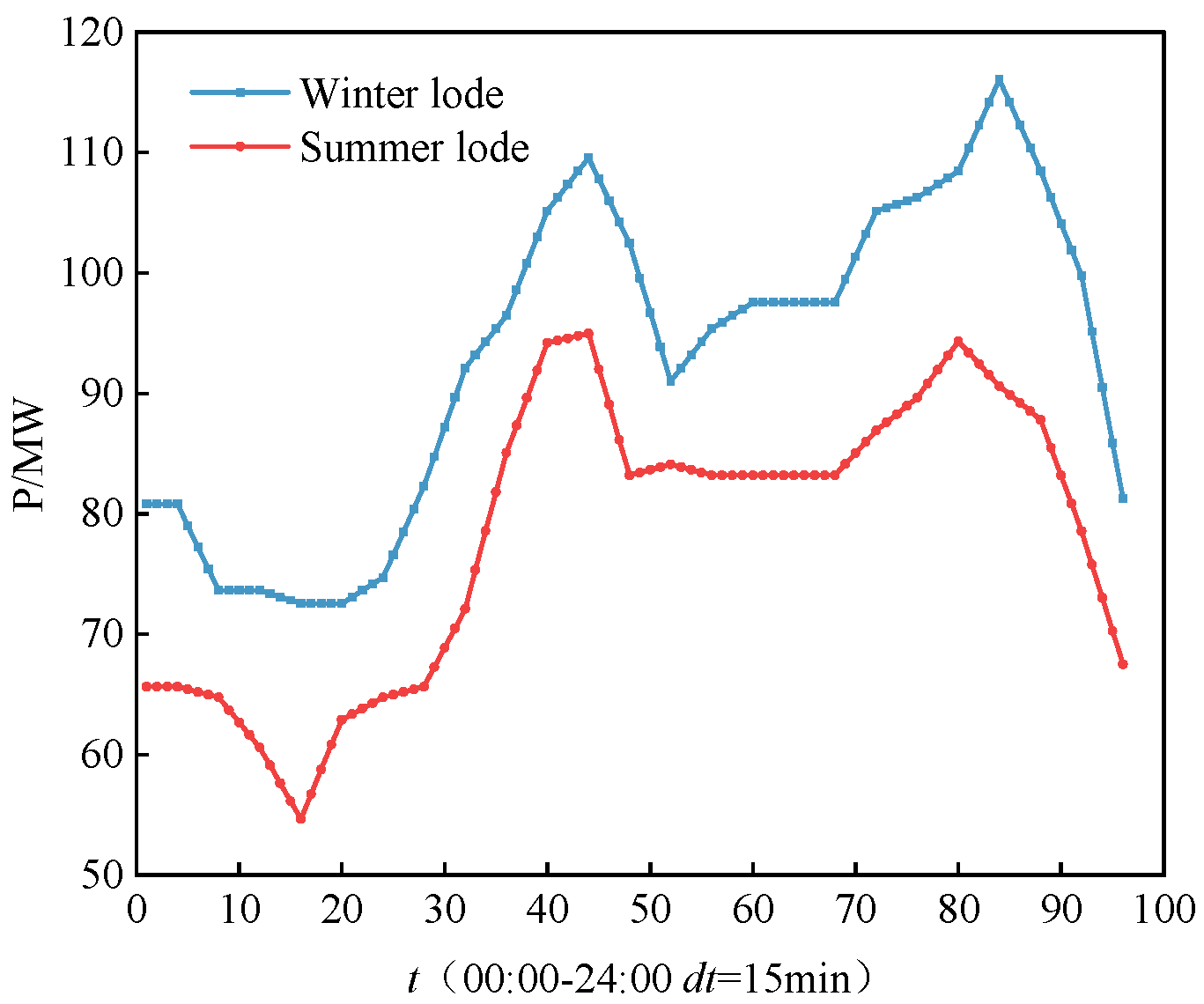
The upper level dispatches power generation to optimize the overall benefit of the ESS. By merging the ESS’s upper and lower limits for EV charging and discharging, the number of EVs to be charged or discharged during each time slot is determined to achieve the highest ESS benefit. Figure 4 displays the base load of the grid used in the upper layer simulation.

Figure 4. ESS system architecture Base load of the grid.

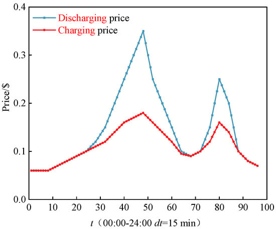
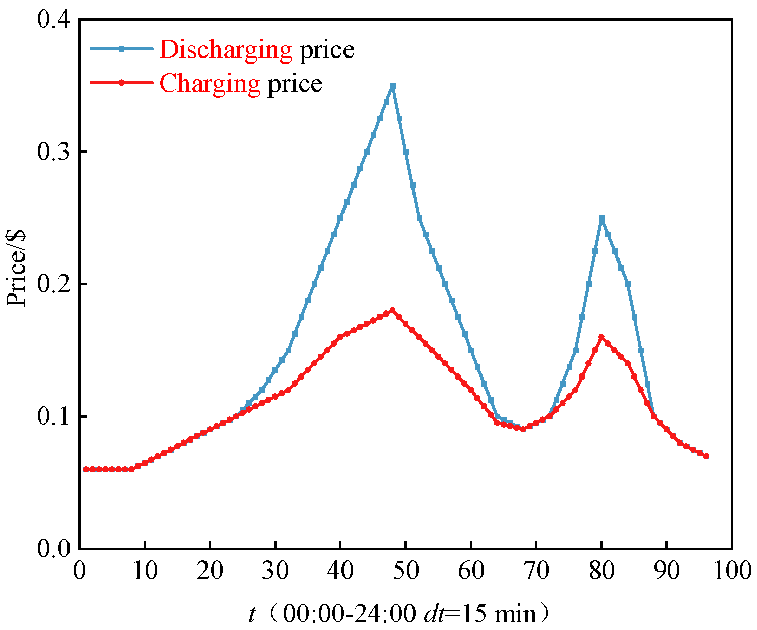
The Figures in Figure 5 illustrate the price, with higher price attributed to discharge to mitigate the accelerated ageing of the batteries.

Figure 5. Charging and discharging price.

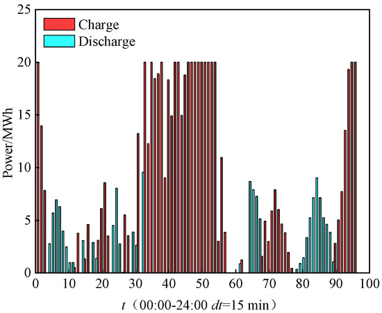
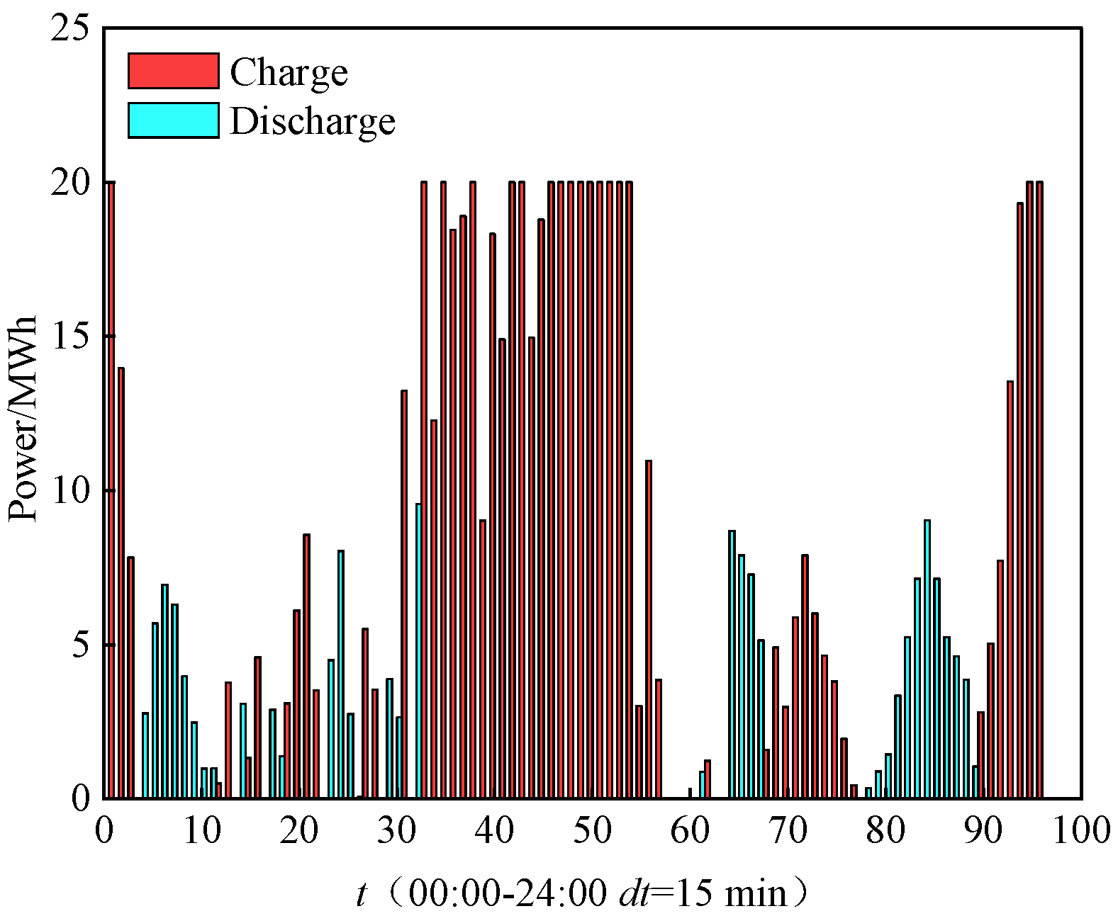
Figure 6 displays the EV’s capacity for charging and discharging per time slot. Upon arrival at the place of employment, the user connects the EV to the grid for charging between time slots 34 and 60. The EV is discharged from time slots 64 to 72, when commuters travel back home. EVs are charged during time slots 84 to 92 when commuters return home from work, resulting in the centralised charging and discharging of the vehicles. The quantity of EVs on the grid may be ascertained by computing the energy and power used for charging and discharging throughout each time interval.

Figure 6. Electric vehicle charging and discharging power.

Thermal power plants must contribute to power generation in order to meet the generation side’s power requirements. Table 1 exhibits pertinent parameters of the power-producing units.

Table 1. Generator set output parameters.

Unit Number	Maximum Output/MW	Minimum Output/MW	a	b	c
1	35	10	0.00048	16.19	100
2	30	0	0.00200	16.60	700
3	22	0	0.00712	22.26	370
4	20	0	0.00173	27.29	670

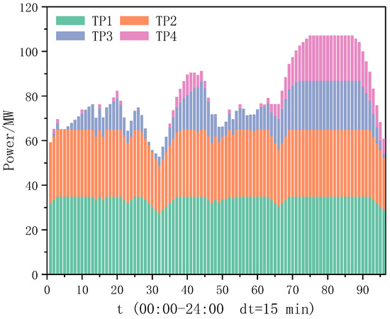
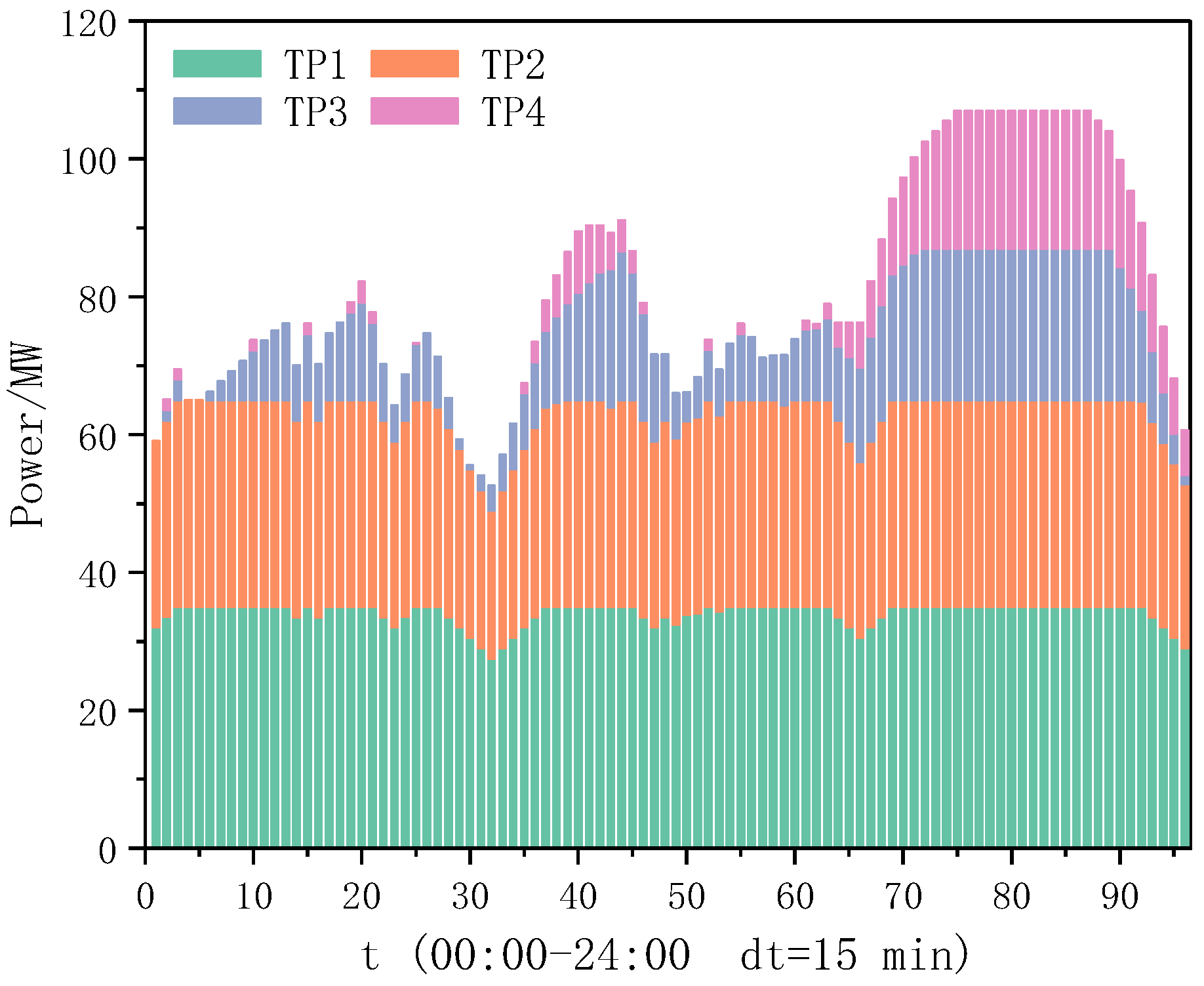
Table 1 presents the generation of electricity for each unit and its corresponding costs. The data in Table 2 enables the computation of the unit cost of electricity generated by four thermal power plants. Nonetheless, the average cost of charging an electric vehicle is 0.3431, which is comparatively lower than TP4’s cost. Thus, the creation of TP4 is not meant for EV charging; rather, it is meant to maintain the system’s power balance and avoid the excessive costs associated with power scarcity. The output conditions of the four thermal plants for each time slot are shown in Figure 7. Because of their low cost, it can be seen that TP1 and TP2 produce a significant amount of power within the permitted range, but TP3 pro-duces a somewhat lower output. TP4 has lowered its output from time slots 75 to 90 in order to provide a reliable power supply and adequate buffer.

Table 2. Unit Generation Cost.

Electricity Generator	Generated Electrical Energy/Mwh	Genertion Costs/k$	Emission Costs/k$
TP1	3264.0	372.28	6.852
TP2	2774.6	283.55	5.792
TP3	1199.0	151.38	2.467
TP4	551.3	119.13	1.376
PV	921.0	/	/
PP	811.8	/	/
EV	−483.0	−165.75	/

Figure 7. Output state of each time slot of the gen-erator set.

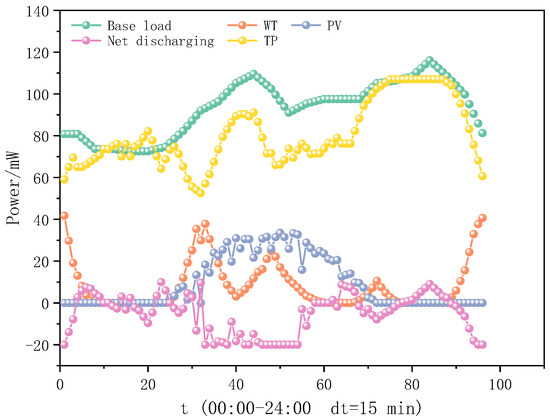
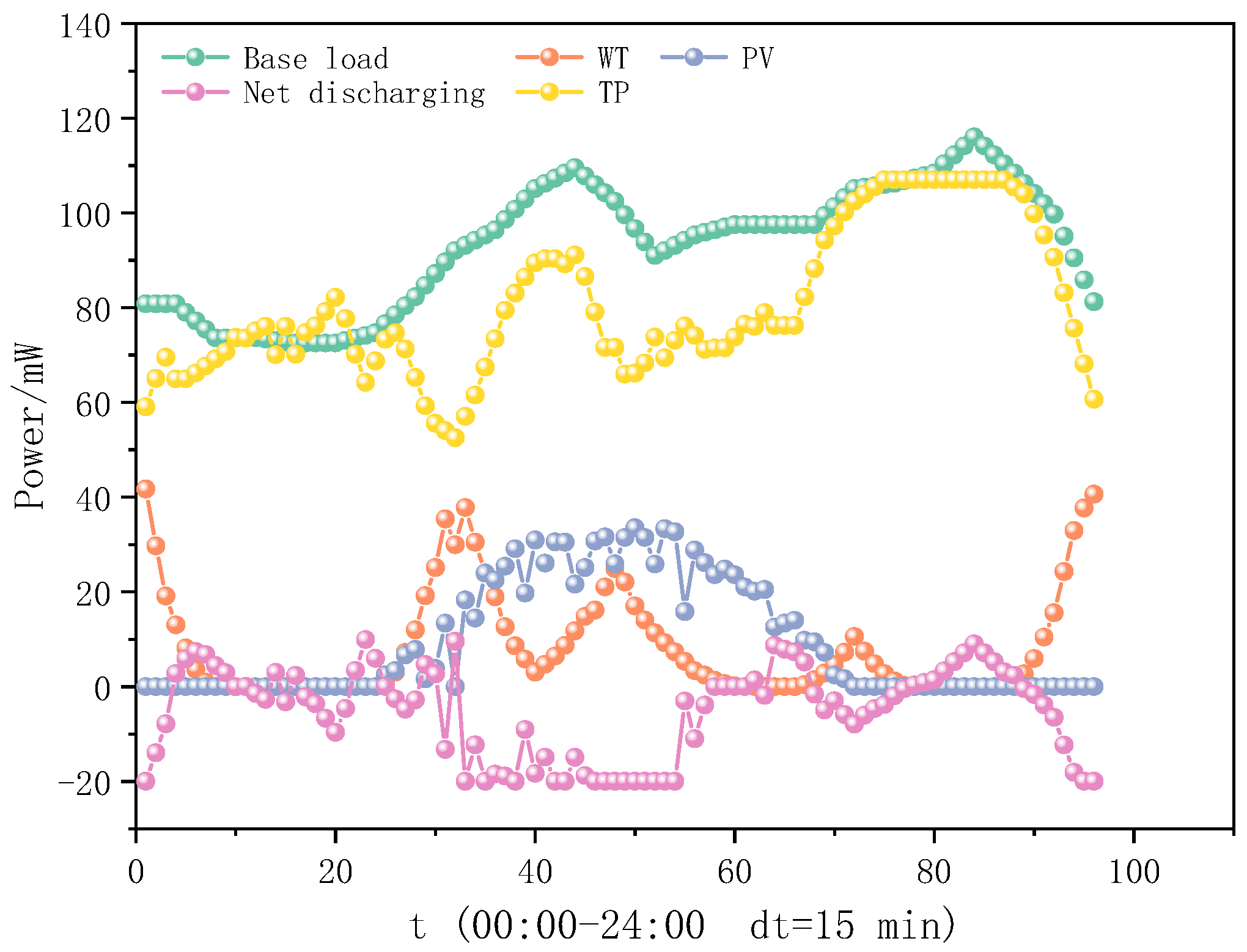
Figure 8 displays the output states of all units during each time slot. According to the Figure, there is never a power outage while the power system is scheduled. This indicates that the amount of power generated and consumed is equal. The time slots between 25 and 72 (6:00–18:00) witness a predominant concentration of PV generation, while wind generation is multi-modal and spread throughout the dispatch interval. The rates of wind and solar energy abandonment were 0.0% and 0.4%, respectively. Lack of absorptive capacity and wastage of re-sources result from the grid nodes’ inability to connect with more electric vehicles, causing the abandonment of renewable energy. This paper’s scheduling strategy allows for optimal use of renewable energy. Also, the peak of wind power generation typically coincides with the trough of thermal power plant generation. Thermal and renewable energy generation have a complementary relationship. Wind and photovoltaics are effectively utilised in the 35 to 60 time slots by the centralised charging of electric vehicles whilst wind is completely utilised during the 85 to 90 charging time slots.

Figure 8. Output status of each unit.

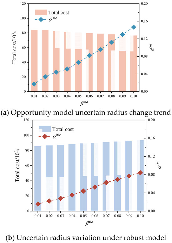
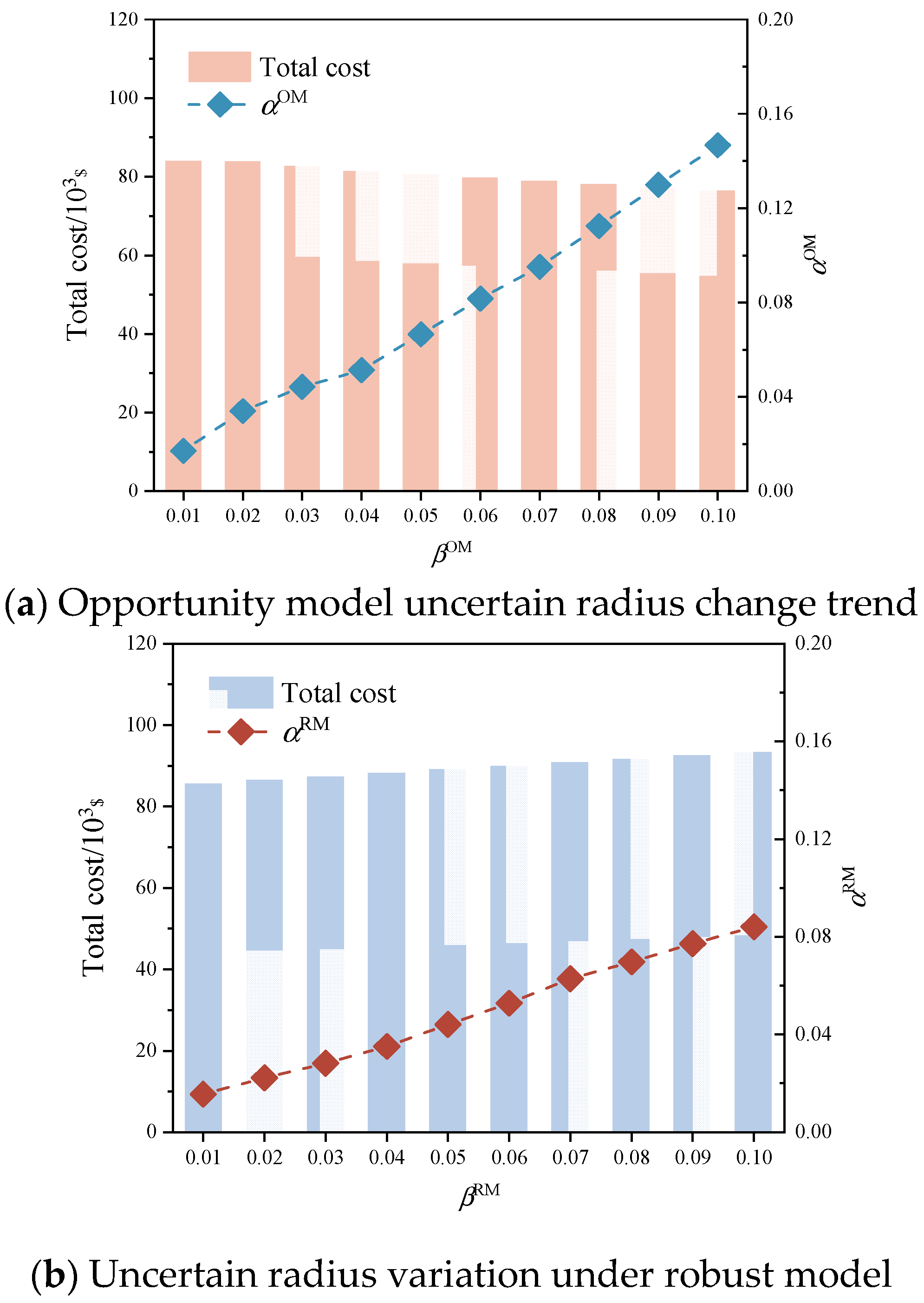
The above results validate the optimisation of ESS by EV access, but do not account for the ambiguity effects of wind and PV. The combined cost of optimal dispatch in the IGDT optimisation model is 4857 $. The cost deviation factors β^OM and β^RM have a variation range set to 0.01–0.10. Table 3 displays the uncertainty radius α and the total operating cost of OM and RM, while Figure 9 exhibits the trend of the uncertainty radius α and the total operating cost with the cost deviation factors β^OM and β^RM.

Table 3. OM and RM and Operating Costs.

βRM	βOM	RM		OM
		α	F	α	F
0.01	0.01	0.0156	85,573	0.0171	84,008
0.02	0.02	0.0222	86,463	0.0339	83,893
0.03	0.03	0.0282	87,325	0.0442	82,632
0.04	0.04	0.0351	88,250	0.0513	81,362
0.05	0.05	0.0441	89,100	0.0665	80,605
0.06	0.06	0.0528	89,948	0.0816	79,765
0.07	0.07	0.0628	90,795	0.0951	78,917
0.08	0.08	0.0697	91,646	0.1124	78,068
0.09	0.09	0.0772	92,494	0.1299	77,220
0.10	0.10	0.0841	93,343	0.1467	76,371

Figure 9. Trend of α and total operating cost with deviation factor.

From Figure 9, it is evident that, in OM, the desired target value steadily decreases as the decision maker-formulated cost deviation factor, β^OM, increases. Simultaneously, the total operating cost obtained through model optimisation gradually decreases and the radius of uncertainty, α, generally increases. This happens because the OM decision-maker thinks ambiguity will have a beneficial effect. and the actual value trends towards a favourable direction regarding target expectations. The potential advantages from the wind and light output uncertainty are more important the bigger the uncertainty radius; this might lead to further benefits and a reduction in overall operating expenses. The potential advantages from the wind and light output uncertainty are more important the bigger the un-certainty radius; this might lead to further benefits and a reduction in overall operating expenses. The potential advantages from wind and light output uncertainty are more important the bigger the uncertainty radius; this might lead to further benefits and an α drop in overall operating costs.

The total operating cost can be decreased or kept at the decision maker’s desired target value (1 − β^OM) × F₀ whenever it varies within [(1 − α) $\tilde{P}$_t^DG, (1 + α) $\tilde{P}$_t^DG], due to the impact of the surrounding environment.

5.2. Simulation and Analysis of Lower Distri-Bution Side

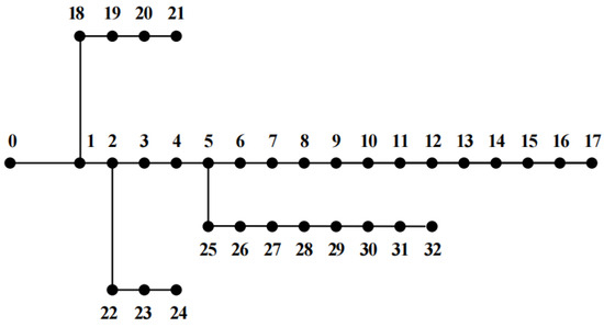
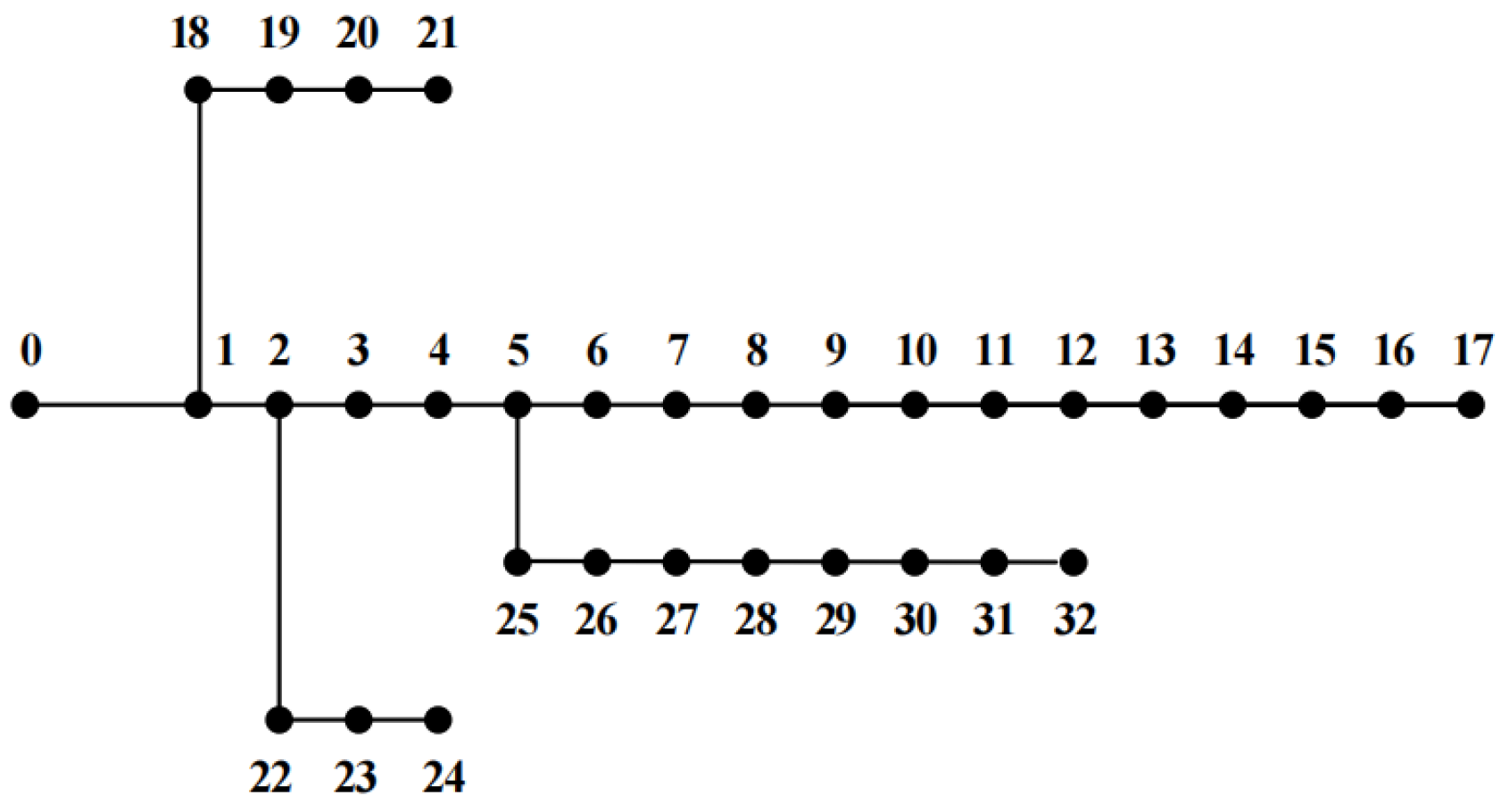
The lower layer simulation is based on the IEEE 33-node as shown in Figure 10. Node 0 is used as a balancing node. The access nodes for charging and discharging EVs acquired from the top layer scheduling are assigned by the bottom layer scheduling simulation using NEP.

Figure 10. IEEE33 Node Network Topology Diagram.

5.2.1. NLS

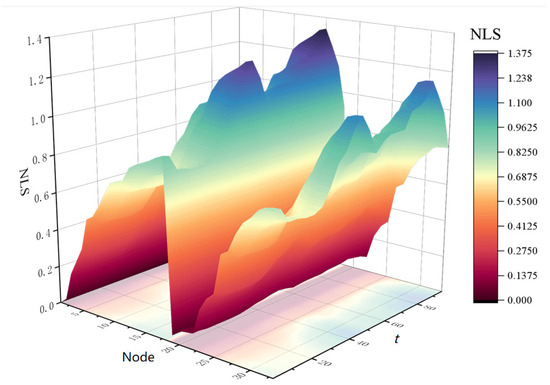
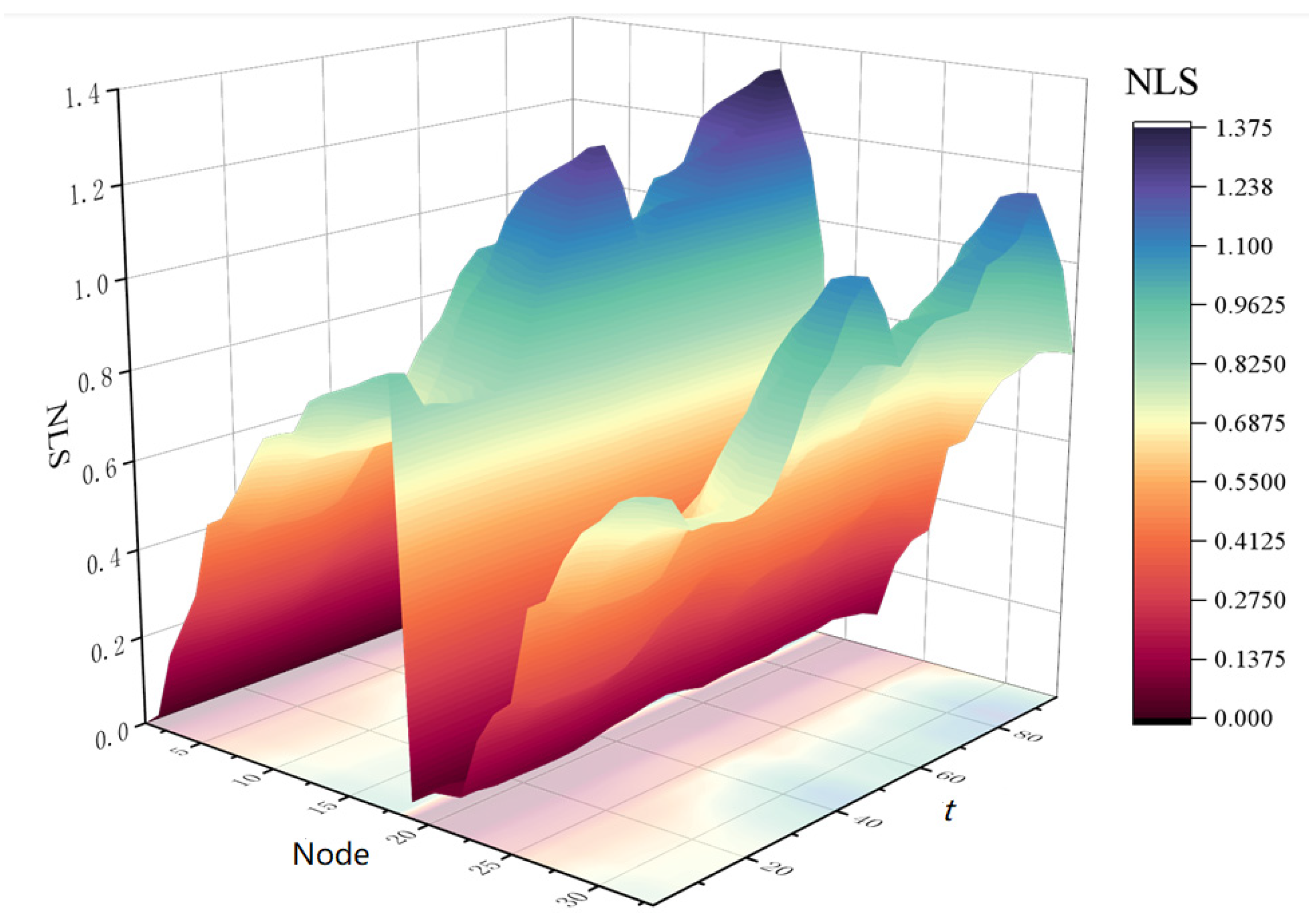
The NLS reflects the loss finger of the node after connecting the EV. Figure 11 displays the loss sensitivity of every node in the distribution network.

Figure 11. NLS for each time slot.

When Node 18 is linked to EVs, it generates the least amount of grid losses and has the lowest NLS during that time period. The node with the lowest loss performance is node 17, as shown by its greatest NLS. We often steer clear of connecting to this node when assigning EVs. Furthermore, the NLS will change throughout time. Time slot 73 is when node 17’s vulnerability to grid loss is at its highest. By combining Figure 11 and Figure 12, it is possible to determine that NLS rises as one gets further away from the balancing node 0.

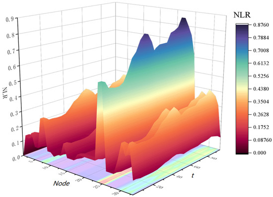
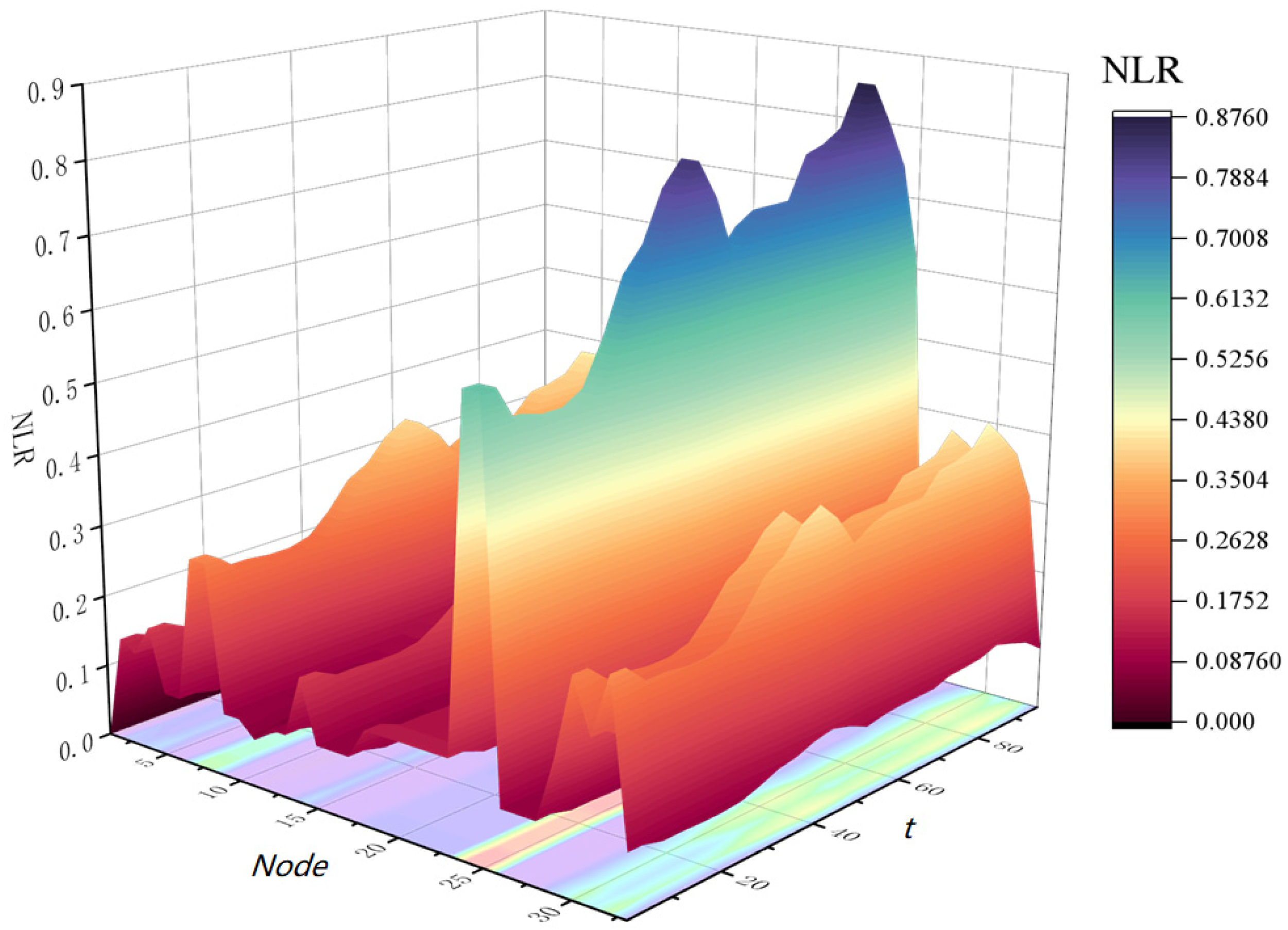
Figure 12. NLR for each time slot.

5.2.2. NLR

The Figure 12 shows the load factor of each node in every time slot, indicating that nodes 23 and 24 experience relatively high load rates as compared to the other nodes, which are subjected to lower load rates. Therefore, nodes 23 and 24 are employed to provide charging services for a limited number of EVs in order to guarantee the stability and performance of the charging system, while the other nodes are used for the charging needs of a larger number of EVs.

5.2.3. NEP

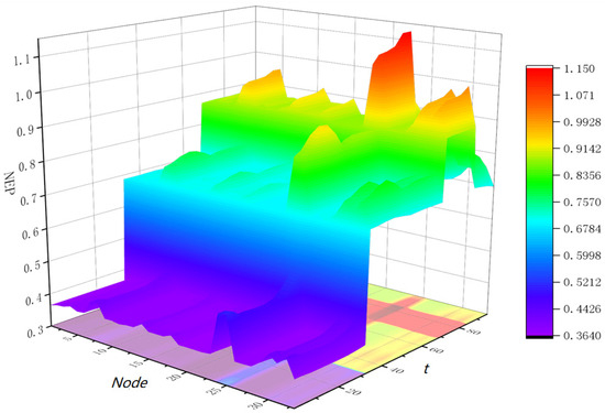
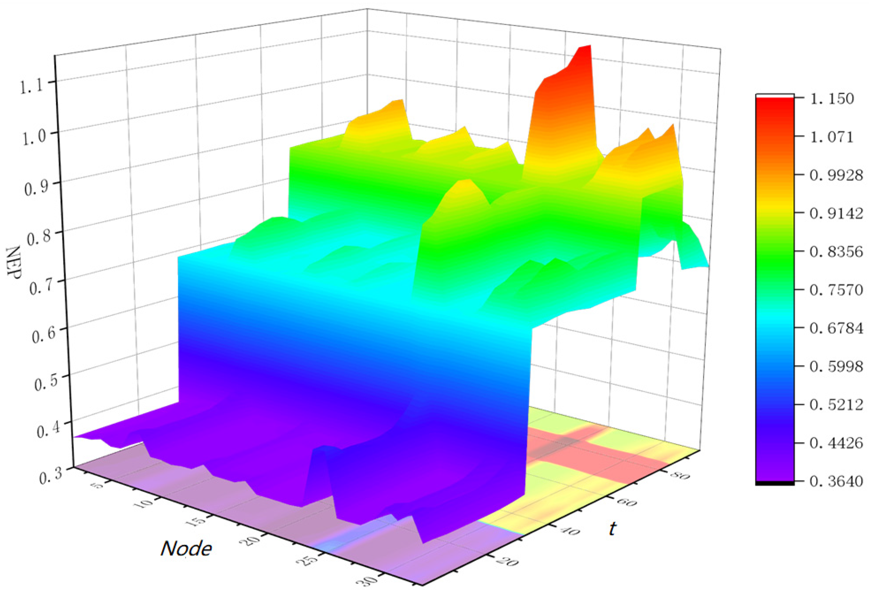
The proposed NEP is shown in Figure 13, the NEP on node 24 will be higher compared to other nodes, so the electric vehicle is charging is should be avoided to access to change the node, which will lead to increase the loss cost.

Figure 13. NEP for each time slot.

5.2.4. Electric Vehicle Charging and Discharging Results

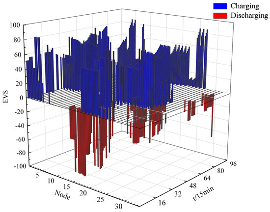
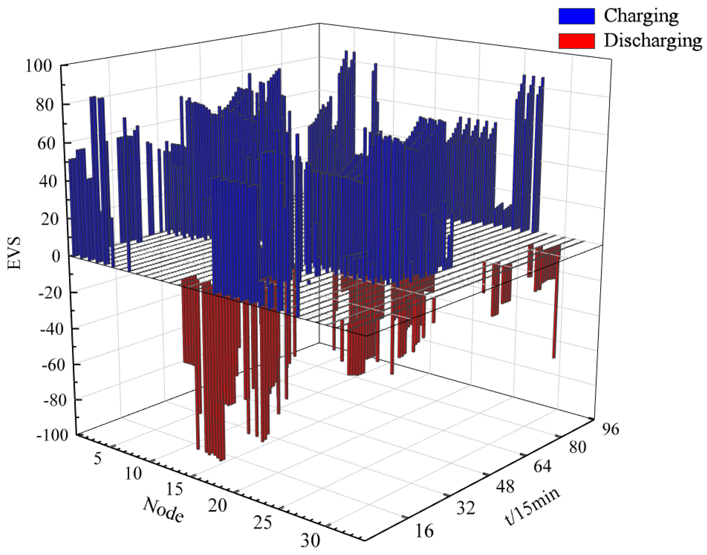
The diagram presented in Figure 14 illustrates the temporal and spatial distribution of EV charging. Nodes 1–6 and 18–26 show the highest concentration of charging and discharging activity, with smaller net export potential (NEP) and non-linear loads (NLS). This distribution aligns with the shared interests of the EVs and the grid. In the planning stage, it is advisable to construct charging stations in close proximity to the start of the distribution network. A differentiated tariff mechanism should be implemented alongside use of the elasticity coefficient method to ascertain the extent of user response. This will make it possible for EVs to be directed to charging stations close to the network’s beginning point.

Figure 14. Distribution of electric vehicle charging and discharging volumes in space and time.

To confirm that the scheduling method pro-posed in this study works as intended, three different EV access scenarios are set up to analyze EV charging costs and node loss costs. The scenarios settings are as follows

Scenario1: EVs are allocated using the plan put out in this work; Scenario2: EVs are assigned at random to every node; Scenario3: EVs are equally distributed at every node. The node loss cost (L) and EV charging cost for the various situations are shown in Table 4.

Table 4. EV charging expenses and node loss costs in different situations.

	Cost of One Node/k$	Charging Costs/k$	Total Costs/k$
Scenario 1	47.09	227.96	274.90
Scenario 2	153.31	226.34	379.65
Scenario 3	157.92	225.98	383.90

As illustrated in the Table 3, costs of charging are similar for all three scenarios, with Scenario 1 having significantly lower attrition costs than Scenarios 2 and 3. While scenario 1 overall cost is far lower, scenarios 2 and 3’s total costs are comparable. This demonstrates that lower level scheduling can effectively minimize the expenses associated with EV charging and node loss.

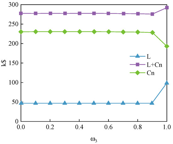
The impact of ω3 and ω4 values on node loss cost and charging cost is also examined in this paper.

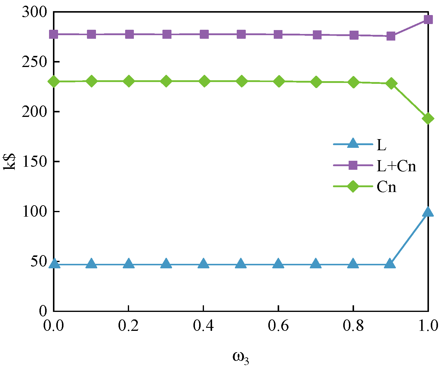
The Figure 15 illustrates how, as ω3 moves from 0 to 0.6, the overall cost of the optimal allocation virtually stays the same. It modestly declines from 0.7 to 0.9, and then increases quickly when it hits the critical number of 0.9. Thus, the overall cost of scheduling at the lower level approaches a minimum when ω3 = 0.9. In the meantime, be-cause of their coupling feature, changes in L and Cn are not readily apparent whenω3 changes from 0 to 0.9. When L = 00.00 k$, ω3 = 1. But for scenario 2 and 3, L is 158.61 k$ and 158.37 k$, respectively, which is significantly more than 100.00 k$. This demonstrates that Cn and L have a coupling property, meaning that NLS is taken into account while determining NEP.

Figure 15. Relationship between L, Cn and ω3.

6. Conclusions

This work develops an IGDT-driven sequential hierarchical scheduling scheme to coordinate bulk electric vehicle charge-discharge behavior across generation and distribution grids.

At the upper generation-side stage, an energy storage system (ESS) mathematical model is constructed. The objective function is designed to cut the operational expenditure of ESS, while optimizing the output of various power generating units and determining the optimal charge and discharge power of EV aggregations.

At the lower distribution-side stage, a nodal electricity price (NEP) framework integrated with node loss sensitivity (NLS) and node load rate (NLR) is formulated. By minimizing distribution network nodal loss expenditure together with EV charge-discharge economic costs, the scheme realizes the optimal spatial allocation of EV charging and discharging points.

Numerical simulation tests are carried out to verify the performance of the proposed framework, and the core findings are summarized as below:

The upper-layer schedule makes full use of the built wind and photovoltaic power output models. Equipped with IGDT uncertainty optimization, the upper stage can effectively cope with stochastic fluctuations of wind and solar power, boost renewable energy absorption and curtail abandoned clean energy. The simulated wind curtailment ratio reaches 0.0%, while the PV curtailment ratio is only 0.4%.

The upper hierarchical stage quantifies the ESS regulation capacity for EV flexible loads. The obtained scheduling results match the daily travel patterns of EV users, capable of satisfying the charging demand of the vast majority of electric vehicles.

Supplying EV loads purely via thermal power units (TPs) cannot guarantee energy conservation and low-carbon performance. Taking Unit TP4 as an instance, its comprehensive power generation and pollutant emission costs exceed the average charging cost of EVs in the test system.

In contrast to uniform load allocation and random EV charging arrangement modes, the NEP guidance mechanism can significantly lower nodal loss costs and overall charging expenses. Sensitivity analysis verifies that the weighting factor ω₃ = 0.9 is the optimal value to achieve the minimum total operational cost of the lower distribution network layer.

In this paper, we are assumed that the renew-able energy output does not take into account the cost nor the effect of battery loss during the dis-charge process of the EVs. However, those assumption is not realistic. In our future work, we will focus on evaluation of the cost of utilizing renewable energy to identify the best possible EVs penetration and renewable energy penetration rates. And we will examine the battery depletion in EVs charge and discharge, implement a more adaptable scheduling system, and conduct extensive research on the scheduling flexibility of EVs.

References

- Li, H.; Liu, D.; Yao, D. Analysis and reflection on the development of power system towards the goal of carbon emission peak and carbon neutrality. Proc. CSEE 2021, 41, 6245–6258. (In Chinese) [Google Scholar]
- Cheng, S.; Ni, K.; Zhao, M. Stackelberg game based bi-level coordinated optimal scheduling of microgrid accessed with charging-swapping-storage integrated station. Electr. Power Autom. Equip. 2020, 40, 49–55+69+56–59. [Google Scholar] [CrossRef]
- Va Hedipour-dahraie, M.; Rashidiza-deh-kermani, H.; Anvari-moghaddam, A.; Siano, P. Risk-averse probabilistic framework for scheduling of virtual power plants consid-ering demand response and uncertainties. Int. J. Electr. Power Energy Syst. 2020, 121, 106126. [Google Scholar] [CrossRef] [Scilit]
- Fang, F.; Yu, S.Y.; Xin, X.L. Data-driven-based stochastic robust optimization for a virtual power plant with multiple uncertainties. IEEE Trans. Power Syst. 2022, 37, 456–466. [Google Scholar] [CrossRef] [Scilit]
- Bae, S.; Kwasinski, A. Spatial and Temporal Model of Electric Vehicle Charging Demand. IEEE Trans. Smart Grid 2012, 3, 394–403. [Google Scholar] [CrossRef] [Scilit]
- Li, Z.; Yu, Q.; Gong, W.; Zhang, Z. Multi-objective Optimal Scheduling of Electricity-gas-heat Energy Hub Considering Fuzzy Chance Constraint. Proc. CSU-EPSA 2021, 33, 49–56. [Google Scholar]
- Pan, G.; Gong, M.; He, M.; Wu, C. Identification method of electricity charge recovery risk of specialized transformer user based on Stacking model fusion. Electr. Power Autom. Equip. 2021, 41, 152–160. (In Chinese) [Google Scholar]
- Peng, C.; Chen, L.; Zhang, J.; Sun, H. Multi-objective optimal allocation of energy storage in distribution network based on classified probability chance constraint information gap decision theory. Proc. CSEE 2020, 40, 2809–2818. (In Chinese) [Google Scholar] [CrossRef]
- Shojaei, A.H.; Ghadimi, A.A.; Miveh, M.R.; Gandoman, F.H.; Ahmadi, A. Multi-objective reactive power planning con-sidering the uncertainties of wind farms and loads using information gap decision theory. Renew. Energy 2021, 163, 1427–1443. [Google Scholar] [CrossRef] [Scilit]
- Cao, X.; Wang, J.; Zeng, B. A chance constrained information-gap decision model for multi-period microgrid planning. IEEE Trans. Power Syst. 2017, 33, 2684–2695. [Google Scholar] [CrossRef] [Scilit]
- Tao, Y.; Qiu, J.; Lai, S. Carbonoriented electricity network planning and transformation. IEEE Trans. Power Syst. 2021, 36, 1034–1048. [Google Scholar] [CrossRef] [Scilit]
- Yan, Q.; Lin, H.; Li, J.; Ai, X.; Shi, M.; Zhang, M.; Gejirifu, D. Many-objective charging optimization for electric vehicles considering demand response and multi-uncertainties based on Markov chain and information gap decision theory. Sustain. Cities Soc. 2022, 78, 103652. [Google Scholar] [CrossRef] [Scilit]
- Bertolini, A.; Martins, M.S.; Vieira, S.M.; Sousa, J.M. Power output optimization of electric vehicles smart charging hubs using deep rein-forcement learning. Expert Syst. Appl. 2022, 201, 116995. [Google Scholar] [CrossRef] [Scilit]
- Wang, T.; Zhang, H. Optimal charging strategy of electric vehicles based on artificial fish swarm algorithm. Electr. Mcasure-Ment. Instrum. 2023, 60, 33–38. [Google Scholar]
- Yin, W.; Ming, Z. Electric vehicle charging and discharging scheduling strategy based on local search and competitive learning particle swarm optimization algorithm. J. Energy Storage 2021, 42, 102966–102973. [Google Scholar] [CrossRef] [Scilit]
- Ling, Y.; Zhou, B.; Xu, N.; Guo, Z.; Liu, X.; Li, W.; Nie, Q.; Zhao, X. An Optimal Scheduling Method for Source-load-storage Systems Considering Carbon Trading Cost and Forecast Uncertainty. Mod. Electr. Power 2026, 43, 413–421. (In Chinese) [Google Scholar]
- Zhang, B.; Hu, W.; Cao, D.; Ghias, A.M.Y.M.; Chen, Z. Novel Data-Driven decentralized coordination model for electric vehicle aggregator and energy hub entities in mul-ti-energy system using an improved multi-agent DRLapproach. Appl. Energy 2023, 339, 120902. [Google Scholar] [CrossRef] [Scilit]
- Qiu, D.; Yang, H.; Lai, M. Optimal bidding strategy and EV charging management of intelligent regional aggre- gators based on CVaR method. Syst. Eng.-Theory Pract. 2018, 38, 1994–2005. [Google Scholar]
- Wang, Y.; Ma, X.; Wan, Y.; Hou, X.; Zheng, K.; Chen, W. Sequential Charge-discharge Guidance Strategy for Elec-tric Vehicles Based on Time-sharing Charging-discharging Margin. Power Syst. Technol. 2019, 43, 4353–4361. (In Chinese) [Google Scholar]
- Hou, H.; Wang, Y.; Zhao, B.; Zhang, L.; Chen, Y.; Xie, C. Electric Vehicle Aggregator Dispatching Strategy Un-der Price and Incentive Demand Response. Power Syst. Technol. 2022, 46, 1259–1269. (In Chinese) [Google Scholar]
- Cui, J.; Luo, W.; Zhou, N. Research on Pricing Model and Strat-egy of Electric Vehicle Charging and Dis-charging Based on Multi View. Proc. CSEE 2018, 38, 4438–4450+4644. (In Chinese) [Google Scholar]
- Pan, Z.; Yu, T.; Wang, K. Decentralized Coordinated Dispatch for Real-time Optimization of Massive Electric Ve- hicles Considering Various Interest. Proc. CSEE 2019, 39, 3528–3541. (In Chinese) [Google Scholar]
- Wei, W.E.I.; Chen, Y.; Liu, F.; Mei, S.W.; Tian, F.; Zhang, X. Stackelberg Game Based Retailer Pricing Scheme and EV Charging Management in Smart Residential Area. Power Syst. Technol. 2015, 39, 939–945. [Google Scholar]
- Loaiza Quintana, C.; Climent, L.; Arbelaez, A. A Robust Optimization Framework for eBus Charging Infrastructure Planning. J. Heuristics 2026, 32, 12. [Google Scholar] [CrossRef] [Scilit]
- Saber, A.Y.; Ve-nayagamoorthy, G.K. Resource Scheduling Under Uncertainty in a Smart Grid with Renewables and Plug-in Vehicles. IEEE Syst. J. 2012, 6, 103–109. [Google Scholar] [CrossRef] [Scilit]
Disclaimer/Publisher’s Note: The statements, opinions and data contained in all publications are solely those of the individual author(s) and contributor(s) and not of MDPI and/or the editor(s). MDPI and/or the editor(s) disclaim responsibility for any injury to people or property resulting from any ideas, methods, instructions or products referred to in the content. |
© 2026 by the authors. Licensee MDPI, Basel, Switzerland. This article is an open access article distributed under the terms and conditions of the Creative Commons Attribution (CC BY) license.