Segmented Finite Line Source Analysis of Mid-Deep UBHE with Geothermal Gradient and Stratification

Abstract

This study develops an analytical model for a mid-deep U-shaped borehole heat exchanger (UBHE) based on the segmented finite line source method, integrating geothermal gradient, five-layer geological stratification, and groundwater seepage within a unified framework. The injection, horizontal, and extraction sections are represented by independent local coordinates and coupled through the position- and time-dependent unit-length heat-transfer rate $q_l\left(s_n,t\right)$. Validation against the benchmark results of Bao et al. yields a mean absolute error of 0.87 °C and a mean relative error of 1.6%. Numerical-independence tests identify a 1 h time step and 100/50 m vertical/horizontal segment lengths as the adopted settings, and the iterative residual reaches 10⁻⁴ °C within eight iterations for the representative case. In a homogeneous, no-seepage limiting case, the model agrees with the classical finite line-source solution with an MAE of 0.012 °C and a maximum relative-error magnitude of 0.41%. The extraction-well fluid-temperature peak occurs at 600–800 m depth, whereas the local heat-transfer direction changes near 1600 m. For the investigated 2500–650–2500 m geometry, the highest cycle-averaged outlet temperature is obtained at an insulation length of 1600 m. Sensitivity analyses further quantify the effects of seepage velocity, equivalent thermal conductivity, geothermal gradient, and the validation insulation-length assumption.

1. Introduction

The global dependence on non-renewable energy sources presents substantial challenges to environmental sustainability and energy security. Therefore, transitioning to renewable energy is critical to mitigating fossil fuel reliance [1,2,3]. Among renewable resources, geothermal energy stands out as a promising alternative due to its vast reserves, low environmental impact, and stable performance, unaffected by climatic fluctuations. It is increasingly utilized for both power generation and space heating and cooling applications [4,5,6].

Geothermal heat pump technology, which employs borehole heat exchangers (BHEs) for subsurface heat transfer, is a primary application of geothermal energy [7]. Shallow systems typically utilize boreholes with depths under 200 m [8,9]. However, their low heat exchange capacity per unit length [10] requires a high density of boreholes to meet large-scale thermal demands, making the technology land-intensive. Additionally, seasonal load imbalances in certain regions can lead to long-term soil thermal degradation [11]. To address these limitations, mid-deep borehole heat exchangers (DBHEs) are increasingly adopted due to their higher thermal recovery capacity and more consistent performance.

DBHE systems typically extract geothermal energy at depths between 1500 and 3000 m [12]. The main configurations include coaxial borehole heat exchangers (CBHEs) and deep butted well systems. The CBHE [13] consists of an inner pipe and an outer casing, with fluid circulating between the annulus and the inner pipe. In contrast, the deep butted well system comprises an injection well, a horizontal section, and an extraction well. The horizontal section increases the thermal contact area with deep formations, which improves the heat extraction performance.

Research on DBHEs mainly relies on numerical simulations [14,15], focusing on model development and verification [16,17,18,19], parametric sensitivity analysis [20,21,22,23], thermal influence radius determination [24,25], and temperature recovery mechanisms [26]. Additionally, the heat capacity of CBHEs can be predicted using the thermophysical properties of the formation and fluid [27]. However, while numerical models provide high accuracy in simulating complex heat transfer processes [28,29], they require high computational costs and long simulation times, particularly for long-term performance evaluations.

Analytical models provide an alternative to numerical methods for predicting BHE thermal performance. Although these models rely on simplifying assumptions, they effectively characterize heat extraction mechanisms and primary heat transfer processes when fundamental physical constraints are properly defined.

Borehole heat exchangers (BHEs) are typically modeled as line or cylindrical heat sources within finite or infinite media, assuming uniform thermophysical properties [30,31]. Most existing models emphasize radial conduction while neglecting axial effects, making them primarily suitable for short-term predictions. However, accurate long-term performance evaluations necessitate model adjustments to incorporate the cumulative thermal impacts and axial heat flow.

Existing finite line source (FLS) models [30,31] account for conduction and axial effects but often neglect groundwater seepage. Seepage introduces a coupled conduction–convection mechanism [32,33], which reduces thermal accumulation near the borehole. Studies have shown that groundwater flow enhances the heat transfer performance between the heat exchanger and the aquifer [34,35,36].

Studies on DBHEs underground water seepage primarily focus on CBHE configurations. The convolution theorem was applied to determine borehole wall temperatures [37], while semi-analytical models were developed to account for geothermal gradients and heat capacity changes [38]. Using the Moving Finite Line Source (MFLS) method, Jiao et al. [21,26] investigated horizontal seepage and formation temperature recovery. Luo et al. [39,40,41,42] introduced segmented FLS and FCS models to characterize geothermal gradients, fluid heat transfer, and stratified geological layers. Their findings indicated that higher geothermal gradients increase extraction efficiency and that annular-inflow configurations achieve better performance than annular-outflow modes [39].

Analytical solutions have been used to optimize heat extraction and characterize thermal recovery [43,44]. Huang et al. [20] developed a framework considering ground heterogeneity. Jia et al. [45] established a semi-analytical model for a horizontally butted borehole system with groundwater seepage and geothermal gradient, whereas Luo et al. [39,40,41] focused on deep coaxial configurations and segmented responses in layered formations. These studies provide important foundations but do not describe the same three-segment UBHE geometry, segment-wise fluid equations, and insulation optimization considered here.

Mathematical modeling of mid-deep borehole heat exchangers (DBHEs) under complex conditions, such as groundwater seepage and geological stratification, remains limited. Developing analytical frameworks that incorporate realistic geological features is essential for advancing this field. Most existing finite line source (FLS) models assume uniform heat flux and neglect geological heterogeneity and geothermal gradients. Although Jia et al. [45] addressed seepage in butted-well systems, a unified symmetric UBHE framework that simultaneously incorporates equivalent porous-media seepage, five-layer stratification, and long-term cyclic insulation optimization has not been reported. Given the substantial depth and multi-layered environment of DBHEs, these factors must be integrated into heat transfer models to ensure accuracy.

This study develops an analytical model for a mid-deep U-shaped borehole heat exchanger that integrates geothermal gradient, formation stratification, groundwater seepage, and extraction-well insulation. The methodological contribution is a unified and extensible coupling framework rather than a claim of a new fundamental heat-transfer mechanism. Specifically, the injection, horizontal, and extraction sections are assigned independent local coordinates; the formation response retains the superposed contributions of all finite line-source segments; and the one-dimensional fluid equations are coupled to the formation through $q_l\left(s_n,t\right)$. Layer-specific equivalent porous-medium properties enter the segment response directly. The model is evaluated through benchmark comparison, numerical-independence tests, analytical limiting-case verification, and parameter-sensitivity analyses. A direct comparison with the relevant models is provided in Section 4.4.4.

2. Model Building

2.1. Physical Model

2.1.1. The System Composition and Principles

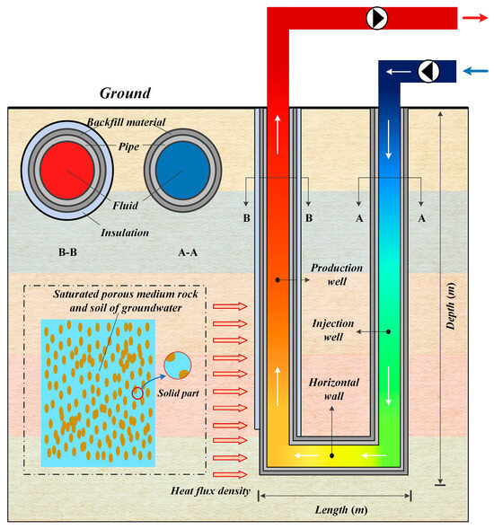
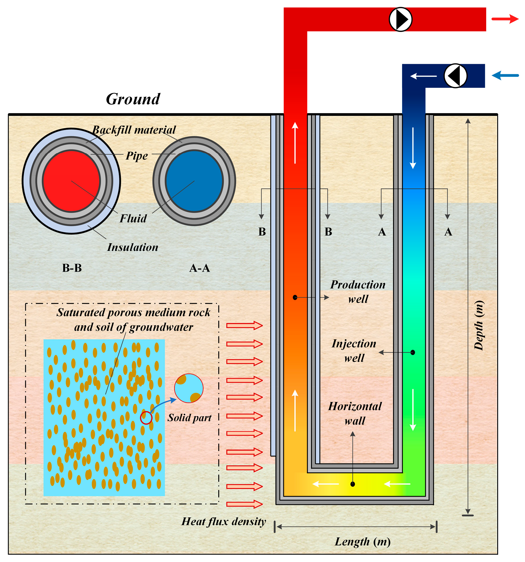
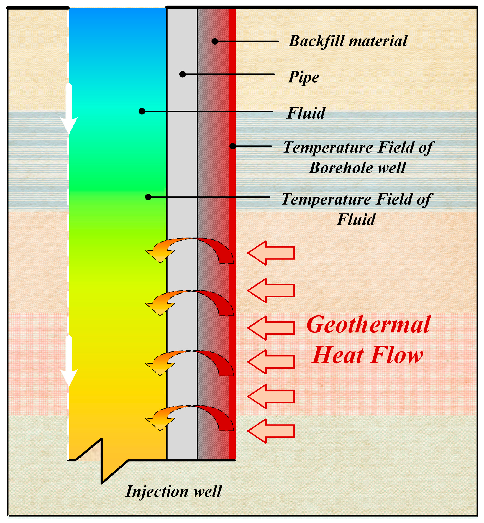
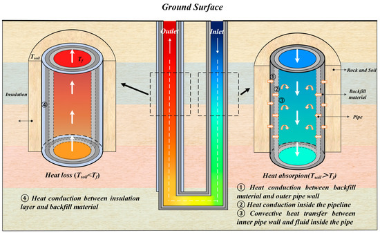
Figure 1 illustrates the UBHE configuration, consisting of injection, horizontal, and extraction segments. The fluid, pipeline, and backfill are thermally coupled to the formation. The closed-loop cycle involves downward injection, horizontal heat extraction, and upward recovery. Insulation in the extraction well minimizes reverse heat exchange with shallow strata.

Figure 1. Composition and working principles of the UBHE system. Reproduced from Ref. [46] under the Creative Commons Attribution (CC BY 4.0) license.

The one-dimensional fluid equations are solved separately along the injection, horizontal, and extraction flow-path segments. In contrast, the formation-temperature response retains the superposed thermal contributions of all three line-source segments. Direct thermal short-circuiting through the borehole structure and long-range inter-well interference are neglected, but cross-segment formation responses are not removed from the temperature-field solution.

2.1.2. Modeling Framework and Assumptions

The development of the proposed model is governed by the following core logic:

(i)

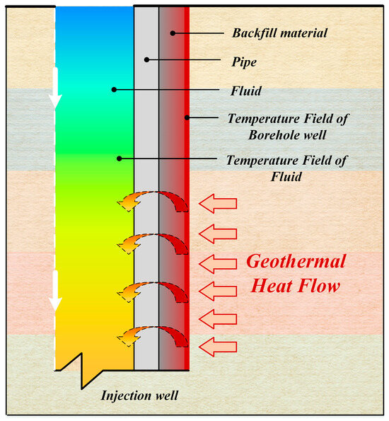
Thermal Boundary Identification: The borehole wall serves as the primary interface for heat exchange between the subsurface formation and the circulating fluid. As shown in Figure 2, all heat flux from the surrounding formation must penetrate this boundary to interact with the fluid within the pipes.

Figure 2. Core ideas of modeling. Reproduced from Ref. [46] under the Creative Commons Attribution (CC BY 4.0) license.

(ii)

Coupling Mechanism: Following Li et al. [47], the unit-length heat-transfer rate q_l is utilized as the coupling parameter. By representing the instantaneous heat flow from the formation to the borehole, q_l links the governing equations of the ground temperature field with the fluid thermal dynamics, enabling a rigorous mathematical formulation.

(iii)

Numerical Implementation: The model is implemented using a custom iterative algorithm in MATLAB R2023b. In this scheme, the q_l output from each time step updates the temperature distribution for the subsequent cycle. This computational workflow determines the evolution of the outlet fluid temperature and the total heat extraction capacity.

The following assumptions are adopted to simplify the model while maintaining the primary heat transfer mechanisms:

(i)

Formation Representation: Each geological layer is treated as a homogeneous and isotropic porous medium saturated with groundwater, while thermophysical properties vary between layers. The formation response includes radial and axial conduction. Layer interfaces are represented through a layer-wise equivalent approximation in which each integration element uses the properties of the stratum containing that element; the model does not explicitly resolve local interfacial temperature and heat-flux fields.

(ii)

Fluid Dynamics: The working fluid is incompressible, and its velocity and temperature are cross-sectionally averaged. The one-dimensional approximation is appropriate for the high-aspect-ratio pipes considered here, but it does not resolve cross-sectional temperature gradients or local U-bend effects.

(iii)

Thermophysical Properties: The properties of each geological layer, the pipe, the backfill, the insulation, and the working fluid are treated as temperature-independent constants. The general Green-function derivation permits anisotropy, whereas all calculations in this study use the isotropic special case $k_x=k_y=k_z=k_{\mathrm{e}\mathrm{q}\mathrm{u},j}$ within each layer.

Justification and Impact of Assumptions: The one-dimensional fluid treatment and layer-wise constant properties provide a computationally efficient analytical framework for system-level and long-term parametric analysis. Neglecting contact resistance may overestimate heat transfer, and the constant-property approximation is less appropriate for large temperature-dependent property variations or strongly heterogeneous layers. Neglecting the local U-bend geometry primarily affects the bottom-hole neighborhood, while neglecting inter-well interference is restricted to configurations in which the well spacing remains much larger than the thermal influence radius. No unsupported universal error percentage is assigned to these approximations.

2.1.3. Surface Boundary Verification and Inter-Well Thermal Interference

Two auxiliary quantities are used to state the surface-boundary and inter-well assumptions. $\Delta T_{\mathrm{s}\mathrm{u}\mathrm{r}\mathrm{f}}$ denotes the temperature perturbation relative to the undisturbed geothermal field at $z=0$. $R_{\mathrm{t}\mathrm{h}}$ is the thermal influence radius, estimated as $R_{\mathrm{t}\mathrm{h}}\approx 2\sqrt{\alpha t}$ using the representative formation diffusivity and operating time.

An opposite-sign image line source cancels the temperature perturbation produced by the real source at $z=0$ and therefore satisfies a constant-temperature Dirichlet boundary condition. A same-sign image source would instead represent a zero-normal-heat-flux Neumann condition. The present model uses the opposite-sign image source consistently in the main equations and Appendix A.

For the benchmark geometry, the horizontal separation is 684 m. At $t=8760\hspace{0.17em}\mathrm{h}$ and $\alpha \approx 1.0\times {10}^{-6}\hspace{0.17em}{\mathrm{m}}^2/\mathrm{s}$, $R_{\mathrm{t}\mathrm{h}}\approx 4.5\hspace{0.17em}\mathrm{m}$, giving $L_w/R_{\mathrm{t}\mathrm{h}}\approx 150$. Thus, long-range inter-well interference is neglected for the present geometry. This assumption is not generalized to closely spaced multi-borehole fields and is stated as a model limitation.

2.2. Mathematical Model

This section formulates the UBHE thermal response using conventional notation and established heat-source solutions from earlier UBHE studies [32,46,47,48].

2.2.1. Derivation of the Segmented FLS Model

(1)

The segmented FLS formulation is developed through the steps below, while Appendix A provides the full derivation. The procedure extends the analytical framework reported in Ref. [46].

The derivation begins with the Green’s function for a unit instantaneous point source acting at time t′ and coordinates X′ = (x′, y′, z′) [48]:

$$\mathrm{G}(\mathrm{X},\mathrm{t};{\mathrm{X}}^{\prime },{\mathrm{t}}^{\prime })={\displaystyle \frac{[\mathsf{\rho }\mathrm{c}/(\mathrm{t}-{\mathrm{t}}^{\prime }){]}^{3/2}}{8{\mathsf{\pi }}^{3/2}\sqrt{{\mathrm{k}}_{\mathrm{x}}{\mathrm{k}}_{\mathrm{y}}{\mathrm{k}}_{\mathrm{z}}}}}\exp \{-{\displaystyle \frac{\mathsf{\rho }\mathrm{c}}{4(\mathrm{t}-{\mathrm{t}}^{\prime })}}[{\displaystyle \frac{(\mathrm{x}-{\mathrm{x}}^{\prime }{)}^2}{{\mathrm{k}}_{\mathrm{x}}}}+{\displaystyle \frac{(\mathrm{y}-{\mathrm{y}}^{\prime }{)}^2}{{\mathrm{k}}_{\mathrm{y}}}}+{\displaystyle \frac{(\mathrm{z}-{\mathrm{z}}^{\prime }{)}^2}{{\mathrm{k}}_{\mathrm{z}}}}]\}$$

(1)

Here, X = (x, y, z) denotes the observation point. The parameters kx, ky, and kz are the directional thermal conductivities, expressed in W/(m·K).

For continuous source operation from t′ = 0 to t′ = t, integration over release time gives the point-source temperature response θp(X,t):

$${\mathsf{\theta }}_{\mathrm{p}}(\mathrm{X},\mathrm{t})={\displaystyle \frac{(\mathsf{\rho }\mathrm{c}/\mathsf{\pi }{)}^{3/2}}{8\sqrt{{\mathrm{k}}_{\mathrm{x}}{\mathrm{k}}_{\mathrm{y}}{\mathrm{k}}_{\mathrm{z}}}}}{\int }_0^{\mathrm{t}}{\displaystyle \frac{1}{(\mathrm{t}-{\mathrm{t}}^{\prime }{)}^{3/2}}}\exp \{-{\displaystyle \frac{\mathsf{\rho }\mathrm{c}}{4(\mathrm{t}-{\mathrm{t}}^{\prime })}}[{\displaystyle \frac{(\mathrm{x}-{\mathrm{x}}^{\prime }{)}^2}{{\mathrm{k}}_{\mathrm{x}}}}+{\displaystyle \frac{(\mathrm{y}-{\mathrm{y}}^{\prime }{)}^2}{{\mathrm{k}}_{\mathrm{y}}}}+{\displaystyle \frac{(\mathrm{z}-{\mathrm{z}}^{\prime }{)}^2}{{\mathrm{k}}_{\mathrm{z}}}}]\}\mathrm{d}{\mathrm{t}}^{\prime }$$

(2)

Introducing the following auxiliary parameters simplifies the time integral and gives Equation (3):

$${\kappa }_{zx}={\displaystyle \frac{k_z}{k_x}}, {\kappa }_{zy}={\displaystyle \frac{k_z}{k_y}}, {\tau }^{-2}=t-t^{\prime }, d={\left[{\kappa }_{zx}{\left(x-x^{\prime }\right)}^2+{\kappa }_{zy}{\left(y-y^{\prime }\right)}^2+{\left(z-z^{\prime }\right)}^2\right]}^{1/2}$$

$${\mathsf{\theta }}_{\mathrm{p}}(\mathrm{X},\mathrm{t})={\displaystyle \frac{(\mathsf{\rho }\mathrm{c}/\mathsf{\pi }{)}^{3/2}}{4\sqrt{{\mathrm{k}}_{\mathrm{x}}{\mathrm{k}}_{\mathrm{y}}{\mathrm{k}}_{\mathrm{z}}}}}{\int }_{1/\sqrt{\mathrm{t}}}^{\infty }\exp (-{\displaystyle \frac{{\mathrm{d}}^2{\mathsf{\tau }}^2}{4{\mathsf{\alpha }}_{\mathrm{z}}}})\mathrm{d}\mathsf{\tau }={\displaystyle \frac{1}{4\mathsf{\pi }\mathrm{d}\sqrt{{\mathsf{\alpha }}_{\mathrm{x}}{\mathsf{\alpha }}_{\mathrm{y}}}}}\mathrm{erfc}({\displaystyle \frac{\mathrm{d}}{2\sqrt{{\mathsf{\alpha }}_{\mathrm{z}}\mathrm{t}}}})$$

(3)

The quantities αx, αy, and αz are the directional thermal diffusivities (m²/s). The remaining time integral is evaluated using the complementary error function.

The finite line-source response is obtained by distributing the point source continuously along a vertical segment of length L [46,47]. The segment extends downward from z = 0 in a semi-infinite anisotropic medium and releases heat at a prescribed rate per unit length. Its temperature response follows by integrating over the source coordinate X′ = (x′, y′, z′).

Spatial integration of Equation (3) along the source segment produces the temperature-response expression in Equation (4):

$$\mathsf{\theta }(\mathrm{z},\mathrm{t})={\displaystyle \frac{{\mathrm{q}}_{\mathrm{l}}}{4\mathsf{\pi }\sqrt{{\mathrm{k}}_{\mathrm{x}}{\mathrm{k}}_{\mathrm{y}}}}}{\int }_0^{\mathrm{L}}{\displaystyle \frac{1}{\mathrm{d}}}\mathrm{erfc}({\displaystyle \frac{\mathrm{d}}{2\sqrt{{\mathsf{\alpha }}_{\mathrm{z}}\mathrm{t}}}})\mathrm{d}{\mathrm{z}}^{\prime }$$

(4)

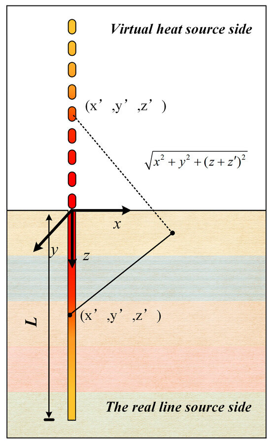
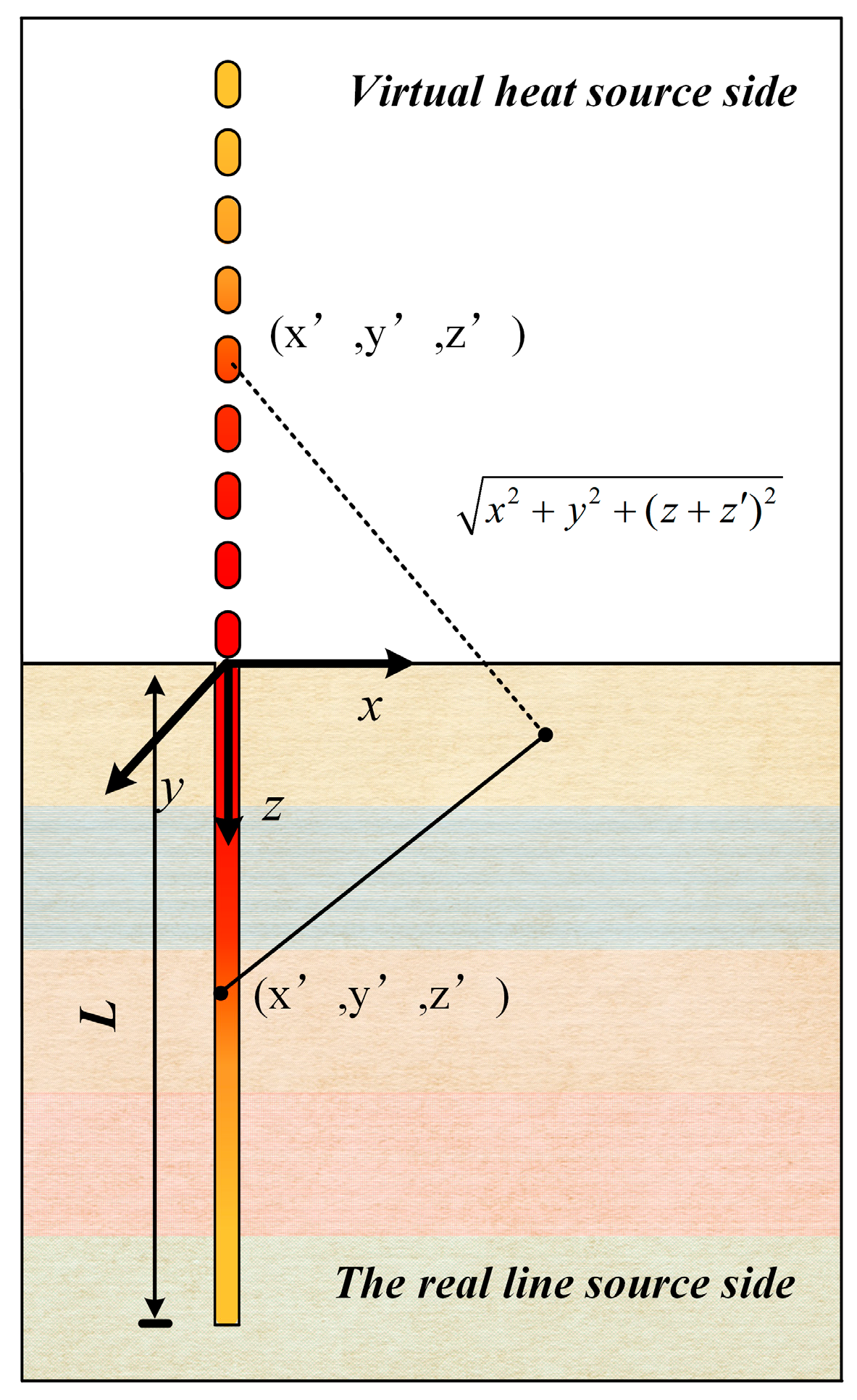
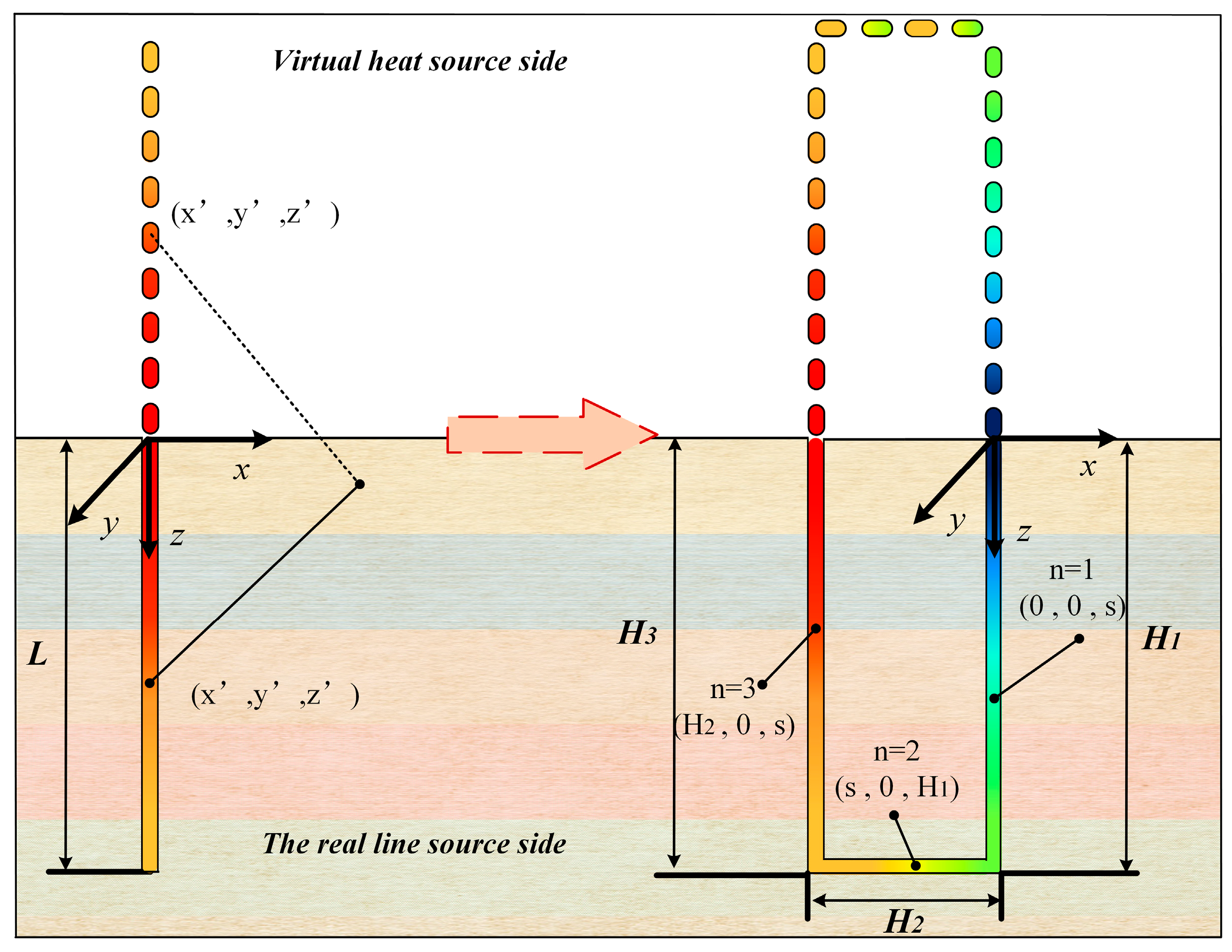
The virtual image method is introduced to satisfy the prescribed constant-temperature boundary at the ground surface of the semi-infinite domain. The image line source has the opposite sign to the real source, so their temperature perturbations cancel at $z=0$. The virtual heat-source configuration is shown in Figure 3.

Figure 3. Schematic diagram of the virtual heat source method. Reproduced from Ref. [46] under the Creative Commons Attribution (CC BY 4.0) license.

The reflected source contributes the temperature-response term given in Equation (5):

$${\mathsf{\theta }}^{\prime }(\mathrm{z},\mathrm{t})=-{\displaystyle \frac{{\mathrm{q}}_{\mathrm{l}}}{4\mathsf{\pi }\sqrt{{\mathrm{k}}_{\mathrm{x}}{\mathrm{k}}_{\mathrm{y}}}}}{\int }_0^{\mathrm{L}}{\displaystyle \frac{1}{{\mathrm{d}}^{\prime }}}\mathrm{erfc}({\displaystyle \frac{{\mathrm{d}}^{\prime }}{2\sqrt{{\mathsf{\alpha }}_{\mathrm{z}}\mathrm{t}}}})\mathrm{d}{\mathrm{z}}^{\prime }$$

(5)

Among them, ${\mathrm{d}}^{\prime }=\sqrt{{\mathsf{\kappa }}_{\mathrm{z}\mathrm{x}}(\mathrm{x}-{\mathrm{x}}^{\prime }{)}^2+{\mathsf{\kappa }}_{\mathrm{z}\mathrm{y}}(\mathrm{y}-{\mathrm{y}}^{\prime }{)}^2+(\mathrm{z}+{\mathrm{z}}^{\prime }{)}^2}$.

Superposing the real-source and reflected-source contributions yields the FLS temperature response in Equation (6):

$${\mathsf{\theta }}_{\mathrm{fls}}(\mathrm{z},\mathrm{t})=\mathsf{\theta }+{\mathsf{\theta }}^{\prime }={\displaystyle \frac{{\mathrm{q}}_{\mathrm{l}}}{4\mathsf{\pi }\sqrt{{\mathrm{k}}_{\mathrm{x}}{\mathrm{k}}_{\mathrm{y}}}}}{\int }_0^{\mathrm{L}}[{\displaystyle \frac{\mathrm{erfc}(\mathrm{d}/2\sqrt{{\mathsf{\alpha }}_{\mathrm{z}}\mathrm{t}})}{\mathrm{d}}}-{\displaystyle \frac{\mathrm{erfc}({\mathrm{d}}^{\prime }/2\sqrt{{\mathsf{\alpha }}_{\mathrm{z}}\mathrm{t})}}{{\mathrm{d}}^{\prime }}}]\mathrm{d}{\mathrm{z}}^{\prime }$$

(6)

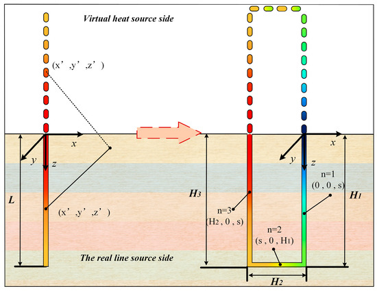
Equation (6) is extended to the three UBHE segments. Independent local coordinates $s_1$, $s_2$, and $s_3$ are used for the injection, horizontal, and extraction sections, respectively, so that the integration interval of each segment is defined by its own physical length.

The local coordinates and global source-point coordinates are defined as follows:

$$n=1: s_1\in \left[0,H_1\right], {{\mathbf{X}}^{\prime }}_1=\left(0,0,s_1\right), z_1\left(s_1\right)=s_1$$

$$n=2: s_2\in \left[0,L_h\right], {{\mathbf{X}}^{\prime }}_2=\left(s_2,0,H_1\right), z_2\left(s_2\right)=H_1$$

$$n=3: s_3\in \left[0,H_3\right], {{\mathbf{X}}^{\prime }}_3=\left(L_h,0,H_1-s_3\right), z_3\left(s_3\right)=H_1-s_3$$

The corresponding real-source and image-source distances are defined with squared coordinate differences:

$$d_1={\left[{\kappa }_{zx}{x}^2+{\kappa }_{zy}{y}^2+{\left(z-s_1\right)}^2\right]}^{1/2}; {d^{\prime }}_1={\left[{\kappa }_{zx}{x}^2+{\kappa }_{zy}{y}^2+{\left(z+s_1\right)}^2\right]}^{1/2}$$

$$d_2={\left[{\kappa }_{zx}{\left(x-s_2\right)}^2+{\kappa }_{zy}{y}^2+{\left(z-H_1\right)}^2\right]}^{1/2}; {d^{\prime }}_2={\left[{\kappa }_{zx}{\left(x-s_2\right)}^2+{\kappa }_{zy}{y}^2+{\left(z+H_1\right)}^2\right]}^{1/2}$$

$$d_3={\left[{\kappa }_{zx}{\left(x-L_h\right)}^2+{\kappa }_{zy}{y}^2+{\left(z-H_1+s_3\right)}^2\right]}^{1/2}; {d^{\prime }}_3={\left[{\kappa }_{zx}{\left(x-L_h\right)}^2+{\kappa }_{zy}{y}^2+{\left(z+H_1-s_3\right)}^2\right]}^{1/2}$$

Here, $H_1$ and $H_3$ denote the vertical lengths of the injection and extraction wells, respectively, and $L_h$ denotes the horizontal-section length. The vertical-depth functions are $z_1\left(s_1\right)=s_1$, $z_2\left(s_2\right)=H_1$, and $z_3\left(s_3\right)=H_1-s_3$.

Substitution of the three local-coordinate definitions into Equation (6) gives the segmented FLS superposition used to calculate the borehole-wall temperature:

$$T_b\left(\mathbf{X},t\right)={\displaystyle \sum _{n=1}^3}{\displaystyle \frac{q_l\left(s_n,t\right)}{4\pi \sqrt{k_{x,n}{k}_{y,n}}}}{\int }_0^{L_n}\left[{\displaystyle \frac{\mathrm{e}\mathrm{r}\mathrm{f}\mathrm{c}\left(d_n/\left(2\sqrt{{\alpha }_{z,n}t}\right)\right)}{d_n}}-{\displaystyle \frac{\mathrm{e}\mathrm{r}\mathrm{f}\mathrm{c}\left({d^{\prime }}_n/\left(2\sqrt{{\alpha }_{z,n}t}\right)\right)}{{d^{\prime }}_n}}\right]d{s}_n$$

(7)

In Equation (7), $L_1=H_1$, $L_2=L_h$, and $L_3=H_3$. The quantity $q_l\left(s_n,t\right)$ is allowed to vary with segment position and time, and the formation response includes the contributions of all three segments. The extended virtual heat-source configuration is shown in Figure 4.

Figure 4. Schematic diagram of the extended virtual heat source method. Reproduced from Ref. [46] under the Creative Commons Attribution (CC BY 4.0) license.

The unit-length heat-transfer rate between the borehole wall and the fluid is defined as:

$$q_l\left(s,t\right)={\displaystyle \frac{T_b\left(s,t\right)-T_f\left(s,t\right)}{R^{\prime }}}$$

(8)

$R\prime$ is the total thermal resistance per unit length, with units of m·K/W. Therefore, no additional segment length is included in Equation (8). The sign convention is $q_l>0$ for heat transferred from the formation to the fluid and $q_l<0$ for heat lost from the fluid to the formation.

(2)

Groundwater seepage is incorporated through the following equivalent formation properties:

Following the equivalent porous-medium approximation, the layer thermal conductivity and volumetric heat capacity are evaluated using Equations (9) and (10):

$${\mathrm{k}}_{\mathrm{equ}}={\mathrm{k}}_{\mathrm{s}}+{\mathsf{\rho }}_{\mathrm{f}}{\mathrm{c}}_{\mathrm{f}}{\mathrm{v}}_{\mathrm{f}}{\mathrm{L}}_{\mathrm{c}}$$

(9)

$${\mathsf{\rho }}_{\mathrm{equ}}{\mathrm{c}}_{\mathrm{equ}}=\mathsf{\phi }{\mathsf{\rho }}_{\mathrm{f}}{\mathrm{c}}_{\mathrm{f}}+(1-\mathsf{\phi }){\mathsf{\rho }}_{\mathrm{s}}{\mathrm{c}}_{\mathrm{s}}$$

(10)

Here, ${\rho }_{\mathrm{e}\mathrm{q}\mathrm{u}}{c}_{\mathrm{e}\mathrm{q}\mathrm{u}}$ is the equivalent volumetric heat capacity; $k_s$ is the solid-matrix thermal conductivity; $v_f$ is the seepage velocity; φ is porosity; and the characteristic length is fixed at $L_c=10\hspace{0.17em}\mathrm{m}$ in all calculations. The seepage sensitivity analysis varies $v_f$ from 0 to three times its baseline value while retaining $L_c=10\hspace{0.17em}\mathrm{m}$; conclusions are restricted to this investigated range.

2.2.2. The Temperature Field of Borehole Walls

(1)

The following relation describes the energy balance of the circulating fluid:

Using the cross-sectional area $A_f$, mean velocity $u_f$, and volumetric flow rate $\dot{V}=A_f{u}_f$, the dimensionally consistent one-dimensional fluid energy equation is:

$${\rho }_f{c}_f{A}_f{\displaystyle \frac{\partial T_f\left(s,t\right)}{\partial t}}+{\rho }_f{c}_f\dot{V}{\displaystyle \frac{\partial T_f\left(s,t\right)}{\partial s}}=q_l\left(s,t\right)$$

(11)

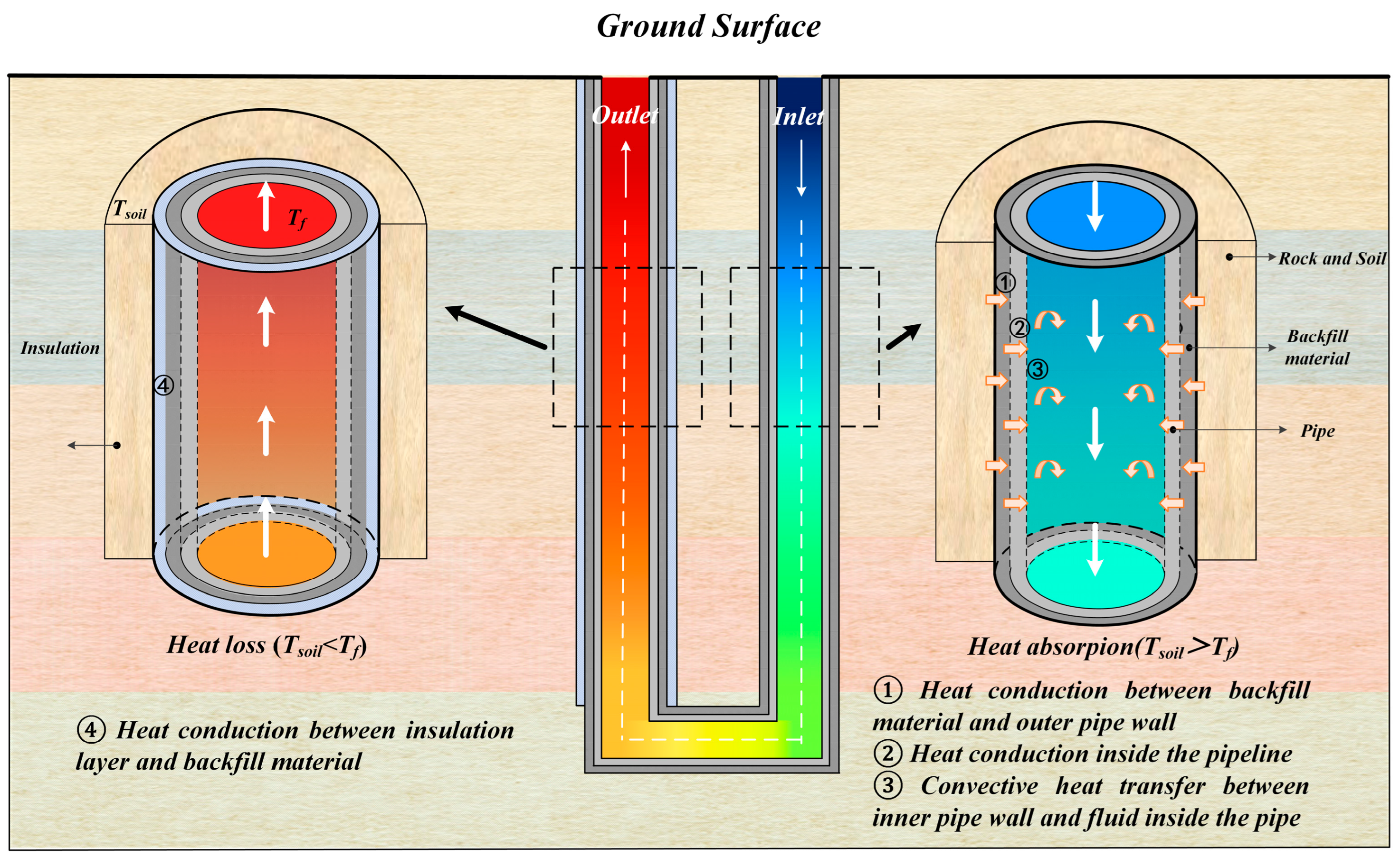
Figure 5 separates the total system resistance into four components. Labels ①–④ denote Re, Rm, Ri, and RI, respectively:

Figure 5. Schematic illustration of the heat-exchange principle. Reproduced from Ref. [46] under the Creative Commons Attribution (CC BY 4.0) license.

Equation (12) defines the total thermal resistance and its individual components:

$$R\prime =R{\prime }_{\mathrm{c}\mathrm{o}\mathrm{n}\mathrm{v}}+{R^{\prime }}_{\mathrm{p}\mathrm{i}\mathrm{p}\mathrm{e}}+{R^{\prime }}_{\mathrm{b}\mathrm{a}\mathrm{c}\mathrm{k}\mathrm{f}\mathrm{i}\mathrm{l}\mathrm{l}}+{R^{\prime }}_I$$

(12)

$$R{\prime }_{\mathrm{b}\mathrm{a}\mathrm{c}\mathrm{k}\mathrm{f}\mathrm{i}\mathrm{l}\mathrm{l}}={\displaystyle \frac{\mathrm{l}\mathrm{n}\left(r_b/r_{p,o}\right)}{2\pi k_b}}$$

(13)

$$R{\prime }_{\mathrm{p}\mathrm{i}\mathrm{p}\mathrm{e}}={\displaystyle \frac{\mathrm{l}\mathrm{n}\left(r_{p,o}/r_{p,i}\right)}{2\pi k_p}}$$

(14)

$$R{\prime }_{\mathrm{c}\mathrm{o}\mathrm{n}\mathrm{v}}={\displaystyle \frac{1}{2\pi r_{p,i}{h}_f}}$$

(15)

$$R{\prime }_I={\displaystyle \frac{\mathrm{l}\mathrm{n}\left(r_{I,o}/r_{I,i}\right)}{2\pi k_I}}$$

(16)

Here, $r_{p,i}$ and $r_{p,o}$ are the pipe inner and outer radii; $r_b$ is the borehole radius; $r_{I,i}$ and $r_{I,o}$ are the insulation inner and outer radii; and $k_p$, $k_b$, and $k_I$ are the pipe, backfill, and insulation conductivities. The insulation resistance is included only along the insulated portion of the extraction well. The convective coefficient is evaluated using the Gnielinski correlation: $Re={\displaystyle \frac{{\rho }_f{u}_f{D}_h}{{\mu }_f}}$, $Pr={\displaystyle \frac{c_f{\mu }_f}{k_f}}$, $f={\left(0.79\mathrm{l}\mathrm{n}Re-1.64\right)}^{-2}$, $Nu={\displaystyle \frac{\left(f/8\right)\left(Re-1000\right)Pr}{1+12.7{\left(f/8\right)}^{1/2}\left(P{r}^{2/3}-1\right)}}$, and $h_f={\displaystyle \frac{Nu\hspace{0.17em}{k}_f}{D_h}}$. The flow rate of 69.81 m³/h places all three pipe sections in the turbulent regime.

(2)

The initial and boundary conditions are specified as follows:

$$T_f\left(0,t\right)=T_{\mathrm{i}\mathrm{n}}\left(t\right)$$

(17)

$$T_b\left(s,0\right)=T_0+k_{\mathrm{g}\mathrm{e}\mathrm{o}}z\left(s\right)$$

(18)

The initial formation and borehole-wall temperature follows the undisturbed geothermal profile $T_0+k_{\mathrm{g}\mathrm{e}\mathrm{o}}z\left(s\right)$. The inlet boundary is imposed at the beginning of the flow path as $T_f\left(0,t\right)=T_{\mathrm{i}\mathrm{n}}\left(t\right)$. Temperatures are continuous at the injection-horizontal and horizontal-extraction connection points.

The prescribed seasonal building load is related to the inlet and outlet temperatures by $Q_{\mathrm{l}\mathrm{o}\mathrm{a}\mathrm{d}}\left(t\right)={\rho }_f{c}_f\dot{V}\left[T_{\mathrm{o}\mathrm{u}\mathrm{t}}\left(t\right)-T_{\mathrm{i}\mathrm{n}}\left(t\right)\right]$. The volumetric flow rate is fixed at 69.81 m³/h. The inlet temperature is obtained from the load relation, and the outlet temperature is calculated by the coupled UBHE model; a constant annual heat-transfer rate is not imposed.

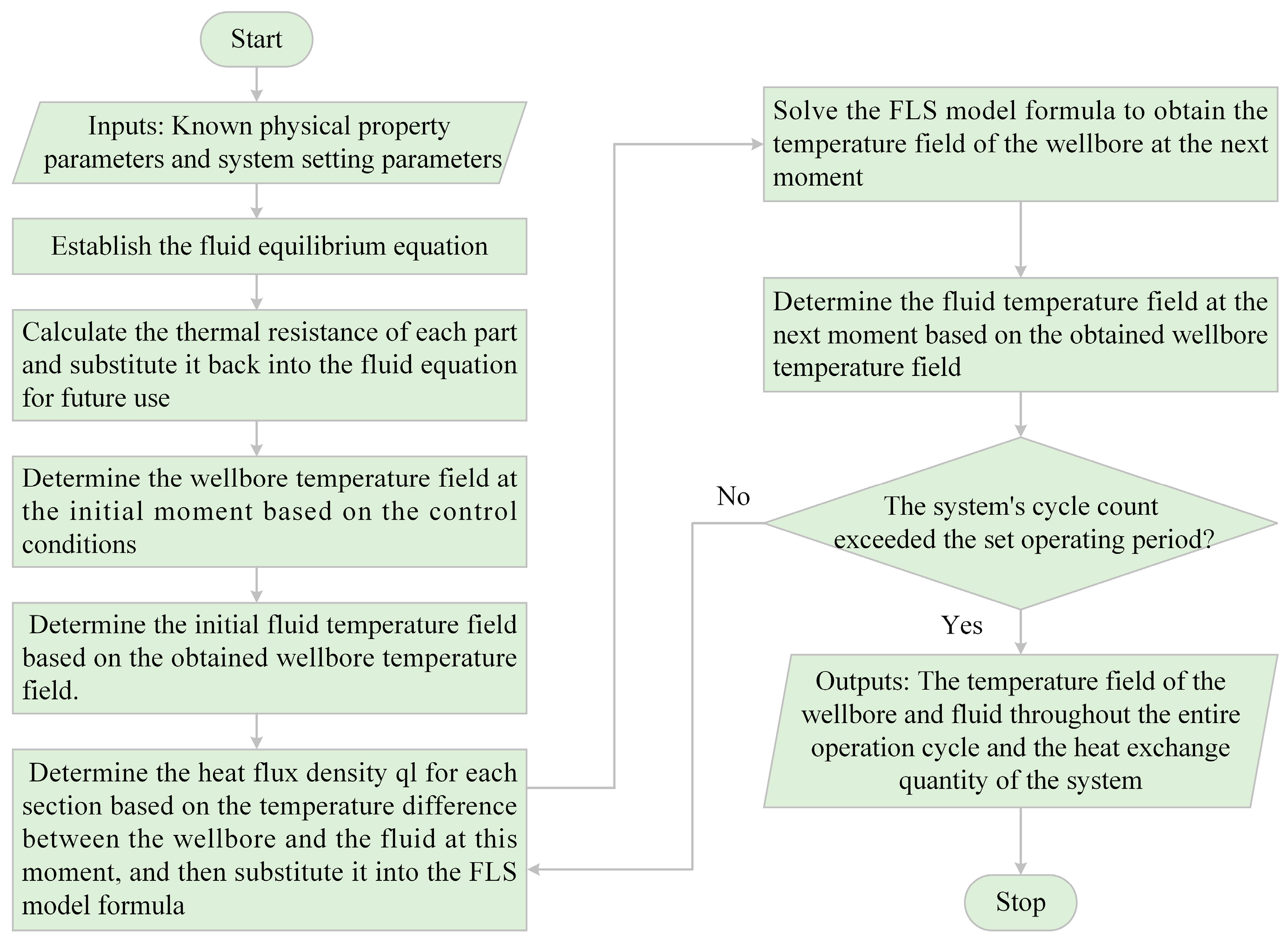
2.2.3. Iterative Calculation Route

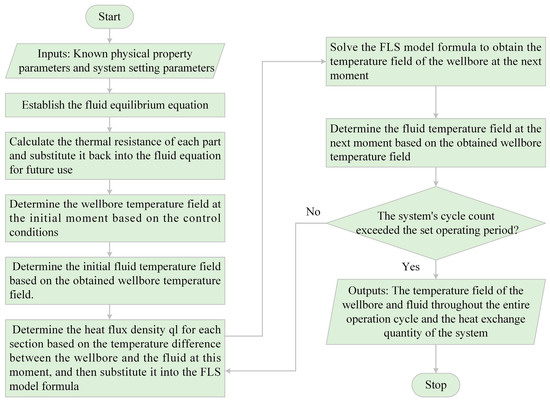
The MATLAB R2023b (version 23.2; The MathWorks, Inc., Natick, MA, USA) implementation uses seconds internally, with reported hours converted using $t_s=3600t_h$. The adopted time step is 1 h, the vertical/horizontal segment lengths are 100/50 m, the convergence tolerance is 10⁻⁴ °C, and the maximum iteration count is 100. Convergence is reached when $\mathrm{m}\mathrm{a}\mathrm{x}\left|T^k-T^{k-1}\right|<{10}^{-4}\hspace{0.17em}°\mathrm{C}$. The validation and parameter-study cases require averages of 6.2 and 7.1 iterations, with maximum observed counts of eight and nine, respectively. The iterative calculation route is shown in Figure 6.

Figure 6. Iterative calculation route. Reproduced from Ref. [46] under the Creative Commons Attribution (CC BY 4.0) license.

3. Results

3.1. Parameter Conditions

Model validation is performed against Bao et al. [49]. The validation case retains the 684 m horizontal section reported by the benchmark, whereas the subsequent parameter and long-term analyses use a 650 m horizontal section. These two geometries are intentionally separated and are described in Section 3.1.

The primary geometric and thermophysical parameters of the UBHE system are summarized in Table 1. For each functional well section—injection, horizontal, and extraction—the hydraulic diameter (D_h) is utilized for hydrodynamic characterization, defined as:

$$D_h={\displaystyle \frac{4A}{P}}$$

(19)

where A denotes the cross-sectional flow area and P represents the wetted perimeter. For the circular conduits investigated in this study, D_h is identically equal to the pipe’s inner diameter. Based on the inner radii provided in Table 1, the calculated values are: D_h = 448 mm for the injection well, D_h = 294 mm for the horizontal well, and D_h = 448 mm for the extraction well.

Table 1. Parameter values used for model validation in this study.

Influencing Factors	Initial Value	Unit
Borehole depth	2500	m
Horizontal tube length	684	m
Outer radius of the injection well	311.7	mm
Outer radius of the horizontal well	168.3	mm
Outer radius of the extraction well	244.5	mm
Inner radius of the injection well	224	mm
Inner radius of the horizontal well	147	mm
Inner radius of the extraction well	224	mm
Thermal capacity of the pipe	3.8 × 106	J/(m3·K)
Thermal conductivity of the pipe	41	W/(m·K)
Volumetric specific thermal capacity of the backfill material	2.5 × 106	J/(m3·K)
Thermal conductivity of the backfill material	1.5	W/(m·K)
Thickness of the insulation layer	18	mm
Length of the insulation layer	200	m
Thermal conductivity of the insulation layer	0.0312	W/(m·K)
Geothermal gradient	0.027	°C/m
Volume flow rate of water	69.81	m3/h
Specific heat capacity of water	4.174 × 103	J/(kg·K)
Average atmospheric temperature	15.7	°C
Characteristic length, $L_c$	10	m

The benchmark study did not report the extraction-well insulation length. Therefore, the validation model uses 200 m and explicitly tests 0, 100, 200, 300, and 400 m. The minimum validation MAE occurs at 200 m, while the limited error variation across the tested range demonstrates that the benchmark agreement is not determined solely by this assumption.

Table 2 and Table 3 list the thermophysical parameters for the rock-soil and fluid phases. Equivalent thermophysical properties for each geological layer are calculated via Equations (9) and (10), incorporating seepage effects and stratification into the heat transfer simulation.

Table 2. Thermophysical parameters of the rock-soil matrix under stratified geological conditions [49].

Sequence	Depth m	Volumetric Specific Heat Capacity (J/(m3·K))	Thermal Conductivity (W/(m·K))	Porosity (%)
1	0–420	1.379 × 106	1.8	0.47
2	420–1000	1.3 × 106	3.5	0.31
3	1000–1580	1.45 × 106	2.6	0.33
4	1580–2300	1.45 × 106	2.6	0.475
5	2300–2500	1.45 × 106	2.6	0.18

Table 3. Seepage parameters under stratified geological conditions.

Sequence	Depth m	Water Temperature at the Respective Depths (°C) (${\mathit{k}}_{\mathbf{g}\mathbf{e}\mathbf{o}}=0.027\hspace{0.17em}°\mathbf{C}/\mathbf{m}$, ${\mathit{T}}_0=15.7\hspace{0.17em}°\mathbf{C}$)	Thermal Conductivity (W/(m·K))	Seepage Velocity (m/s)
1	0–420	27.04	0.6	2.2 × 10−12
2	420–1000	42.70	0.62	3 × 10−6
3	1000–1580	58.36	0.64	4.2 × 10−8
4	1580–2300	77.80	0.66	1.4 × 10−9
5	2300–2500	82.30	0.67	4.2 × 10−10

The differences between the validation and parameter-study configurations are summarized in Table 4.

Table 4. Geometric and numerical distinction between the validation and parameter-study cases.

Item	Validation Case	Parameter-Study Case
Vertical well depth	2500 m	2500 m
Horizontal-section length	684 m	650 m
Baseline insulation length	200 m	1600 m for the optimized case
Geothermal gradient	0.027 °C/m	0.027 °C/m baseline; 0.01–0.04 °C/m in the gradient study
Simulation duration	720 h	8760 h for annual analyses; 10 years for long-term analyses
Purpose	Comparison with Bao et al. [49]	Mechanism, optimization, and sensitivity analyses

3.2. Comparison of Simulation Results

Model-reference agreement is quantified by $MAE={\displaystyle \frac{1}{N}}\sum \left|T_{\mathrm{o}\mathrm{u}\mathrm{t},\mathrm{m}\mathrm{o}\mathrm{d}\mathrm{e}\mathrm{l}}-T_{\mathrm{o}\mathrm{u}\mathrm{t},\mathrm{r}\mathrm{e}\mathrm{f}}\right|$, $RMSE={\left[{\displaystyle \frac{1}{N}}\sum {\left(T_{\mathrm{o}\mathrm{u}\mathrm{t},\mathrm{m}\mathrm{o}\mathrm{d}\mathrm{e}\mathrm{l}}-T_{\mathrm{o}\mathrm{u}\mathrm{t},\mathrm{r}\mathrm{e}\mathrm{f}}\right)}^2\right]}^{1/2}$, the maximum absolute error, and ${\epsilon }_T={\displaystyle \frac{\left|T_{\mathrm{o}\mathrm{u}\mathrm{t},\mathrm{m}\mathrm{o}\mathrm{d}\mathrm{e}\mathrm{l}}-T_{\mathrm{o}\mathrm{u}\mathrm{t},\mathrm{r}\mathrm{e}\mathrm{f}}\right|}{T_{\mathrm{o}\mathrm{u}\mathrm{t},\mathrm{r}\mathrm{e}\mathrm{f}}}}\times 100\mathrm{\%}$. All sensitivity calculations use the same definitions.

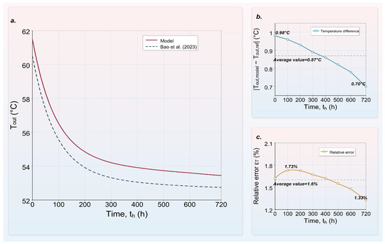
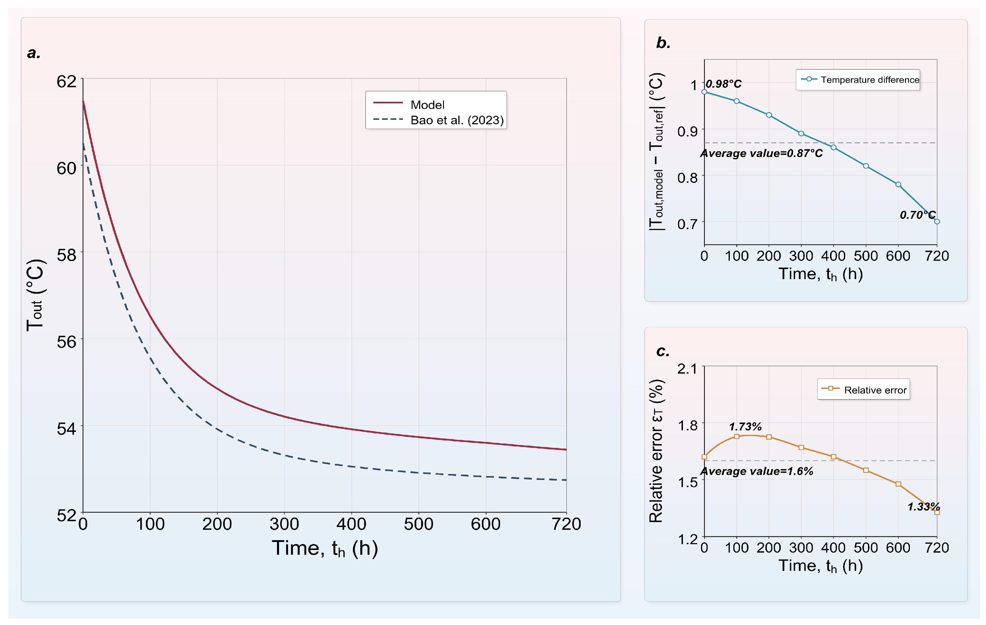
The comparative results are presented in Figure 7. As shown in Figure 7a, the outlet water temperature experiences a rapid decline during the initial operational phase before stabilizing at a plateau. After 200 h, the relative outlet-temperature error ε_T falls below 2% and exhibits a continuous decreasing trend, reaching its minimum by the end of the simulation.

Figure 7. (a) Comparison of outlet temperatures. (b) Temperature difference. (c) Relative outlet-temperature error ε_T. Panel (c) is replotted using ε_T per the definition above. Reference data are from Bao et al. [49].

Across the benchmark period, the maximum absolute temperature deviation is 0.98 °C, the MAE is 0.87 °C, and the mean relative outlet-temperature error is 1.6%. These values demonstrate close agreement with the reference results while remaining explicitly tied to the Bao et al. benchmark, rather than being presented as field validation.

The uncertainty of the benchmark comparison is evaluated directly through the numerical-independence and parameter-sensitivity analyses in Section 4.4.

The time-step, spatial-segmentation, and iterative-convergence tests quantify numerical implementation effects.

Equivalent conductivity, geothermal gradient, seepage velocity, and validation insulation length are varied explicitly to quantify parameter sensitivity.

The corresponding numerical-independence, limiting-case, and parameter-sensitivity analyses are presented in Section 4.4.1, Section 4.4.2 and Section 4.4.3; the previous unsupported statement that the uncertainty was merely within a few percent’ is removed.

3.3. Spatiotemporal Evolution of the Fluid Temperature Field

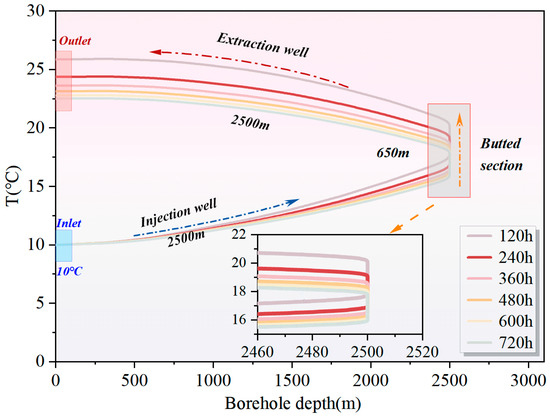
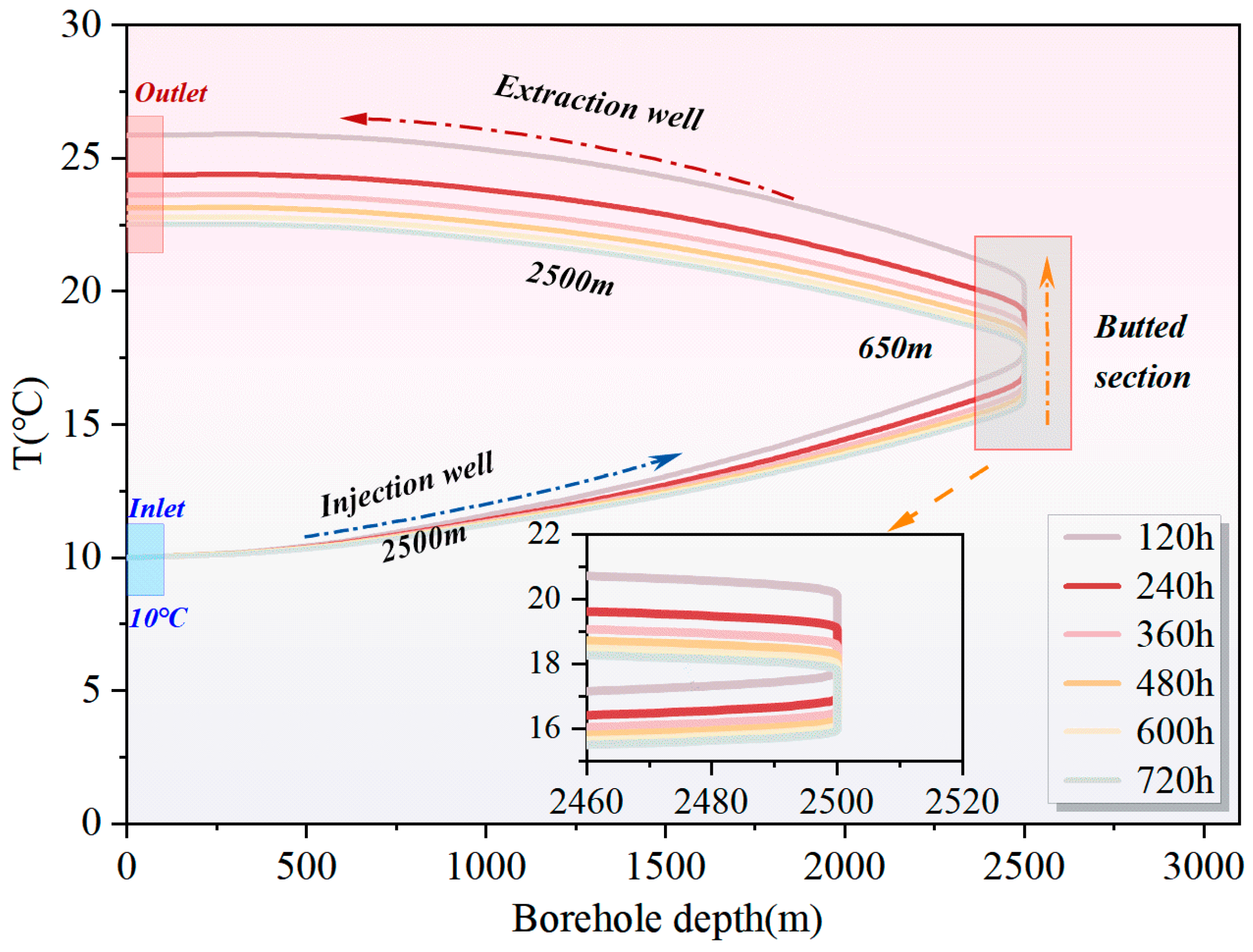
Figure 8 illustrates the temperature profile for the parameter-study geometry, consisting of a 2500 m injection well, a 650 m horizontal section, and a 2500 m extraction well. This geometry is distinct from the 684 m benchmark configuration. The vertical and horizontal sections are discretized into 100 and 50 m segments, respectively.

Figure 8. Fluid temperature fields at different times.

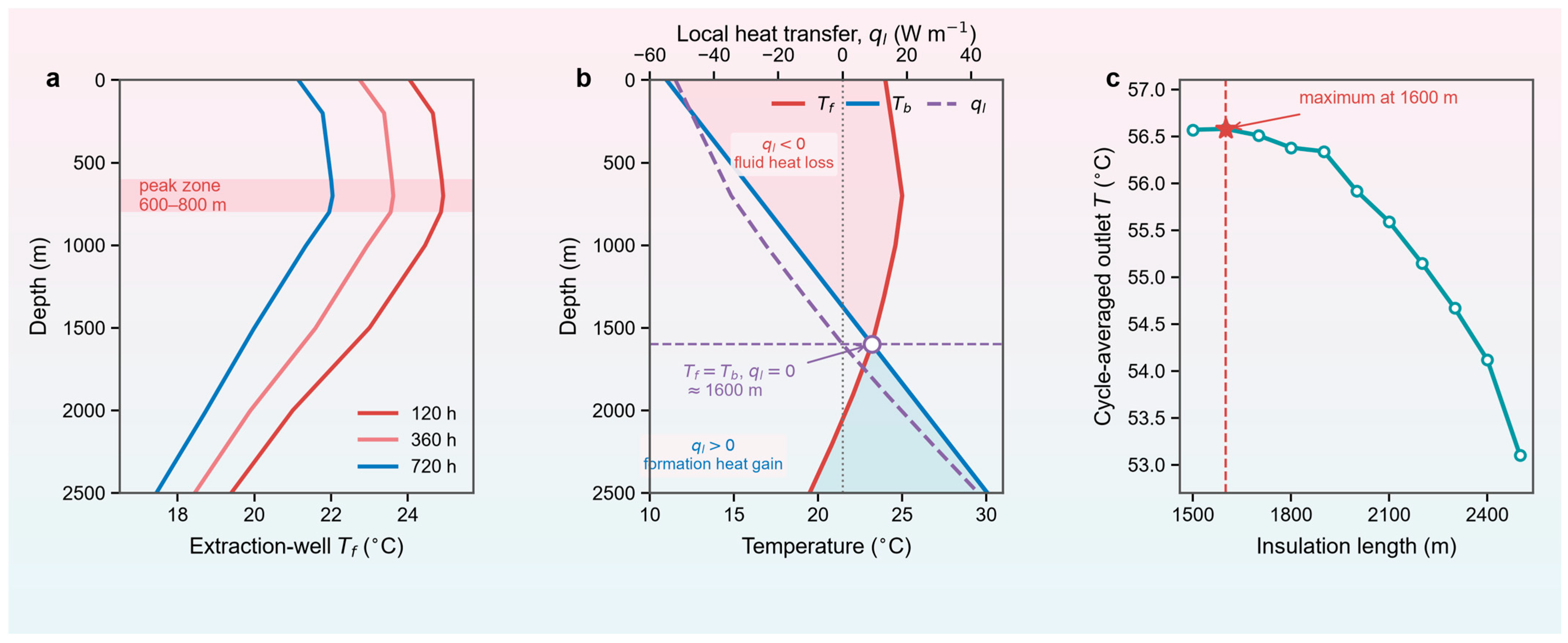
The fluid-temperature maximum occurs at 600–800 m depth in the extraction well rather than at the bottom. This temperature peak is a spatial maximum of $T_f$. It is distinct from the approximately 1600 m location where $T_f=T_b$ and $q_l$ changes sign. In the shallow extraction-well section, $T_f$ exceeds $T_b$ and the fluid loses heat to the formation; deeper than the crossover, the formation supplies heat to the fluid.

The thermal response is higher at 120 h, with profiles shifting downward by 720 h due to thermal depletion. The narrowing gap between successive temporal curves (e.g., 120–240 h vs. 600–720 h) indicates a transition from transient to quasi-steady state.

4. Discussion

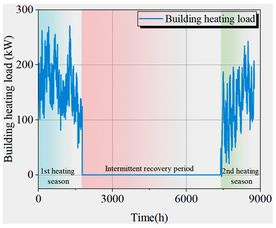
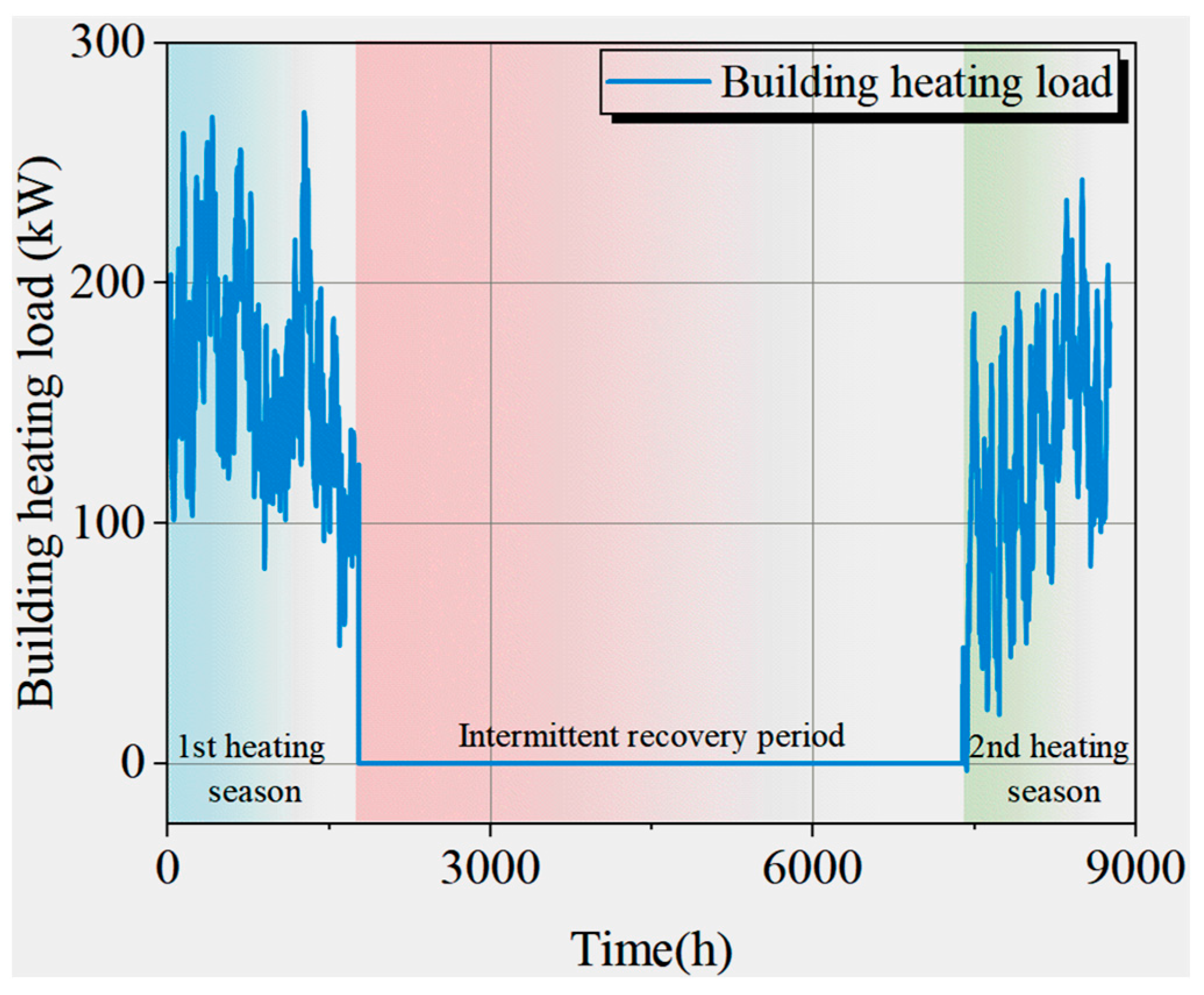
Long-term performance over one year is evaluated using the prescribed seasonal building-load profile shown in Figure 9. The flow rate remains fixed, while inlet and outlet temperatures evolve from the load relation and coupled UBHE equations.

Figure 9. Heating load profile within a single heating season.

4.1. Effects of Geothermal Gradient

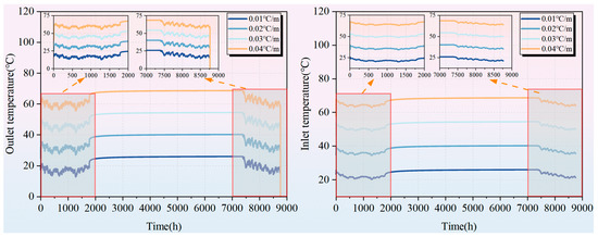
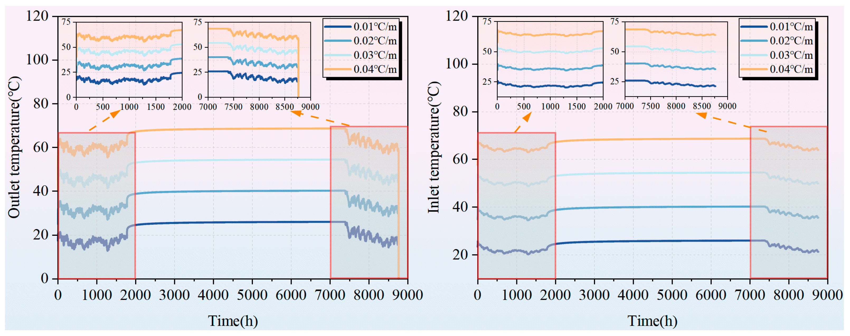
Geothermal gradients from 0.01 to 0.04 °C/m, based on data from the Songliao Basin, North China Basin, and basins in South China [50,51], were used for an 8760 h simulation. Between 2000 h and 7000 h, a 0.01 °C/m gradient results in an average outlet temperature of 25 °C, while a 0.04 °C/m gradient results in 68 °C. Temperature fluctuations during the periods 0–2000 h and 7000–9000 h occur across all gradients. The corresponding inlet- and outlet-temperature responses are shown in Figure 10.

Figure 10. Effects of geothermal gradient on the outlet temperature and inlet temperature.

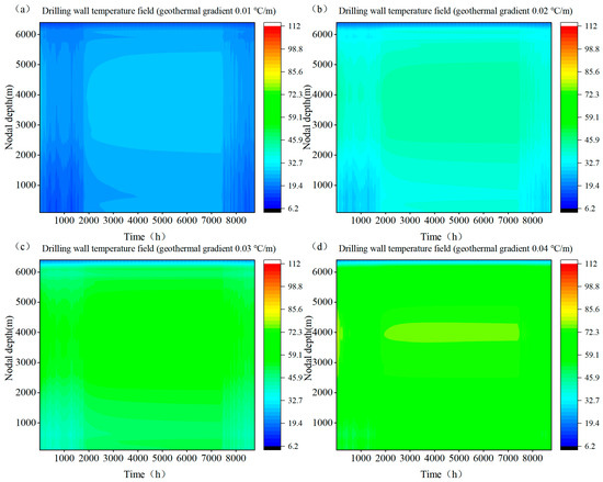
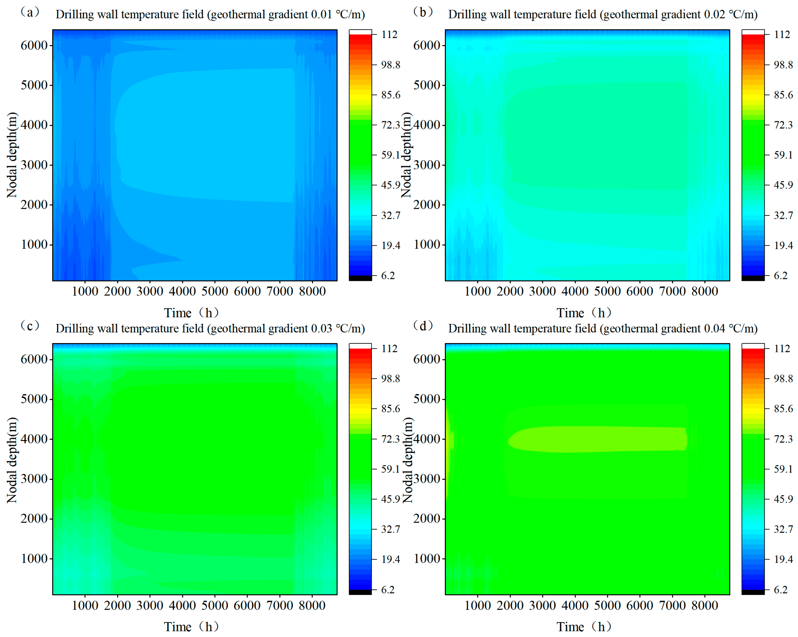
Figure 11 illustrates the spatiotemporal evolution of the borehole wall temperature field. With higher geothermal gradients, high-temperature regions in the deep strata (indicated by red and yellow contours) expand significantly, with bottom-hole temperatures reaching approximately 85.6 °C. The increased temperature differential between the pristine formation and the circulating fluid enhances the radial thermal driving force, facilitating heat extraction along the horizontal section. Consequently, the geothermal gradient directly influences the thermodynamic limit of extractable energy and serves as a key parameter for geological surveys and techno-economic feasibility evaluations.

Figure 11. Spatiotemporal evolution of the bore hole wall temperature field under different geothermal gradients.

4.2. Impact of Insulation Layer Length Under Long-Term Cyclic Operation

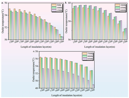
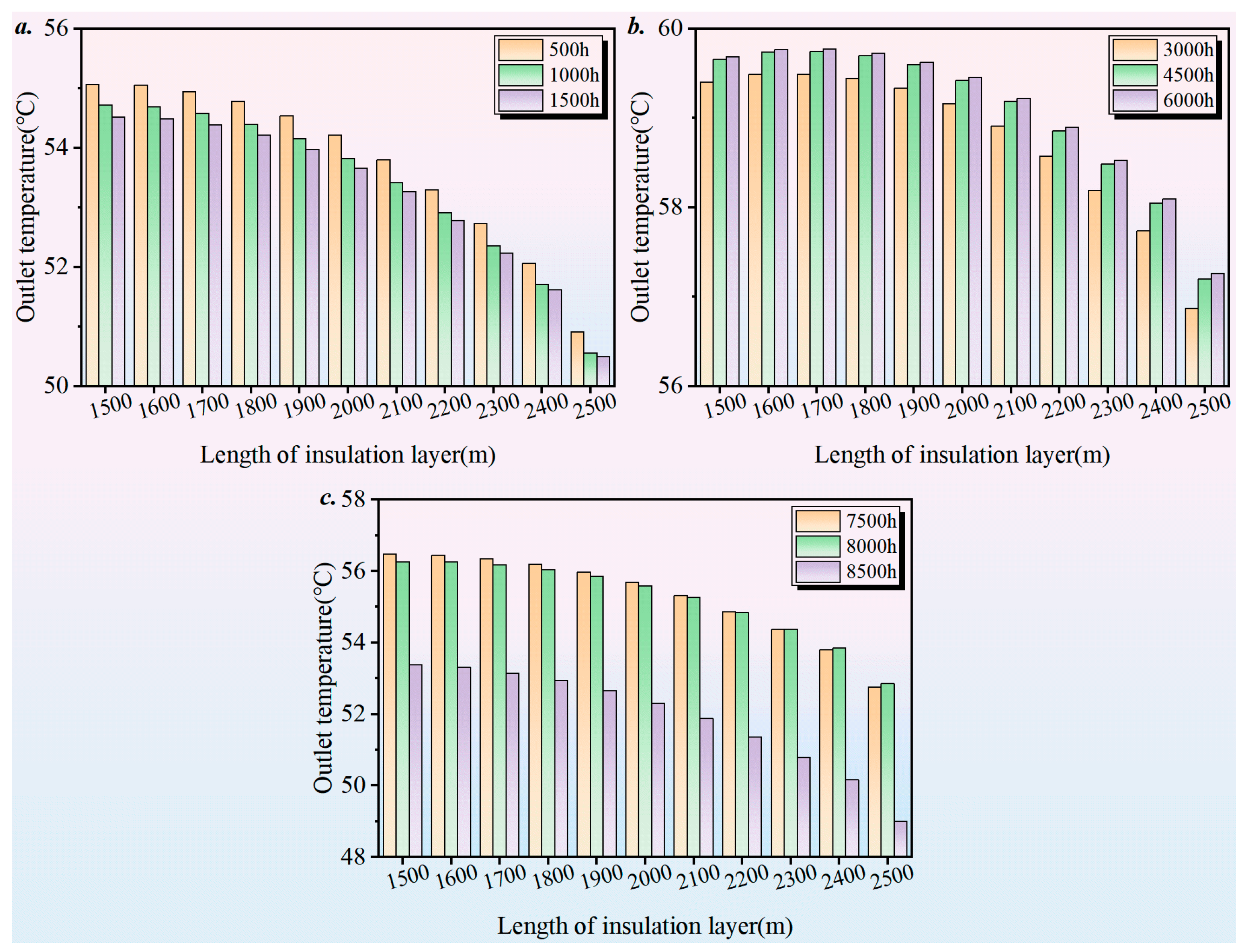
This section evaluates extraction-well insulation lengths from 1500 to 2500 m during the first heating season, intermittent recovery period, and second heating season. The optimization objective is the cycle-averaged outlet temperature under the prescribed load profile.

As shown in Figure 12a–c, although absolute outlet temperatures fluctuate periodically due to seasonal thermal depletion and recovery, the dependence of the outlet temperature on the insulation length remains consistent across all operational phases. This indicates that the insulation mechanism is independent of the operational time scale.

Figure 12. (a–c) Effects of the insulation layer on the outlet temperature at different running times.

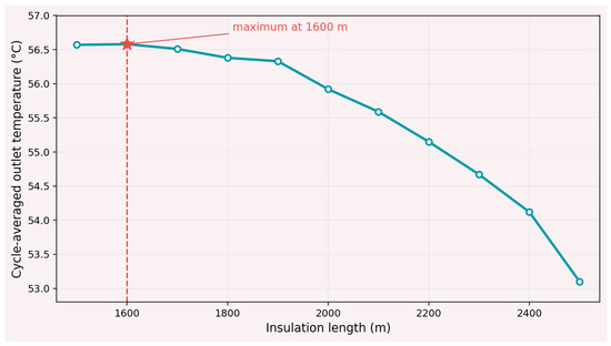
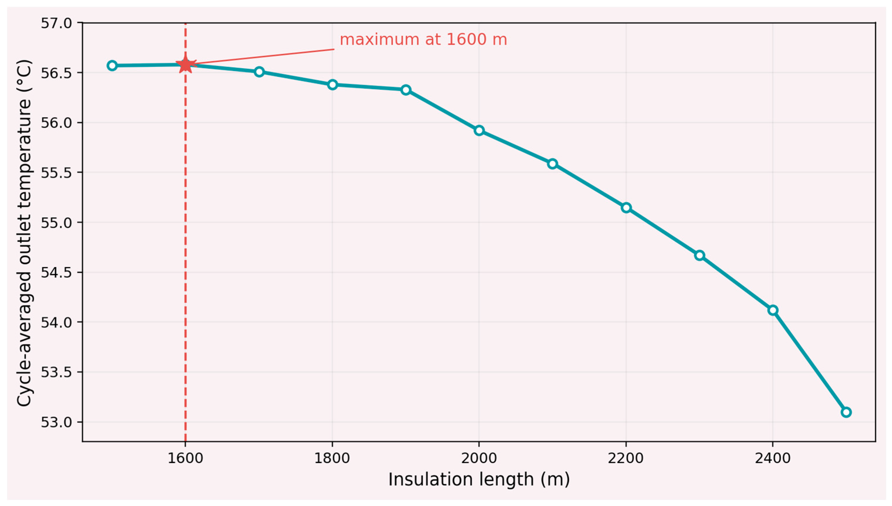
Figure 13 summarizes the cycle-averaged outlet temperature. Among the investigated discrete cases, 1600 m produces the maximum value of 56.58 °C. The 1500–1700 m results are close, but the outlet temperature decreases progressively when insulation extends farther into the deeper heat-gain region, reaching 53.10 °C under full insulation.

Figure 13. Cycle-averaged outlet temperature for the investigated extraction-well insulation lengths.

The physical relationship among the temperature peak, heat-transfer crossover, and optimum insulation length is discussed in Section 4.4.4. The 600–800 m peak is the maximum of the fluid-temperature profile, whereas the approximately 1600 m crossover is defined by $T_f=T_b$ and $q_l=0$. Insulation above the crossover suppresses fluid heat loss to shallow formations; insulation extending below the crossover blocks beneficial heat gain from deeper formations. Consequently, the cycle-integrated optimum occurs at 1600 m for the present geometry, but it is not a universal fixed depth. The corresponding dimensionless insulation ratio is $L_{\mathrm{o}\mathrm{p}\mathrm{t}}/H=1600/2500=0.64$.

4.3. Sensitivity Analysis of Geological Thermophysical Properties

4.3.1. Comparative Analysis Between Stratified and Homogeneous Geological Assumptions

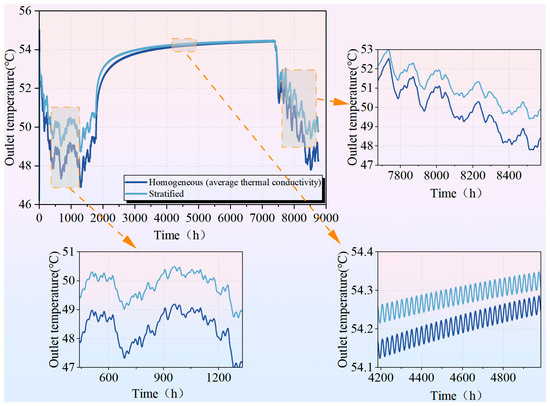
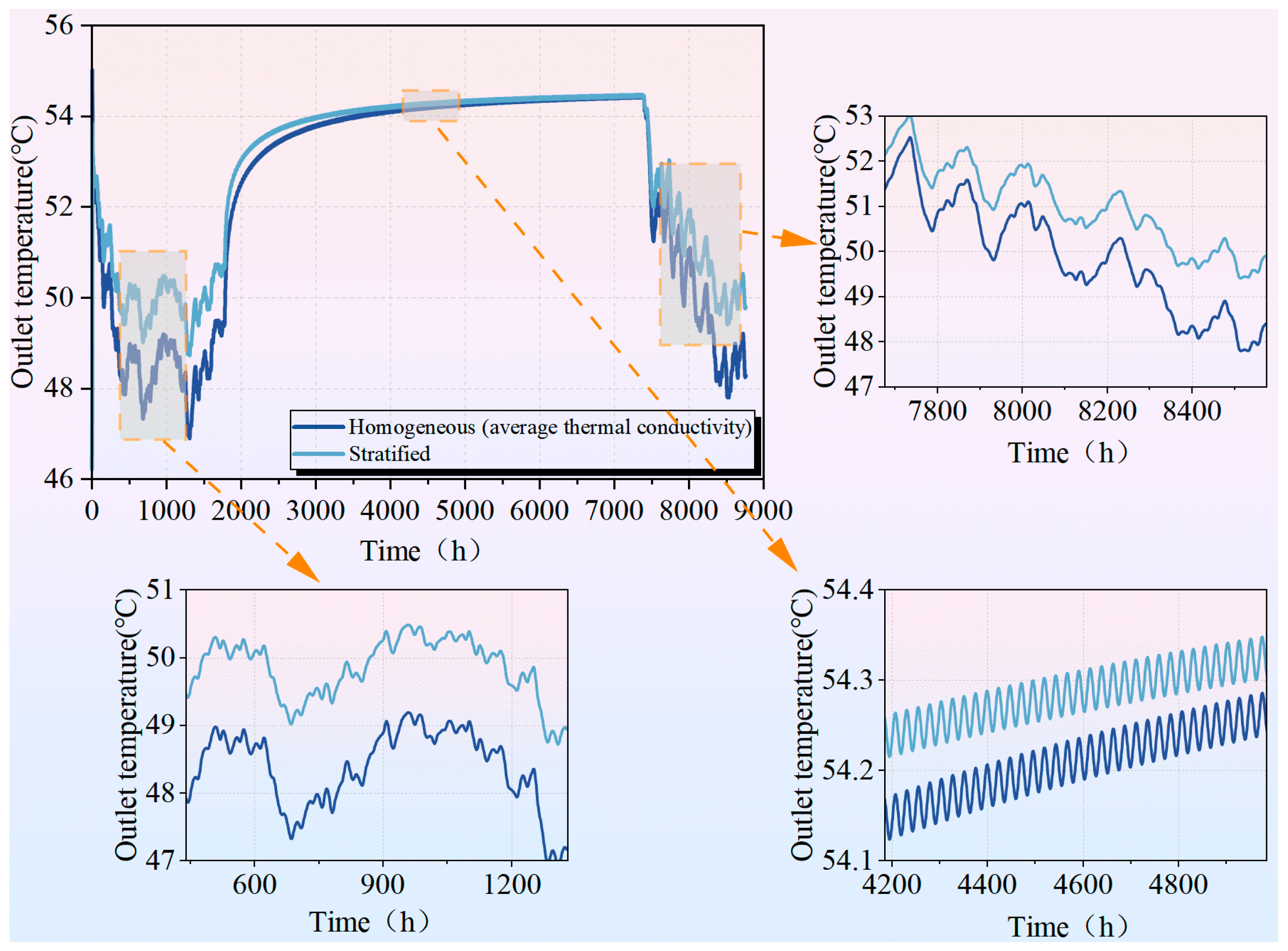
To evaluate the necessity of a multi-layered analytical model, this section compares the outlet water temperature over a one-year cycle (8760 h) under two assumptions: a realistic stratified geological model and a homogeneous model. The latter utilizes a depth-weighted average thermal conductivity to represent the entire formation.

Both models reflect seasonal thermal drawdown and recovery. However, the stratified model predicts higher outlet temperatures than the homogeneous model, specifically during heat extraction.

(i)

First Heating Season (400–1300 h): The stratified model outlet temperature ranges from 49.0 to 50.5 °C, while the homogeneous model remains between 47.5 and 49.0 °C, a difference of approximately 1.5 °C.

(ii)

Intermittent Period (4200–5000 h): The temperature gap reduces to less than 0.1 °C. Both models reach a recovery ceiling of 54.2–54.4 °C.

(iii)

Second Heating Season (7600–8600 h): The gap returns to 1.0–1.5 °C. Temperatures in both models are lower than the first season due to reservoir thermal depletion.

The homogeneous model uses depth-weighted averages for thermal conductivity and initial temperature. The 650 m horizontal section is located at 2500 m, where local thermophysical parameters exceed these depth-averaged values. The stratified model applies local parameters to this section, whereas the homogeneous model applies averaged values, resulting in lower predicted heat extraction rates for the latter. The long-term comparison is shown in Figure 14.

Figure 14. Long-term dynamic comparison of system outlet water temperature under stratified and homogeneous geological assumptions.

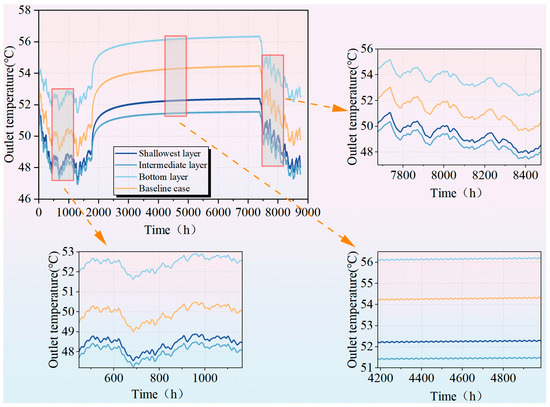
4.3.2. Sensitivity Analysis of Thermal Conductivity Variations Across Different Geological Strata

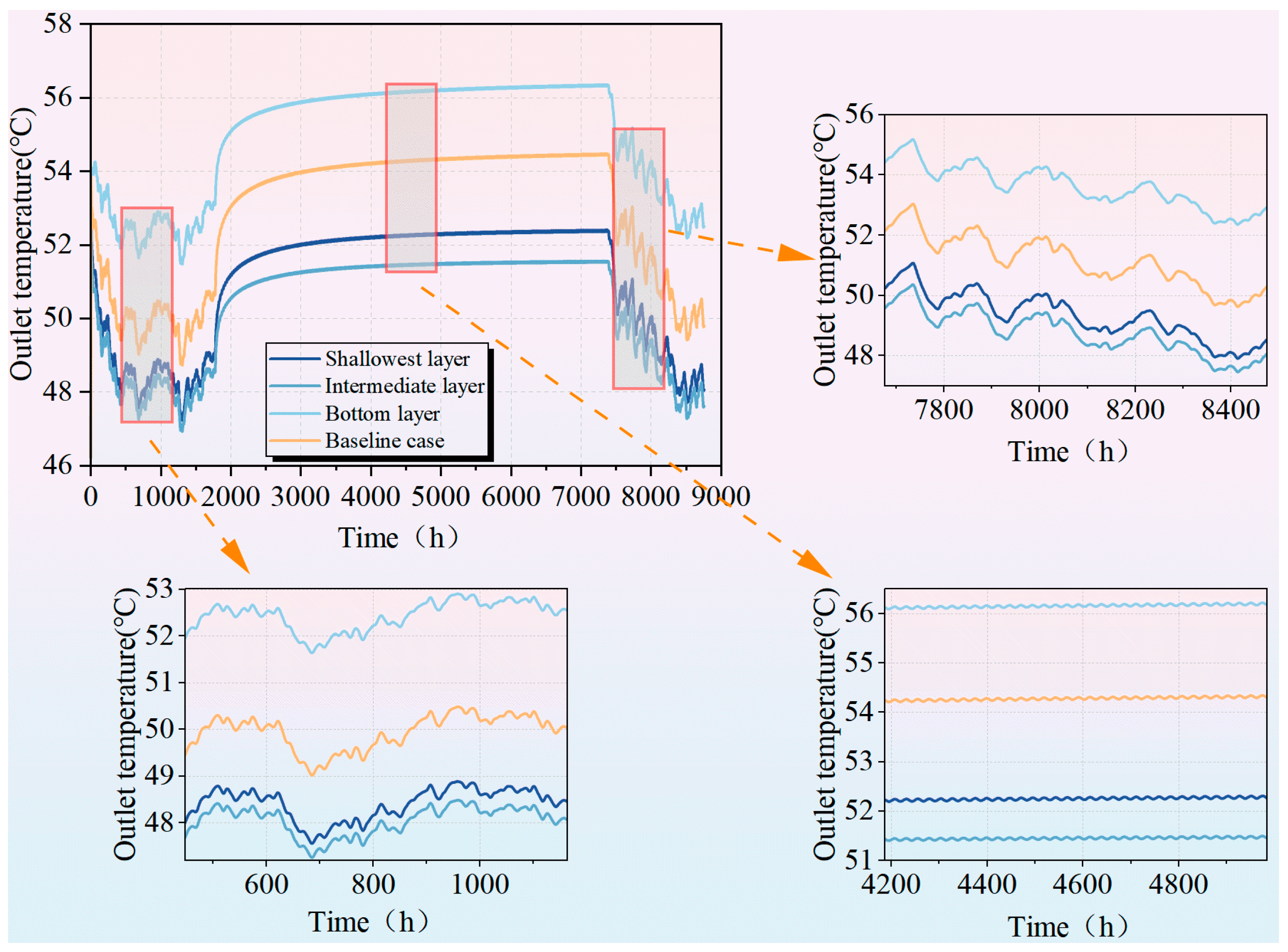
To further elucidate the regulatory mechanism of geological heterogeneity on the performance of the UBHE, this section evaluates the effect of thermal conductivity in the shallow (0–400 m), intermediate (400–1000 m), and bottom (2300–2500 m) layers on the outlet water temperature. Figure 15 shows the simulation results for an 8760 h cycle and includes magnified views of operational phases.

Figure 15. Long-term dynamic comparison of system outlet water temperature under different thermal conductivity.

(i)

First Heating Season (500–1400 h): Increasing thermal conductivity in the bottom layer (2300–2500 m) results in an outlet temperature of 52.5 °C, compared to the baseline of 50.2 °C. This layer contains the 650 m horizontal section. Increased conductivity reduces radial thermal resistance at this depth. Increasing conductivity in the shallow (0–400 m) and intermediate (400–1000 m) layers results in outlet temperatures of 48.4 °C and 48.1 °C. In these layers, fluid temperature exceeds formation temperature, and increased conductivity leads to heat loss from the fluid to the strata.

(ii)

Intermittent Recovery Period (4200–5000 h): Temperature differences between cases decrease. The gap between the bottom-layer enhancement and the baseline reduces to 1.8 °C. Curves converge, indicating that thermal conductivity variations have a reduced influence on the static thermal recovery limit.

(iii)

Second Heating Season (7600–8600 h): The temperature hierarchy remains consistent with the first season. The baseline outlet temperature is 50.1 °C, a 0.1 °C decrease from the first season. Temperatures for the shallow and intermediate enhancement cases reach 48.2 °C and 47.9 °C, representing a 0.2 °C decrease relative to the first season.

The opposite effects of layer conductivity follow from the local sign of $q_l\propto T_b-T_f$. In deep formations, $T_b>T_f$, and higher conductivity strengthens heat supply to the fluid. In shallow formations, $T_f>T_b$, and higher conductivity intensifies reverse heat loss. Thus, deep-layer conductivity governs useful heat extraction, whereas shallow-layer insulation limits parasitic dissipation.

4.3.3. Regulatory Mechanism of Thermal Inertia on Long-Term Thermal Drawdown

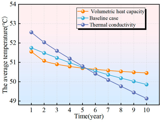
Thermal sustainability is crucial for the long-term operation of borehole heat exchangers. While thermal conductivity governs transient heat transfer rates, volumetric heat capacity plays a key role in thermal inertia and long-term temperature drawdown. This section compares their impacts over a 10-year simulation period and introduces a Sustainability Index (SI) to quantify the buffering effect against thermal exhaustion.

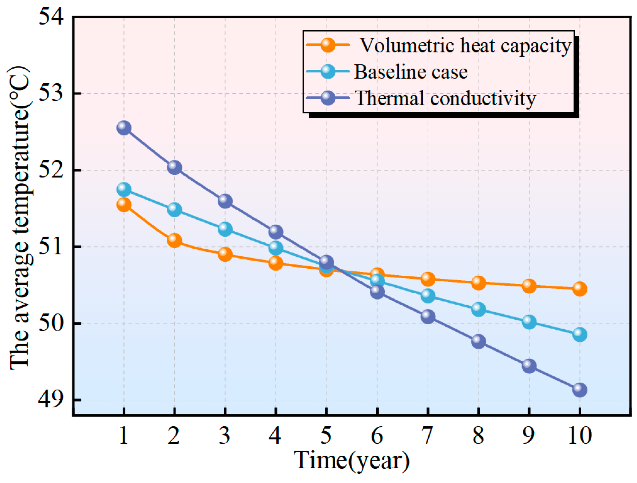
Figure 16 illustrates the 10-year evolution of the average outlet temperature. In the first year of operation, the enhanced thermal conductivity case exhibits the highest outlet temperature at 52.55 °C, while the baseline and enhanced volumetric heat capacity cases are 51.75 °C and 51.55 °C, respectively.

Figure 16. Outlet temperature evolution: conductivity, heat capacity and baseline case.

However, the cases exhibit distinct temperature drawdown rates. The enhanced thermal conductivity case shows the most significant decline, dropping to 49.13 °C by the tenth year with a total decrease of 3.42 °C. In contrast, the volumetric heat capacity case demonstrates the highest thermal stability, with the temperature decreasing from 51.55 °C to 50.45 °C, a total drop of only 1.10 °C. The temperature drawdown for the baseline case is 1.89 °C (from 51.75 °C to 49.86 °C).

A critical performance crossover is observed at approximately year 5.4. Beyond this point, the performance of the thermal conductivity case falls below the baseline. This trend indicates that while high thermal conductivity enhances heat exchange initially, it leads to the excessive extraction of heat from the deep reservoir, termed the “thermal overdraft” effect. Conversely, the volumetric heat capacity effectively delays the thermal exhaustion process by providing higher geological thermal inertia, ensuring the long-term heat production potential of the system.

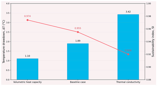
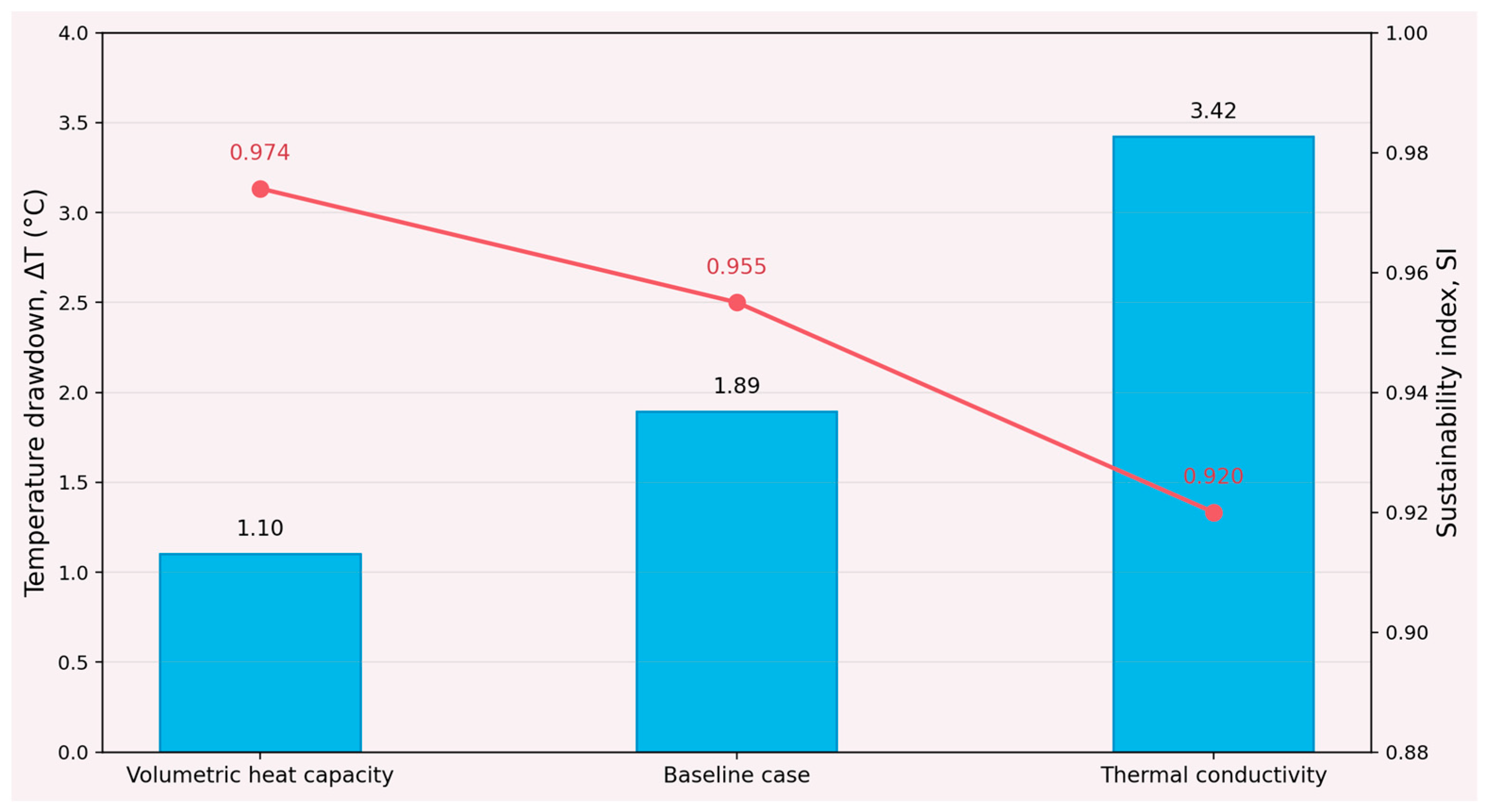
Figure 17 compares the outlet-temperature drawdown between the first and tenth years and the revised Sustainability Index (SI) for each case.

Figure 17. Corrected ten-year outlet-temperature drawdown and Sustainability Index.

SI is defined as the retention ratio of the cycle-averaged effective temperature rise during the same heating period in Years 10 and 1: $SI={\displaystyle \frac{{\overline{T}}_{\mathrm{o}\mathrm{u}\mathrm{t},\mathrm{y}\mathrm{e}\mathrm{a}\mathrm{r}10}-{\overline{T}}_{\mathrm{i}\mathrm{n},\mathrm{y}\mathrm{e}\mathrm{a}\mathrm{r}10}}{{\overline{T}}_{\mathrm{o}\mathrm{u}\mathrm{t},\mathrm{y}\mathrm{e}\mathrm{a}\mathrm{r}1}-{\overline{T}}_{\mathrm{i}\mathrm{n},\mathrm{y}\mathrm{e}\mathrm{a}\mathrm{r}1}}}$. The same averaging interval and inlet-temperature definition are used in both years, so the metric is dimensionless and directly reproducible without an undefined asymptotic temperature.

$$SI={\displaystyle \frac{{\overline{T}}_{\mathrm{o}\mathrm{u}\mathrm{t},\mathrm{y}\mathrm{e}\mathrm{a}\mathrm{r}10}-{\overline{T}}_{\mathrm{i}\mathrm{n},\mathrm{y}\mathrm{e}\mathrm{a}\mathrm{r}10}}{{\overline{T}}_{\mathrm{o}\mathrm{u}\mathrm{t},\mathrm{y}\mathrm{e}\mathrm{a}\mathrm{r}1}-{\overline{T}}_{\mathrm{i}\mathrm{n},\mathrm{y}\mathrm{e}\mathrm{a}\mathrm{r}1}}}$$

(20)

With a cycle-averaged inlet temperature of 10.00 °C, the revised SI values are 0.974 for the enhanced volumetric-heat-capacity case, 0.955 for the baseline, and 0.920 for the enhanced-conductivity case.

The enhanced volumetric-heat-capacity case has the smallest ten-year outlet-temperature drawdown of 1.10 °C. The baseline drawdown is 1.89 °C, and the enhanced-conductivity case has the largest drawdown of 3.42 °C. These values are consistent with Figure 16 and replace the previous inconsistent values.

The revised SI values confirm that increased volumetric heat capacity provides the strongest long-term thermal buffering, whereas increased conductivity improves initial heat transfer but accelerates reservoir drawdown. The complete values are listed in Table 5.

Table 5. Corrected ten-year temperature drawdown and Sustainability Index.

Case	Year-1 Mean Outlet Temperature (°C)	Year-10 Mean Outlet Temperature (°C)	Drawdown (°C)	SI
Baseline	51.75	49.86	1.89	0.955
Enhanced thermal conductivity	52.55	49.13	3.42	0.920
Enhanced volumetric heat capacity	51.55	50.45	1.10	0.974

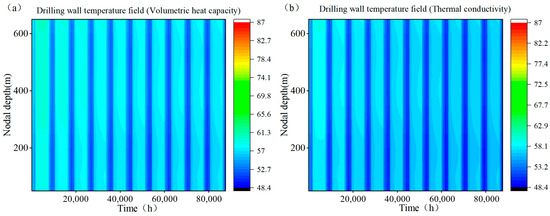
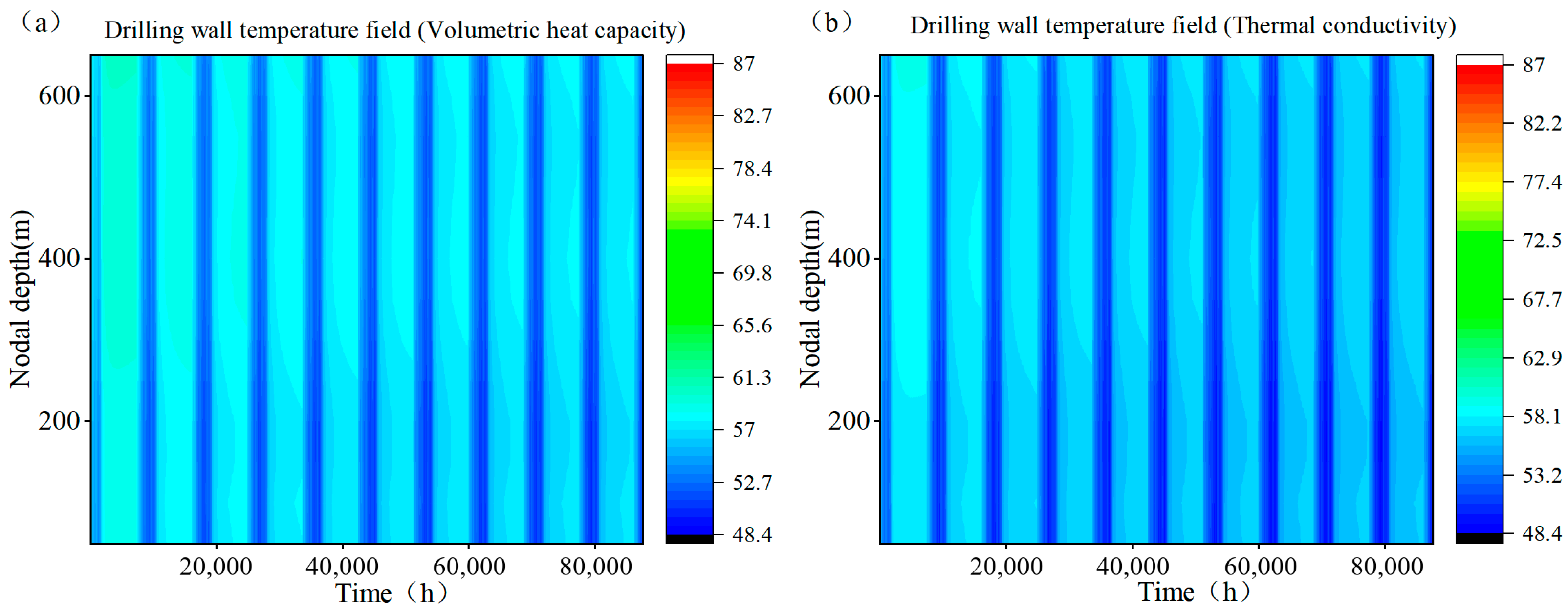
Figure 18 illustrates the spatiotemporal evolution of the borehole wall temperature field along the horizontal section over the 10-year operational period.

Figure 18. Horizontal borehole wall temperature distribution.

Comparing Figure 18a,b, the rate and magnitude of the temperature drop at the borehole wall in the thermal conductivity case (b) are higher than those in the volumetric heat capacity case (a). During active cycles, the low-temperature regions (dark blue bands) in the conductivity case are more intense, indicating a more rapid decline in near-wellbore formation temperatures.

This indicates that higher thermal conductivity accelerates local energy depletion, leading to rapid exhaustion of the thermal reservoir near the wellbore. In contrast, the volumetric heat capacity case maintains higher wall temperatures through superior thermal inertia, decelerating the energy exhaustion process at the heat exchange interface.

4.4. Model Reliability, Robustness, and Mechanistic Verification

4.4.1. Numerical Independence and Convergence

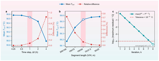
Time steps of 0.25, 0.5, 1, 2, and 4 h and vertical/horizontal segment lengths of 200/100, 150/75, 100/50, 75/37.5, and 50/25 m were compared. The 1 h and 100/50 m settings provide changes below 0.1% relative to the finest reference cases and are adopted for all reported simulations. The representative residual decreases monotonically and falls below 10⁻⁴ °C at the eighth iteration. The adopted numerical settings are summarized in Table 6, and the corresponding independence and convergence results are shown in Figure 19.

Table 6. Numerical implementation settings used in the final calculations.

Setting	Validation Case	Parameter-Study Case
Simulation duration	720 h	8760 h
Time step	1 h	1 h
Injection/extraction segment length	100 m	100 m
Horizontal segment length	50 m	50 m
Convergence variable	max|Tk − Tk−1|	max|Tk − Tk−1|
Tolerance	10−4 °C	10−4 °C
Maximum allowed iterations	100	100
Mean iterations	6.2	7.1
Maximum observed iterations	8	9
Internal time unit	s	s

Figure 19. Numerical independence and convergence analysis. (a) Effect of time-step size on the mean outlet temperature and relative difference with respect to the 0.25 h result. (b) Effect of vertical/horizontal segment lengths and relative difference with respect to the 50/25 m result. (c) Maximum temperature residual versus iteration number; convergence is reached below 10⁻⁴ °C. The red shaded regions indicate the adopted numerical settings (Δt = 1 h and vertical/horizontal segment lengths of 100/50 m).

4.4.2. Analytical Limiting-Case Verification

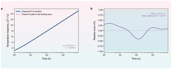
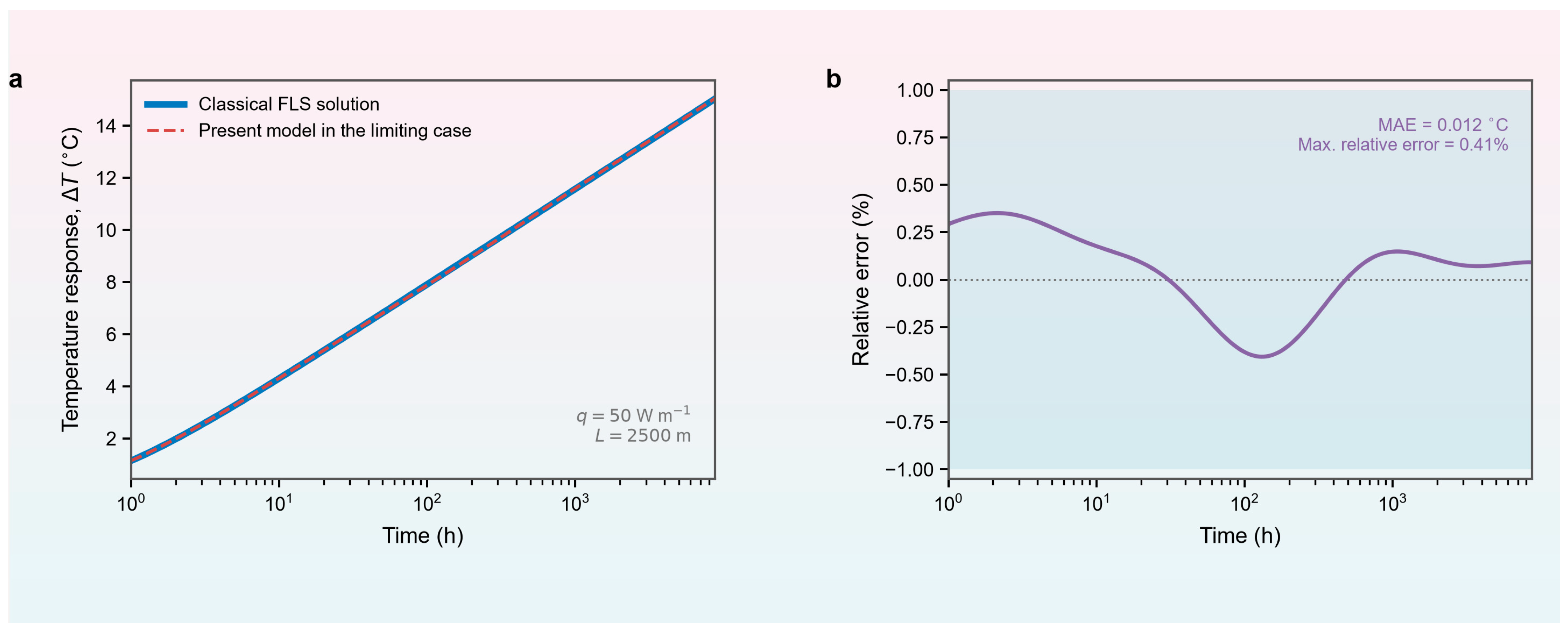
For an independent analytical check, the present model is reduced to a single 2500 m finite line source in a homogeneous formation with zero seepage, zero geothermal gradient, no insulation, and $q_l=50\hspace{0.17em}\mathrm{W}/\mathrm{m}$. The resulting 1–8760 h response is compared with the classical finite line-source solution. The curves overlap closely, with an MAE of 0.012 °C and a maximum relative-error magnitude of 0.41%. The comparison is shown in Figure 20 and summarized in Table 7.

Figure 20. Analytical limiting-case verification against the classical finite line-source solution. (a) Temperature responses predicted by the classical FLS solution and the present model. (b) Signed relative error over time.

Table 7. Summary of the classical FLS limiting-case verification.

Metric	Result	Acceptance Criterion	Assessment
MAE	0.012 °C	<$0.10\hspace{0.17em}°\mathrm{C}$	Pass
Maximum relative-error magnitude	0.41%	<$1\mathrm{\%}$	Pass

4.4.3. Parameter Sensitivity and Validation Robustness

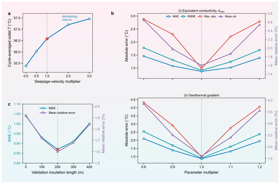
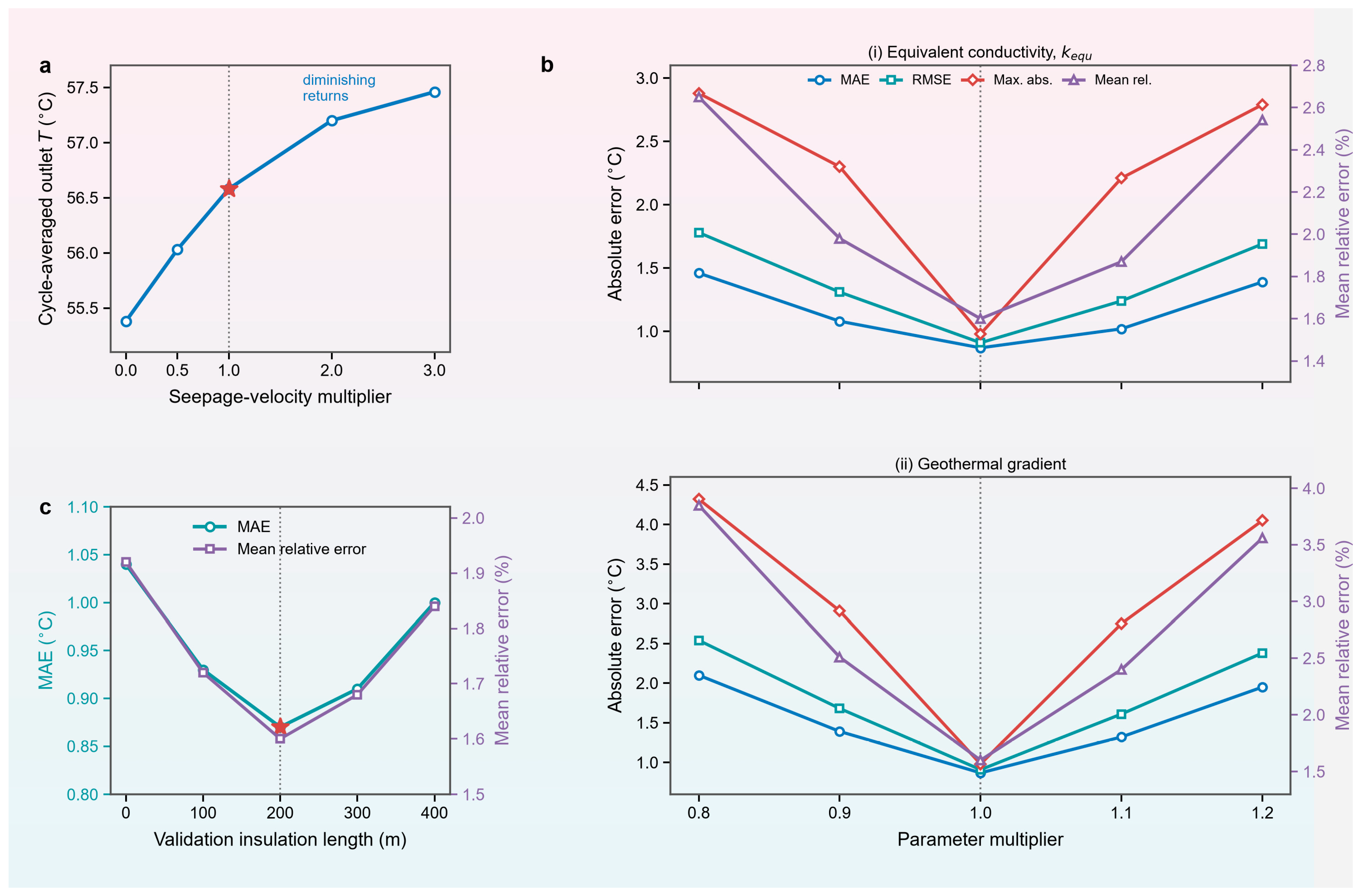
The seepage velocity is multiplied by 0, 0.5, 1, 2, and 3. Equivalent conductivity and geothermal gradient are varied from 0.8 to 1.2 times their baseline values, and the validation insulation length is varied from 0 to 400 m. Seepage raises the cycle-averaged outlet temperature with diminishing incremental gains. Departures of $k_{\mathrm{e}\mathrm{q}\mathrm{u}}$ and the geothermal gradient from their baseline values increase the validation error, with the geothermal gradient producing the larger response. The minimum validation error occurs at 200 m, but the limited variation over 0–400 m confirms that the original agreement is not dependent on a single assumed insulation length. The sensitivity results are summarized in Table 8 and shown in Figure 21.

Table 8. Sensitivity results used to assess the robustness of the benchmark comparison.

Parameter	Level	Cycle-Averaged ${\mathit{T}}_{\mathbf{o}\mathbf{u}\mathbf{t}}$ (°C)	MAE (°C)	Mean Relative Error (%)
Seepage multiplier	0	55.38	—	—
Seepage multiplier	0.5	56.03	—	—
Seepage multiplier	1.0	56.58	—	—
Seepage multiplier	2.0	57.20	—	—
Seepage multiplier	3.0	57.46	—	—
$k_{\mathrm{e}\mathrm{q}\mathrm{u}}$ multiplier	0.8	—	1.22	2.25
$k_{\mathrm{e}\mathrm{q}\mathrm{u}}$ multiplier	0.9	—	1.03	1.92
$k_{\mathrm{e}\mathrm{q}\mathrm{u}}$ multiplier	1.0	—	0.87	1.60
$k_{\mathrm{e}\mathrm{q}\mathrm{u}}$ multiplier	1.1	—	0.99	1.84
$k_{\mathrm{e}\mathrm{q}\mathrm{u}}$ multiplier	1.2	—	1.18	2.17
Geothermal-gradient multiplier	0.8	—	1.55	2.85
Geothermal-gradient multiplier	0.9	—	1.21	2.22
Geothermal-gradient multiplier	1.0	—	0.87	1.60
Geothermal-gradient multiplier	1.1	—	1.14	2.08
Geothermal-gradient multiplier	1.2	—	1.43	2.61
Validation insulation length	0 m	—	1.02	1.89
Validation insulation length	100 m	—	0.91	1.69
Validation insulation length	200 m	—	0.87	1.60
Validation insulation length	300 m	—	0.90	1.66
Validation insulation length	400 m	—	0.98	1.82

Figure 21. Sensitivity of thermal performance and validation errors to seepage velocity and uncertain model inputs. (a) Cycle-averaged outlet temperature under different seepage-velocity multipliers. (b) Error metrics for equivalent-conductivity and geothermal-gradient multipliers. (c) Validation sensitivity to the assumed insulation length. The red stars in panels (a,c), together with the vertical dotted lines in panels (a–c), indicate the corresponding baseline cases: a seepage-velocity multiplier of 1.0 in panel (a), a parameter multiplier of 1.0 in panel (b), and a validation insulation length of 200 m in panel (c).

4.4.4. Physical Basis of Insulation Optimization

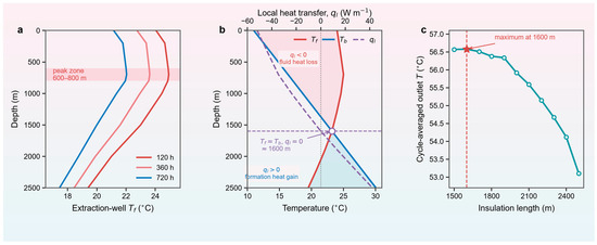
Figure 22 places the extraction-well fluid-temperature peak, the local heat-transfer crossover, and the insulation optimization on consistent depth and performance axes. The peak zone at 600–800 m and the crossover near 1600 m represent different physical definitions. The optimum results from the cycle-integrated balance between suppressing shallow heat loss and retaining deep heat gain; it is therefore reported as 1600 m only for the investigated geometry and conditions. A comparison with the principal related analytical models is provided in Table 9.

Figure 22. Relationship among the extraction-well fluid-temperature peak, local heat-transfer crossover, and insulation-length optimization. (a) Fluid-temperature profiles and the 600–800 m peak zone. (b) Fluid temperature, borehole-wall temperature, and local unit-length heat-transfer rate; $q_l$ changes sign near 1600 m. (c) Cycle-averaged outlet temperature for the investigated insulation lengths, with the discrete maximum at 1600 m.

Table 9. Comparison of the present framework with the principal related analytical models.

Model	Geometry	Seepage/Gradient	Stratification	Coupling/Insulation	Validation
Bao et al. [49]	Mid-deep UBHE	Included	Benchmark layers	Numerical benchmark	Primary benchmark
Jia et al. [45]	Butted horizontal wells	Included	Different layered mapping	Semi-analytical coupling	Related comparison
Luo et al. [39,40,41]	Deep coaxial borehole	Case-dependent	Segmented layers	Coaxial flow and insulation	Method reference
Present model	3-segment UBHE	Both included	Five equivalent layers	Segment-coupled FLS and extraction-well insulation	Bao and classical FLS

5. Conclusions

This study developed a segmented FLS analytical model for a mid-deep UBHE with geothermal gradient, layer-wise geological properties, groundwater seepage, and extraction-well insulation. The following conclusions are supported by the benchmark, limiting-case, convergence, and sensitivity analyses:

(1)

Against Bao et al. [49], the model gives an MAE of 0.87 °C, a maximum absolute error of 0.98 °C, and a mean relative error of 1.6%. The classical FLS limiting case gives an MAE of 0.012 °C and a maximum relative-error magnitude of 0.41%. The unsupported statement of a <$2.5\mathrm{\%}$ deviation from Jia et al. is removed.

(2)

The extraction-well fluid-temperature peak occurs at 600–800 m, while the local heat-transfer direction changes near 1600 m. For the investigated 2500–650–2500 m geometry, the maximum cycle-averaged outlet temperature occurs at an insulation length of 1600 m, corresponding to $L_{\mathrm{o}\mathrm{p}\mathrm{t}}/H=0.64$

(3)

Seepage increases the cycle-averaged outlet temperature with diminishing gains. Deep-layer conductivity enhances useful heat extraction, whereas shallow-layer conductivity increases reverse heat loss. Sensitivity to the geothermal gradient is greater than that to small variations in equivalent conductivity.

(4)

Increased volumetric heat capacity provides the greatest long-term thermal stability, with a ten-year drawdown of 1.10 °C and $SI=0.974$, compared with 1.89 °C and $SI=0.955$ for the baseline and 3.42 °C and $SI=0.920$ for the enhanced-conductivity case.

5.1. Limitations

The model uses cross-sectionally averaged one-dimensional fluid flow, neglects contact resistance and local U-bend effects, treats properties as constant within each layer, and represents interfaces through a layer-wise equivalent approximation. Long-range inter-well interference is neglected only for well spacing much larger than the thermal influence radius. The optimum 1600 m insulation length is specific to the investigated geometry, geology, and load. The classical FLS comparison is an analytical limiting-case verification and does not replace long-term field validation.

5.2. Engineering Implications

Design should prioritize the heat-supply capacity of deep strata while using extraction-well insulation to suppress shallow reverse heat loss. The insulation endpoint should be selected near the cycle-dependent depth at which the local net heat-transfer rate changes sign, rather than by transferring the absolute 1600 m value to another project. For each site, the insulation length must be re-optimized using the actual borehole depth, geothermal gradient, layer properties, seepage conditions, and operating load.

6. Patents

• Patent Title: Dynamic assessment method for deep geothermal energy
• Patent Number: ZL 2024 1 0694896.1

Appendix A.1. Coordinate Systems, Distance Functions, and Segment Ranges

Independent local coordinates $s_1$, $s_2$, and $s_3$ are used for the injection, horizontal, and extraction sections. Their source-point coordinates, vertical depths, and integration ranges are identical to those defined in Section 2.2.1.

Coordinates and ranges of each section:

$$n=1: s_1\in \left[0,H_1\right], {{\mathbf{X}}^{\prime }}_1=\left(0,0,s_1\right), z_1\left(s_1\right)=s_1$$

$$n=2: s_2\in \left[0,L_h\right], {{\mathbf{X}}^{\prime }}_2=\left(s_2,0,H_1\right), z_2\left(s_2\right)=H_1$$

$$n=3: s_3\in \left[0,H_3\right], {{\mathbf{X}}^{\prime }}_3=\left(L_h,0,H_1-s_3\right), z_3\left(s_3\right)=H_1-s_3$$

All real-source and image-source distances use the square root of the sum of squared coordinate differences, including the anisotropy ratios ${\kappa }_{zx}$ and ${\kappa }_{zy}$.

$$d_1={\left[{\kappa }_{zx}{x}^2+{\kappa }_{zy}{y}^2+{\left(z-s_1\right)}^2\right]}^{1/2}; d{\prime }_1={\left[{\kappa }_{zx}{x}^2+{\kappa }_{zy}{y}^2+{\left(z+s_1\right)}^2\right]}^{1/2}$$

$$d_2={\left[{\kappa }_{zx}{\left(x-s_2\right)}^2+{\kappa }_{zy}{y}^2+{\left(z-H_1\right)}^2\right]}^{1/2}; d{\prime }_2={\left[{\kappa }_{zx}{\left(x-s_2\right)}^2+{\kappa }_{zy}{y}^2+{\left(z+H_1\right)}^2\right]}^{1/2}$$

$$d_3={\left[{\kappa }_{zx}{\left(x-L_h\right)}^2+{\kappa }_{zy}{y}^2+{\left(z-H_1+s_3\right)}^2\right]}^{1/2}; d{\prime }_3={\left[{\kappa }_{zx}{\left(x-L_h\right)}^2+{\kappa }_{zy}{y}^2+{\left(z+H_1-s_3\right)}^2\right]}^{1/2}$$

The segment lengths are $L_1=H_1$, $L_2=L_h$, and $L_3=H_3$; no cumulative path coordinate is used as an integration limit.

Figure A1. Schematic diagram of the extended virtual heat source method. Reproduced from Ref. [46] under the Creative Commons Attribution (CC BY 4.0) license.

Figure A1. Schematic diagram of the extended virtual heat source method. Reproduced from Ref. [46] under the Creative Commons Attribution (CC BY 4.0) license.

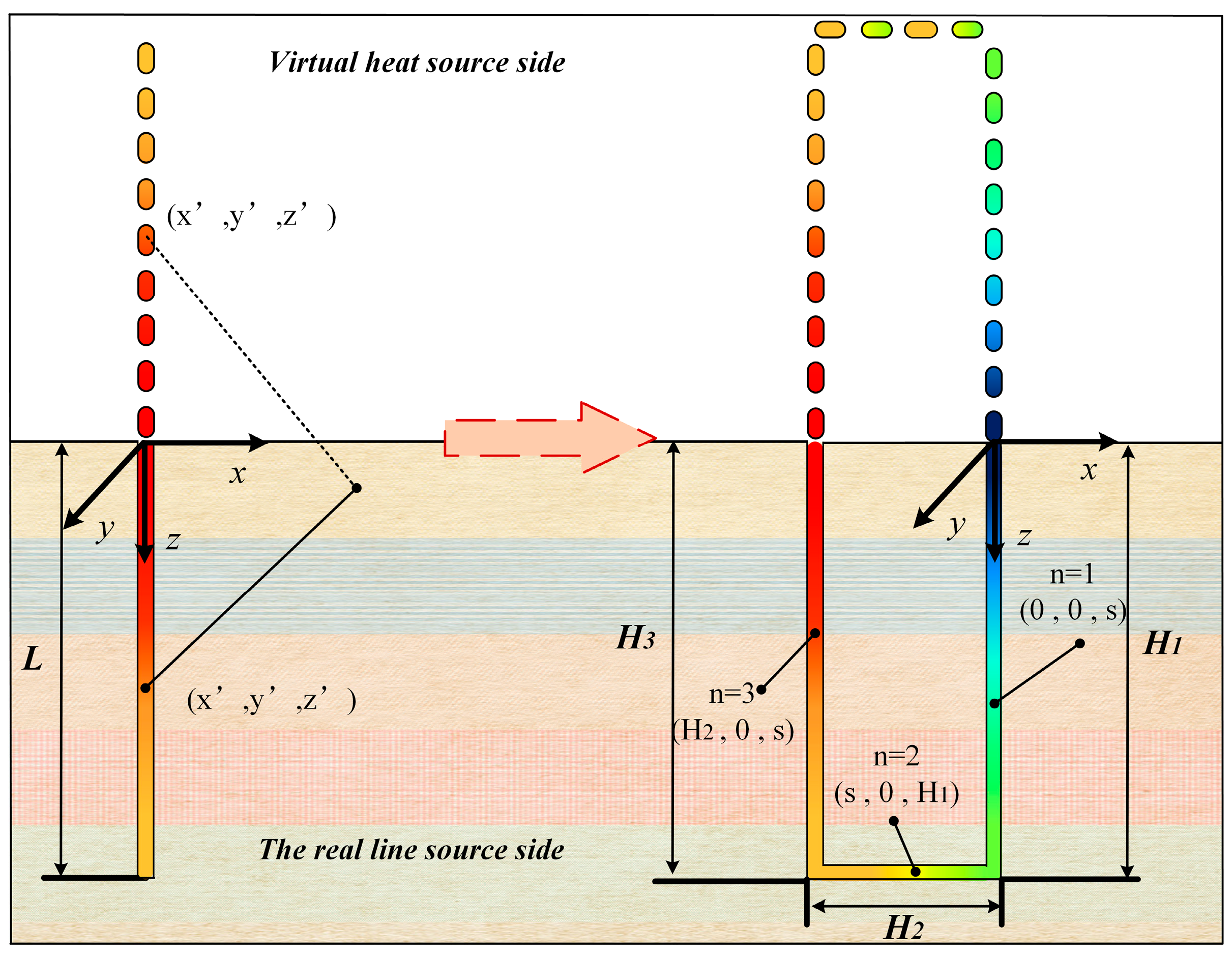
Substitution of the revised local coordinates and distance functions into Equation (6) gives the corrected segmented FLS temperature-field expression used in the main text.

Appendix A.2. Instantaneous Point-Source Kernel (Equation (A1))

Equation (A1) is the Green’s function of an instantaneous point source in an anisotropic medium [48].

$$\mathrm{G}(\mathrm{X},\mathrm{t};{\mathrm{X}}^{\prime },{\mathrm{t}}^{\prime })={\displaystyle \frac{[\mathsf{\rho }\mathrm{c}/(\mathrm{t}-{\mathrm{t}}^{\prime }){]}^{3/2}}{8{\mathsf{\pi }}^{3/2}\sqrt{{\mathrm{k}}_{\mathrm{x}}{\mathrm{k}}_{\mathrm{y}}{\mathrm{k}}_{\mathrm{z}}}}}\exp \{-{\displaystyle \frac{\mathsf{\rho }\mathrm{c}}{4(\mathrm{t}-{\mathrm{t}}^{\prime })}}[{\displaystyle \frac{(\mathrm{x}-{\mathrm{x}}^{\prime }{)}^2}{{\mathrm{k}}_{\mathrm{x}}}}+{\displaystyle \frac{(\mathrm{y}-{\mathrm{y}}^{\prime }{)}^2}{{\mathrm{k}}_{\mathrm{y}}}}+{\displaystyle \frac{(\mathrm{z}-{\mathrm{z}}^{\prime }{)}^2}{{\mathrm{k}}_{\mathrm{z}}}}]\}$$

(A1)

Appendix A.3. Continuous Heat Release (Equation (A2))

Integrating the point source over t′ = 0 → t gives the continuous point-source response of Equation (A2).

$${\mathsf{\theta }}_{\mathrm{p}}(\mathrm{X},\mathrm{t})={\displaystyle \frac{(\mathsf{\rho }\mathrm{c}/\mathsf{\pi }{)}^{3/2}}{8\sqrt{{\mathrm{k}}_{\mathrm{x}}{\mathrm{k}}_{\mathrm{y}}{\mathrm{k}}_{\mathrm{z}}}}}{\int }_0^{\mathrm{t}}{\displaystyle \frac{1}{(\mathrm{t}-{\mathrm{t}}^{\prime }{)}^{3/2}}}\mathrm{e}\mathrm{x}\mathrm{p}\{-{\displaystyle \frac{\mathsf{\rho }\mathrm{c}}{4(\mathrm{t}-{\mathrm{t}}^{\prime })}}[{\displaystyle \frac{(\mathrm{x}-{\mathrm{x}}^{\prime }{)}^2}{{\mathrm{k}}_{\mathrm{x}}}}+{\displaystyle \frac{(\mathrm{y}-{\mathrm{y}}^{\prime }{)}^2}{{\mathrm{k}}_{\mathrm{y}}}}+{\displaystyle \frac{(\mathrm{z}-{\mathrm{z}}^{\prime }{)}^2}{{\mathrm{k}}_{\mathrm{z}}}}]\}\mathrm{d}{\mathrm{t}}^{\prime }$$

(A2)

Appendix A.4. Error-Function Form (Equation (A3))

Using the combined distance variable d and thermal diffusivities αx, αy, and αz, Equation (A3) is obtained.

$${\mathsf{\theta }}_{\mathrm{p}}(\mathrm{X},\mathrm{t})={\displaystyle \frac{(\mathsf{\rho }\mathrm{c}/\mathsf{\pi }{)}^{3/2}}{4\sqrt{{\mathrm{k}}_{\mathrm{x}}{\mathrm{k}}_{\mathrm{y}}{\mathrm{k}}_{\mathrm{z}}}}}{\int }_{1/\sqrt{\mathrm{t}}}^{\mathrm{\infty }}\mathrm{e}\mathrm{x}\mathrm{p}(-{\displaystyle \frac{{\mathrm{d}}^2{\mathsf{\tau }}^2}{4{\mathsf{\alpha }}_{\mathrm{z}}}})\mathrm{d}\mathsf{\tau }={\displaystyle \frac{1}{4\mathsf{\pi }\mathrm{d}\sqrt{{\mathsf{\alpha }}_{\mathrm{x}}{\mathsf{\alpha }}_{\mathrm{y}}}}}\mathrm{e}\mathrm{r}\mathrm{f}\mathrm{c}({\displaystyle \frac{\mathrm{d}}{2\sqrt{{\mathsf{\alpha }}_{\mathrm{z}}\mathrm{t}}}})$$

(A3)

Appendix A.5. Finite Line Source (Equation (A4))

Integrating the point-source solution along a finite line of length L yields Equation (A4).

$$\mathsf{\theta }(\mathrm{z},\mathrm{t})={\displaystyle \frac{{\mathrm{q}}_{\mathrm{l}}}{4\mathsf{\pi }\sqrt{{\mathrm{k}}_{\mathrm{x}}{\mathrm{k}}_{\mathrm{y}}}}}{\int }_0^{\mathrm{L}}{\displaystyle \frac{1}{\mathrm{d}}}\mathrm{e}\mathrm{r}\mathrm{f}\mathrm{c}({\displaystyle \frac{\mathrm{d}}{2\sqrt{{\mathsf{\alpha }}_{\mathrm{z}}\mathrm{t}}}})\mathrm{d}{\mathrm{z}}^{\prime }$$

(A4)

Appendix A.6. Virtual Image Method (Equation (A5))

The opposite-sign mirror source at the reflected vertical coordinate enforces zero temperature perturbation at $z=0$, and therefore the Dirichlet surface condition used in the main model.

$${\mathsf{\theta }}^{\prime }(\mathrm{z},\mathrm{t})=-{\displaystyle \frac{{\mathrm{q}}_{\mathrm{l}}}{4\mathsf{\pi }\sqrt{{\mathrm{k}}_{\mathrm{x}}{\mathrm{k}}_{\mathrm{y}}}}}{\int }_0^{\mathrm{L}}{\displaystyle \frac{1}{{\mathrm{d}}^{\prime }}}\mathrm{e}\mathrm{r}\mathrm{f}\mathrm{c}({\displaystyle \frac{{\mathrm{d}}^{\prime }}{2\sqrt{{\mathsf{\alpha }}_{\mathrm{z}}\mathrm{t}}}})\mathrm{d}{\mathrm{z}}^{\prime }$$

(A5)

Appendix A.7. Composite FLS Solution (Equation (A6))

Superposition of the real and opposite-sign image sources produces Equation (A6).

$${\mathsf{\theta }}_{\mathrm{f}\mathrm{l}\mathrm{s}}(\mathrm{z},\mathrm{t})=\mathsf{\theta }+{\mathsf{\theta }}^{\prime }={\displaystyle \frac{{\mathrm{q}}_{\mathrm{l}}}{4\mathsf{\pi }\sqrt{{\mathrm{k}}_{\mathrm{x}}{\mathrm{k}}_{\mathrm{y}}}}}{\int }_0^{\mathrm{L}}[{\displaystyle \frac{\mathrm{e}\mathrm{r}\mathrm{f}\mathrm{c}(\mathrm{d}/2\sqrt{{\mathsf{\alpha }}_{\mathrm{z}}\mathrm{t}})}{\mathrm{d}}}-{\displaystyle \frac{\mathrm{e}\mathrm{r}\mathrm{f}\mathrm{c}({\mathrm{d}}^{\prime }/2\sqrt{{\mathsf{\alpha }}_{\mathrm{z}}\mathrm{t})}}{{\mathrm{d}}^{\prime }}}]\mathrm{d}{\mathrm{z}}^{\prime }$$

(A6)

Appendix A.8. Segmented UBHE Superposition (Equation (A7))

Substituting the three independent local-coordinate systems into Equation (A6) and using $q_l\left(s_n,t\right)$ gives the segmented UBHE superposition in Equation (A7).

$$T_b\left(\mathbf{X},t\right)={\displaystyle \sum _{n=1}^3}{\displaystyle \frac{q_l\left(s_n,t\right)}{4\pi \sqrt{k_{x,n}{k}_{y,n}}}}{\int }_0^{L_n}\left[{\displaystyle \frac{\mathrm{e}\mathrm{r}\mathrm{f}\mathrm{c}\left(d_n/\left(2\sqrt{{\alpha }_{z,n}t}\right)\right)}{d_n}}-{\displaystyle \frac{\mathrm{e}\mathrm{r}\mathrm{f}\mathrm{c}\left({d^{\prime }}_n/\left(2\sqrt{{\alpha }_{z,n}t}\right)\right)}{{d^{\prime }}_n}}\right]d{s}_n$$

(A7)

Appendix A.9. Layer-Wise Equivalent Properties in Equation (A7)

For each integration element, $k_{\mathrm{e}\mathrm{q}\mathrm{u}}$ and ${\alpha }_{\mathrm{e}\mathrm{q}\mathrm{u}}$ are evaluated from Equations (9) and (10) using the properties of the layer containing that element. When an integration path crosses an interface, it is divided into layer-specific subintervals. This is a layer-wise equivalent approximation rather than an explicit local interface solution.

Appendix A.10. Surface Boundary Verification After Superposition

Because every real segment is paired with an opposite-sign image segment, the temperature perturbation cancels at $z=0$ for the complete three-segment superposition, satisfying the prescribed Dirichlet boundary.

Appendix A.11. Coupling to Equations (8)–(11)

Equation (A7) provides $T_b\left(s,t\right)$, Equation (8) defines $q_l\left(s,t\right)$ through the unit-length resistance $R^{\prime }$, and Equation (11) governs the segment-wise fluid temperature. Iteration continues until $\mathrm{m}\mathrm{a}\mathrm{x}\left|T^k-T^{k-1}\right|<{10}^{-4}$ °C.

References

- Lee, I.; Tester, J.W.; You, F. Systems analysis, design, and optimization of geothermal energy systems for power production and polygeneration: State-of-the-art and future challenges. JUL Renew. Sustain. Energy Rev. 2019, 109, 551–577. [Google Scholar] [CrossRef] [Scilit]
- Menéndez, J.; Ordóñez, A.; Álvarez, R.; Loredo, J. Energy from closed mines: Underground energy storage and geothermal applications. JUL Renew. Sustain. Energy Rev. 2019, 108, 498–512. [Google Scholar] [CrossRef] [Scilit]
- El Haj Assad, M.; Ahmadi, M.H.; Sadeghzadeh, M.; Yassin, A.; Issakhov, A. Renewable hybrid energy systems using geothermal energy: Hybrid solar thermal-geothermal power plant. Int. J. Low Carbon Technol. 2021, 16, 518–530. [Google Scholar] [CrossRef] [Scilit]
- Moya, D.; Aldas, C.; Kaparaju, P. Geothermal energy: Power plant technology and direct heat applications. OCT Renew. Sustain. Energy Rev. 2018, 94, 889–901. [Google Scholar] [CrossRef] [Scilit]
- Okoroafor, E.R.; Smith, C.M.; Ochie, K.I.; Nwosu, C.J.; Gudmundsdottir, H.; Aljubran, M.J. Machine learning in subsurface geothermal energy: Two decades in review. Geothermics 2022, 102, 102401. [Google Scholar] [CrossRef] [Scilit]
- Olasolo, P.; Juárez, M.C.; Morales, M.P.; Liarte, I.A. Enhanced geothermal systems (EGS): A review. Renew. Sustain. Energy Rev. 2016, 56, 133–144. [Google Scholar] [CrossRef] [Scilit]
- Bayer, P.; Saner, D.; Bolay, S.; Rybach, L.; Blum, P. Greenhouse gas emission savings of ground source heat pump systems in Europe: A review. Renew. Sustain. Energy Rev. 2012, 16, 1256–1267. [Google Scholar] [CrossRef] [Scilit]
- Cunha, R.P.; Bourne-Webb, P.J. A critical review on the current knowledge of geothermal energy piles to sustainably climatize buildings. Renew. Sustain. Energy Rev. 2022, 158, 112072. [Google Scholar] [CrossRef] [Scilit]
- Cai, W.; Wang, F.; Liu, J.; Wang, Z.; Ma, Z. Experimental and numerical investigation of heat transfer performance and sustainability of deep borehole heat exchangers coupled with ground source heat pump systems. Appl. Therm. Eng. 2018, 149, 975–986. [Google Scholar] [CrossRef] [Scilit]
- Nian, Y.-L.; Cheng, W.-L.; Yang, X.-Y.; Xie, K. Simulation of a novel deep ground source heat pump system using abandoned oil wells with coaxial BHE. Int. J. Heat Mass Tran. 2019, 137, 400–412. [Google Scholar] [CrossRef] [Scilit]
- Zhang, W.; Li, W.; Sørensen, B.R.; Cui, P.; Man, Y.; Yu, M.; Fang, Z. Comparative analysis of heat transfer performance of coaxial pipe and U-type deep borehole heat exchangers. J. Geotherm. 2021, 96, 102220. [Google Scholar] [CrossRef] [Scilit]
- Zhang, W.; Wang, J.; Zhang, F.; Lu, W.; Cui, P.; Guan, C.; Fang, Z. Heat transfer analysis of U-type deep borehole heat exchangers of geothermal energy. Energy Build. 2021, 237, 110794. [Google Scholar] [CrossRef] [Scilit]
- Kang, W.K.; Liu, F.; Yang, F.F.; Wang, H.J. Simulation of heat transfer performance using middle-deep coaxial borehole heat exchangers by FEFLOW. J. Groundw. Sci. Eng. 2020, 8, 315–327. [Google Scholar]
- Li, C.; Guan, Y.; Jiang, C.; Deng, S.; Lu, Z. Numerical study on the heat transfer, extraction, and storage in a deep-buried pipe. Renew. Energy 2020, 152, 1055–1066. [Google Scholar] [CrossRef] [Scilit]
- Li, C.; Guan, Y.; Wang, X. Study on reasonable selection of insulation depth of the outlet section of vertical deep-buried U-bend tube heat exchanger. Energy Build. 2018, 167, 231–239. [Google Scholar] [CrossRef] [Scilit]
- Li, J.; Xu, W.; Li, J.; Huang, S.; Li, Z.; Qiao, B.; Yang, C.; Sun, D.; Zhang, G. Heat extraction model and characteristics of coaxial deep borehole heat exchanger. Renew. Energy 2021, 169, 738–751. [Google Scholar] [CrossRef] [Scilit]
- Brown, C.S.; Cassidy, N.J.; Egan, S.S.; Griffiths, D. Numerical modelling of deep coaxial borehole heat exchangers in the Cheshire Basin, UK. Comput. Geosci. 2021, 152, 104752. [Google Scholar] [CrossRef] [Scilit]
- Huang, Y.; Zhang, Y.; Xie, Y.; Zhang, Y.; Gao, X. Thermal performance analysis on the composition attributes of deep coaxial borehole heat exchanger for building heating. Energy Build. 2020, 221, 110019. [Google Scholar] [CrossRef] [Scilit]
- Fang, L.; Diao, N.; Shao, Z.; Zhu, K.; Fang, Z. A computationally efficient numerical model for heat transfer simulation of deep borehole heat exchangers. Energy Build. 2018, 167, 79–88. [Google Scholar] [CrossRef] [Scilit]
- Huang, X.; Yao, Z.; Cai, H.; Li, X.; Chen, H. Performance evaluation of coaxial borehole heat exchangers considering ground non-uniformity based on analytical solutions. Int. J. Therm. Sci. 2021, 170, 107162. [Google Scholar] [CrossRef] [Scilit]
- Jiao, K.; Sun, C.; Yang, R.; Yu, B.; Bai, B. Long-term heat transfer analysis of deep coaxial borehole heat exchangers via an improved analytical model. Appl. Therm. Eng. 2021, 197, 117370. [Google Scholar] [CrossRef] [Scilit]
- Liu, J.; Wang, F.; Cai, W.; Wang, Z.; Li, C. Numerical investigation on the effects of geological parameters and layered subsurface on the thermal performance of mediumdeep borehole heat exchanger. Renew. Energy 2020, 149, 384–399. [Google Scholar] [CrossRef] [Scilit]
- Deng, J.; Wei, Q.; He, S.; Liang, M.; Zhang, H. Simulation analysis on the heat performance of deep borehole heat exchangers in medium-depth geothermal heat pump systems. Energies 2020, 13, 754. [Google Scholar] [CrossRef] [Scilit]
- Huang, Y.; Zhang, Y.; Xie, Y.; Zhang, Y.; Gao, X.; Ma, J. Field test and numerical investigation on deep coaxial borehole heat exchanger based on distributed optical fiber temperature sensor. Energy 2020, 210, 118643. [Google Scholar] [CrossRef] [Scilit]
- Li, C.; Guan, Y.; Liu, J.; Jiang, C.; Yang, R.; Hou, X. Heat Transfer Performance of a Deep Ground Heat Exchanger for Building Heating in Long-Term Service. Renew. Energy 2020, 166, 20–34. [Google Scholar] [CrossRef] [Scilit]
- Jiao, K.; Yang, R.; Sun, C.; Yu, B.; Bai, B. Stratum temperature recovery considering groundwater advection in periodic operations of deep borehole heat exchangers. Appl. Therm. Eng. 2022, 206, 118113. [Google Scholar] [CrossRef] [Scilit]
- Hu, X.; Banks, J.; Guo, Y.; Huang, G.; Liu, W.V. Effects of temperature-dependent property variations on the output capacity prediction of a deep coaxial borehole heat exchanger. Renew. Energy 2021, 165, 334–349. [Google Scholar] [CrossRef] [Scilit]
- Hecht-Méndez, J.; de Paly, M.; Beck, M.; Bayer, P. Optimization of energy extraction for vertical closed-loop geothermal systems considering groundwater flow. Energy Convers. Manag. 2013, 66, 1–10. [Google Scholar] [CrossRef] [Scilit]
- Wagner, V.; Blum, P.; Kübert, M.; Bayer, P. Analytical approach to groundwater-influenced thermal response tests of grouted borehole heat exchangers. Geothermics 2013, 46, 22–31. [Google Scholar] [CrossRef] [Scilit]
- Carslaw, H.S.; Jaeger, J.C.; Feshbach, H. Conduction of heat in solids. Phys. Today 2009, 15, 74–76. [Google Scholar] [CrossRef] [Scilit][Green Version]
- Eskilson, P. Thermal Analysis of Heat Extraction Boreholes. Doctoral Dissertation, University of Lund, Lund, Sweden, 1987. [Google Scholar]
- Diao, N.; Li, Q.; Fang, Z. Heat transfer in ground heat exchangers with groundwater advection. Int. J. Therm. Sci. 2004, 43, 1203–1211. [Google Scholar] [CrossRef] [Scilit]
- Meng, X.; Han, Z.; Hu, H.; Zhang, H.; Li, X. Studies on the performance of ground source heat pump affected by soil freezing under groundwater seepage. J. Build. Eng. 2021, 33, 101632. [Google Scholar] [CrossRef] [Scilit]
- Tolooiyan, A.; Hemmingway, P. A preliminary study of the effect of groundwater flow on the thermal front created by borehole heat exchangers. Int. J. Low Carbon Technol. 2014, 9, 284–295. [Google Scholar] [CrossRef] [Scilit]
- Wang, H.; Qi, C.; Du, H.; Gu, J. Thermal performance of borehole heat exchanger under groundwater flow: A case study from Baoding. Energy Build. 2009, 41, 1368–1373. [Google Scholar] [CrossRef] [Scilit]
- Fan, R.; Jiang, Y.; Yao, Y.; Shiming, D.; Ma, Z. A study on the performance of a geothermal heat exchanger under coupled heat conduction and groundwater advection. Energy 2007, 32, 2199–2209. [Google Scholar] [CrossRef] [Scilit]
- Pan, A.; Lu, L.; Cui, P.; Jia, L. A new analytical heat transfer model for deep borehole heat exchangers with coaxial tubes. Int. J. Heat Mass Tran. 2019, 141, 1056–1065. [Google Scholar] [CrossRef] [Scilit]
- Wang, C.; Lu, Y.; Chen, L.; Huang, Z.; Fang, H. A semi-analytical model for heat transfer in coaxial borehole heat exchangers. J. Geotherm. 2021, 89, 101952. [Google Scholar] [CrossRef] [Scilit]
- Luo, Y.; Guo, H.; Meggers, F.; Zhang, L. Deep coaxial borehole heat exchanger: Analytical modeling and thermal analysis. Energy 2019, 185, 1298–1313. [Google Scholar] [CrossRef] [Scilit]
- Luo, Y.; Yu, J.; Yan, T.; Zhang, L.; Liu, X. Improved analytical modeling and system performance evaluation of deep coaxial borehole heat exchanger with segmented finite cylinder-source method. Energy Build. 2020, 212, 109829. [Google Scholar] [CrossRef] [Scilit]
- Luo, Y.; Xu, G.; Yan, T. Performance evaluation and optimization design of deep ground source heat pump with non-uniform internal insulation based on analytical solutions—ScienceDirect. Energy Build. 2020, 229, 110495. [Google Scholar] [CrossRef] [Scilit]
- Luo, Y.; Xu, G.; Cheng, N. Proposing stratified segmented finite line source (SS-FLS) method for dynamic simulation of medium-deep coaxial borehole heat exchanger in multiple ground layers. Renew. Energy 2021, 179, 604–624. [Google Scholar] [CrossRef] [Scilit]
- Pan, S.; Kong, Y.; Chen, C.; Pang, Z.; Wang, J. Optimization of the utilization of deep borehole heat exchangers. Geoth. Energy 2020, 8, 6. [Google Scholar] [CrossRef] [Scilit]
- Zhao, Y.; Ma, Z.; Pang, Z. A fast simulation approach to the thermal recovery characteristics of deep borehole heat exchanger after heat extraction. Sustainability 2020, 12, 2021. [Google Scholar] [CrossRef] [Scilit]
- Jia, G.; Ma, Z.; Xia, Z.; Wang, J.; Zhang, Y.; Jin, L. Investigation of the horizontally-butted borehole heat exchanger based on a semi-analytical method considering groundwater seepage and geothermal gradient. Renew. Energy 2021, 171, 447–461. [Google Scholar] [CrossRef] [Scilit]
- Shi, Z.; Zhang, L.; He, P.; Xia, S.; Wang, C. An Analytical Investigation of the Heat-Transfer Performance of a Deep U-Shaped Borehole Heat-Exchangers System in Porous Media. Energies 2026, 19, 1353. [Google Scholar] [CrossRef] [Scilit]
- Li, M.; Lai, A.C. Heat-source solutions to heat conduction in anisotropic media with application to pile and borehole ground heat exchangers. Appl. Energy 2012, 96, 451–458. [Google Scholar] [CrossRef] [Scilit]
- Carslaw, H.S.; Jaeger, J.C. Conduction of Heat in SolidS. In SFPE Handbook of Fire Protection Engineering; Springer: New York, NY, USA, 1959; Volume 36, pp. 142–143. [Google Scholar] [CrossRef] [Scilit]
- Bao, L.; Wang, X.; Jin, P.; Cui, J.; Zhu, Y.; Wang, Y. An analytical heat transfer model for the mid-deep U-shaped borehole heat exchanger considering groundwater seepage. J. Build. Eng. 2023, 64, 105612. [Google Scholar] [CrossRef] [Scilit]
- Liu, Y.; Liu, B.; Zhu, H.; Lin, T.; Huo, Q.; Xing, J.; Li, S. Distribution Characteristics and Main Controlling Factors of Present-day Geothermal Field in Songliao Basin. Acta Geol. Sin. 2023, 97, 2715–2727. [Google Scholar] [CrossRef]
- Yuan, Y.; Zhu, W.; Mi, L.; Zhang, G.; Hu, S.; He, L. Uniform geothermal gradient" and heat flow in the Qiongdongnan and Pearl River Mouth Basins of the South China Sea. Mar. Pet. Geol. 2009, 26, 1152–1162. [Google Scholar] [CrossRef] [Scilit]
Disclaimer/Publisher’s Note: The statements, opinions and data contained in all publications are solely those of the individual author(s) and contributor(s) and not of MDPI and/or the editor(s). MDPI and/or the editor(s) disclaim responsibility for any injury to people or property resulting from any ideas, methods, instructions or products referred to in the content. |
© 2026 by the authors. Licensee MDPI, Basel, Switzerland. This article is an open access article distributed under the terms and conditions of the Creative Commons Attribution (CC BY) license.