


Abstract
Coherent vortices alter flapping-foil energy harvesting, but wake-generated vortex properties and timing are coupled to upstream-body kinematics. We use two-dimensional immersed boundary–lattice Boltzmann simulations of a prescribed heaving–pitching NACA0015 foil at . An independently prescribed Taylor vortex allows nominal encounter phase, body-fixed offset, diameter, and intensity to be varied at fixed kinematics. Production-grid is within of the fine-grid result; the fine-grid diffusion test gives a maximum full-field velocity error of against the analytical solution over . For the reference vortex with a pivot-centered nominal target (), nominal-encounter-aligned mean power coefficients of , , and occur at , , and , respectively, compared with without gusts. These define the power-reducing (PR), near-baseline (NB), and power-enhancing (PE) cases. Within the sampled ranges, diameter is associated mainly with disturbance reach and duration, intensity with loading magnitude, and offset with spatial overlap and interaction timing. Power variations are consistent with the timing of vortex-modified loading relative to prescribed foil motion. In three same-sign, once-per-cycle sequences, the PR–NB–PE ordering persists despite residual-wake interactions, with sustained mean power coefficients of , , and , respectively. Nominal encounter phase and foil placement should be considered jointly for repeatable or predictable vortex passages.
1. Introduction
Oscillating foils have been investigated as alternatives to rotary turbines for harvesting energy from wind, river, tidal, and ocean currents [1,2]. These devices convert fluid kinetic energy into mechanical work through prescribed or flow-induced heaving and pitching [3,4,5]. Under combined heaving and pitching, the instantaneous hydrodynamic power is given by the work rates of the force and pitching moment. Large loads alone do not guarantee positive energy extraction. Their timing relative to the translational and angular velocities is equally important. Leading- and trailing-edge vortices alter this timing by changing the surface-pressure distribution and, in turn, the force and moment histories [6].
The early Wingmill employed harmonically prescribed translation and pitching with a fixed phase relation and demonstrated the feasibility of oscillating-foil power extraction [3]. Subsequent studies examined the influence of pitching amplitude, heaving amplitude, reduced frequency, phase difference, pivot location, wake structure, and structural response [7,8,9,10,11]. Recent reviews summarize how foil kinematics, geometry, structural response, and inflow conditions affect energy-harvesting performance [12,13].
In practical oscillating-foil harvesters, the heaving and pitching degrees of freedom are coupled to a power-take-off system. The motion may be prescribed mechanically, maintained by active control, or generated passively through the balance among hydrodynamic loading, inertia, elastic restoring forces, and damping [4,5,10].
Transient or irregular inflow changes the magnitude and timing of the hydrodynamic loading. In a prescribed-motion device, this mainly alters the power transferred to the foil. A passive device may also undergo changes in oscillation amplitude, frequency, phase, or stability. Practical operation depends on maintaining stable motion and favorable load–velocity phasing without exceeding structural or power-take-off limits.
A substantial part of the existing literature has considered nominally uniform incoming flows. In practical environments, however, a harvesting device may encounter localized disturbances generated by upstream wakes, coherent vortical structures, or turbulent fluctuations [14]. Vortical gusts are especially relevant when their velocity and length scales are comparable to those of the foil [15]. Unlike a spatially uniform transverse gust, a localized vortex produces a non-uniform induced-velocity field that evolves as the vortex approaches, interacts with, and passes the foil.
The induced cross-stream velocity changes the effective angle of attack. Interaction between the incident vortex and foil-generated vorticity can also reorganize the separated flow. This interaction alters leading-edge-vortex development and wake shedding, with corresponding changes in the surface-pressure distribution [16,17]. The load history is set by the vortex structure together with the geometry and timing of the encounter.
Vortical-gust interactions with stationary or fixed-angle airfoils have been examined experimentally and numerically over a range of flow conditions. Barnes and Visbal [18,19] documented pronounced transient changes in aerodynamic loading and boundary-layer behavior at transitional Reynolds numbers.
At , Martínez-Muriel and Flores [17] examined Taylor vortices with different diameters, intensities, and vertical offsets relative to a NACA0012 airfoil. The time to the peak lift increment scaled with . Its magnitude was approximately proportional to vortex circulation, but varied nonlinearly with vortex–airfoil separation.
Qian et al. [20] further showed experimentally that a nearly two-dimensional incident vortex may deform, diffuse, and lose coherence while inducing leading-edge-vortex formation and shedding from the downstream wing. Recent high-fidelity studies also show that transient loading is sensitive to vortex strength, core size, initial position, and airfoil geometry [21,22].
These studies clarify how vortex properties and encounter geometry shape transient aerodynamic loading. Their target airfoils, however, are stationary or held at fixed incidence. The results do not establish whether the same loading would perform positive or negative work on an oscillating energy-harvesting foil.
Studies of tandem and wake-coupled oscillating foils directly address moving bodies and power extraction. Experiments show that downstream efficiency depends strongly on inter-foil phase [23]. Recent models relate the time-dependent power to the incident wake and foil kinematics [24]. Other experiments have identified kinematics that either avoid or exploit coherent wake vortices [25]. Ren et al. [26] classified constructive and destructive vortex–foil interactions according to vortex rotation and encounter side. In these upstream-wake configurations, the upstream-foil kinematics and array geometry determine the vortex scale, strength, trajectory, and arrival time. Changing one design parameter can modify several wake properties at once. Their individual energetic effects are then difficult to isolate. Repeatable vortical forcing has been demonstrated experimentally. Rockwood and Medina [27] controlled the frequency, strength, and transverse position of periodically generated vortices. Oshkai et al. [28] examined a fully passive turbine under periodically perturbed inflow. Beneficial forcing occurred only over a limited range of disturbance frequencies and upstream-foil motions. Together, these experiments establish the feasibility of synchronized vortex encounters. In an energy-harvesting arrangement, however, the disturbance characteristics remain tied to the upstream generating system.
Together, these studies leave two related questions unresolved. With the foil kinematics fixed, the individual effects of encounter phase, body-fixed offset, vortex diameter, and vortex intensity on the power change relative to uniform inflow remain unclear. It is also unknown whether the phase ordering identified for an isolated encounter persists under repeated encounters.
We investigate a two-dimensional NACA0015 foil undergoing prescribed heaving and pitching at using an immersed boundary–lattice Boltzmann method. The Taylor vortex is introduced independently of an upstream body, and its nominal encounter is referenced to the pitching pivot in an instantaneous foil-fixed frame. This formulation allows encounter phase, body-fixed offset, vortex diameter, and vortex intensity to be varied without changing the foil kinematics.
The phase response is quantified by the mean power over the complete cycle beginning at the nominal encounter time. Three representative cases are retained for further analysis: power-reducing (PR), near-baseline (NB), and power-enhancing (PE). They provide the basis for examining vortex diameter, vortex intensity, and body-fixed offset. Repeated same-sign encounters test whether the isolated-event phase ordering survives in the presence of wake memory. By decoupling the prescribed vortex variables from upstream-wake generation, the framework provides a common basis for controlled comparisons of isolated and repeated encounters. The two-dimensional prescribed-motion model is used to examine phase-conditioned associations between gust-modified loading and hydrodynamic power. Its application scope and limitations are discussed in Section 4.4.
Section 2 defines the physical problem and performance metrics. Section 3 presents the numerical formulation. The computational setup and numerical verification are documented in Appendix A. Section 4 examines the phase and parameter responses to isolated encounters before turning to repeated encounters and flow-field interpretations. The main conclusions are summarized in Section 5.
2. Physical Problem
2.1. Foil Kinematics and Baseline Condition
In this study, a two-dimensional NACA0015 foil undergoing prescribed heaving and pitching motions is considered for energy harvesting. The foil kinematics are defined as
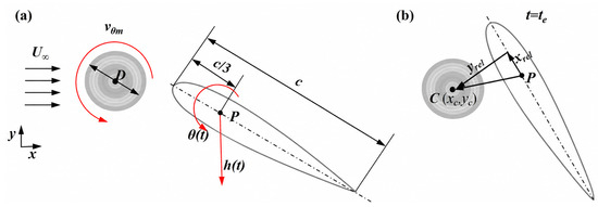
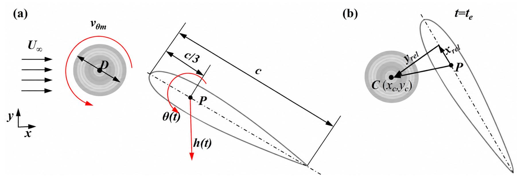
where and are the pitching and heaving amplitudes, respectively, f is the flapping frequency, and is the phase difference between the two motions. As shown in Figure 1a, the pitching pivot is located at from the leading edge, where c denotes the chord length. A uniform freestream of velocity is imposed at the inlet.
Figure 1.
Schematic of the physical problem and gust–foil encounter definition: (a) prescribed heaving–pitching motion of the NACA0015 foil subjected to an incoming Taylor vortex and (b) instantaneous body-fixed coordinate system and scheduled nominal vortex-center target at . A nonzero body-fixed offset is shown for clarity.
Unless otherwise stated, the baseline parameters are , °, °, , and . This parameter set matches the high-efficiency reference condition of Kinsey and Dumas [7], who reported using a swept-area normalization. The same kinematics have also been adopted in related flapping-foil studies [29,30]. These kinematics are retained to provide a fixed reference for evaluating the effects of the prescribed vortex encounters.
The geometric pitching amplitude should be interpreted together with the heaving velocity. For °, the nominal kinematic effective angle in uniform inflow is
Here, , giving a maximum heave-induced relative-flow angle of °. The combined kinematics yield °, even though the geometric pitching amplitude is °.
The choice preserves direct comparability with the reference condition. It also confines the present analysis to a controlled, two-dimensional low-Reynolds-number regime. Dimensional operating conditions follow from
For reference, in water with and , the present condition corresponds to , , and , representing one laboratory-scale realization rather than a unique full-scale operating point.
2.2. Taylor-Vortex Model and Encounter Definition
The incoming disturbance is modeled as a finite-core Taylor vortex introduced upstream of the moving foil.
The vortex is characterized by a diameter D and a circumferential-velocity scale . Its tangential velocity profile is
where
is the distance from to the vortex center .
Under the coordinate convention in Figure 1, defines a clockwise vortex. The profile reaches
The parameter represents a characteristic velocity scale. The actual peak tangential speed is . Following Martínez-Muriel and Flores [17], we use and as the nondimensional vortex diameter and vortex intensity, respectively.
Because the foil heaves and pitches simultaneously, the gust–foil encounter is defined in an instantaneous body-fixed coordinate system attached to the pitching pivot, as shown in Figure 1b. The nominal encounter time is written as
where , is the number of completed periods preceding the nominal encounter time, and is the fractional encounter phase. At , the scheduled vortex-center target is specified relative to the pitching pivot by the body-fixed coordinates , representing chordwise and normal offsets, respectively.
The parameter specifies the foil kinematic state at the scheduled encounter. It can be varied without changing the vortex diameter, vortex intensity, or body-fixed offset.
The global coordinate origin is placed at the mean pitching-pivot position, with the x- and y-axes aligned with the streamwise and transverse directions, respectively. Since the pivot has no prescribed streamwise translation, its position at is . The scheduled target in the global frame is therefore
The vortex is introduced at the upstream plane
and the nominal injection time is estimated from
Equation (11) determines only the time of the one-time vortex insertion. It does not prescribe the subsequent vortex-center trajectory. Nor does it force the evolved vortex center to coincide exactly with the scheduled target at . After insertion, the vortex convects and diffuses under the multiple-relaxation-time lattice Boltzmann method (MRT–LBM) evolution. Its shape and trajectory may then change through interaction with the moving foil. The population-level update is given in Section 3.1.2.
Figure 1 separates the fixed foil kinematics from four controlled encounter variables: , , , and . The transformation to the global frame provides a common geometric definition for encounters scheduled at different foil attitudes. These variables specify the nominal encounter target at . They do not prescribe the vortex trajectory after insertion.
2.3. Energy-Harvesting Metrics
Energy-harvesting performance is evaluated from the hydrodynamic power transferred from the flow to the prescribed foil motion. Let denote the Lagrangian force per unit arc length exerted by the foil on the fluid, and let denote the prescribed boundary velocity. The instantaneous extracted power per unit span and its chord-normalized coefficient are
The boundary integral is the rate at which the foil does work on the fluid. The minus sign reverses this convention. With the present definition, denotes power transferred from the fluid to the foil. The denominator is based on the conventional projected reference area for unit span. is a power coefficient, not a conversion efficiency. Values above unity are admissible under this normalization.
The global transverse force and pitching moment exerted by the fluid on the foil are
where is the boundary position and is the pitching-pivot position. The lift coefficient is
Here, is resolved along the fixed global y-direction, not along the normal to the instantaneous foil chord.
For a rigid foil with no prescribed streamwise translation,
The pitching pivot has no prescribed streamwise translation, so and the term vanishes. A drag coefficient is not introduced as a separate energy-harvesting metric. The effect of streamwise loading remains included through its contribution to . This heave–pitch decomposition and chord-based reference power are commonly used in oscillating-foil energy-harvesting studies [7,26].
The response to an isolated encounter is quantified by the mean power coefficient over one complete foil-motion cycle beginning at the nominal encounter time,
This fixed-window mean is intended for phase-conditioned comparison; it does not quantify the net energy difference from the no-gust baseline over the full isolated-encounter transient.
Because is a prescribed geometric and phase reference rather than an observed vortex-center passage time, the interval is hereafter termed the nominal-encounter-aligned cycle. The no-gust baseline is averaged over the same phase-aligned interval. The averaging interval for repeated encounters is defined in Section 4.3.
The corresponding swept-height-normalized hydrodynamic efficiency is
where d is the peak-to-peak transverse excursion of the trailing edge. With the pivot located at from the leading edge,
and
For the prescribed kinematics, . For unit span, the corresponding swept frontal area is . This normalization follows conventional oscillating-foil practice [7,26,30,31].
Because is fixed by the prescribed kinematics, and give identical case rankings and relative percentage changes. Both are hydrodynamic performance measures and exclude power-take-off, mechanical-transmission, and electrical-conversion losses.
3. Numerical Methods
3.1. Lattice Boltzmann Method for the Fluid Flow
3.1.1. MRT–LBM Formulation
The flow is solved using a two-dimensional nine-velocity (D2Q9) lattice Boltzmann method (LBM) within the multiple-relaxation-time (MRT) framework [32,33]. The evolution of the distribution function associated with the discrete velocity is
where is the time step and and denote the MRT collision and forcing contributions, respectively. The collision term is
where M is the D2Q9 transformation matrix and S is the diagonal relaxation matrix.
The MRT forcing contribution is written as
Here, denotes the discrete representation of the Eulerian immersed-boundary force density [33,34]. The macroscopic density and momentum are recovered from
The equilibrium distribution and the discrete forcing term are
Here, is the lattice weight, and the lattice sound speed is .
The kinematic viscosity is set by the relaxation rate of the shear modes,
The present calculations are two-dimensional and laminar at . No transition or turbulence model is used. Spatial refinement follows the multi-block formulation of Yu et al. [35]. A geometry-adaptive treatment keeps the prescribed moving foil within the finest grid.
3.1.2. Taylor-Vortex Injection
For each scheduled injection, denotes the first discrete time level satisfying . The analytical vortex-velocity increment , defined in Section 2.2, is added once to the instantaneous velocity field on every active multi-block level. If and denote the populations immediately before and after injection, respectively, the update is
Here, denotes the pre-injection velocity. The equilibrium difference has zero zeroth moment and first moment . The update adds the prescribed momentum increment while preserving the local density and the pre-injection non-equilibrium component. The velocity increment is truncated at . At this radius, . The omitted tail is negligible at the resolved scales. No analytical vortex trajectory or shape is imposed after this one-time update.
3.2. Penalty Immersed-Boundary Treatment
The prescribed foil motion is coupled to the fluid through the penalty immersed-boundary (pIB) method of Kim and Peskin [36]. Consistent with the power convention in Section 2.3, denotes the Lagrangian force per unit arc length exerted by the foil on the fluid. The feedback law is written as
Here, denotes the fluid velocity interpolated to the Lagrangian boundary, and is the prescribed boundary velocity. The present simulations use and . In the implementation, the residual is stored as with coefficient , which is algebraically equivalent to the feedback term in Equation (29).
Interpolation and force spreading are performed with Peskin’s regularized delta function [37]:
The resulting Eulerian force density enters Equations (24) and (26). The feedback drives toward . In this way, the no-slip condition is imposed on the moving foil without a bounce-back construction. The corresponding fluid-on-foil force per unit arc length is . This force is used to evaluate the hydrodynamic loads and extracted power. The computational setup, comparison with published flapping-foil results, coupled-encounter grid-sensitivity assessment, and analytical Taylor-vortex diffusion verification are documented in Appendix A.
4. Results and Discussion
The analysis uses phase-aligned no-gust references together with force and power histories and instantaneous vorticity and pressure fields. Vorticity fields reveal deformation of the incident vortex and changes in the foil-generated structures. Pressure fields and the lift coefficient describe the associated loading. The energetic response is quantified by and the corresponding nominal-encounter-aligned cycle averages. The coefficient contains both heaving and pitching work. The lift coefficient is used as a diagnostic of transverse loading. It does not provide a complete decomposition of the extracted power.
Section 4.1 establishes the phase dependence of the isolated reference encounter and selects the representative PR, NB, and PE cases. These cases then provide the reference phases for examining vortex parameters and body-fixed offsets in Section 4.2. Section 4.3 considers repeated encounters and tests whether the isolated-event ordering persists.
4.1. Effect of the Fractional Encounter Phase
4.1.1. Phase-Dependent Energy-Harvesting Performance
The reference isolated-vortex scan uses , , and . Twenty equally spaced phases, , are prescribed through . At zero body-fixed offset, the scheduled target coincides with the pitching pivot at . This gives and . The global injection height varies with according to the transformation defined in Section 2, whereas remains fixed. The body-fixed encounter geometry is unchanged.
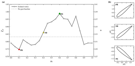
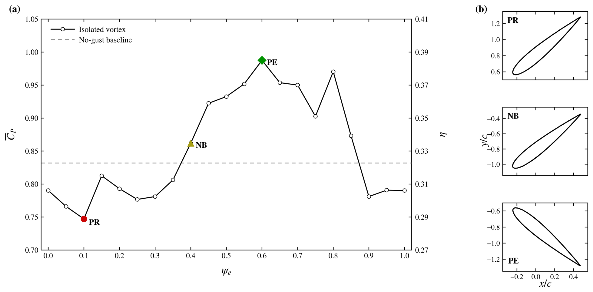
Figure 2a shows a pronounced phase dependence at fixed vortex parameters and body-fixed offset. The mean power coefficient ranges from to , compared with the no-gust value of . The sampled phases reduce the mean power below the no-gust level. Enhancement occurs over . Near the end of the cycle, the response falls below the baseline again. The prescribed kinematics and swept height remain unchanged, so follows the same relative variation as . The phase sweep demonstrates the sensitivity of the power response to the prescribed nominal encounter phase. The identified phase intervals apply to the present vortex and foil kinematics. They should not be interpreted as universal operating set points.
Figure 2.
(a) Mean power coefficient and hydrodynamic efficiency as functions of the fractional encounter phase . The horizontal dashed line denotes the no-gust baseline. (b) Foil attitudes at the nominal encounter instants for the representative power-reducing (PR), near-baseline (NB), and power-enhancing (PE) cases.
Three sampled phases are retained for the subsequent flow-field and parametric analyses. PR corresponds to the sampled minimum, at . NB is selected at , the first sampled phase above the no-gust value, with . PE corresponds to the sampled maximum, at . Figure 2b shows the corresponding foil attitudes at the nominal encounter times. PR and NB have the same pitching angle at the nominal encounter, °, but opposite heave positions: for PR and for NB.
To further quantify the influence of the encounter phase, the energy-harvesting performance of the no-gust baseline and the three representative cases is summarized in Table 1. The relative efficiency change is defined as
where denotes the no-gust efficiency.
Table 1.
Energy-harvesting performance of the no-gust baseline and the representative power-reducing (PR), near-baseline (NB), and power-enhancing (PE) encounter cases.
Relative to the no-gust baseline, the energy-harvesting efficiency decreases by for PR and increases by and for NB and PE, respectively. The labels PR, NB, and PE denote representative response classes. They are not intended to represent equally spaced performance levels.
4.1.2. Transient Aerodynamic and Power Responses
At zero body-fixed offset, the scheduled vortex-center target coincides with the pitching pivot at . The Taylor vortex induces velocity over a finite region. The foil loading may begin to depart from the no-gust response before the vortex center reaches the scheduled target. In the following comparisons, serves as a geometric phase reference and does not mark the onset of the transient response.
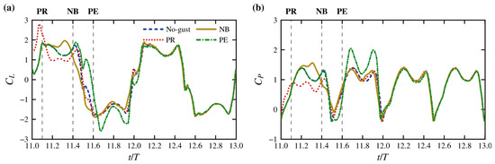
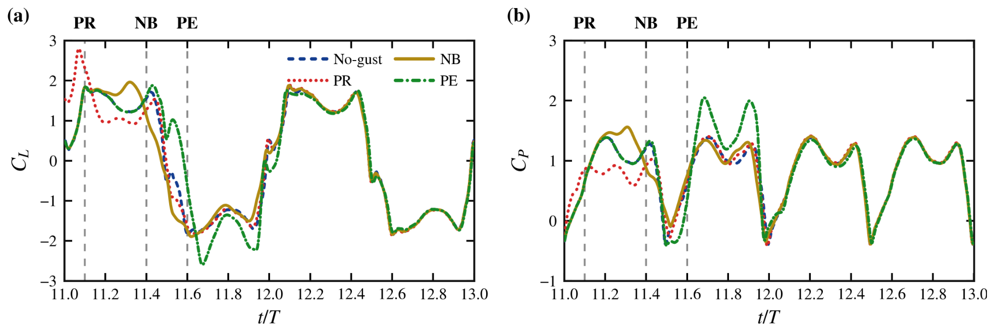
As shown in Figure 3, the isolated Taylor vortex causes transient deviations in both and from the periodic no-gust response. The magnitude and temporal evolution of these deviations depend on the nominal encounter phase. After the main interaction has subsided, the curves gradually approach the no-gust response, indicating that the effect of an isolated vortex is transient rather than persistent.
Figure 3.
Time histories of (a) the lift coefficient and (b) the instantaneous power coefficient for the representative PR, NB, and PE isolated-vortex encounters and their phase-matched no-gust references. The vertical dash-dotted lines mark the nominal encounter times.
For PR, the positive-power contribution is weakened during the early post-encounter stage. Over , the local maximum of decreases from for the phase-matched no-gust response to , while the interval-averaged value decreases from to . NB exhibits a smaller net departure from the baseline: its force and power histories remain between the PR and PE responses, consistent with the near-baseline nominal-encounter-aligned mean reported in Table 1.
PE produces the largest positive-power excursion. Its local maximum reaches at . The phase-matched no-gust maximum over the corresponding interval is . Under the chord-based normalization defined in Section 2.3, is a power coefficient, not a conversion efficiency. Values above unity are admissible.
The magnitude of the response also increases. It reaches at , compared with for the phase-matched no-gust case. The extremum and peak occur at nearly the same time. Their temporal proximity links both responses to the same gust-induced interaction. This correspondence does not isolate the transverse-force contribution to the extracted power. The total contains both heaving and pitching work. A force extremum alone cannot identify their separate contributions. The phase-resolved pressure and vorticity fields are examined next to show how the distributed loading changes during the PR and PE encounters.
4.1.3. Flow-Field Interpretation of the Encounter-Phase Effect
PR and PE bound the sampled power response and are selected for detailed flow-field analysis. Each isolated encounter is compared with a phase-matched no-gust solution. This comparison separates changes caused by the incoming vortex from the periodic flow generated by the prescribed foil motion. Phase matching is necessary because the foil has different attitudes at the respective nominal encounter times in the PR and PE cases. The selected snapshots follow the interaction from vortex approach through interaction to subsequent recovery. NB is not included because its cycle-averaged response remains close to the no-gust baseline.
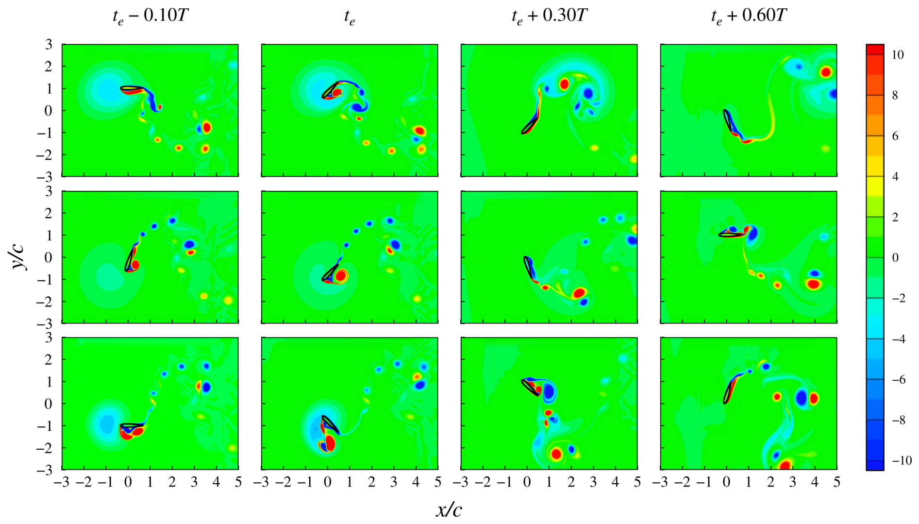
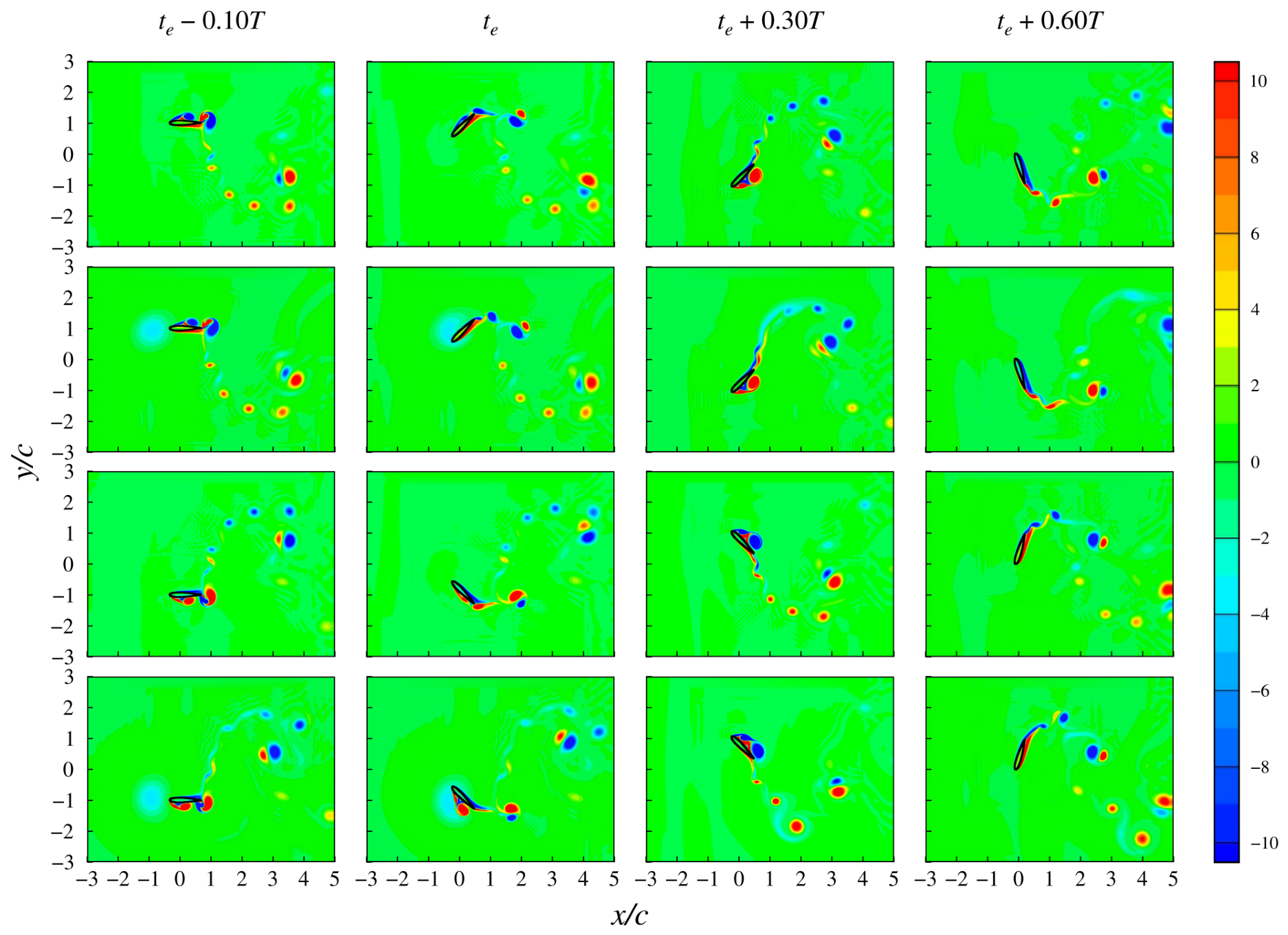
The corresponding phase-matched vorticity fields are shown in Figure 4. At , the incident Taylor vortex remains upstream of the foil. Even so, its induced velocity has already altered the near-foil flow relative to the phase-matched no-gust field. By , the vortex has deformed and begun to interact with vorticity generated along the foil surface. The subsequent sequence differs between PR and PE. In PR, the disturbed vorticity is stretched along the foil and carried into the downstream wake. The coupled structures remain close to the foil only briefly, and the near-foil disturbance weakens during the later snapshots.
Figure 4.
Instantaneous dimensionless spanwise-vorticity fields for the PR and PE isolated-vortex encounters and their phase-matched no-gust references. From top to bottom, the rows correspond to No-gust (PR), PR, No-gust (PE), and PE. From left to right, the columns correspond to , , , and . The common color scale represents .
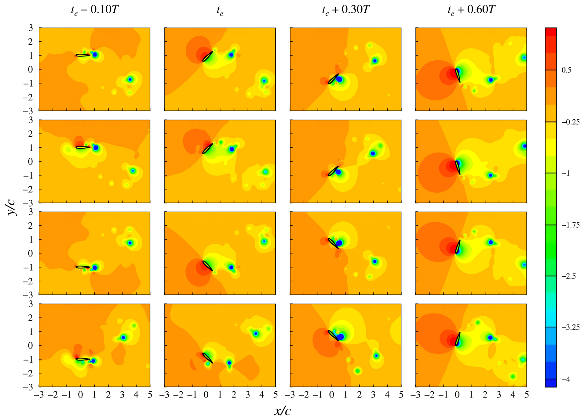
In PE, the incident vortex stays closer to the foil-generated vorticity after the nominal encounter. Their interaction leaves a more persistent reorganization of the near wake at and . The contrast between PR and PE involves both the near-foil residence and downstream development of the disturbance. These vorticity fields show how the structures evolve, but they do not determine whether the associated loading performs positive or negative work. The pressure fields in Figure 5 provide the corresponding loading information.
Figure 5.
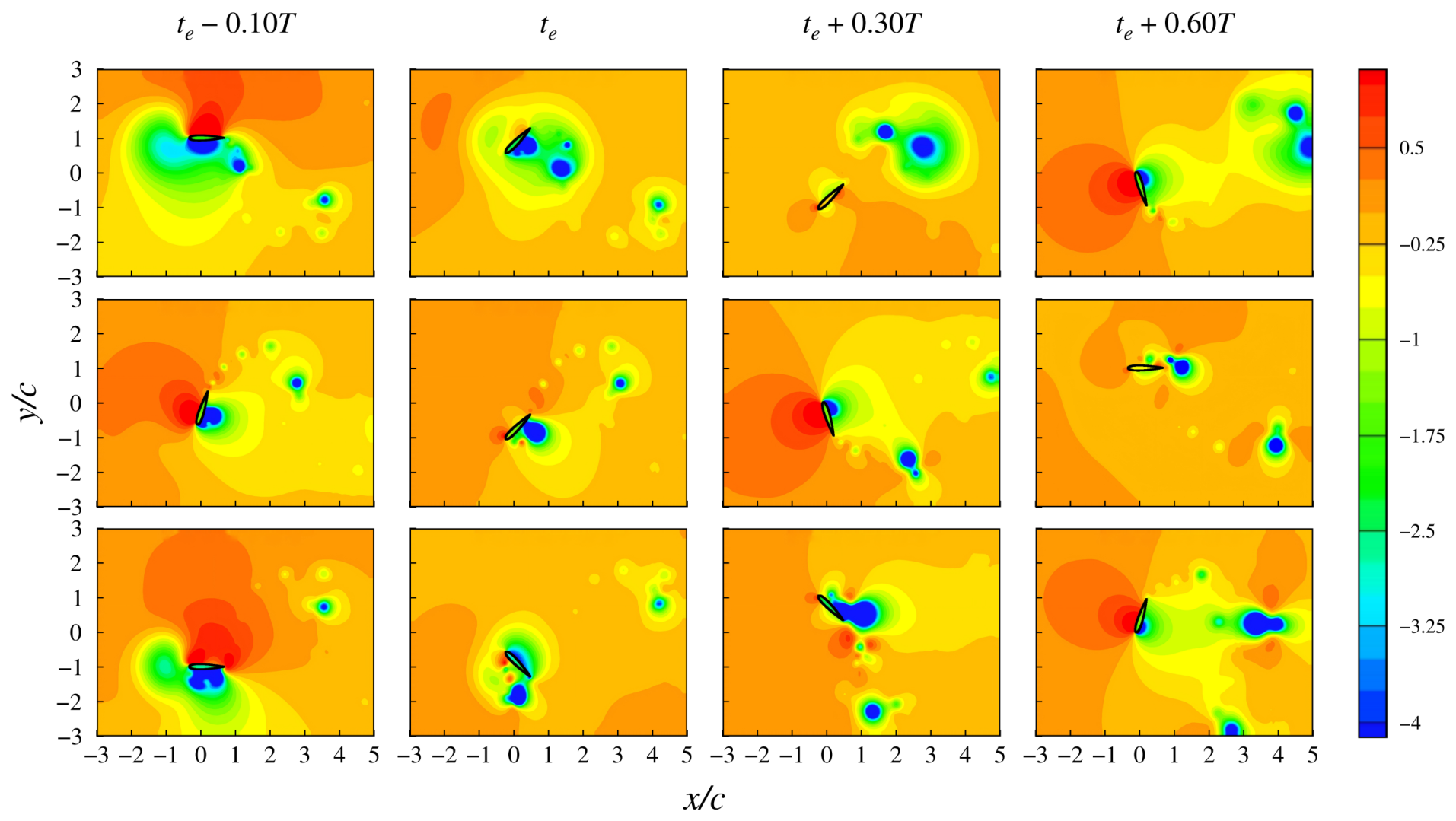
Instantaneous pressure-coefficient fields for the PR and PE isolated-vortex encounters and their phase-matched no-gust references. From top to bottom, the rows correspond to No-gust (PR), PR, No-gust (PE), and PE. From left to right, the columns correspond to , , , and . The common color scale represents .
At , the incoming vortex has already produced a localized pressure disturbance near the foil. The pressure distributions in both cases then depart further from their phase-matched no-gust fields. Their later responses differ markedly. In PR, the vortex redistributes the near-foil pressure field, but the resulting pattern is poorly aligned with the positive-work portion of the prescribed motion. The disturbance is subsequently convected downstream. This evolution is consistent with the weakened positive-power contribution in Figure 3b. In PE, a pronounced near-foil pressure contrast persists through the later interaction and recovery stages. Its persistence coincides with the larger positive excursion of in Figure 3b. The key difference is timing. The vortex-induced pressure loading acts more favorably relative to the prescribed foil motion in PE than it does in PR. The combined fields suggest that the longer near-foil residence changes when the pressure loading acts. Loading magnitude alone does not explain the difference between PR and PE.
4.2. Effects of Vortex Characteristics and Body-Fixed Offset
The following analysis examines the effects of vortex diameter, vortex intensity, and body-fixed offset at the representative PR, NB, and PE phases. Because the prescribed foil kinematics and swept height remain unchanged, is used as the primary performance metric; follows the same relative variation.
4.2.1. Effects of Vortex Diameter and Intensity
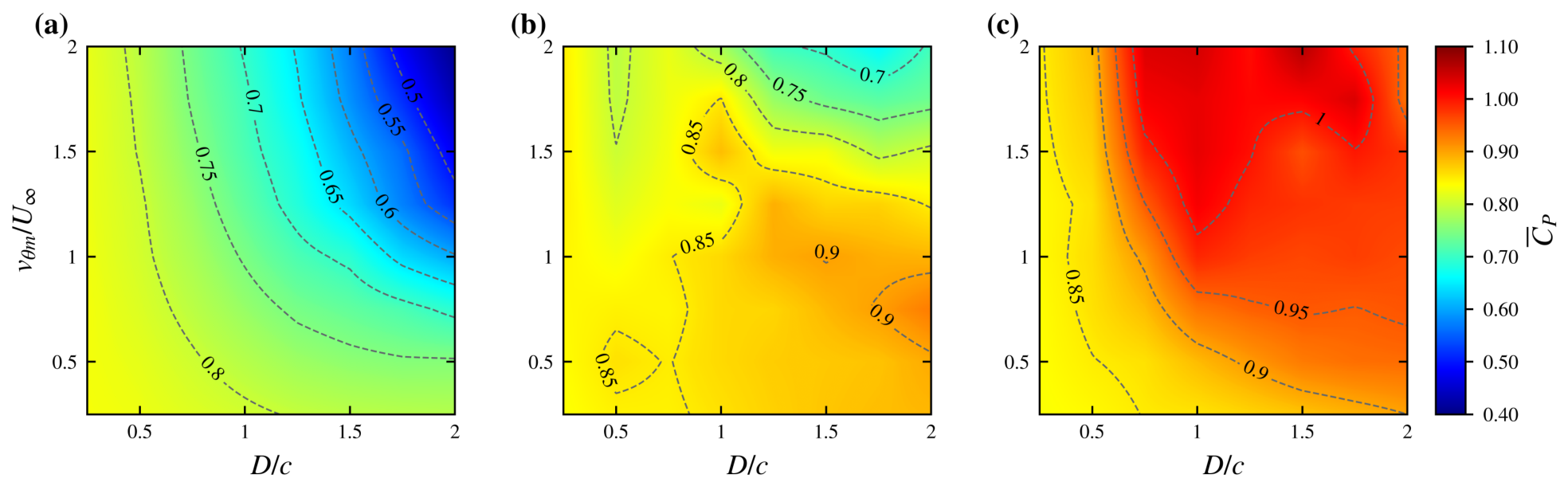
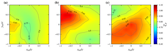
Vortex diameter and intensity are first varied for pivot-centered nominal encounters, with . At each representative PR, NB, and PE phase, and are sampled independently at , yielding 64 diameter–intensity combinations per phase. Figure 6 presents the resulting mean-power maps.
Figure 6.
Mean power coefficient in the – plane for pivot-centered encounters: (a) PR, (b) NB, and (c) PE.
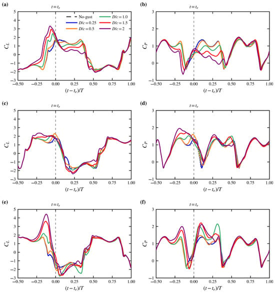
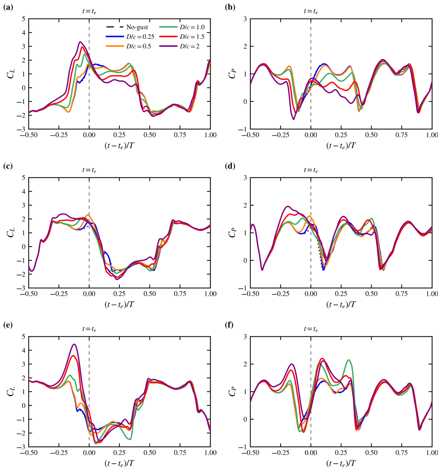
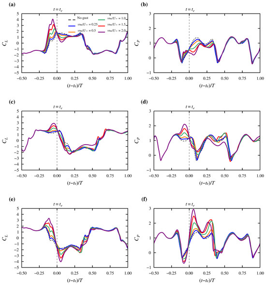
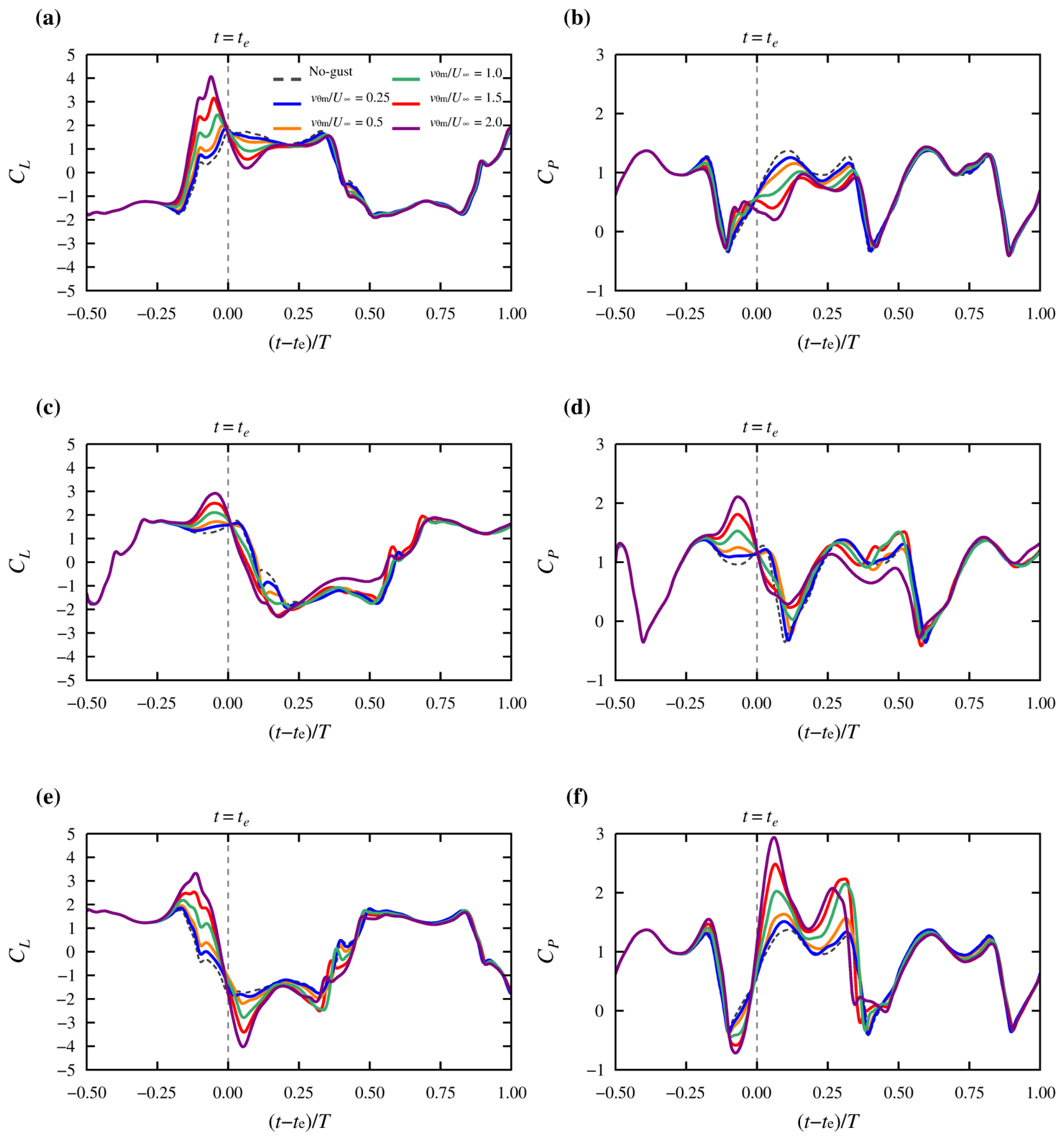
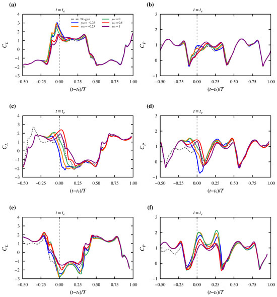
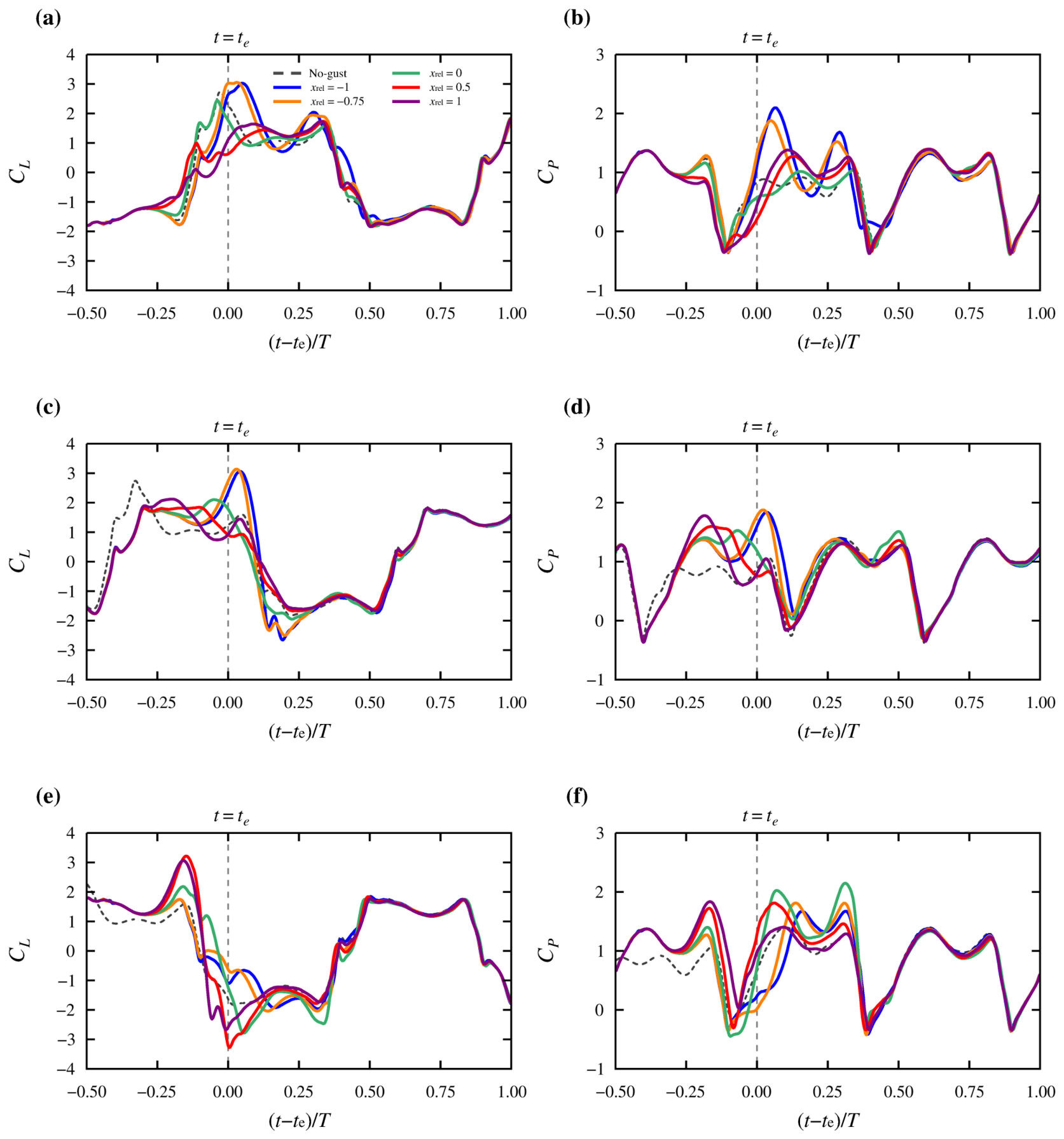
Two sections through each map are used to examine the transient response. One varies at fixed . The other varies at fixed . Figure 7 and Figure 8 show the corresponding lift and power histories. Time is measured relative to the nominal encounter, with at .
Figure 7.
Time histories of and for selected vortex diameters under pivot-centered encounters, with . Panels (a,b) show PR, (c,d) NB, and (e,f) PE. In each pair, is shown on the left and on the right. The vertical dashed line marks , and each panel includes a phase-matched no-gust reference.
Figure 8.
Time histories of the lift coefficient and instantaneous power coefficient for selected vortex intensities under pivot-centered encounters, with . Panels (a,b), (c,d), and (e,f) correspond to PR, NB, and PE, respectively; is shown in the left column and in the right column. The vertical dashed lines mark , and the no-gust response is included as a phase-matched reference.
Figure 6 reveals distinct phase-dependent response regions in the – space. In the PR phase, the low-power region expands toward larger and larger , with decreasing from at to at . In the NB phase, the high-power region is confined to moderate-to-large diameters and intermediate intensities, reaching at , whereas stronger vortices reduce the harvested power. By contrast, the PE phase exhibits a broader high-power region, with the largest sampled value, , occurring at . Thus, the energetic effect of increasing vortex size or intensity depends on the encounter phase and may be suppressive, near-baseline, or enhancing.
Figure 7 shows that the vortex diameter mainly changes the duration and persistence of the vortex-induced loading. In the PR phase, increasing broadens the interval over which both and depart from the no-gust response. This extended disturbance is not synchronized with the useful power-producing portion of the cycle and therefore reduces the mean harvested power from to . In the NB phase, intermediate and large diameters extend the favorable portion of the response, but the resulting gain is non-monotonic, indicating that an excessively broad disturbance does not necessarily improve power extraction. In the PE phase, increasing strengthens the positive-power response up to , beyond which the time histories change only weakly and the mean harvested power becomes less sensitive to further increases in diameter.
Figure 8 indicates that the vortex intensity primarily changes the magnitude of the induced unsteady loading, but its energetic consequence remains strongly phase-dependent. In the PR phase, stronger vortices increase the departure of both and from the no-gust response. Because this intensified loading occurs over an unfavorable portion of the cycle, decreases from at to at . This trend is consistent with the expansion of the low-power region in Figure 6a. In the NB phase, the response is non-monotonic: moderate-to-high intensities enlarge the useful-power portion of the cycle, with reaching at , whereas a further increase to weakens the favorable power response and reduces to . By contrast, the PE phase converts stronger vortex-induced loading into a more favorable power response, increasing from to over the same intensity range.
Across the selected one-parameter sections, diameter is associated mainly with disturbance duration and persistence, whereas intensity is associated mainly with loading magnitude; these tendencies remain coupled. Diameter changes how long the disturbance remains influential. Intensity changes the scale of the induced loading. The field comparisons below connect these trends to the near-foil vorticity and pressure distributions.
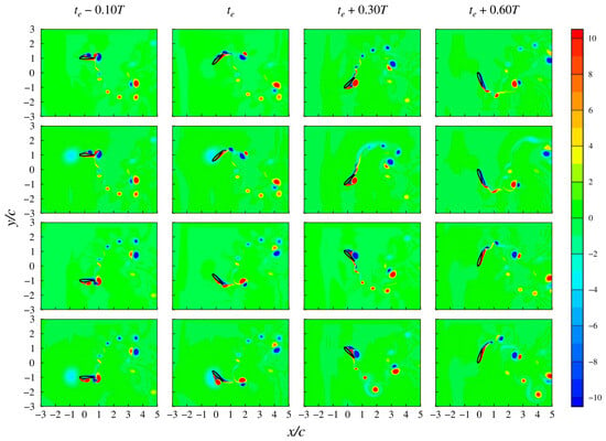
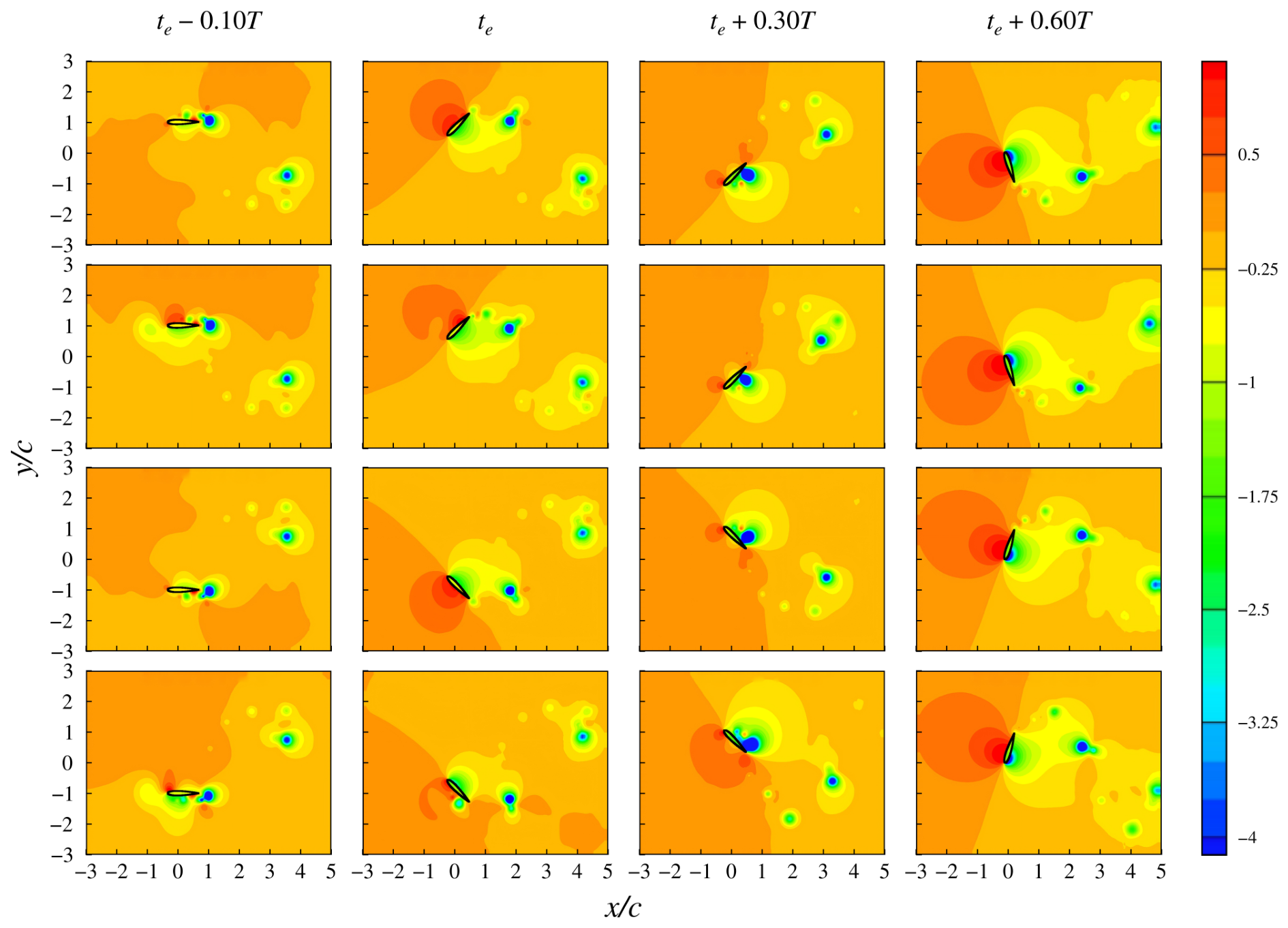
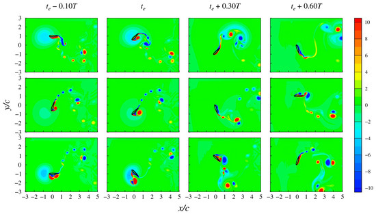
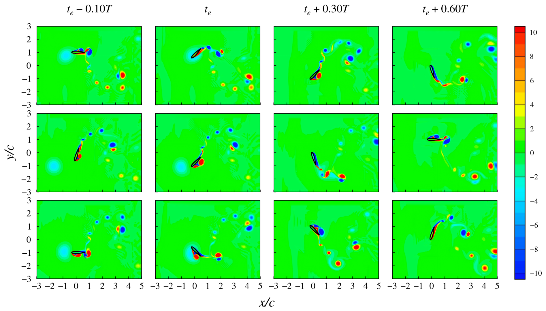
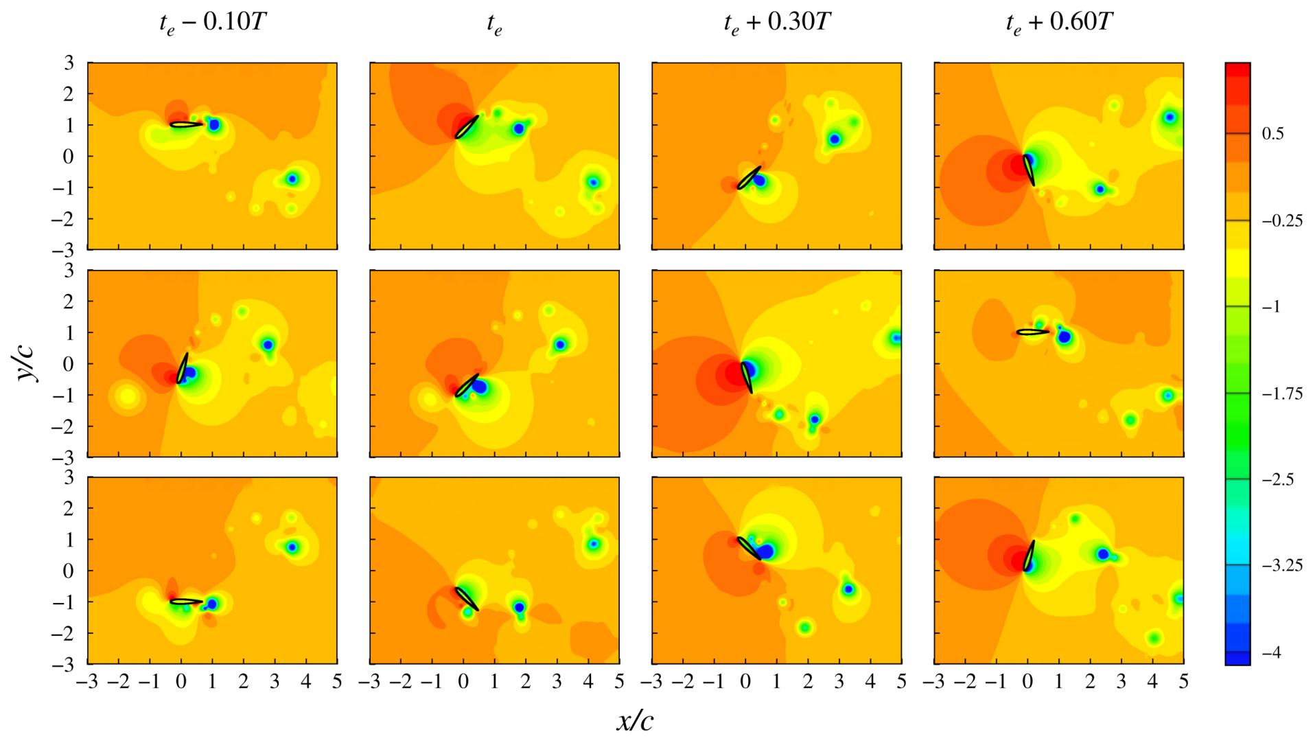
Three cases are selected from distinct regions of Figure 6. The PR case uses , the NB case uses , and the PE case uses . Figure 9 and Figure 10 follow these interactions from vortex approach to recovery.
Figure 9.
Instantaneous dimensionless spanwise-vorticity fields for the PR, NB, and PE cases selected from the response maps. From top to bottom, the rows show PR, NB, and PE. From left to right, the columns correspond to , 0, , and .
Figure 10.
Instantaneous pressure-coefficient fields for the PR, NB, and PE cases selected from the response maps. From top to bottom, the rows show PR, NB, and PE. From left to right, the columns correspond to , 0, , and .
Figure 9 and Figure 10 further show how the diameter–intensity response is linked to the organization of the incoming vortex, the foil-generated vortical structures, and the associated pressure loading. In the PR case, the large and strong vortex occupies a broad region around the foil and substantially distorts the near wake after the nominal encounter. The pressure field also develops an extended low-pressure region that is not well aligned with the useful power-producing portion of the foil motion, consistent with the low-power region in Figure 6.
The NB case shows a less disruptive interaction. The vortex remains large enough to modify the near-foil pressure distribution, but its moderate intensity avoids the strong subsequent wake distortion observed in the PR case. As a result, the pressure difference is strengthened during part of the cycle without producing persistent adverse loading, which is consistent with the local high-power region at intermediate intensity in Figure 6.
For the PE case, the incoming vortex interacts more favorably with the foil-generated vortical structures. During the interaction-development stage, the pressure field maintains a stronger low-pressure region on the power-producing side of the foil, in agreement with the enhanced positive-power response in Figure 8. These snapshots therefore suggest that the diameter–intensity response is associated not only with the size and strength of the incoming vortex, but also with the temporal alignment between the induced pressure loading and the prescribed heaving–pitching motion.
4.2.2. Effects of Body-Fixed Encounter Offsets
The body-fixed encounter geometry is sampled by varying and independently from to in increments of . This produces 81 offset combinations at each representative phase. The prescribed vortex parameters remain fixed at and .
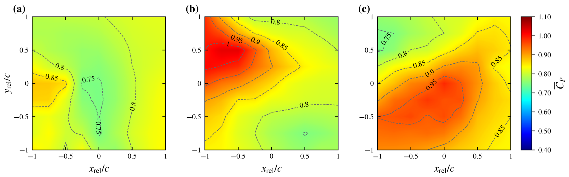
Figure 11 shows that the relative encounter offsets also produce strongly phase-dependent response regions in the – plane. In the PR phase, the low-power region is concentrated near the pivot-centered encounter location, with at and a minimum value of near . Moving the nominal vortex position toward negative chordwise offsets weakens this adverse effect, and increases to at . In the NB phase, the response becomes more strongly asymmetric: the high-power region is displaced toward negative and positive , reaching at , whereas a low-power region appears for positive chordwise offsets combined with negative normal offsets, with at . By contrast, the PE phase retains its most favorable response near the pivot-centered encounter, with a maximum value of at , while large upstream–upper offsets reduce the harvested power, giving at . These results indicate that the relative encounter location does not act as a simple geometric correction; rather, it determines whether the incoming vortex is spatially and temporally aligned with the foil-generated vortical structures and the power-producing pressure loading.
Figure 11.
Phase-dependent response maps of in the – plane. Panels (a–c) denote the PR, NB, and PE phases, respectively.
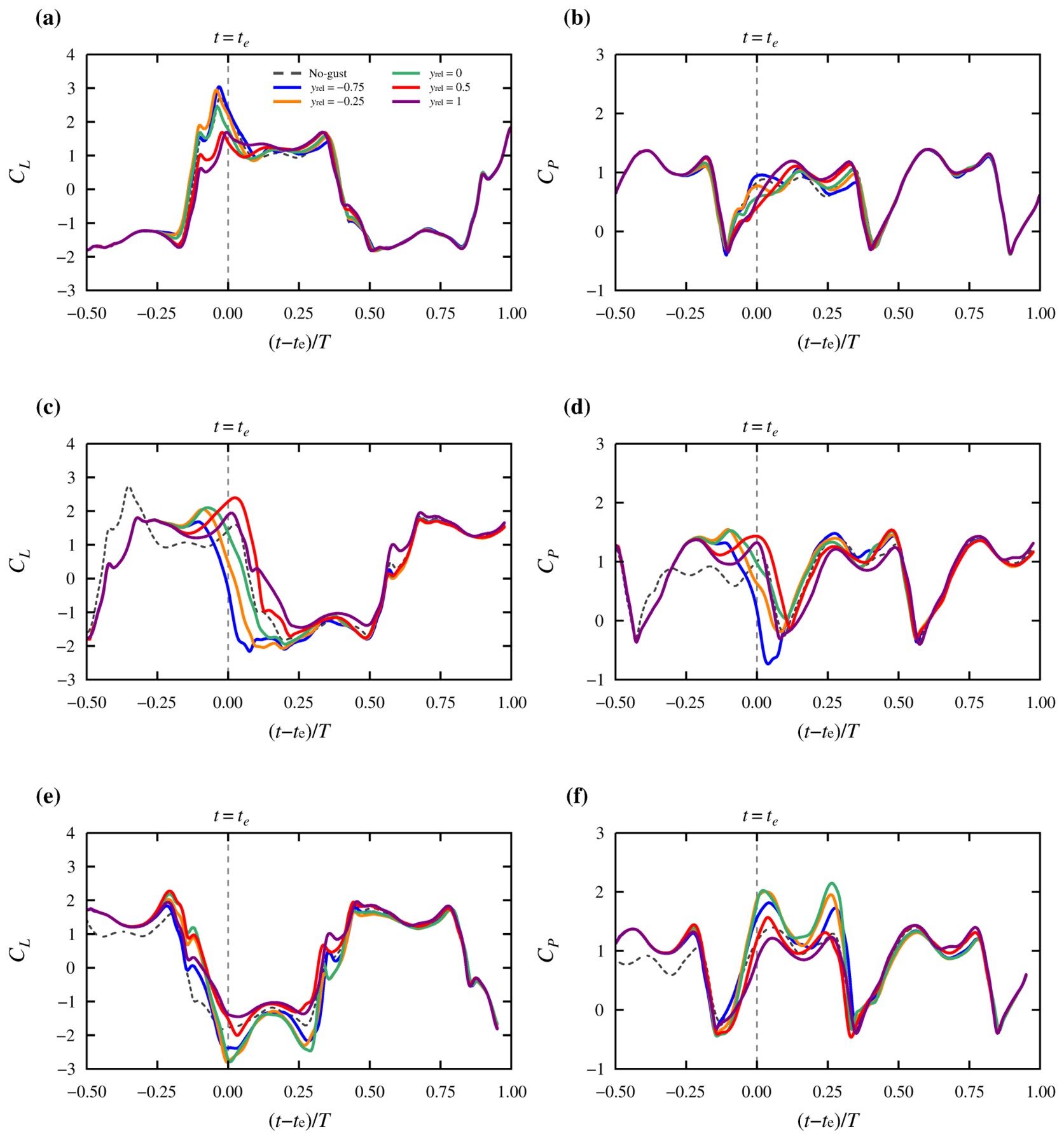
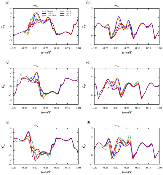
To relate the offset-dependent response regions to the transient aerodynamic loading, two representative sections of the – response maps are examined. The first section fixes and varies , , 0, , and to isolate the effect of normal offset, as shown in Figure 12. The second section fixes and varies , , 0, , and to examine the effect of chordwise offset, as shown in Figure 13. These two sections pass through the lower-/negative-offset, pivot-centered, and positive-offset regions identified in Figure 11. In both comparisons, the no-gust case is included as a reference, and the time axis is shifted relative to the nominal encounter instant, such that at .
Figure 12.
Time histories of and for selected normal encounter offsets at , with and . Panels (a,b), (c,d), and (e,f) correspond to the PR, NB, and PE encounter phases, respectively, with shown in the left column and in the right. The vertical dashed line marks the nominal encounter instant, , and the no-gust response is included as a reference.
Figure 13.
Time histories of and for selected chordwise encounter offsets at , with and . Panels (a,b), (c,d), and (e,f) correspond to the PR, NB, and PE encounter phases, respectively, with shown in the left column and in the right. The vertical dashed line marks the nominal encounter instant, , and the no-gust response is included as a reference.
Figure 12 shows that the normal offset modifies both the magnitude and timing of the vortex-induced force and power responses. In the PR phase, the centered and lower-side encounters generate a stronger departure from the no-gust response during the interaction stage, but this departure does not coincide with a sustained positive-power excursion. As a result, the instantaneous response is weakened over part of the cycle, leading to low mean power values of at and at . When the vortex is shifted toward the positive normal side, the adverse portion of the power response is reduced, and increases to at . In the NB phase, the histories indicate a non-monotonic offset effect: increasing from to prolongs portions of the positive-power response and raises from to , whereas a further increase to weakens the interaction and reduces to . In the PE phase, the pivot-centered encounter produces the strongest positive-power response along this section, with at . Positive normal offsets weaken the transient power response, indicating that the beneficial PE interaction requires the vortex-induced loading to remain close to the centered encounter path. These results suggest that the normal offset mainly controls the side on which the induced loading acts and whether this loading develops during positive- or negative-work portions of the prescribed motion.
Figure 13 further shows that the chordwise offset primarily changes the timing of the vortex–foil interaction. In the PR phase, the pivot-centered encounter produces a low-power response, with at . Shifting the vortex toward negative chordwise offsets changes the timing of the induced loading relative to the foil motion and reduces the unfavorable power response, increasing to and at and , respectively. In the NB phase, the histories also show that negative chordwise offsets are more favorable, with at and at , whereas positive offsets shorten or weaken the useful-power interval and reduce the mean harvested power. The PE phase responds differently: its strongest transient power response occurs near the pivot-centered encounter, where at , and moving the vortex either upstream or downstream weakens the positive-power response. Therefore, the chordwise offset does not simply shift the vortex to a more or less favorable geometric position; rather, chordwise offset primarily shifts the timing at which the incoming vortex interacts with the foil-generated structures.
The two sections reveal different roles for the body-fixed offsets. Normal displacement changes the side of the foil affected by the vortex and the degree of spatial overlap. Chordwise displacement mainly changes when the interaction occurs. The effects remain coupled. Mean power depends on how the resulting force and moment histories align with the positive- and negative-work portions of the prescribed motion. Phase and offset must be considered together.
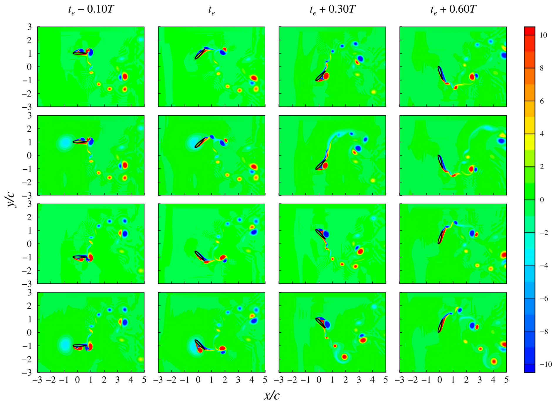
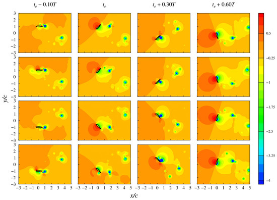
Three offset combinations are selected from Figure 11. PR uses , NB uses , and PE uses . All three cases retain and . Figure 14 and Figure 15 follow the interactions from vortex approach to recovery.
Figure 14.
Instantaneous dimensionless spanwise-vorticity fields for the PR, NB, and PE cases selected from the response maps. From top to bottom, the rows show PR, NB, and PE. From left to right, the columns correspond to , 0, , and .
Figure 15.
Instantaneous pressure-coefficient fields for the PR, NB, and PE cases selected from the response maps. From top to bottom, the rows show PR, NB, and PE. From left to right, the columns correspond to , 0, , and .
Figure 14 and Figure 15 further illustrate how the encounter offsets reorganize the vortex–foil interaction and the associated pressure loading. In the PR case, where the vortex is placed slightly below the pivot-centered path, the induced vortical structures remain close to the foil during the nominal-encounter and interaction-development stages. However, the resulting pressure field is not favorably phased with the power-producing portion of the motion. The localized low-pressure region near the foil does not develop into a sustained favorable pressure difference, consistent with the low-power response of the centered and lower-side encounters in Figure 12.
The NB case shows a more favorable offset-induced organization. With a negative chordwise and positive normal offset, the incoming vortex interacts with the foil-generated vortical structures without producing strong adverse near-wake distortion. Meanwhile, the pressure field develops a more coherent low-pressure region on the power-producing side of the foil during the interaction-development stage. This behavior is consistent with the enlarged useful-power interval in Figure 13 and with the high-power region near and in Figure 11.
For the PE case, the pivot-centered encounter remains the most favorable configuration among the selected offset sections. The incoming vortex interacts with the foil-generated vortical structures close to the nominal encounter path, and the pressure field maintains a stronger favorable pressure difference during the interaction stage. Thus, unlike the NB case, the beneficial PE response does not require an upstream or normal displacement of the vortex; it results from favorable alignment between the vortex-induced loading and the prescribed heaving–pitching motion.
For vortical inflows with a repeatable or predictable dominant path, the phase and offset maps provide conditional guidance for coordinating foil motion and placement. For the same pivot-centered nominal encounter target, , power was enhanced at but reduced at , indicating that the energetic response depends on the prescribed nominal encounter phase.
The numerical phase and offset values apply only to the present Taylor vortex and prescribed kinematics. Other inflow or device conditions require recalibration.
The offset trends are qualitatively consistent with previous fixed-airfoil vortical-gust studies. At , Martínez-Muriel and Flores [17] reported that the time to peak lift scales with and that the peak magnitude is approximately proportional to vortex circulation. They also found a nonlinear dependence on vertical separation. More recent high-fidelity studies identify similar sensitivity to vortex strength, size, initial position, and airfoil geometry [21,22].
The present moving-foil results retain these loading sensitivities but add an energetic constraint. A load change can increase or decrease harvested power according to its timing relative to the prescribed foil velocity. Differences in geometry, kinematics, Reynolds number, and gust definition prevent a one-to-one quantitative comparison. The agreement supports qualitative physical consistency.
4.3. Effects of Sustained Periodic-Vortical Encounters
The isolated-vortex results do not account for residual disturbances left by earlier encounters. To determine whether the phase-dependent ordering survives when those disturbances accumulate, the reference Taylor vortex ( and ) is introduced at the pivot-centered target once per flapping period. Ten same-sign vortices are applied in each PR, NB, and PE sequence, with successive nominal encounter times separated by T and the corresponding fractional phase held fixed.
For encounter index k, the cycle-resolved mean power coefficient is
where denotes the nominal time of the kth encounter. The initial encounters describe the transition from the phase-matched no-gust state to the repeated-encounter response. The sustained mean is evaluated over the five nearly repeatable encounters –9:
The corresponding hydrodynamic efficiency is , using the same swept height as in the isolated-vortex cases.
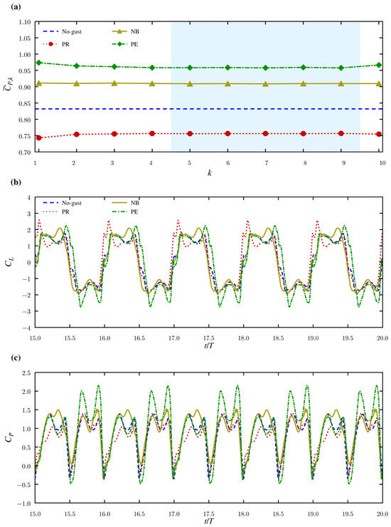
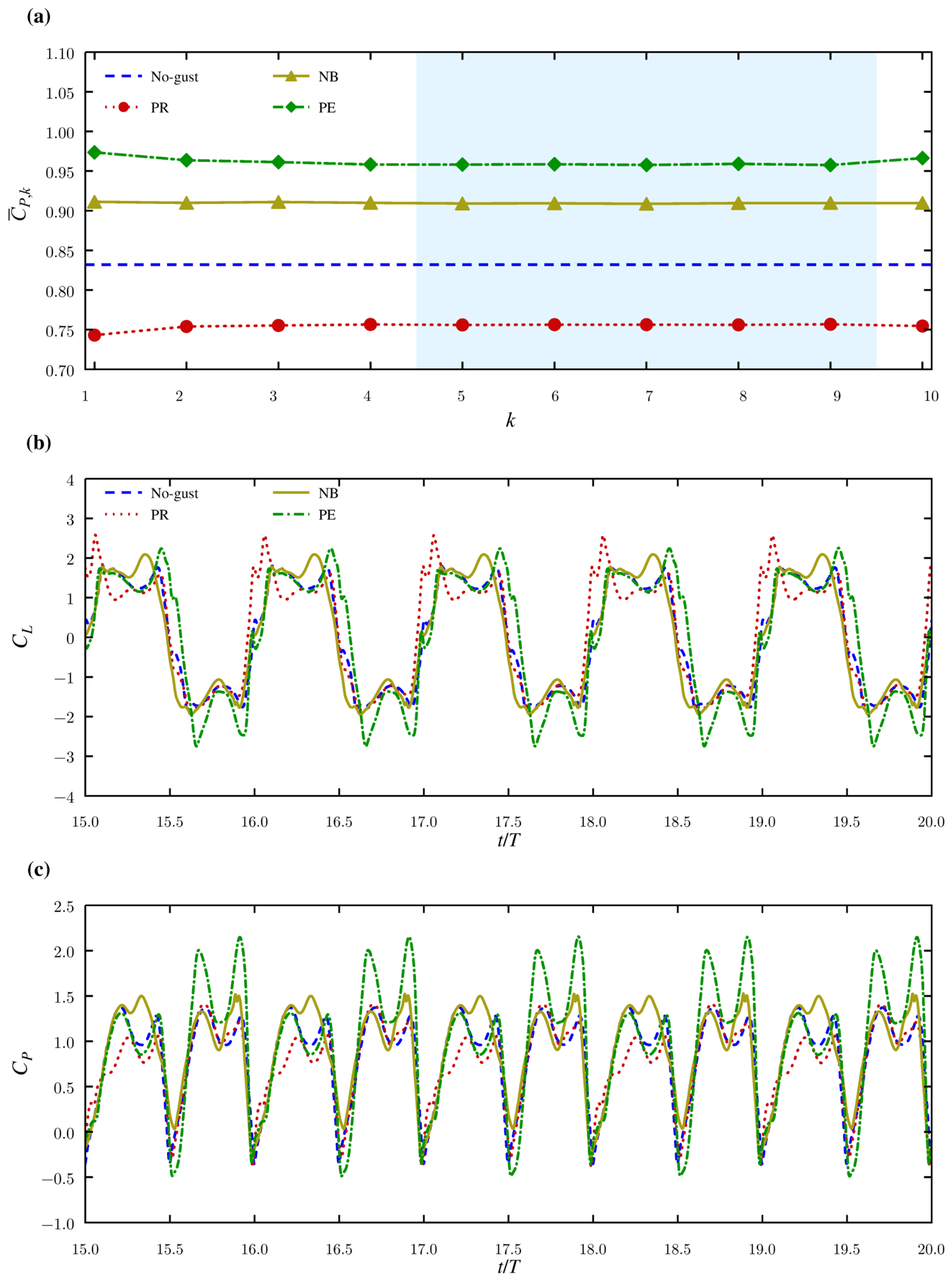
Figure 16a shows an initial adjustment over the first few encounters as the imposed vortex train modifies the pre-existing foil wake. By , the cycle means are nearly repeatable. PR remains below the no-gust baseline throughout –9. NB and PE remain above it. The sign of the isolated-encounter response is therefore preserved under repeated forcing, even though the incoming wake has changed.
Figure 16.
Responses to repeated vortical encounters. (a) Cycle-resolved mean power coefficient . The shaded region identifies encounters –9, which are used to evaluate . (b) Lift coefficient and (c) instantaneous power coefficient over , the nearly repeatable interval spanning encounters –9.
Figure 16b,c cover the same sustained interval, . The waveforms repeat closely from one cycle to the next. PR loses positive power over a substantial part of each cycle. NB and PE show larger positive-power excursions than their phase-matched no-gust references, and PE retains the largest peaks and highest sustained mean. The same ordering appears in both the instantaneous histories and the cycle-resolved means. It is not created by averaging a single transient.
Table 2 summarizes the no-gust, isolated-encounter, and repeated-encounter performance. PR remains the lowest-response case. The no-gust value lies between PR and NB, and PE remains highest.
Table 2.
Comparison of mean power coefficients and hydrodynamic efficiencies for the no-gust, isolated-encounter, and repeated-encounter cases. For the no-gust and isolated-encounter cases, the reported quantities are and ; for the repeated-encounter cases, they are and .
Repeated forcing does not shift the three phases in the same direction. For PR, the mean increases by (), and the efficiency penalty relative to the no-gust baseline narrows from to .
NB shows the largest gain. Its mean rises by (), and the efficiency enhancement increases from to .
PE changes in the opposite direction. Its mean decreases by (), while the efficiency enhancement falls from to . The wake retained from earlier encounters alters each phase differently. A sustained response cannot be estimated by simply repeating the isolated nominal-encounter-aligned mean.
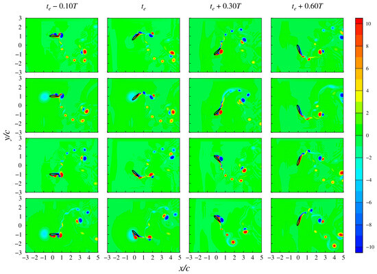
To examine the flow-field changes associated with repeated encounters, PR and PE are compared with phase-matched no-gust references at the same normalized times and foil attitudes. These cases bound the repeated-encounter performance range, while NB remains represented in Figure 16 and Table 2. The corresponding vorticity and pressure-coefficient fields are shown in Figure 17 and Figure 18, respectively.
Figure 17.
Instantaneous dimensionless spanwise vorticity fields for the representative PR and PE cases under sustained periodic-vortical encounters and their phase-matched no-gust references. From top to bottom, the rows correspond to No-gust (PR), PR, No-gust (PE), and PE, respectively, while the columns show successive stages of the vortex–foil encounter.
Figure 18.
Instantaneous pressure-coefficient fields for the representative PR and PE cases under sustained periodic-vortical encounters and their phase-matched no-gust references. From top to bottom, the rows correspond to No-gust (PR), PR, No-gust (PE), and PE, respectively, while the columns show successive stages of the vortex–foil encounter.
Figure 17 and Figure 18 show how the vortex train modifies the near wake and pressure loading. In PR, each incoming vortex meets shear layers and remnants left by earlier cycles. Their roll-up and downstream convection differ from the phase-matched no-gust sequence. The near-foil low-pressure region is also displaced. This pressure change occurs during the reduced positive-power interval in Figure 16c, consistent with an adverse load–velocity alignment.
PE follows a different sequence, although the imposed vortices and repetition period are unchanged. Interaction with the residual wake maintains a favorable near-foil pressure difference during the positive-power portion of the motion. The result is a stronger excursion and a positive sustained mean. The periodic response depends on where and when each new vortex meets both the foil and the wake retained from earlier cycles.
The repeated sequences retain a phase relation between each newly imposed vortex and the wake left by earlier cycles. Variations in the timing of the prescribed foil motion relative to this combined disturbance are consistent with differences in whether the associated loading performs positive or negative work.
This interpretation is qualitatively consistent with tandem-foil measurements showing that downstream efficiency varies with inter-foil phase [23]. A later wake–foil model related the time-dependent power to the incident wake and foil kinematics [24]. Handy-Cardenas et al. [25] identified favorable regimes that either avoid coherent vortices or interact with them directly. Ren et al. [26] similarly distinguished constructive and destructive vortex–foil interaction modes according to the encounter geometry and vortex rotation.
Periodic vortical forcing is also experimentally feasible. Rockwood and Medina [27] generated repeatable gusts with controlled frequency, strength, and transverse position. Their experiment supports synchronized encounters of the type idealized here, although the present insertion method does not reproduce a specific physical gust generator.
A one-to-one quantitative comparison is not appropriate. The cited studies differ in foil geometry and motion, Reynolds number, vortex-generation method, and performance normalization. The comparison is limited to qualitative phase dependence, flow-field interpretation, and the feasibility of synchronized forcing.
4.4. Application Implications and Model Scope
The response maps provide conditional hydrodynamic guidance for wake-dominated inflows with a repeatable or sufficiently predictable vortex path and prescribed nominal encounter phase. Under such conditions, foil placement and motion timing may be coordinated to increase the likelihood that vortex-induced loading acts during positive-work portions of the cycle. The repeated encounters illustrate the importance of this coordination. Relative to the no-gust baseline, PE increases the hydrodynamic efficiency by , whereas PR reduces it by under the same vortex parameters and repetition period. The energetic effect of a coherent vortex therefore depends on when and where it encounters the foil.
For irregular inflows, encounter phase, vortex path, scale, and strength should be treated statistically rather than as fixed operating values. Any active use of the response maps would also depend on sensing and prediction accuracy, actuator bandwidth, and structural and power-take-off constraints.
The quantitative results apply to a two-dimensional laminar calculation at for one foil geometry and one prescribed heaving–pitching motion. The Taylor vortex is introduced independently of a physical generating body, and the repeated cases use one same-sign vortex per period. This controlled formulation permits phase-conditioned comparisons of loading and power but does not represent three-dimensional vortex deformation, transition, broadband turbulence, or generator-specific variability. The reported phase ranges should therefore not be transferred directly to other vortex profiles or operating conditions.
The reported power is the hydrodynamic work transferred to the prescribed foil motion. Structural feedback, power-take-off dynamics, mechanical transmission, control expenditure, and electrical conversion losses are not included. The present trends therefore do not guarantee net device performance. Their extension requires experimentally generated vortex trains, three-dimensional and higher-Reynolds-number simulations, and coupled fluid–structure–power-take-off models.
5. Conclusions
This study prescribed the Taylor vortex independently of any upstream generating body while keeping the foil kinematics fixed. The resulting framework allowed the effects of encounter phase, body-fixed offset, vortex diameter, and vortex intensity on hydrodynamic power extraction to be evaluated separately. For the zero-offset reference vortex (), the nominal-encounter-aligned mean power coefficient ranged from at to at , compared with the no-gust value of . Mean power was reduced over the sampled interval and enhanced over . The presence of a coherent vortex alone did not set the energetic response. For the reference vortex, prescribed nominal encounter phase was the primary discriminator between power suppression and enhancement.
Vortex diameter mainly changed the spatial extent and duration of the disturbance. Intensity acted primarily on the loading amplitude. Body-fixed offsets introduced two further effects: normal displacement altered the side of the foil affected and the degree of spatial overlap, while chordwise displacement shifted the interaction timing. The energetic effect of each variable changed with encounter phase. The field and power histories support a common physical interpretation. Across the sampled cases, enhancement was associated with favorable alignment between the vortex-induced pressure loading and a positive-work portion of the prescribed heaving–pitching motion.
The representative response ordering persisted under same-sign, once-per-cycle encounters. The sustained mean power coefficients were , , and for PR, NB, and PE, respectively. Relative to the corresponding isolated encounters, the PR and NB means increased by and , whereas the PE mean decreased by . These nonuniform shifts are consistent with wake memory. Residual structures from earlier cycles modified the loading produced by each new vortex, but did not reverse the phase ordering in the present cases. Repeated encounters cannot be represented as independent copies of an isolated event.
For vortical inflows with a repeatable or sufficiently predictable dominant path, encounter phase and foil placement should be considered jointly. The same pivot-centered nominal encounter target was power-enhancing at but power-reducing at ; thus, a centered target is not inherently favorable.
These conclusions apply to a two-dimensional laminar flow at , a single prescribed heaving–pitching motion, and an idealized Taylor vortex. The reported efficiency measures hydrodynamic energy transfer to the prescribed motion, not net device output. Three-dimensional effects, structural feedback, power-take-off dynamics, and conversion losses are outside the present model. The results provide conditional performance and flow-field guidance for controlled vortical encounters. They should not be interpreted as direct predictions of full-system performance.
Supplementary Materials
The following supporting information can be downloaded at: https://www.mdpi.com/article/10.3390/en19163931/s1.
Author Contributions
Project administration, funding acquisition, conceptualization, methodology, investigation, validation, formal analysis, resources and writing—original draft preparation, S.W. (Shihui Wu), X.W., H.Q., Z.Z., S.W. (Shaofeng Wu) and S.L.; supervision and writing—review and editing, L.W. All authors have read and agreed to the published version of the manuscript.
Funding
This research was funded by the Science and Technology Research Program of Chongqing Municipal Education Commission (Grant Nos. KJZD-K202401801, KJZD-K202501801, KJQN202401801, and KJZD-K202201801), the Natural Science Key Project of Chongqing College of Humanities, Science & Technology (Grant Nos. CRKZK202500 and CRKZKYB2026002), and the Scientific Research Project of Hechuan District Science and Technology Bureau (Grant Nos. HCKJ-2025-083 and HCKJ-2024-111).
Data Availability Statement
The minimal dataset supporting the figures and tables reported in this study is provided in the Supplementary Materials. Additional raw numerical outputs are available from the corresponding author upon reasonable request.
Acknowledgments
The authors would like to thank the anonymous reviewers for their constructive comments.
Conflicts of Interest
The authors declare no conflicts of interest.
Abbreviations
The following abbreviations are used in this manuscript:
| D2Q9 | Two-dimensional nine-velocity lattice model |
| GCI | Grid convergence index |
| IB–LBM | Immersed boundary–lattice Boltzmann method |
| LBM | Lattice Boltzmann method |
| MPI | Message Passing Interface |
| MRT | Multiple-relaxation-time |
| MRT–LBM | Multiple-relaxation-time lattice Boltzmann method |
| NB | Near-baseline response |
| OpenMP | Open Multi-Processing |
| PE | Power-enhancing response |
| pIB | Penalty immersed-boundary method |
| PR | Power-reducing response |
Appendix A. Computational Setup and Numerical Verification
The computational domain is and . A six-level nested multi-block grid covers the computational domain. Starting from an outermost spacing of , factor-of-two refinement gives the production spacing . The time step is refined by the same factor between adjacent levels, with in lattice units. The foil is discretized with Lagrangian spacing , and the refined region follows the prescribed motion. On the outermost block, the boundary treatment combines a non-reflecting condition with sponge relaxation toward the freestream state. The production calculations use and in lattice units. These values give . The production runs were performed using one Message Passing Interface(MPI) rank and eight Open Multi-Processing (OpenMP) threads.
Figure A1 illustrates the computational domain, the six-level nested multi-block grid, and the local grid arrangement around the foil. The minimum Eulerian grid spacing is , while the Lagrangian-marker spacing is .
Figure A1.
Computational domain and grid arrangement: (a) six-level nested multi-block grid; (b) local grid around the foil.
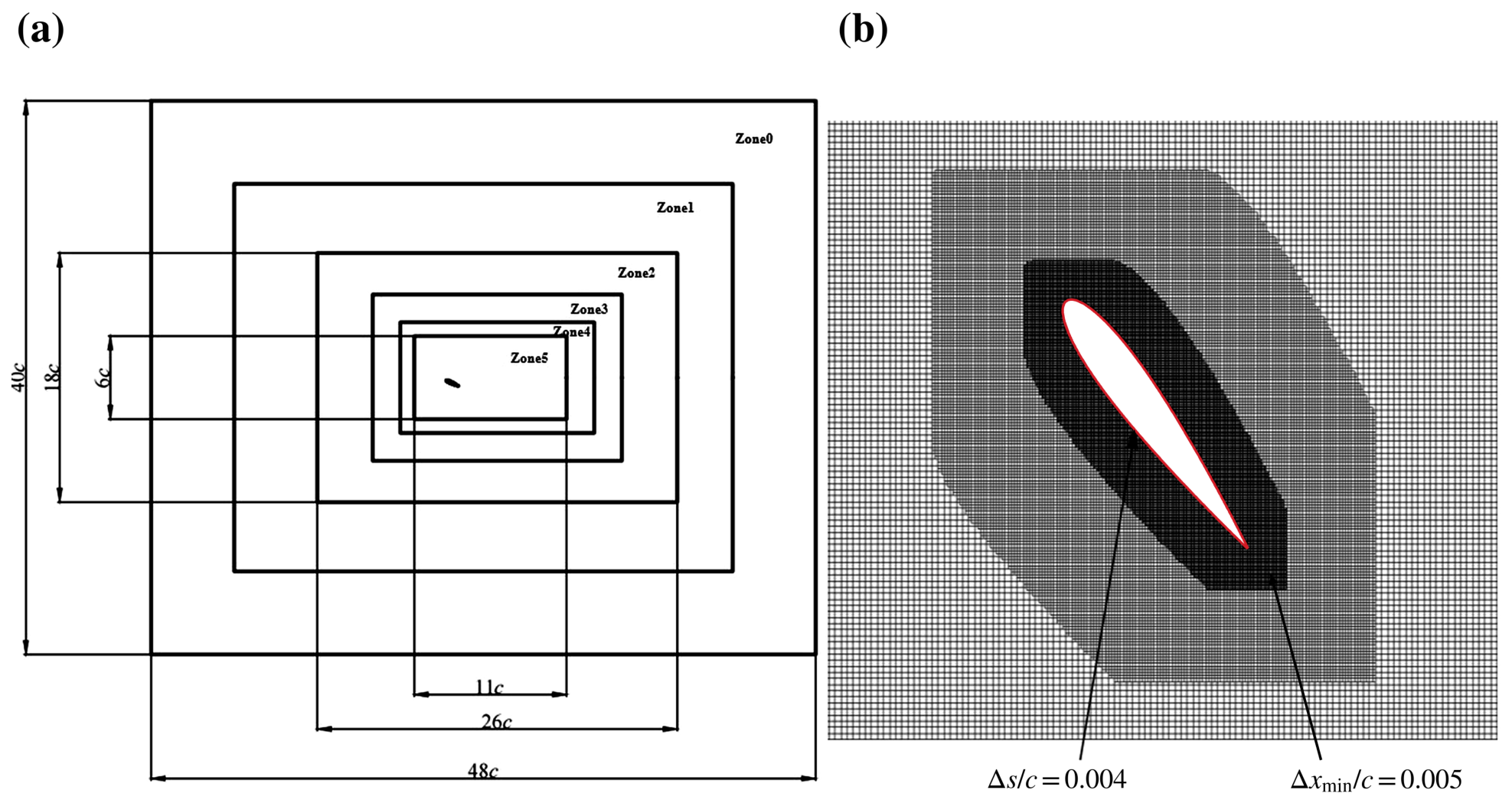
The MRT, pIB, and geometry-adaptive multi-block methods are documented in previous studies [34,38,39]. The refinement layout follows the strategy illustrated in Figure 2 of Wu and Wang [30], but uses the enlarged domain and the grid settings specified above. Three assessments were performed: comparison with published no-gust results to check force and power evaluation, a three-grid study of the coupled encounter, and analytical verification of Taylor-vortex diffusion.
Appendix A.1. Consistency with Published Flapping-Foil Results
For the no-gust configuration, the present calculation gives and (Table A1). Relative to Wu and Wang [30], the deviations are for and for . Relative to Kinsey and Dumas [7], the corresponding deviations are and . The largest deviation is . This level of agreement supports the consistency of the moving-boundary force and power evaluation. The published calculations use different numerical arrangements and averaging procedures. The comparison is therefore used as an external consistency check.
Table A1.
Comparison of the no-gust flapping-foil performance with published results.
Appendix A.2. Grid Sensitivity of the Coupled Encounter
Spatial-resolution sensitivity was assessed for the prescribed encounter defined by , , , and . The coarse, medium, and fine grids employed minimum Eulerian spacings of , , and , respectively, with the Lagrangian spacing refined concurrently. All physical parameters, boundary conditions, the encounter definition, and the sampling interval were held fixed across the three grids. Table A2 summarizes the resulting response quantities. Here, and denote the global maxima of and , respectively, over the nominal-encounter-aligned cycle, .
Table A2.
Grid-sensitivity results for the prescribed encounter at . All response quantities were evaluated over the nominal-encounter-aligned cycle, . Here, and denote the global maxima of and within this interval, respectively, while and denote the numbers of Eulerian nodes and Lagrangian points.
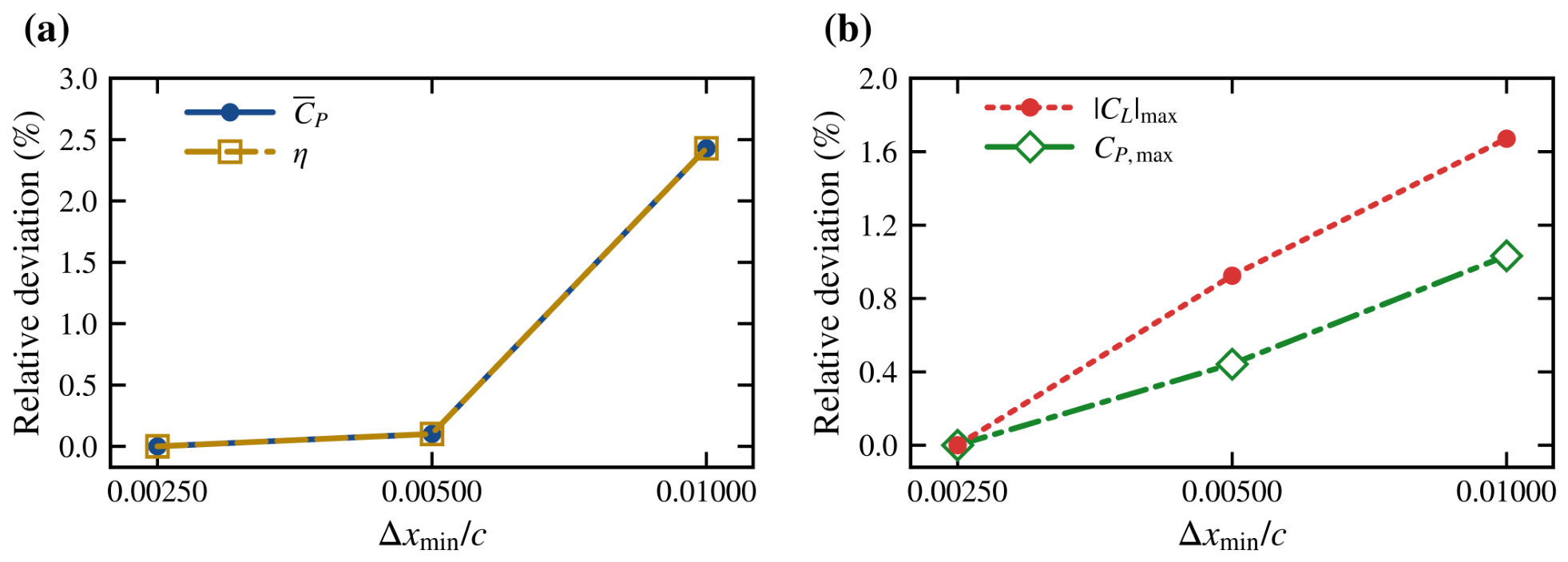
The prescribed kinematics fix , so the relative deviations of and are identical before rounding. Using the fine grid as the reference, the medium-grid deviations in , , and are , , and , respectively. The corresponding coarse-grid deviations are , , and . The response quantities do not converge monotonically in every case. Richardson extrapolation and the grid convergence index (GCI) are not reported for this coupled data set. Figure A2 presents these deviations relative to the fine-grid values.
The largest absolute relative deviation of the medium-grid result from the fine-grid reference is , while the deviations in and are both . Relative to the fine grid, the medium grid contains fewer Eulerian nodes and fewer Lagrangian points. Because the medium-grid deviations remain below for , , , and , the medium grid was retained for the subsequent production simulations.
Figure A2.
Spatial-resolution sensitivity of the prescribed encounter. Absolute relative deviations from the fine-grid values are shown for (a) the cycle-averaged power coefficient and hydrodynamic efficiency , and (b) the maximum absolute lift coefficient and maximum instantaneous power coefficient over the nominal-encounter-aligned cycle, .
Appendix A.3. Isolated Taylor-Vortex Diffusion Verification
Vortex diffusion was verified independently of the foil in a quiescent periodic domain, with no immersed-boundary forcing. For the Taylor-vortex profile used by Martínez-Muriel and Flores [17], the analytical viscous evolution is
Here, denotes the initial characteristic velocity scale corresponding to in Equation (4); the initial peak tangential speed is . For this diffusion test, , , and . The three uniform grids contain , , and points. Their respective spacings are , , and . The time step and shear-mode relaxation rate were adjusted to preserve the same physical viscosity. The full-field relative error is defined as
The numerical solution reproduces the analytical broadening and decay (Figure A3).
Figure A3.
Isolated Taylor-vortex diffusion. (a) Normalized velocity profiles at , 2, and 4; lines and open symbols denote the analytical and fine-grid solutions, respectively. (b) Peak-velocity magnitude. (c) Peak-radius location.
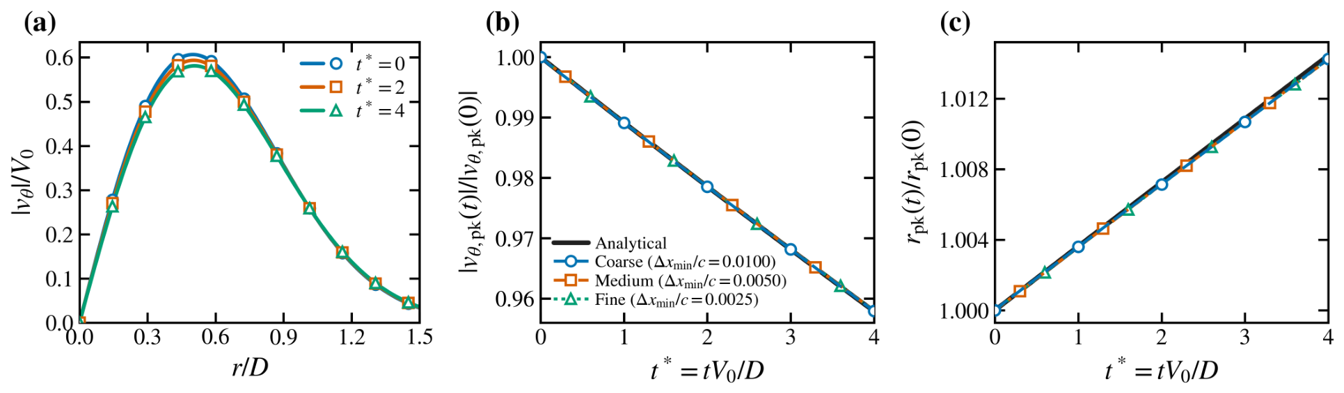
At , the fine-grid deviations in peak velocity, peak radius, and center vorticity are below . Over , the maximum full-field error is . The monotonically convergent diagnostics were used to calculate the observed convergence orders and GCI values, with a refinement ratio of and a safety factor of . The observed orders range from to . The maximum fine-grid is . The weak grid dependence of the error may reflect the difference between the periodic computational domain and the unbounded analytical solution.
The no-gust comparison checks the moving-boundary force and power evaluation against published results. The coupled grid study quantifies the spatial-resolution sensitivity of the complete encounter. The analytical diffusion test examines the viscous evolution of the imposed Taylor vortex. No available reference configuration matches all present kinematic and vortex parameters. These checks do not constitute a one-to-one validation of the complete moving-foil encounter. They provide evidence for the accuracy of its principal numerical components under the stated two-dimensional conditions.
References
- Olabi, A.G.; Abdelkareem, M.A. Renewable Energy and Climate Change. Renew. Sustain. Energy Rev. 2022, 158, 112111. [Google Scholar] [CrossRef] [Scilit]
- Lewis, M.; Neill, S.P.; Robins, P.E.; Hashemi, M.R. Resource Assessment for Future Generations of Tidal-Stream Energy Arrays. Energy 2015, 83, 403–415. [Google Scholar] [CrossRef] [Scilit]
- McKinney, W.; DeLaurier, J. Wingmill: An Oscillating-Wing Windmill. J. Energy 1981, 5, 109–115. [Google Scholar] [CrossRef] [Scilit]
- Young, J.; Lai, J.C.S.; Platzer, M.F. A Review of Progress and Challenges in Flapping Foil Power Generation. Prog. Aerosp. Sci. 2014, 67, 2–28. [Google Scholar] [CrossRef] [Scilit]
- Xiao, Q.; Zhu, Q. A Review on Flow Energy Harvesters Based on Flapping Foils. J. Fluids Struct. 2014, 46, 174–191. [Google Scholar] [CrossRef] [Scilit]
- Moriche, M.; Flores, O.; García-Villalba, M. On the Aerodynamic Forces on Heaving and Pitching Airfoils at Low Reynolds Number. J. Fluid Mech. 2017, 828, 395–423. [Google Scholar] [CrossRef] [Scilit]
- Kinsey, T.; Dumas, G. Parametric Study of an Oscillating Airfoil in a Power-Extraction Regime. AIAA J. 2008, 46, 1318–1330. [Google Scholar] [CrossRef] [Scilit]
- Zhu, Q.; Peng, Z. Mode Coupling and Flow Energy Harvesting by a Flapping Foil. Phys. Fluids 2009, 21, 033601. [Google Scholar] [CrossRef] [Scilit]
- Zhu, Q. Optimal Frequency for Flow Energy Harvesting of a Flapping Foil. J. Fluid Mech. 2011, 675, 495–517. [Google Scholar] [CrossRef] [Scilit]
- Young, J.; Ashraf, M.A.; Lai, J.C.S.; Platzer, M.F. Numerical Simulation of Fully Passive Flapping Foil Power Generation. AIAA J. 2013, 51, 2727–2739. [Google Scholar] [CrossRef] [Scilit]
- Liu, Z.; Bhattacharjee, K.S.; Tian, F.B.; Young, J.; Ray, T.; Lai, J.C.S. Kinematic Optimization of a Flapping Foil Power Generator Using a Multi-Fidelity Evolutionary Algorithm. Renew. Energy 2019, 132, 543–557. [Google Scholar] [CrossRef] [Scilit]
- Wu, X.; Zhang, X.; Tian, X.; Li, X.; Lu, W. A Review on Fluid Dynamics of Flapping Foils. Ocean Eng. 2020, 195, 106712. [Google Scholar] [CrossRef] [Scilit]
- Liu, Z.; Qu, H.; Song, X.; Chen, Z. A State-of-the-Art Review on Energy-Harvesting Performance of the Flapping Hydrofoil with Influential Parameters. Renew. Energy 2025, 245, 122849. [Google Scholar] [CrossRef] [Scilit]
- Jones, A.R.; Cetiner, O.; Smith, M.J. Physics and Modeling of Large Flow Disturbances: Discrete Gust Encounters for Modern Air Vehicles. Annu. Rev. Fluid Mech. 2022, 54, 469–493. [Google Scholar] [CrossRef] [Scilit]
- Hufstedler, E.A.L.; McKeon, B.J. Vortical Gusts: Experimental Generation and Interaction with Wing. AIAA J. 2019, 57, 921–931. [Google Scholar] [CrossRef] [Scilit]
- Alaminos-Quesada, J.; Fernández-Feria, R. Effect of the Angle of Attack on the Transient Lift during the Interaction of a Vortex with a Flat Plate: Potential Theory and Experimental Results. J. Fluids Struct. 2017, 74, 130–141. [Google Scholar] [CrossRef] [Scilit]
- Martínez-Muriel, C.; Flores, O. Analysis of Vortical Gust Impact on Airfoils at Low Reynolds Number. J. Fluids Struct. 2020, 99, 103138. [Google Scholar] [CrossRef] [Scilit]
- Barnes, C.J.; Visbal, M.R. Counterclockwise Vortical-Gust/Airfoil Interactions at a Transitional Reynolds Number. AIAA J. 2018, 56, 2540–2552. [Google Scholar] [CrossRef] [Scilit]
- Barnes, C.J.; Visbal, M.R. Angle of Attack and Core Size Effects on Transitional Vortical-Gust–Airfoil Interactions. AIAA J. 2020, 58, 2881–2898. [Google Scholar] [CrossRef] [Scilit]
- Qian, Y.; Wang, Z.; Gursul, I. Interaction of Quasi-Two-Dimensional Vortical Gusts with Airfoils, Unswept and Swept Wings. Exp. Fluids 2022, 63, 124. [Google Scholar] [CrossRef] [Scilit]
- Fukami, K.; Smith, L.; Taira, K. Extreme Vortex-Gust Airfoil Interactions at Reynolds Number 5000. Phys. Rev. Fluids 2025, 10, 084703. [Google Scholar] [CrossRef] [Scilit]
- Lopez-Doriga, B.; Magaña Jones, A.R.; Taira, K. On the Effect of Airfoil Geometry on Extreme Vortex-Gust Encounters. J. Fluid Mech. 2026, 1037, A61. [Google Scholar] [CrossRef] [Scilit]
- Ribeiro, B.L.R.; Su, Y.; Guillaumin, Q.; Breuer, K.S.; Franck, J.A. Wake-Foil Interactions and Energy Harvesting Efficiency in Tandem Oscillating Foils. Phys. Rev. Fluids 2021, 6, 074703. [Google Scholar] [CrossRef] [Scilit]
- Ribeiro, B.L.R.; Franck, J.A. Prediction of Energy Harvesting Efficiency through a Wake–Foil Interaction Model for Oscillating Foil Arrays. J. Fluid Mech. 2024, 996, A46. [Google Scholar] [CrossRef] [Scilit]
- Handy-Cardenas, E.E.; Zhu, Y.; Breuer, K.S. Optimal Kinematics for Energy Harvesting Using Favourable Wake–Foil Interactions in Tandem Oscillating Hydrofoils. J. Fluid Mech. 2025, 1012, A23. [Google Scholar] [CrossRef] [Scilit]
- Ren, H.; Wang, L.; Young, J.; Tian, F.B. A Predictive Framework for Energy Harvesting Based on Four Canonical Modes of Vortex–Foil Interaction. J. Fluid Mech. 2026, 1034, A49. [Google Scholar] [CrossRef] [Scilit]
- Rockwood, M.; Medina, A. Controlled Generation of Periodic Vortical Gusts by the Rotational Oscillation of a Circular Cylinder and Attached Plate. Exp. Fluids 2020, 61, 65. [Google Scholar] [CrossRef] [Scilit]
- Oshkai, P.; Iverson, D.; Lee, W.; Dumas, G. Reliability Study of a Fully-Passive Oscillating Foil Turbine Operating in a Periodically-Perturbed Inflow. J. Fluids Struct. 2022, 113, 103630. [Google Scholar] [CrossRef] [Scilit]
- Liu, Z.; Tian, F.B.; Young, J.; Lai, J.C.S. Flapping Foil Power Generator Performance Enhanced with a Spring-Connected Tail. Phys. Fluids 2017, 29, 123601. [Google Scholar] [CrossRef] [Scilit]
- Wu, S.; Wang, L. Numerical Study on the Energy Harvesting Performance of a Flapping Foil with Attached Flaps. Processes 2024, 12, 1963. [Google Scholar] [CrossRef] [Scilit]
- Young, J.; Tian, F.B.; Liu, Z.; Lai, J.C.S.; Nadim, N.; Lucey, A.D. Analysis of Unsteady Flow Effects on the Betz Limit for Flapping Foil Power Generation. J. Fluid Mech. 2020, 902, A30. [Google Scholar] [CrossRef] [Scilit]
- Chen, S.; Doolen, G.D. Lattice Boltzmann Method for Fluid Flows. Annu. Rev. Fluid Mech. 1998, 30, 329–364. [Google Scholar] [CrossRef] [Scilit]
- Guo, Z.; Zheng, C.; Shi, B. Discrete Lattice Effects on the Forcing Term in the Lattice Boltzmann Method. Phys. Rev. E 2002, 65, 046308. [Google Scholar] [CrossRef] [Scilit] [PubMed]
- Tian, F.B.; Luo, H.; Zhu, L.; Liao, J.C.; Lu, X.Y. An Efficient Immersed Boundary–Lattice Boltzmann Method for the Hydrodynamic Interaction of Elastic Filaments. J. Comput. Phys. 2011, 230, 7266–7283. [Google Scholar] [CrossRef] [Scilit] [PubMed]
- Yu, D.; Mei, R.; Shyy, W. A Multi-Block Lattice Boltzmann Method for Viscous Fluid Flows. Int. J. Numer. Methods Fluids 2002, 39, 99–120. [Google Scholar] [CrossRef] [Scilit]
- Kim, Y.; Peskin, C.S. Penalty Immersed Boundary Method for an Elastic Boundary with Mass. Phys. Fluids 2007, 19, 053103. [Google Scholar] [CrossRef] [Scilit]
- Peskin, C.S. The Immersed Boundary Method. Acta Numer. 2002, 11, 479–517. [Google Scholar] [CrossRef] [Scilit]
- Wang, L.; Tian, F.B. Numerical Simulation of Flow over a Parallel Cantilevered Flag in the Vicinity of a Rigid Wall. Phys. Rev. E 2019, 99, 053111. [Google Scholar] [CrossRef] [Scilit] [PubMed]
- Xu, L.; Tian, F.B.; Young, J.; Lai, J.C.S. A Novel Geometry-Adaptive Cartesian Grid Based Immersed Boundary–Lattice Boltzmann Method for Fluid–Structure Interactions at Moderate and High Reynolds Numbers. J. Comput. Phys. 2018, 375, 22–56. [Google Scholar] [CrossRef] [Scilit]

Disclaimer/Publisher’s Note: The statements, opinions and data contained in all publications are solely those of the individual author(s) and contributor(s) and not of MDPI and/or the editor(s). MDPI and/or the editor(s) disclaim responsibility for any injury to people or property resulting from any ideas, methods, instructions or products referred to in the content. |
© 2026 by the authors. Licensee MDPI, Basel, Switzerland. This article is an open access article distributed under the terms and conditions of the Creative Commons Attribution (CC BY) license.