A Numerical–Textual Dual-Channel Forecasting Framework for Short-Term Load Forecasting

Abstract

Short-term load forecasting underpins power-system dispatching, yet classical models degrade when historical samples are scarce. This paper proposes NTSForecast, a numerical–textual dual-channel framework: a trainable multi-layer perceptron encodes the numerical input, a frozen large language model (LLM) embeds the task instruction and the field labels, and a small head returns the load from the frozen decoder output. No backbone parameter is updated at any point. At each of six rolling origins training sees only a seven-day record of 94 samples, while the non-overlapping test windows supply 7824 held-out hourly points across four seasons, five seeds each. NTSForecast attains the lowest MAE, RMSE and MAPE of the methods compared (5.66 ± 0.04% against 5.68% for the strongest baseline), but that margin is small and sensitive to how serial dependence is handled; under scarce history the framework is competitive with that baseline, not superior to it. What the evidence does establish is the contribution of the frozen backbone. With architecture, trainable-parameter count, hyperparameters and data held identical, removing it costs 1.38 percentage points of MAPE. Backbone scale runs against a capacity argument; on a 0.5B-to-8B ladder the smallest pretrained backbone is the most accurate and becomes the reference configuration (1445 MB peak memory). Removing the textual channel costs 1.17 percentage points.

1. Introduction

Short-term load forecasting (STLF) aims to predict the load curve for the next several hours to the following day and directly serves unit commitment, economic dispatch, and demand-side management [1]. With the large-scale integration of distributed energy resources, the load fluctuations observed at the distribution-station level have become increasingly pronounced, and the dependence on meteorological factors has also grown [2]. These trends create two distinctive challenges for load forecasting: (i) the available samples at a target station area are typically scarce, which is particularly evident after topology renovation or the commissioning of a new substation; and (ii) the joint distribution of weather and load undergoes seasonal drift, so that a model that performs well in one season often loses accuracy after the seasonal switch.

Classical STLF methods can be grouped into three families: statistical models, represented by ARIMA and Holt–Winters [3]; shallow machine-learning methods such as support vector regression (SVR) [4] and gradient-boosting decision trees (GBDTs) [5]; and deep models such as LSTM [6], Transformer [7], DLinear [8], and PatchTST [9]. Such methods describe time-series regularities through parameterized functions but contain no information outside the training set; their ability to adapt to new scenarios therefore degrades noticeably when samples are scarce or when the distribution shifts.

Large language models (LLMs) introduce a new kind of usable prior for time-series forecasting. The pre-training corpora of LLMs cover vast amounts of physical common sense, calendar regularities, and economic knowledge, which can be transferred to forecasting tasks through prompt engineering [10], in-context learning [11], or lightweight fine-tuning such as LoRA [12]. Existing LLM-based forecasting methods, such as PromptCast [13], LLMTime [14], and GPT4TS [15], generally adopt a text-based input that serializes numerical values into tokens. This design requires the model to infer numerical magnitudes from character tokens, which is computationally expensive and accuracy-limited in long-horizon forecasting. Another family of approaches focuses on the numerical channel: a small projection layer maps the numerical sequence into the embedding space of the LLM, while the LLM body remains frozen. This design substantially reduces the training cost, but using only a single numerical modality forfeits the contextual information carried by the task text.

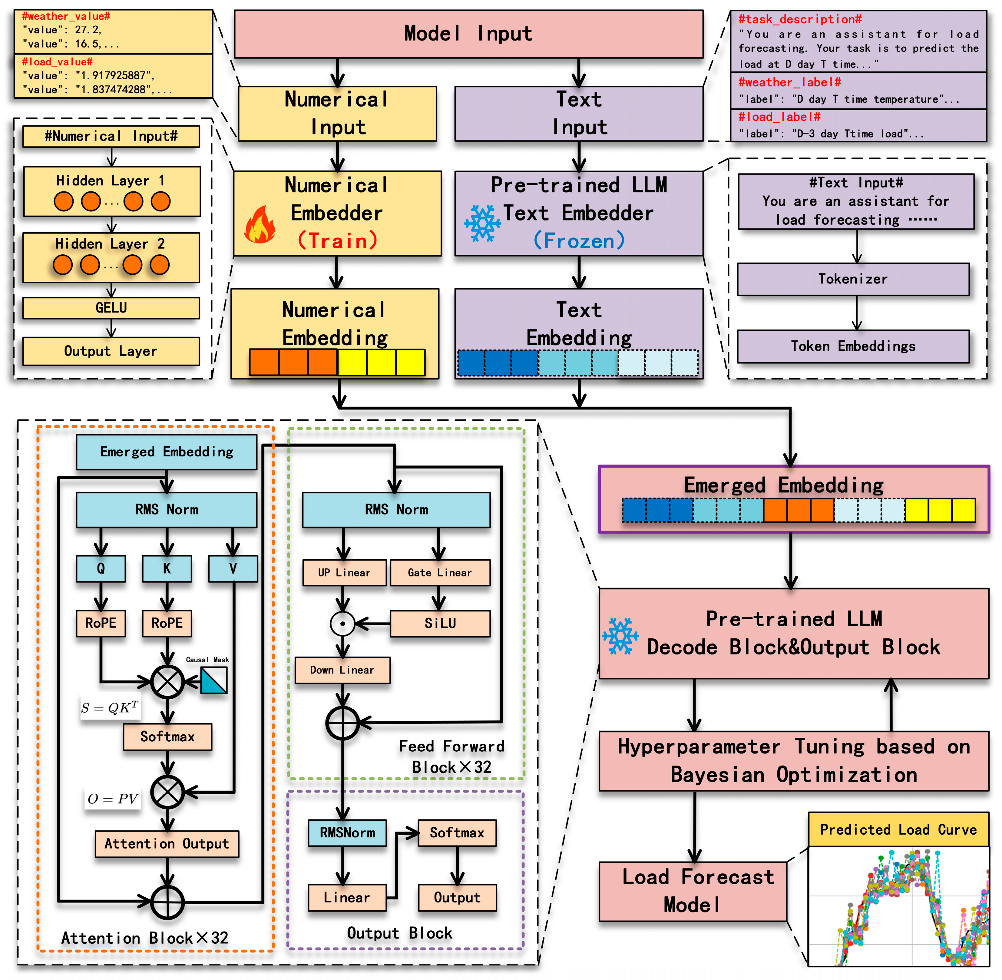
This paper proposes NTSForecast. A trainable multi-layer perceptron projects each numerical field into the hidden space of a frozen language model, a frozen text encoder embeds the task instruction and the field labels, and the two sets of embeddings are concatenated along the sequence dimension and passed through the frozen decoder, from which a lightweight regression head returns the load. No backbone parameter is updated at any point, layer normalization and positional embeddings included, whereas comparable frozen-backbone methods adapt both. The reference configuration uses the frozen Qwen2.5-0.5B decoder; Section 6.6 compares it with a randomly initialized backbone, Qwen2.5-1.5B and Llama-3.1-8B [16] under identical settings, where accuracy runs opposite to backbone size. Multimodal fusion in itself is not the claim: compact multimodal forecasters such as the CNN–LSTM day-ahead price model of [17] establish that premise without a language model. One qualification belongs with the architecture. The text channel is load-bearing, but on this dataset, it carries a fixed instruction and a set of field labels that are identical in every sample, so its contribution is not semantic.

The main contributions of this paper are summarized as follows:

(1) A “frozen backbone + trainable numerical channel” dual-modal architecture tailored to short-term load forecasting, in which multimodal fusion is completed without updating any parameter of the language model, including its layer-normalization and positional-embedding parameters. A controlled comparison measures what the frozen backbone contributes: on the HEEW dataset removing the frozen backbone raises MAPE by 1.38 percentage points (7.0374 without it versus 5.6621 with it; Welch t-test on per-seed MAPE, p = 0.0038). Since the two variants share architecture, trainable-parameter count, hyperparameters and data, that difference belongs to the frozen backbone and not to capacity or tuning. Against the full comparison set the framework attains the lowest error on all three scale-dependent and relative metrics, though the margin over the strongest baseline is small, and its significance depends on how serial dependence is handled (Section 6.2). The evidence has three limits: one region and one deployment year, a margin over the strongest baseline of a fraction of a percentage point in MAPE, and no gain from larger backbones. Section 6.2 gives the full ordering, Section 6.8 the per-origin breakdown, and Section 7 the boundary of the claim.

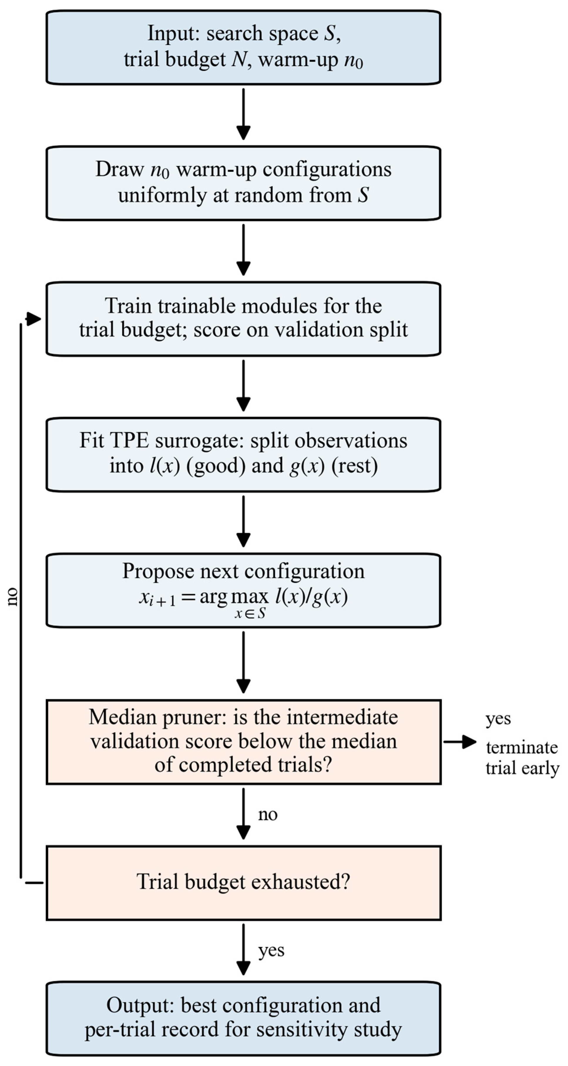
(2) A Bayesian-optimization procedure for the full model: with the LLM backbone fixed, we jointly search a five-dimensional hyperparameter space and tune directly against the validation MAPE, only training the learnable modules.

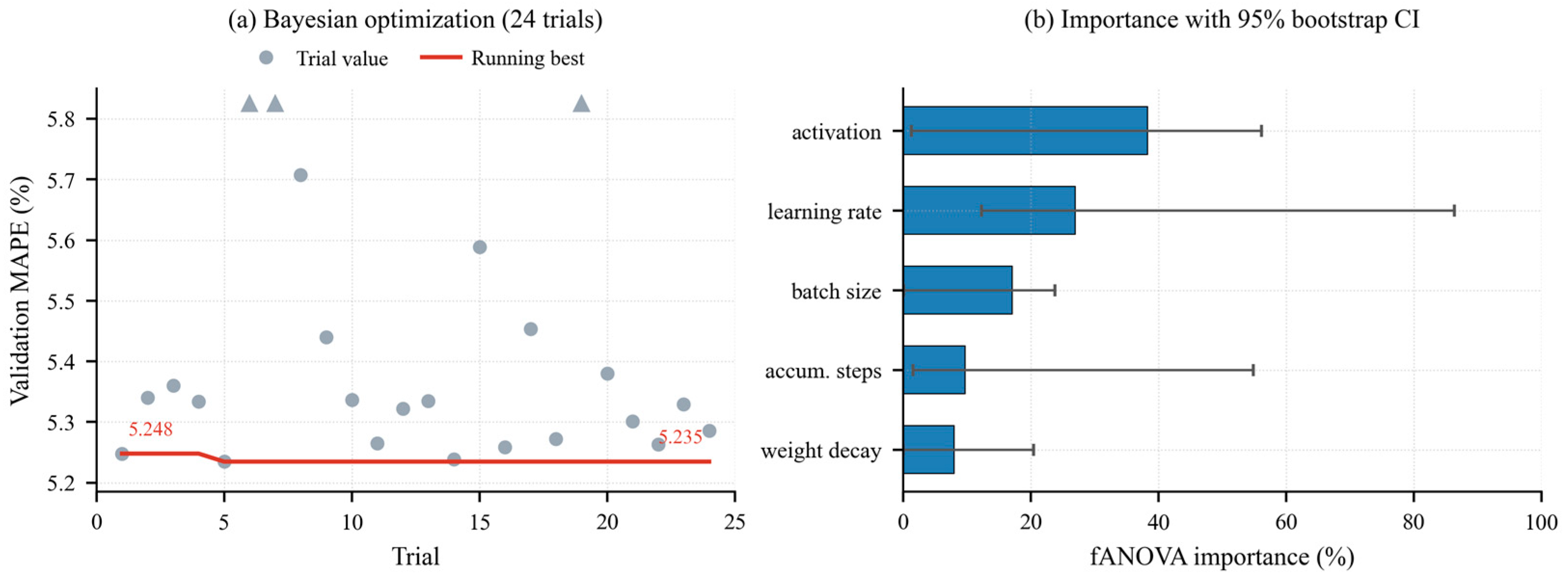
(3) A hyperparameter sensitivity study of the resulting configuration. We apply fANOVA to decompose the validation objective across the searched hyperparameters, and we report the result together with bootstrap confidence intervals over the optimization trials. Those intervals overlap for all five hyperparameters at the trial budget used here, so no importance ranking is claimed; the analysis is reported as a sensitivity study, and Section 7.3 states what it does and does not establish. We include it because the trial budget required to obtain stable importance estimates is itself a practically relevant finding for work that tunes frozen-backbone forecasters.

The remainder of this paper is organized as follows. Section 2 describes the data and the feature construction. Section 3 develops the dual-channel architecture. Section 4 describes the Bayesian optimization and the fANOVA procedure. Section 5 defines the evaluation metrics. Section 6 reports the experimental results. Section 7 discusses the findings, and Section 8 concludes the paper.

2. Data and Feature Construction

2.1. Data Source

The evaluation uses the region-level aggregate of the publicly available HEEW dataset (Hierarchical Energy, Emissions and Weather) [18], which records hourly electricity consumption and synchronous meteorological observations for the Arizona State University campuses (Arizona, USA) under a CC-BY 4.0 licence; the meteorological variables are reported in the source units of the dataset (°F, inHg). The forecast target is the electricity channel of that dataset, which the source distributes in kilowatts and which is expressed in megawatts throughout this paper (1 MW = 1000 kW); the total-energy channel, which the source reports in mmBtu after aggregating electricity, cooling and heat, is not used.

The source covers 2014 to 2022 at hourly resolution. This study uses the 9294 consecutive hours from 9 December 2018 to 31 December 2019. The series is gap-free over that window, so the rule that removes records affected by communication outages or obvious anomalies discards nothing, and every hour enters the protocol below. For each forecast time slot, a sample pairs the three meteorological variables retained by the screening of Section 2.2 with nine historical load lags: the load at the forecast slot and at one and two slots earlier on each of the three preceding days. The window is split strictly chronologically at six rolling origins. Each origin trains on a seven-day raw record. The lags reach back three days and two hours, so the last 94 of its 168 h form complete training samples; the following 1302 h form the validation window and the next 1304 h the held-out test window. The three periods are contiguous, strictly ordered and disjoint, and the six test blocks are consecutive and non-overlapping, so they tile a 9 February 2019 to 31 December 2019 record of 6 × 1304 = 7824 hourly points across all four seasons, and every hour of the study window is used exactly once as a test hour. The origins sit about 54 days apart, so neighbouring ones draw on overlapping history and only the six test blocks are disjoint. Each origin is retrained from scratch and tested strictly after its own training and validation periods.

The seven-day training record is a deliberate choice rather than a shortage: feeders that have just been commissioned, reconnected or reconfigured often have no more than a week of history. Training on a week while evaluating on a full year reproduces that situation without making the assessment itself small.

2.2. Correlation Analysis of Meteorological Covariates

Meteorological inputs are selected with five screening criteria instead of the Pearson correlation alone. The load–temperature relationship is nonlinear and mediated by comfort, so a linear coefficient on its own cannot settle whether a variable belongs in the input. What drives cooling and heating demand is occupant thermal comfort, which responds to thresholds and saturates as ambient conditions change [19]. A variable can therefore drive load strongly and still show a near-zero linear coefficient. We report the absolute Pearson correlation, the absolute Spearman rank correlation, mutual information, the Hilbert–Schmidt independence criterion (HSIC) and permutation importance, computed on the historical record preceding the validation period (feature screening uses no validation or test data). The candidate pool comprises temperature, relative humidity, wind speed, dew point and pressure. Temperature ranks first under all five criteria ($\left|r\right|$ = 0.657, $\left|\rho \right|$ = 0.690, MI = 0.379, HSIC = 0.036, permutation importance = 0.709), followed by dew point (0.539, 0.485, 0.221, 0.014, 0.324) and pressure; relative humidity and wind speed rank at the bottom under every criterion, and the permutation importance of humidity is not distinguishable from zero. The three retained exogenous covariates are therefore temperature, dew point and pressure. Temperature is used by the model in every experiment reported in this manuscript. Figure 1 summarises the screening.

2.3. Autocorrelation Structure of the Load Series

Figure 2 shows the autocorrelation function (ACF) of the hourly load series over the contiguous evaluation block. Pronounced peaks appear at lag 24 (one full day, ACF = 0.884) and at lag 48 (two days, ACF = 0.802), and the weekly cycle is equally visible (lag 168, ACF = 0.801). This strong daily periodicity motivates the historical-load features of

Table 1. Input fields of one complete sample, exactly as presented to the model. Three meteorological variables and nine historical load lags form the 12-dimensional input; the target is the load at the forecast slot. D denotes the forecast day and T the forecast time slot.

Category	Field Label (as Presented to the Model)	Unit	Example Value
Meteorological variable	D day T time temperature	°F	91
	D day T time dew point	°F	38
	D day T time pressure	inHg	28.66
Historical load	D-3 day T-2 h load	MW	31.07357
Historical load	D-3 day T-1 h load	MW	32.19715
Historical load	D-3 day T load	MW	32.55978
Historical load	D-2 day T-2 h load	MW	30.97558
Historical load	D-2 day T-1 h load	MW	32.2129
Historical load	D-2 day T load	MW	33.24257
Historical load	D-1 day T-2 h load	MW	30.11902
Historical load	D-1 day T-1 h load	MW	30.87537
Historical load	D-1 day T load	MW	31.16313
Prediction target	D day T time load	MW	27.82631

—the same hour and its two predecessors on each of the three preceding days—and it also fixes the reference that every learned model must beat: a naive forecast that repeats the previous day’s load at the same hour already captures most of this structure.

2.4. Sample Format of the Dual-Channel Model

Each sample is organized as a JSON object with four parts: a task description, three meteorological variables, nine historical load lags, and the target value. The numerical fields are fed to the numerical channel; the task description and the field labels enter the frozen text encoder. Section 2.1 gives the chronological three-way split used at each of the six rolling origins. Two points follow from it for the samples described above. Because the feature representation reaches back 74 h, only the last 94 h of a seven-day record form complete input–target pairs, and the construction checks sample by sample that no lag feature reaches outside that record. Epoch selection and every other model-selection decision use the validation window alone, and the held-out block is evaluated once. Table 1 lists the input fields of a complete sample with example values. The labels inherit the naming used in the JSON file: D denotes the forecast day and T the forecast time slot, so that “D-1 day T load” is the load at the same time slot on the previous day.

3. Numerical–Textual Dual-Channel Architecture

3.1. Overall Framework

The overall architecture of NTSForecast is shown in Figure 3. It consists of five main modules: (i) a trainable numerical encoder that maps the 12-dimensional input vector to a hidden vector whose dimension matches the LLM token embedding space; (ii) a frozen pretrained LLM text encoder that projects the task instruction into the same hidden space; (iii) a fusion module that concatenates the two outputs along the sequence dimension; (iv) a frozen pretrained LLM decoder that performs self-attention on the concatenated sequence; and (v) a lightweight regression head that maps the last hidden state to a scalar load prediction. The Bayesian-optimization module on the right of the figure is separate from the forward path and is responsible for determining the hyperparameters of the numerical encoder. It should be emphasized that the LLM text encoder and decoder are fully frozen during training (snowflake markers); only the numerical encoder and the regression head receive gradient updates (flame markers). The training cost is therefore much lower than that of a full-parameter fine-tuning scheme.

3.2. Trainable Numerical Encoder

Let $x\in R^{12}$ denote the standardized input vector. The numerical encoder is implemented as an L-layer MLP with an element-wise nonlinear activation:

$$h^{\left(l\right)}=\sigma \left(W_l{h}^{(l-1)}+b_l\right),l=1,\dots ,L$$

(1)

The above output is then fed into the frozen text-encoder side as a token-like embedding sequence.

$$e_{num}=W_{proj}{h}^{\left(L\right)}+b_{proj}$$

(2)

3.3. Frozen Text Encoder

The task instruction t (a fixed natural-language prompt that declares the forecasting target) is tokenized into a sequence of length T. The frozen text encoder maps it to token embeddings:

$$E_{txt}=f_{LLM}\left(t\right)$$

(3)

where $f_{LLM}$ is the embedding layer of the pretrained LLM, whose weights remain frozen throughout training. This design preserves the semantic information learned during pre-training and avoids catastrophic forgetting during fine-tuning.

3.4. Fused Embedding and Frozen Decoder

The numerical embedding and the text embeddings are concatenated along the sequence dimension to obtain a fused embedding sequence:

$$E=\left[e_{num};E_{txt}\right]$$

(4)

which is then fed to the decoder module of the pretrained LLM. The weights of this module are frozen in both training and inference phases, and the module only acts as a “context understanding” component, so that there is no risk of catastrophic forgetting caused by a small-sample task. Let $g_{LLM}$ denote the forward operator of the frozen decoder, and take the hidden state of the last token as the sequence summary:

$$z=g_{LLM}{\left(E\right)}_{\left[last\right]}$$

(5)

3.5. Regression Head and Training Objective

The hidden state z is mapped to the scalar load prediction by a lightweight regression head (a two-layer MLP):

$$\hat{\mathrm{y}}=W_2\sigma \left(W_{1}z+b_1\right)+b_2$$

(6)

During training, the trainable parameter set $\theta$ only comprises the numerical-encoder weights $(W_l,b_l,W_{proj},b_{proj})$ and the regression-head weights $(W_1,b_1,W_2,b_2)$. The loss function is the mean squared error augmented with an L2 regularization term:

$$\mathcal{L}={\displaystyle \frac{1}{N}}{\displaystyle \sum _{i=1}^N}{\left({\hat{\mathrm{y}}}_i-y_i\right)}^2+\lambda {\left(\Vert \theta \Vert \right)}^2$$

(7)

Because the language model is frozen, back-propagation updates only the numerical encoders and the regression head—1,841,793 parameters in total—and no optimizer state is maintained for the backbone. This is the source of the training-cost reduction relative to full-parameter or LoRA-style adaptation of the same backbone. We quantify the cost in Section 7.1 rather than asserting it here, and we note at the outset that the reduction applies to training only: the forward pass executes the full backbone in every case, so inference latency and peak memory are not reduced by freezing.

4. Bayesian Optimization and Hyperparameter Importance Analysis

4.1. Motivation

The accuracy of neural-network forecasters is highly sensitive to hyperparameters: model capacity, regularization strength, and optimizer choices can all significantly affect the final result. In a setting where each single training run is expensive, the computational cost of grid search grows exponentially with the dimensionality, and random search cannot leverage information from existing trials; both sample efficiencies are therefore unsatisfactory. Bayesian optimization (BO) performs the search in a sequential manner: a probabilistic surrogate of the objective function is fitted to the completed trials, and the next candidate is selected by maximizing an acquisition function [20]. BO has a high sample efficiency and is well suited to STLF tasks with relatively high per-run training cost.

4.2. Search Space

This section performs joint tuning of the five key hyperparameters directly on the full NTSForecast model. The search space is given in

Table 2. Hyperparameter search space for Bayesian optimization.

Hyperparameter	Range/Choices
learning rate	[1 × 10−5, 5 × 10−3] (log-scale)
weight decay	[1 × 10−5, 1 × 10−1] (log-scale)
batch size	{2, 4, 8}
accum steps	{1, 2, 4}
activation	{GELU, ReLU, tanh, sigmoid}

. The LLM backbone remains frozen; only the numerical embedder, the text projection, and the regression head are trained. Learning rate and weight decay are sampled on a logarithmic scale across their intervals to cover different orders of magnitude, while batch size, accum steps, and activation are categorical variables drawn with uniform priors. Batch size and accum steps together determine the effective gradient batch, and their ranges are chosen to cover effective batch sizes between two and 32 within a 48 GB memory budget. Activation is shared by the hidden layers of the numerical embedder and the load embedder.

4.3. TPE-Sampler-Based Bayesian Optimization

We use the Tree-structured Parzen Estimator (TPE) sampler, which fits two density estimators on the hyperparameter space: $l\left(x\right)$ describes the configurations whose objective value is below a quantile threshold, and $g\left(x\right)$ describes the rest. The next trial is selected by maximizing ${\displaystyle \frac{l\left(x\right)}{g\left(x\right)}}$, which is monotonically related to the Expected Improvement (EI) acquisition function, as given in Equation (8):

$$x_{i+1}=arg{max}_{x\in \mathcal{S}}{\displaystyle \frac{l\left(x\right)}{g\left(x\right)}}$$

(8)

The optimization follows the sequential model-based framework of [21], as implemented in Optuna [22], with the TPE sampler; the importance decomposition uses the variance-based sensitivity indices of [23]. Considering the cost of a full training run, the trial budget is set to N = 24 with the first n₀ = 4 random warm-up trials; each trial trains the learnable modules of NTSForecast for six epochs on the training subset and evaluates the MAPE on the validation subset. The held-out test subset is never used for trial scoring. To save computing further, a median pruner terminates unpromising trials early. As reported in Section 6.7, even this budget is too small to support stable importance rankings, and the analysis is presented as a sensitivity study only. Figure 4 sets out the procedure.

4.4. fANOVA-Based Importance Analysis

Given the BO trial history $H=\left\{\right(x_i,y_i\left)\right\}$, fANOVA orthogonally decomposes the objective-function variance into contributions from individual hyperparameters and their interactions [24]. The marginal importance of hyperparameter $x_k$ is defined as

$$I_k={\displaystyle \frac{{\mathrm{Var}}_{x_k}\left({\mathbb{E}}_{x_{\sim k}}\left[\widehat{f}\left(x\right)|x_k\right]\right)}{{\mathrm{Var}}_x\left(\widehat{f}\left(x\right)\right)}}$$

(9)

where $\widehat{f}$ is the random-forest surrogate fitted on H. The larger $I_k$ is, the more of the performance fluctuation is explained by $x_k$.

5. Evaluation Metrics

All five metrics used in this manuscript are defined in Equations (10)–(13), before their first use: $y$ denotes the observed load, $\widehat{y}$ the forecast, and $n$ the number of held-out test samples. MAE (10) is the mean absolute error, in the same unit as the load; MSE and its root RMSE (11) penalize large deviations more heavily than MAE. MAPE (12) is the mean absolute percentage error, and SMAPE (13) its symmetric variant, which is bounded and does not diverge as the observed load approaches zero. MAE and RMSE are scale-dependent and therefore comparable only within a dataset; MAPE and SMAPE are dimensionless and comparable across datasets.

$$MAE={\displaystyle \frac{1}{n}}{\displaystyle \sum _{i=1}^n}\left|{\widehat{y}}_i-y_i\right|$$

(10)

$$MSE={\displaystyle \frac{1}{n}}{\displaystyle \sum _{i=1}^n}{\left({\widehat{y}}_i-y_i\right)}^2,RMSE=\sqrt{MSE}$$

(11)

$$MAPE={\displaystyle \frac{100\%}{n}}{\displaystyle \sum _{i=1}^n}\left|{\displaystyle \frac{{\widehat{y}}_i-y_i}{y_i}}\right|$$

(12)

$$SMAPE={\displaystyle \frac{100\%}{n}}{\displaystyle \sum _{i=1}^n}{\displaystyle \frac{2\left|{\widehat{y}}_i-y_i\right|}{\left|{\widehat{y}}_i\right|+\left|y_i\right|}}$$

(13)

Because several of the differences reported in Section 6 are small relative to seed-to-seed variation, we test them rather than reading them off the tables. For two forecasts with error series e¹ and e², the loss differential and the Diebold–Mariano statistic are given in Equation (14), where $\widehat{V}$ denotes the long-run variance estimated from the autocovariances of the differential. For a one-step horizon we apply the Harvey–Leybourne–Newbold small-sample correction of Equation (15) with h = 1, and refer the corrected statistic to a t-distribution with $n-1$ degrees of freedom. A negative statistic indicates that the first forecast has the lower squared error. The test is computed per seed against the strongest baseline in the comparison set, and

Table 3. Comparison of NTSForecast against classical, deep, published LLM-based and zero-shot foundation-model forecasters on the held-out evaluation period (7824 hourly points). Learned models are reported as mean ± standard deviation over five random seeds. The last column tests each row against Chronos-Bolt-Base, the baseline with the lowest MAPE, by the Diebold–Mariano statistic of Equation (14), whose loss is the squared error: a negative value favours the row, and n/N counts the seeds, out of those run, at which the row is significantly better at the 5% level. A significant difference in the opposite direction therefore counts as zero. These statistics are re-estimated under wider bandwidths later in this section. The statistic is a t-ratio computed over the 7824 evaluation points, so its magnitude reflects how consistent a difference is, not how large it is; the size of a difference is given by the metric columns.

Model	MAE	RMSE	MAPE/%	SMAPE/%	DM vs. Strongest Baseline
Ridge regression	4.5926	6.3966	16.4762	19.1504	+43.27 (p < 0.0001, 0/1)
Random forest	3.7558	4.7590	13.9314	14.2221	+48.93 (p < 0.0001, 0/1)
Gradient-boosted trees	3.9052	5.0450	14.4249	14.8618	+47.22 (p < 0.0001, 0/1)
LSTM	15.3793 ± 0.2326	15.9156 ± 0.2250	56.3479 ± 0.8869	79.0527 ± 1.7183	+164.79 (p < 0.0001, 0/5)
GRU	15.2212 ± 0.4522	15.7619 ± 0.4362	55.7475 ± 1.7263	77.9277 ± 3.2754	+163.31 (p < 0.0001, 0/5)
Transformer encoder	12.4326 ± 0.2718	13.0874 ± 0.2581	45.1126 ± 1.0365	58.9986 ± 1.7102	+134.58 (p < 0.0001, 0/5)
DLinear	16.0893 ± 24.5869	16.7360 ± 24.6470	60.1021 ± 91.8243	52.7884 ± 74.2840	+99.75 (p < 0.0001, 0/5)
PatchTST	2.0278 ± 0.1383	2.6214 ± 0.1788	7.6149 ± 0.4920	7.5711 ± 0.5040	+19.27 (p < 0.0001, 0/5)
TimeMoE-50M (zero-shot)	1.5275	2.0706	5.7749	5.7500	−3.63 (p = 0.0003, 1/1)
Sundial-128M (zero-shot)	1.5652	2.1048	5.9186	5.8869	−0.32 (p = 0.7491, 0/1)
Chronos-Bolt-Base (zero-shot)	1.5044	2.1087	5.6772	5.6858	reference
Parameter-matched MLP	1.8333 ± 0.1071	2.3173 ± 0.1345	7.0374 ± 0.4624	6.9066 ± 0.3498	+8.50 (p = 0.0012, 0/5)
GPT4TS	1.6952 ± 0.0317	2.2016 ± 0.0290	6.4829 ± 0.1327	6.3895 ± 0.1314	+4.57 (p = 0.0107, 0/5)
Time-LLM	1.5469	2.0749	5.8491	5.8064	−2.13 (p = 0.0334, 1/1)
NTSForecast (proposed)	1.4926 ± 0.0113	2.0672 ± 0.0071	5.6621 ± 0.0448	5.6105 ± 0.0448	−4.17 (p = 0.0002, 5/5)

reports both the mean statistic and the number of seeds at which the difference is significant at the 5% level.

$$d_i={\left({e^1}_i\right)}^2-{\left({e^2}_i\right)}^2,DM={\displaystyle \frac{\overline{d}}{\sqrt{\widehat{V}\left(\overline{d}\right)}}}$$

(14)

$${DM}_{HLN}=DM·\sqrt{{\displaystyle \frac{n+1-2h+\frac{h(h-1)}{n}}{n}}}$$

(15)

Computational environment. All experiments were run on a single NVIDIA RTX A6000 (48 GB) under Ubuntu, with Python 3.10 and PyTorch 2.9.1 (CUDA 12.8 build). The frozen backbone is loaded through the HuggingFace Transformers library. Bayesian optimization uses Optuna with the TPE sampler and a median pruner. The comparison methods use the implementations released by their authors: GPT4TS and PatchTST from the official One-Fits-All repository, Time-LLM through the NeuralForecast library, and TimeMoE, Sundial and Chronos-Bolt from the published model weights; the classical baselines use scikit-learn. Random seeds, library versions and the single hyperparameter configuration used throughout are listed in Section 6.1 so that the results can be reproduced.

6. Experiments and Results

6.1. Experimental Setup

All baselines and the proposed method use the same 12-dimensional input and the same chronological three-way split at every origin. The backbone of the reference configuration is the frozen Qwen2.5-0.5B model loaded in float16; all of its weights remain frozen, and no LoRA or other adaptation is applied. The backbone-scale study of Section 6.6 compares this configuration with a randomly initialized backbone and with frozen Qwen2.5-1.5B and Llama-3.1-8B backbones under identical settings; the 0.5B configuration is used as the reference throughout because it is the most accurate of the four on this task and has the smallest seed-to-seed spread. The numerical encoders and the regression head contain 1,841,793 trainable parameters in total. Optimization uses AdamW with the configuration located by the Bayesian optimization of Section 4, run on the reference configuration and scored on the validation split only: learning rate 3.35 × 10⁻³, weight decay 2.05 × 10⁻⁵, batch size two with one gradient-accumulation step, and ReLU activation. This single configuration carries over unchanged to the full model and to every ablation and backbone-scale variant, so no variant receives tuning of its own. Each configuration is trained with five random seeds, and all results are reported as mean ± standard deviation. The validation subset governs early stopping. The held-out test subset is evaluated once, after training is complete.

6.2. Comparison Against Mainstream Baselines

Table 3 reports the four metrics on the held-out test set. All baselines are retrained under the same protocol as the proposed method. The recurrent baselines follow the residential and multi-source load-forecasting settings of [25,26]; the institutional-building study of [27] is the closest published setting to the campus load studied here; and the attention-based baselines follow [28,29,30], with the general sensitivity of recurrent architectures to distribution drift discussed in [31] and the broader survey of attention models for time series in [32]. The comparison set includes three classical regressors (ridge regression, random forest and gradient-boosted trees), three sequence baselines (LSTM, GRU and a Transformer encoder), the published linear and patch-based baselines DLinear [8] and PatchTST [9], the published implementations of GPT4TS [15] and Time-LLM [33], three domain-specific time-series foundation models evaluated zero-shot—TimeMoE-50M [34], Sundial-128M [35] and Chronos-Bolt-Base [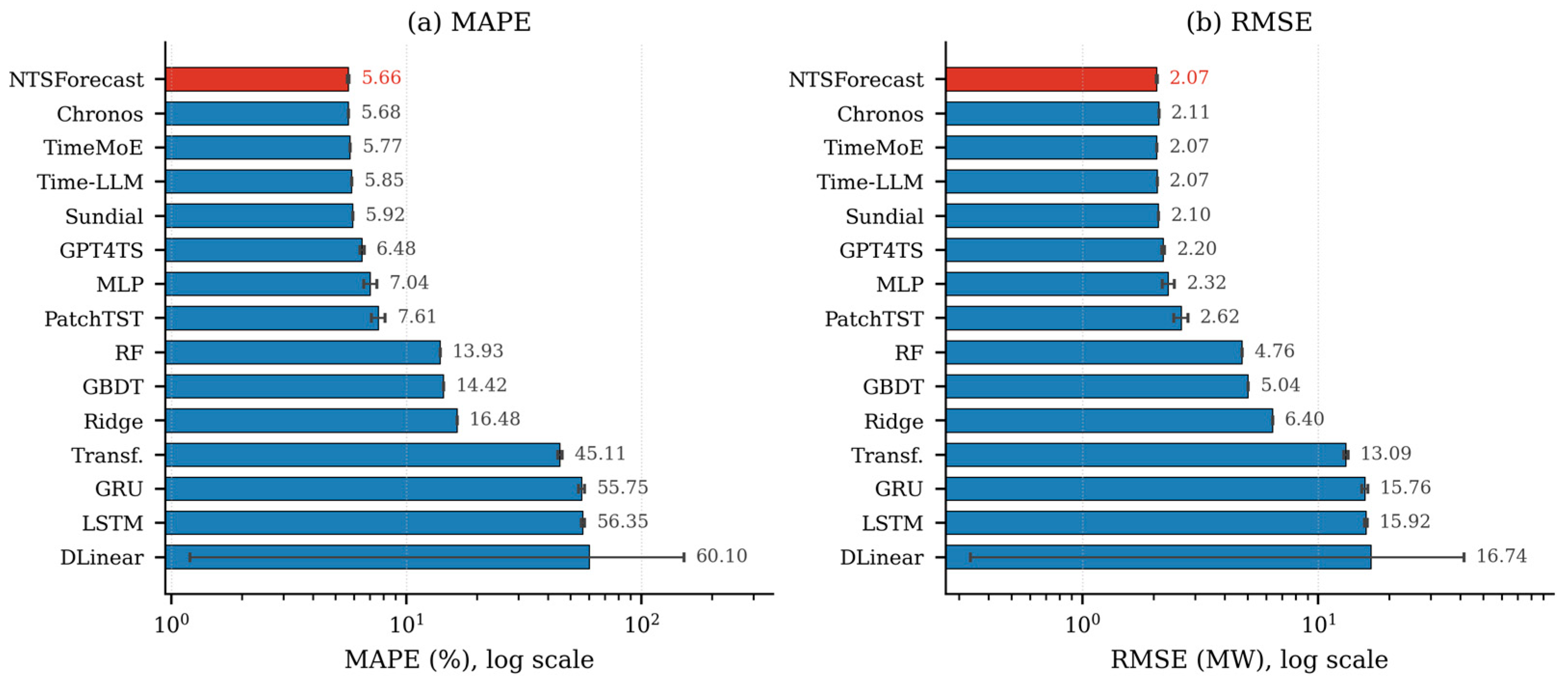36]—and a numerical encoder matched to NTSForecast in architecture and trainable-parameter count but with the backbone removed. NTSForecast attains MAE = 1.4926 ± 0.0113, RMSE = 2.0672 ± 0.0071 and MAPE = 5.6621 ± 0.0448, the lowest value of each in the table. The strongest baseline is Chronos-Bolt-Base applied zero-shot at 5.6772 MAPE, and the Diebold–Mariano test against it favours the proposed framework (DM = −4.17, p = 0.0002, with the difference significant at the 5% level for five of the five seeds).

Every significance statement in this paper is computed per seed and summarized as mean ± standard deviation across seeds. Seed-averaged ensemble forecasts are not reported, since averaging across seeds yields a predictor that was never trained and flatters every multi-seed method against the single-run baselines. The loss in the Diebold–Mariano test of Equation (14) is the squared error, the same loss the models are trained on (Equation (7)); the ordering of the table is by MAPE. The two need not agree, and here they do not: TimeMoE and Time-LLM reach a lower squared error than Chronos-Bolt-Base while their MAPE is higher, which is why the test can favour a row whose MAPE is worse than the reference. NTSForecast ranks first under both losses (MAE 1.4926 ± 0.0113, RMSE 2.0672 ± 0.0071, MAPE 5.6621 ± 0.0448), so the choice of loss does not decide the comparison that matters here.

A one-step loss differential is serially uncorrelated only when the forecasts are optimal, so the zero-lag bandwidth of Equation (15) is worth checking rather than assuming. Re-estimating the long-run variance with a Bartlett kernel leaves the direction unchanged and the magnitude smaller: against the strongest baseline the statistic is −2.42 at the automatic Newey–West bandwidth (p = 0.0362, significant for 3/5 seeds) and −2.10 at a bandwidth spanning a full daily cycle (p = 0.0660). The margin thus holds under the automatic bandwidth and is marginal under the daily-cycle bandwidth. For that reason, this paper describes the framework as competitive with the strongest baseline rather than superior to it.

Table 3 falls into three bands, and that separation is the main empirical finding of this paper. Methods that must learn the load–weather mapping from the 94 in-window samples without a pretrained prior collapse: the recurrent and attention sequence models exceed 45% MAPE, and the classical regressors reach 13.9314 (random forest) and 16.4762 (ridge). A middle band carries a prior but does not draw on it fully at this sample size: PatchTST (7.6149 ± 0.4920), the parameter-matched MLP (7.0374 ± 0.4624) and GPT4TS (6.4829 ± 0.1327). The leading band brings a large pretrained prior to a scarce training window: the three zero-shot foundation models (5.6772, 5.7749 and 5.9186), Time-LLM (5.8491) and NTSForecast, which is the most accurate of them. The comparison with the zero-shot foundation models is the informative one. TimeMoE is pretrained on roughly 300 billion time points, Sundial on a trillion-point corpus and Chronos-Bolt on billions of observations, and none of them trains on this task. The framework matches and slightly exceeds all three from 94 training samples on a frozen text-pretrained backbone.

GPT4TS, Time-LLM and NTSForecast form one family, in that all three drive a language-model backbone with a numerical series instead of replacing it, and what separates them is how much of the backbone they touch. GPT4TS holds the attention and feed-forward blocks fixed but fine-tunes the affine parameters of every layer normalization together with the positional embeddings [15]. Time-LLM trains a reprogramming module of 143,958,913 parameters. NTSForecast updates nothing inside the backbone and trains 1,841,793 parameters in the numerical encoder and the head, roughly one eightieth of Time-LLM’s budget. The accuracy each choice buys is visible in the table. The margin over the strongest baseline is 0.02 percentage points of MAPE, significant under the per-seed test, small in absolute terms, and reversed at two of the six origins, which Section 6.8 identifies. Figure 5 shows the same comparison graphically.

6.3. Test-Day Prediction Curves

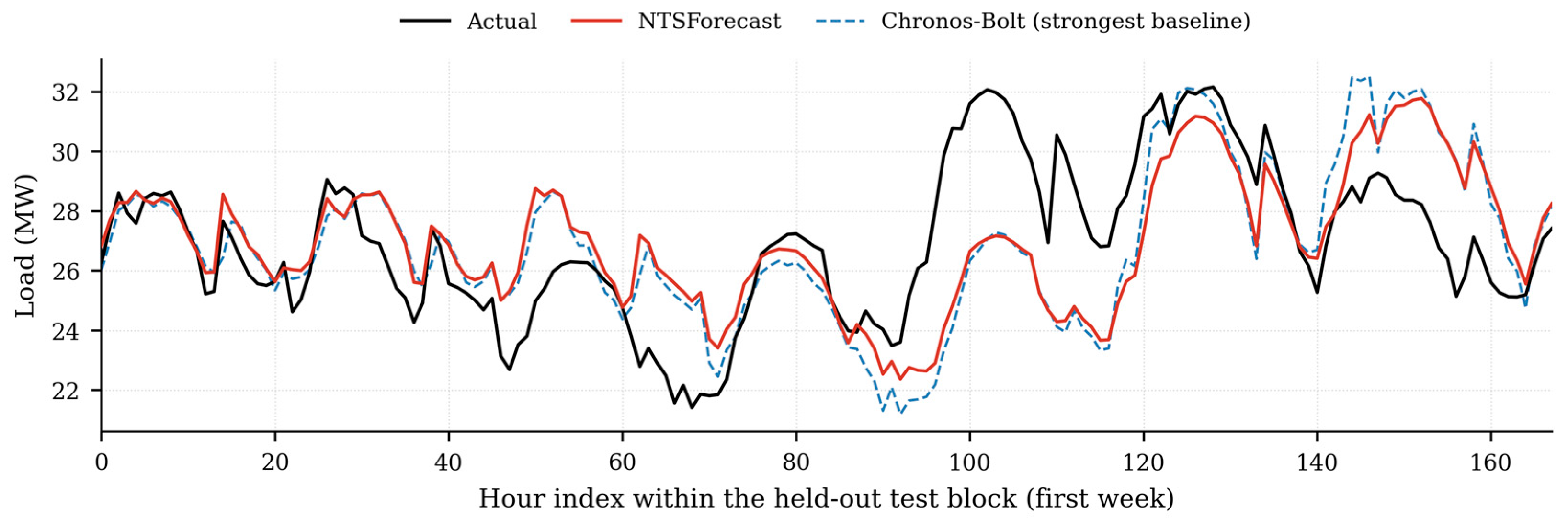
Figure 6 places the actual load curve, the NTSForecast forecast and the forecast of the strongest baseline of Table 3 on the same time axis for the first week (168 h) of the held-out evaluation period. The framework’s curve is the average of the five seed runs, plotted for readability only; every quantitative comparison in this paper is computed per seed. The visual impression matches Table 3: the daily cycle dominates, both forecasts track it closely, and the differences that separate the methods statistically are small at the scale of the plot, which is why the comparison is settled by the significance test rather than by inspection.

6.4. Error Distribution Analysis

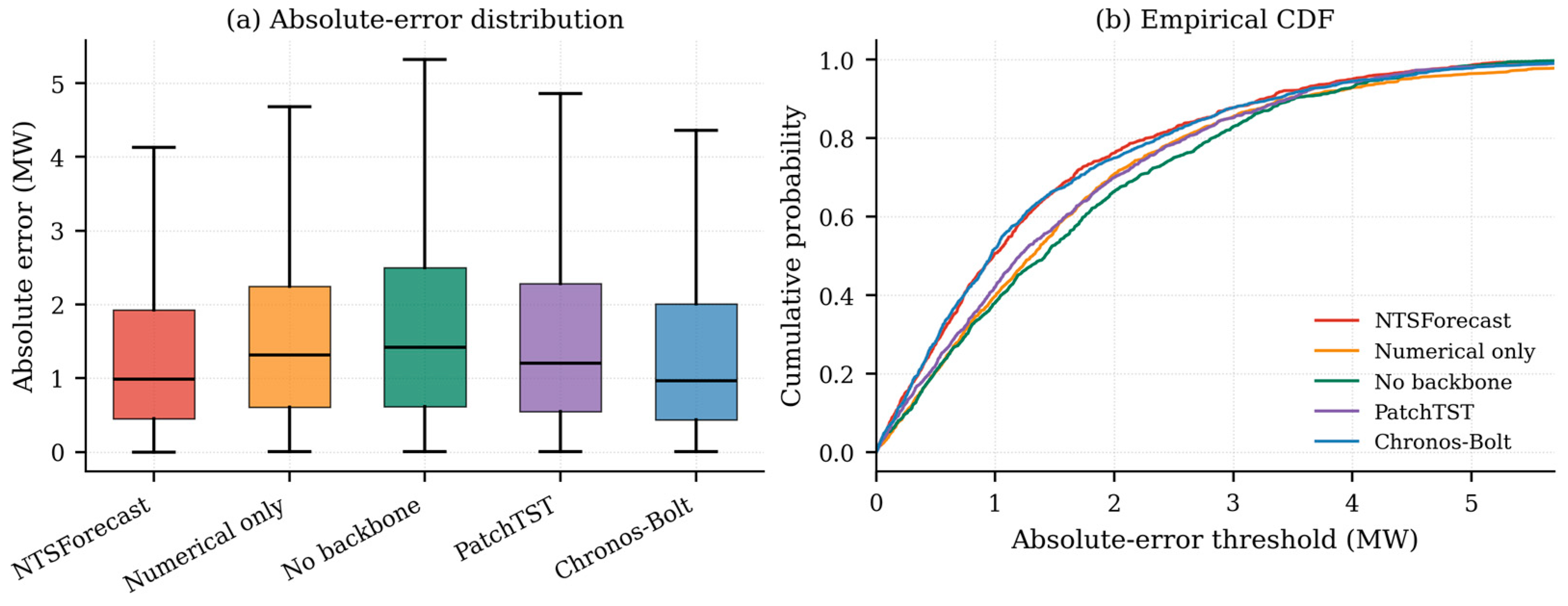
To compare forecast quality beyond aggregate metrics, Figure 7 shows the absolute-error distribution of NTSForecast on the held-out test set (7824 samples) from two perspectives. (a) The boxplot gives the median, interquartile range and extreme values of the absolute errors; the median reflects overall accuracy, and the interquartile range reflects consistency. (b) The empirical cumulative distribution function shows the proportion of forecasts falling below a given absolute-error threshold, which is the quantity of operational interest when a tolerance band is specified.

6.5. Training Dynamics

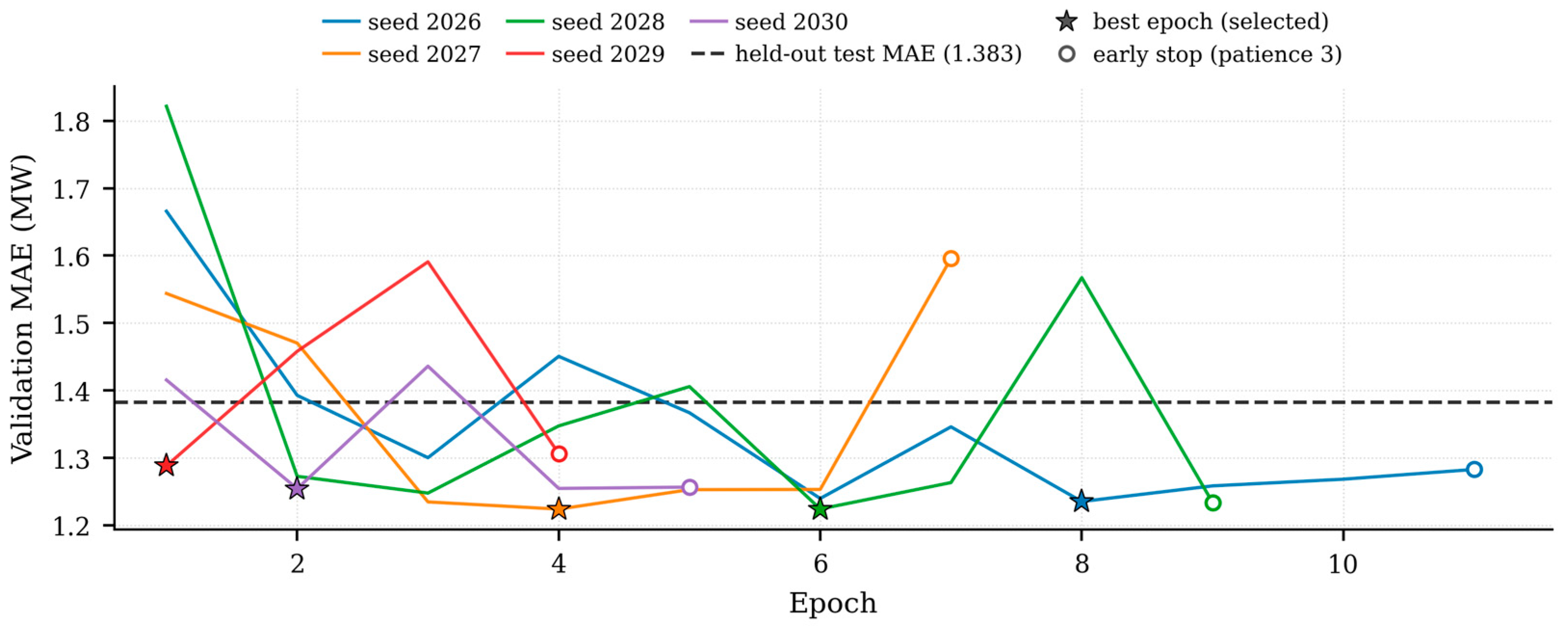
Figure 8 shows the convergence behaviour of NTSForecast. (a) The training loss decreases monotonically, and its slope flattens once the trainable modules have largely converged. (b) The validation error is used for epoch selection and for early stopping; the held-out test error is computed once, after training is complete, and is materially higher than the validation error. We report both because the size of that gap is what determines whether a validation-selected model transfers to an unseen period, and it is not visible when a single split serves both purposes.

6.6. Channel Ablation, Backbone-Scale Study and Subgroup Analysis

Two ablations are run under the protocol of Section 6.1, with the configuration, data and seeds of the full model held fixed: one removes the text channel, the other the numerical channel. Removing the text channel raises MAPE from 5.6621 ± 0.0448 to 6.8280 ± 0.5833, a loss of 1.17 percentage points that exceeds the seed spread of either variant. Removing the numerical channel gives 6.1083 ± 0.2942, which is not the contribution of that channel: without it the model has no sample-varying input, its predictions on the held-out blocks have zero dispersion, and the error is that of a constant forecast. This run serves only as a sanity check.

Two further controls isolate what the text channel supplies. Scrambling the word order of the task description, at equal token length and with the same vocabulary, gives MAPE 5.6582 ± 0.0390; replacing the description with a learnable prefix of equal length gives 5.7029 ± 0.0327; the full model gives 5.6621 ± 0.0448. Neither control moves the mean beyond the seed-to-seed spread.

The channel therefore carries weight, but not through its linguistic content. This is what the corpus predicts: the task description and the field labels are identical in every sample, so there is no sample-level semantic content to convey, and the channel acts as a stable, high-dimensional conditioning signal on which the numerical encoder is aligned. Operational text that does vary with the sample, such as maintenance and switching orders, outage notices, holiday and production schedules or severe-weather warnings, can travel the same pathway. Demonstrating that requires a corpus in which such records are time-aligned with the load series, which this dataset does not provide. Ablating the text channel degrades accuracy most where forecasting is hardest—the largest significant MAPE increases (bootstrap 95% CIs excluding zero) occur on the bottom load decile (−3.51 pp); the holiday weeks (Thanksgiving and the December break) (−1.80 pp); the extreme pressure deciles (−1.64 pp); the quartile with the largest 24 h temperature swing (−1.63 pp)—indicating that the constant text embedding stabilizes the learned representation precisely on the samples least served by historical extrapolation. The reversal is reported with equal prominence: on the top load decile (+0.79 pp) the text-ablated variant is significantly more accurate, so the effect is a trade-off across operating conditions rather than a uniform gain. All subgroup comparisons are tested with bootstrap confidence intervals, and the subgroups on which the comparison favours the ablated variant are reported above alongside those on which it does not.

Table 4. Channel ablations and two equal-length text controls: a word-order-scrambled task description with the same tokens, and a learnable constant prefix of the same length. All variants use the configuration, data and seeds of the full model; values are mean ± standard deviation over five seeds. * This variant has no sample-varying input and is retained only as a sanity check.

Model Variant	MAE	RMSE	MAPE/%
Numerical channel only (text ablated)	1.8248 ± 0.1612	2.4701 ± 0.2115	6.8280 ± 0.5833
Text channel only (numerical ablated) *	1.6183 ± 0.0775	2.2403 ± 0.0867	6.1083 ± 0.2942
Word-order-scrambled task description (equal length)	1.4942 ± 0.0123	2.0745 ± 0.0164	5.6582 ± 0.0390
Learnable constant prefix (equal length)	1.5048 ± 0.0078	2.0949 ± 0.0081	5.7029 ± 0.0327
Full NTSForecast	1.4926 ± 0.0113	2.0672 ± 0.0071	5.6621 ± 0.0448

collects these results.

The same protocol supports a backbone-scale study, in which the frozen backbone is replaced while architecture, data and seeds are held fixed, and the projection widths follow the hidden size of the backbone in use; a randomly initialized backbone of the largest size attains MAPE 5.8742 ± 0.1448, Qwen2.5-0.5B 5.6621 ± 0.0448, Qwen2.5-1.5B 5.6889 ± 0.0254 and Llama-3.1-8B 5.9714 ± 0.2120. This ordering is the opposite of what a capacity argument predicts. The smallest pretrained backbone is the most accurate of the four, accuracy does not improve monotonically with size, and the largest pretrained backbone is the least accurate, indistinguishable from the randomly initialized control of the same size.

The explanation is a sample-size effect. The binding constraint at 94 training samples is the pair of alignment projections between the numerical channel and the backbone, whose width follows the hidden size of the backbone. A larger backbone widens them, and a seven-day record cannot supply enough supervision to fit the wider mapping, so whatever semantic prior a larger model holds stays out of reach. The seed-to-seed spread follows the same pattern, growing from 0.0448 at 0.5B to 0.2120 percentage points at 8B. Qwen2.5-0.5B is therefore adopted as the reference configuration: most accurate on this task, smallest seed-to-seed spread, and cheapest in memory and latency, as Section 7.1 quantifies.

The ladder deliberately omits one substitution. The domain-specific time-series foundation models of Table 3 cannot serve as the backbone: they accept numerical series only, and with neither a tokenizer nor a text-embedding layer they cannot instantiate the textual channel on which a numerical–textual framework rests. Replacing the backbone with one of them would give a different, numerical-only model rather than a variant of NTSForecast, so they are evaluated as the zero-shot forecasters they were built to be and appear in Table 3 among the baselines.

6.7. Bayesian Optimization on the Full Model

This subsection reports the Bayesian optimization of the full model: the LLM backbone remains frozen, and the search covers the five hyperparameters of Table 2. The budget is 24 TPE trials of six epochs each, scored exclusively on the validation window; the held-out test set plays no role in the search. Consistent with the relabelling of this section as a sensitivity study, the outputs we report are the search trajectory and the stability of the importance estimates, not a ranking.

Figure 9a shows the search trajectory of the 24 trials, scored on the validation subset only, so that the held-out blocks take no part in model selection. The most informative feature of the trajectory is how little it moves: the running best improves from 5.248 to 5.235 percent, a total of 0.013 percentage points over the whole budget, and 21 of the 24 trials fall within a band of 0.5 percentage points. We read this as a property of the model rather than a failure of the search. Accuracy here is not contingent on locating a particular corner of the hyperparameter space: learning rate, weight decay, batch size, accumulation depth and activation can all be varied over the ranges of Table 2 without materially changing the outcome. For a method intended for feeders that are commissioned with a week of history and no tuning budget, that insensitivity is the operationally relevant property, and it is worth more than the 0.013 percentage points the search itself returns. The search retains a second use, which is the importance analysis reported below: even when the achievable gain is small, the sampled trials support a relative ranking of the hyperparameters and thereby indicate where a practitioner should look first. What the budget does not support is a claim of global near-optimality, and we do not make one. Procedurally, the located configuration is the one stated in Section 6.1 and used unchanged for the full model and every variant reported, so the search and the results are consistent by construction.

Table 5. Best hyperparameter configuration located by the Bayesian optimization study on the validation split. It is used unchanged for the full model and for every variant reported in this manuscript.

Hyperparameter	Best Value
learning rate	3.35 × 10−3
weight decay	2.05 × 10−5
batch size	2
accum steps	1
activation	ReLU
validation MAPE	5.23%

lists the configuration located by the search.

6.8. Per-Origin Breakdown Across the Six Rolling Origins

Table 3 pools the six origins into a single year-long series before computing metrics, which is the correct way to obtain seed-level dispersion but hides how much the individual origins differ. This subsection reports that breakdown. The protocol of Section 6.1 is held fixed, and the origin is the only thing that moves: at each origin the seven-day raw record immediately preceding the validation window supplies the 94 training samples, the following 1302 h form the validation window and the next 1304 h the test window, and the six test windows are consecutive and non-overlapping, so their union is the 9 February 2019 to 31 December 2019 evaluation period of 7824 hourly points used in Table 3. Every method is retrained from scratch at every origin; nothing is carried across origins except the code. A single hyperparameter configuration, located once by the Bayesian optimization of Section 4, is applied unchanged at every origin, and no per-origin tuning is performed for any method. The origins differ in difficulty before any model is trained, and the difficulty is measurable in advance: the mean load of the seven-day training record differs from that of the corresponding test window by −6.7% at the most favourable origin and by +35.5% at the least favourable one, so the six origins span the range from a well-matched window to a window that misrepresents the deployment period by more than a third.

Table 6. Per-origin results under the main setting. The second column is the hold-out test window, the period over which that row’s errors are computed; it is not an input window. The third column is the 168 h record on which the trainable parameters are fitted, and validation lies between the two. Entries are MAPE (%) averaged over five random seeds; the final row is the mean ± standard deviation across origins. One hyperparameter configuration is used at every origin, with no per-origin tuning for any method.

Origin	Hold-Out Test Window	Training Record (168 h)	NTSForecast	Chronos-Bolt (Zero-Shot)	Time-LLM	Parameter-Matched MLP
Origin 1	9 February 2019 to 4 April 2019	9 December 2018 to 16 December 2018	5.46	5.44	5.57	7.09
Origin 2	4 April 2019 to 28 May 2019	2 February 2019 to 9 February 2019	5.40	5.45	5.71	7.20
Origin 3	28 May 2019 to 21 July 2019	28 March 2019 to 4 April 2019	5.63	5.79	6.01	6.74
Origin 4	22 July 2019 to 14 September 2019	21 May 2019 to 28 May 2019	5.66	5.66	5.75	6.81
Origin 5	14 September 2019 to 7 November 2019	15 July 2019 to 22 July 2019	6.23	6.05	6.39	7.04
Origin 6	7 November 2019 to 31 December 2019	7 September 2019 to 14 September 2019	5.59	5.67	5.66	7.35
Mean across origins	—	—	5.66 ± 0.27	5.68 ± 0.21	5.85 ± 0.28	7.04 ± 0.21

gives the per-origin figures. Against the strongest baseline of Table 3 the framework attains the lowest MAPE at four of the six origins, and its across-origin mean of 5.66 ± 0.27 is below that baseline’s 5.68 ± 0.21. At the two remaining origins the two methods lie within 0.18 percentage points of each other, and at Origin 4 they agree to two decimal places. Those origins are listed individually instead of being absorbed into the mean. Against the parameter-matched MLP the ordering is uniform: the complete structure is more accurate at every origin, by between 0.81 and 1.80 percentage points, which is the per-origin form of the controlled comparison in Section 6.6. The spread across origins carries its own information. The framework’s per-origin MAPE varies by 0.83 percentage points over the six windows, and that variation belongs to the window, not to the method. The per-origin figures of the framework and of the strongest baseline move together almost perfectly (Pearson r = 0.94 across the six origins), so an origin that is hard for one is hard for the other. The level gap of the preceding paragraph does not predict which origins those are: the origin with the largest gap (+35.5%) is one of the framework’s better windows. Window representativeness is thus more than a difference in mean level, and Section 7.4 carries the residual dependence on it as a limitation.

7. Discussion

7.1. Operating Envelope: What the Frozen Backbone Contributes, Where It Stops, and What It Costs

This section asks three things of the frozen backbone: whether it contributes at all, where its contribution stops, and what it costs. The first is settled by the parameter-matched comparison, in which a numerical encoder keeps the architecture, the trainable-parameter count (1,841,793), the hyperparameters and the data of the full model and loses only the backbone: on the HEEW dataset removing the frozen backbone raises MAPE by 1.38 percentage points (7.0374 without it versus 5.6621 with it; Welch t-test on per-seed MAPE, p = 0.0038). Two further comparisons run the same way. A randomly initialized backbone reaches 5.8742 ± 0.1448 against 5.6621 ± 0.0448, which separates pretraining from architecture, and LoRA adaptation of the same backbone reaches 10.8546, so under a window this short adapting the backbone is worse than leaving it alone.

Where the contribution stops depends on what a method has to estimate. Every baseline that must learn the load–weather mapping from the seven-day record without a large pretrained prior falls well behind: the parameter-matched encoder, the randomly initialized backbone, LoRA adaptation, the classical regressors, the compact linear-decomposition and patch-based forecasters, and the recurrent and attention sequence models. Only the methods that bring such a prior stay close, namely Time-LLM (5.8491) and the three zero-shot foundation models (5.6772, 5.7749 and 5.9186), and the framework leads them by a fraction of a percentage point rather than by the margin that separates the bands. What matters is the presence of a pretrained prior, not its size, since the ladder is non-monotonic, and the largest backbone is the least accurate. The error common to the whole leading band is then not a limit on capacity but the distribution gap between a seven-day training record and a deployment period up to a third away from it in level, which Section 6.8 quantifies origin by origin. This is what the architecture buys in the scarce-history regime: 94 training samples reach the accuracy that purpose-built pretraining at nine orders of magnitude larger scale delivers on the same task.

The cost is measured rather than argued. In the reference configuration NTSForecast needs 1445 MB of peak GPU memory and 28.59 ms per forecast, against 995 MB and 7.17 ms for GPT4TS. Because the reference backbone is the smallest rung of the ladder, that is an order of magnitude below the same design at 8B (17,164 MB, 51.17 ms), which Section 6.6 also shows to be the less accurate of the two. Training is far cheaper than full fine-tuning or LoRA adaptation of the same backbone because no backbone parameter is updated, and no optimizer state is held for it. The efficiency claim is scoped accordingly: it holds against adaptation of the same backbone, not as a general claim about deployability.

The framework never fine-tunes the backbone. The pretrained decoder serves only as a context-processing component in the forward pass, and its weights stay frozen in training and in inference alike. Against LoRA or full-parameter fine-tuning this removes the optimizer state and the gradient computation for the backbone, which is where the training-cost advantage comes from. The advantage stops at training. Both settings run the full backbone in the forward pass, so freezing buys nothing in latency or peak memory, and the figures above leave both an order of magnitude above a compact baseline. Any statement about deployability has to keep that distinction.

Table 7. Computational cost under the protocol of Section 6.1, measured on the hardware and software stack of Section 5. NTSForecast with the frozen Qwen2.5-0.5B backbone is the reference configuration; the Llama-3.1-8B row is the largest rung of the ladder of Section 6.6, and LoRA represents backbone adaptation.

Configuration	Trainable Params	Peak GPU Memory (MB)	Wall-Clock per Epoch (s)	Inference Latency (ms/Forecast)
Parameter-matched MLP	1,841,793	59	0.2	0.49
GPT4TS	814,849	995	0.3	7.17
LoRA adaptation of the same backbone	2,382,465	1791	3.0	139.34
NTSForecast (frozen Qwen2.5-0.5B)	1,841,793	1445	1.1	28.59
NTSForecast (frozen Llama-3.1-8B)	8,404,993	17,164	2.5	51.17
Time-LLM	143,958,913	39,428	935.1	138.11

reports the measurements for every configuration.

7.2. Relation to Compact Multimodal Forecasters

A compact, non-LLM demonstration of the same premise helps place the present contribution. The convolutional-recurrent ensemble of [17] integrates multimodal inputs for day-ahead electricity-price forecasting without serializing anything into a language model, and it reports gains from that integration. Two things follow. Multimodal fusion by itself is not what a frozen language backbone provides, since a compact supervised architecture can fuse heterogeneous inputs and profit from it. The claim made here is the narrower one, about what the frozen backbone adds on top of fusion, which is why the controlled comparison of Section 6.6 fixes the fusion architecture and the trainable-parameter count and varies only the presence of the backbone. That line of work also supplies the cost reference against which a language backbone has to be judged, and the same comparison runs inside our own experiments: the parameter-matched encoder trains the same 1,841,793 parameters as the full framework, peaks at 59 MB and forecasts in 0.49 ms, against 1445 MB and 28.59 ms for the proposed framework, at a MAPE difference of 1.38 percentage points in the framework’s favour. Whether that accuracy is worth that overhead is an application-level decision, and both sides of it are on the table here.

7.3. Hyperparameter Sensitivity: What the Importance Analysis Does and Does Not Establish

The hyperparameter importance analysis serves as a reference, not as a result. Bootstrapping the fANOVA estimates over the 24 trials yields 95% confidence intervals whose mean width is 45.3 percentage points, and the interval for the learning rate alone runs from 12 to 86 percent of the explained variance. No numerical ranking survives that. A second observation points the same way, and it bears on how such analyses should be read in general. We ran the identical search space and trial budget twice, changing only the frozen backbone. The leading term held, with the activation function first in both runs, but the rest of the order was rearranged: accumulation depth fell from second to fourth while the learning rate rose, and the two located learning rates differed by more than two orders of magnitude. Hyperparameter importance is thus conditional on the input window, the backbone and the search space. It is not a transferable property of the method. The analysis is useful for direction, not magnitude. It shows where a practitioner adapting the framework to another feeder should look first, and we report it with that scope. It should be read together with Section 6.7, where the same trials show that accuracy varies little across the searched ranges. A nearly flat response surface makes the decomposition of a small variance unstable, and the flatness is the more useful finding of the two.

7.4. Limitations and Outlook

Four limitations bound the envelope of Section 7.1. First, the forward pass executes the full backbone whether or not it is frozen. Taking the smallest rung of the ladder as the reference configuration cuts that cost by an order of magnitude relative to 8B, and Section 7.1 reports both, but a compact supervised model is cheaper still wherever latency or memory is tightly constrained. Second, the margin is small exactly where the comparison is closest. Against the methods that also bring a large pretrained prior, Time-LLM and the three zero-shot foundation models, the advantage is a fraction of a percentage point of MAPE. It is significant under the per-seed test on the pooled evaluation period, and Section 6.8 gives the individual origins where it does not hold.

Third, the envelope rests on one region and one deployment period. The boundary reported here, that a frozen backbone recovers much but not all of the deficit from learning on a short window and that backbone scale does not move that boundary, is supported by a single dataset. The rolling-origin protocol of Section 6.8 tests it across four seasons of one deployment period; testing it fully would take the same protocol on further datasets, regions and load profiles, which is the natural continuation of this study. Fourth, the design targets the seasonal drift between training and deployment periods, a form of dataset shift [37]. Demand itself is changing as flexible resources are adopted, so the weather–load mapping is a moving target, and the robustness effect of Section 6.6 deserves re-examination over horizons longer than we can cover here.

8. Conclusions

This paper presents NTSForecast, a numerical–textual dual-channel framework for short-term load forecasting that combines a trainable numerical encoder with a strictly frozen pretrained LLM, leaving every backbone parameter untouched. The evaluation stays inside the regime the method is built for. At each of six rolling origins the only history available for training is a seven-day raw record, which yields 94 training samples, and the six non-overlapping test windows together cover 7824 held-out hourly points. Five seeds and Diebold–Mariano testing support four conclusions. First, on accuracy: The framework attains the lowest MAE, RMSE and MAPE of every method compared. The margin over the strongest baseline, Chronos-Bolt-Base applied zero-shot, is 0.02 percentage points of MAPE and holds under the shorter of the two bandwidths examined in Section 6.2, so the framework is competitive with that baseline rather than superior to it. Second, on the source of that accuracy: On the HEEW dataset removing the frozen backbone raises MAPE by 1.38 percentage points (7.0374 without it versus 5.6621 with it; Welch t-test on per-seed MAPE, p = 0.0038). Since the two variants share architecture, trainable-parameter count, hyperparameters and data, that difference belongs to the frozen backbone and not to capacity or tuning. The same direction holds against a randomly initialized backbone of the same size and against LoRA adaptation, which on a seven-day record is markedly worse than leaving the backbone frozen. Third, on backbone scale: Accuracy across the random-initialization/0.5B/1.5B/8B ladder is non-monotonic and runs against a capacity argument, the smallest pretrained backbone being the most accurate and the largest the least. A sub-billion-parameter backbone is therefore adopted as the reference configuration, and the remaining error is attributed to the distribution gap between the seven-day training record and the deployment period. The ladder spans four backbones on one dataset, enough to rule out a monotone capacity effect here but not to establish a general scaling law. Fourth, on the text channel: Ablating it costs 1.17 percentage points, yet destroying the semantic content while keeping the channel in place changes accuracy by less than 0.01 percentage points. The textual side of this dataset is a fixed instruction and a set of field labels rather than sample-level operating information, so semantic content is not what the channel contributes.

Two boundaries come with these results: the margin over the methods that also carry a large pretrained prior is a fraction of a percentage point and does not hold at every origin, and the hyperparameter-importance analysis is a sensitivity study rather than a ranking because the trial budget cannot support stable importance estimates. Future work should establish whether a sample-varying text channel turns the conditional effect seen here into a consistent gain, whether the envelope reproduces on other regions and load profiles, and whether distillation can remove the remaining backbone cost.