A Graph–Physics-Constrained Fast State Estimation Method for Wind/PV Integrated Transmission Networks

Abstract

The increasing penetration of wind and photovoltaic (PV) generation introduces frequent operating-point variations into transmission networks, while missing supervisory control and data acquisition/phasor measurement unit (SCADA/PMU) measurements and bad data may further weaken the reliability of online state estimation. Conventional weighted least squares (WLS) estimators have a clear physical interpretation, but repeated online matrix solutions may become burdensome in large-scale rolling estimation. To address this issue, this paper proposes a graph–physics-constrained fast state estimation method with bad data detection (BDD) and filtering. Wind/PV-load operating scenarios are constructed on standard test systems, and mixed SCADA/PMU measurements are represented with missing masks and bad data perturbations. The filled measurements, measurement availability mask, and residual anomaly scores are used as input features, while the network topology is converted into a graph Laplacian prior. A regularized fast mapping, graph Laplacian smoothing, and threshold-calibrated residual screening are combined to obtain online state estimates and bad data labels. Five-seed case studies compare the proposed method with WLS and Huber robust WLS. In case300, the average online time is reduced from $66.063\pm 3.054$ ms for WLS to $1.922\pm 0.374$ ms for the proposed method, corresponding to a speedup of about 35.08 times. The results indicate that the proposed linearized prototype is most promising as a fast large-scale rolling estimator or abnormality screener, rather than as a full replacement for model-based estimators in all scenarios.

1. Introduction

Power system state estimation is a fundamental function of energy management systems (EMSs) and dispatch automation systems. Its core task is to estimate bus voltage magnitudes and phase angles under measurement noise, measurement redundancy, and network-topology constraints. The static state estimation model was systematically formulated in reference [1], where redundant measurements are converted into estimates of the system state vector, laying the theoretical basis for weighted least squares (WLS) state estimation. The role of state estimation in EMS real-time network modeling was summarized in reference [2], which emphasized that state estimation constructs a quasi-static network model from real-time measurement snapshots. Observability analysis, bad data detection, parameter estimation, and topology-error processing were further reviewed in reference [3]. Therefore, conventional WLS methods are attractive because of their physical interpretability, clear statistical meaning, and engineering maturity. However, their online execution usually requires repeated construction and solution of normal equations, and the computational burden increases under large-scale and high-frequency rolling estimation.

With the development of phasor measurement units (PMUs), wide-area measurement systems (WAMSs), advanced metering infrastructure (AMI), and intelligent terminals, state estimation has evolved from single-source supervisory control and data acquisition (SCADA) measurements to multi-source heterogeneous measurement fusion. A recent survey on multi-source state estimation using PMUs, SCADA, AMI, and other data sources [4] pointed out that data integration must handle differences in sampling rate, synchronization accuracy, measurement type, and data quality. A synchrophasor-based real-time state estimation system was discussed in reference [5], showing that PMUs can improve dynamic awareness, while measurement latency, packet loss, and local unobservability still affect reliability. The use of PMU measurements to supplement SCADA measurements was studied in reference [6], which is meaningful for transmission networks with insufficient PMU coverage. These studies indicate that hybrid SCADA/PMU measurements can improve observability and dynamic response, but they also make missing measurements, asynchronous sampling, and abnormal-data processing more complicated.

Large-scale renewable integration further changes the operating background of state estimation. Wind and PV outputs are stochastic, intermittent, and strongly correlated with weather conditions, which makes the operating point of transmission networks vary more frequently. A renewable-energy management system implementation based on a fast decoupled WLS framework was proposed in reference [7] to handle renewable modeling, topology errors, and measurement errors. Reviews on distribution system state estimation with renewable energy sources further indicate that renewable integration increases the difficulty of monitoring and power-quality assurance, requiring state estimation methods to adapt to high uncertainty and diverse measurement conditions [8]. Non-deterministic state estimation studies also suggest that real-time monitoring algorithms should explicitly consider randomness and correlation when measurement errors, communication anomalies, and renewable pseudo-measurement uncertainty increase [9].

Bad data detection and robust state estimation form an important branch of conventional state estimation research. Least median of squares was introduced into power system state estimation in reference [10] to improve robustness under abnormal measurements. The least absolute value (LAV) robust state estimation for PMU-measured systems was studied in reference [11], showing that absolute-value-based objectives can reduce the influence of outliers. From a cyber-security perspective, false-data injection attacks were modeled in reference [12], proving that attackers can construct attack vectors that bypass conventional bad data detectors. Malicious data attacks on smart grids were further discussed in reference [13], and the vulnerability of alternating-current (AC) state estimation to false-data injection was analyzed in reference [14]. A survey of false-data injection attacks, impacts, and defenses [15] emphasized that residual-based bad data detection (BDD) is limited under coordinated and structured anomalies.

In recent years, machine learning, graph learning, and physics-constrained learning have provided new paths for fast state estimation. Graph convolution can propagate features through node connections [16], and surveys on graph neural networks (GNNs) indicate that graph priors are suitable for non-Euclidean network data [17]. Physics-informed neural networks (PINNs) and physics-informed machine learning introduce physical equations, conservation constraints, or structural priors into learning processes, thereby reducing dependence on sample size and improving extrapolation behavior [18,19]. Physics-informed geometric deep learning was applied to state estimation and power-flow inference tasks in reference [20]. Physics-informed graphical neural networks further combine graph learning with model-based estimation for state estimation under limited measurements [21]. Recent work on spatio-temporal dynamic GNNs for missing-measurement recovery directly targets random and continuous missing scenarios, showing that missing masks and spatio-temporal correlation are important for learning-based state estimation [22]. Neural-network state estimation and deep statistical solvers also show that learning models can reduce online computation time after offline training, but their observability, extrapolation stability, and physical consistency still require network models and constraints [23,24].

In summary, four research gaps remain. First, conventional WLS, LAV, and robust estimation studies emphasize accuracy and robustness, but they seldom take online computation time in large benchmark systems as a primary comparison metric. Second, state estimation studies under wind/PV uncertainty often focus on uncertainty modeling or filtering, while a unified framework for missing measurements, bad data filtering, and fast online estimation is still insufficient. Third, although learning-based state estimation has adopted GNNs, PINNs, and physics-constrained models, some studies rely on complex neural network training, and the connection with conventional state-estimation workflows requires further strengthening. Fourth, bad data research has developed from residual detection to false-data injection defense, but more evidence is needed for fast state estimation prototypes that simultaneously report estimation errors, detection F1-score, and online time.

Compared with general graph signal processing methods, the novelty of this work is not only the use of a graph Laplacian but also its integration into a complete state-estimation workflow that jointly handles hybrid SCADA/PMU measurements, missing masks, residual anomaly scores, fast online mapping, and threshold-calibrated bad data filtering. The proposed method should therefore be understood as a graph topology-assisted fast estimator for a linearized state-estimation prototype, rather than as a general-purpose graph signal denoising method.

To balance computational speed, abnormal-measurement processing, and engineering interpretability, this paper adopts a graph–physics-constrained fast estimation route. The key idea is to construct a graph Laplacian prior from network topology, combine hybrid measurements, missing masks, and anomaly residual scores as input features, learn the state-estimation mapping through a fast estimator, and perform residual detection and bad data filtering online.

The main contributions are as follows:

(1)

A simulation framework for wind/PV-integrated transmission networks is constructed, incorporating renewable stochastic output, hybrid SCADA/PMU measurements, missing-measurement masks, and bad data disturbances into a unified testing process.

(2)

A fast estimation model combining graph topology priors, regularized fast mapping, Laplacian smoothing, and residual-based bad data filtering is proposed, preserving an explicit link with grid topology while keeping online computation lightweight.

(3)

Comparative experiments are conducted on case39, case118, and case300 standard systems. Estimation errors, bad data detection performance, and online computation time are reported to evaluate the proposed method against WLS and Huber robust WLS.

The rest of this paper is organized as follows: Section 2 establishes the measurement, missing-data, bad data, and graph topology models. Section 3 presents the proposed fast state estimation method and algorithmic procedure. Section 4 reports case studies and experimental analysis. Section 5 concludes the paper.

2. System Modeling and Problem Description

2.1. State Estimation Measurement Model

To remain consistent with the standard systems used in the case studies, this paper first constructs a linearized hybrid-measurement state estimation model. Suppose that the transmission network contains N buses, with bus 1 selected as the reference bus. The state vector consists of the phase angles of non-reference buses and the voltage magnitude deviations of all buses:

$$\mathit{x}={\left[{\theta }_2,{\theta }_3,\dots ,{\theta }_N,\Delta V_1,\Delta V_2,\dots ,\Delta V_N\right]}^T.$$

(1)

Here, $\mathit{x}\in {\mathbb{R}}^{2N-1}$ is the system state vector, N is the number of buses, ${\theta }_i$ is the voltage phase angle of bus i, and $\Delta V_i$ is the voltage magnitude deviation of bus i from the nominal operating value. Bus 1 is used as the phase-angle reference, so ${\theta }_1$ is not included in $\mathit{x}$.

The hybrid measurement vector includes bus active power injections, branch active power flows, voltage magnitudes, and partial PMU phase-angle measurements. In the linearized prototype, the measurement model is written as

$$\mathit{z}=\mathit{H}\mathit{x}+\mathit{e},$$

(2)

where $\mathit{z}\in {\mathbb{R}}^M$ is the hybrid measurement vector, M is the number of measurements, $\mathit{H}\in {\mathbb{R}}^{M\times (2N-1)}$ is the measurement matrix constructed from branch topology and branch reactance, and $\mathit{e}\in {\mathbb{R}}^M$ denotes zero-mean measurement noise. The conventional WLS estimation objective is

$$\underset{\mathit{x}}{min}J\left(\mathit{x}\right)={\left(\mathit{z}-\mathit{H}\mathit{x}\right)}^T{\mathit{R}}^{-1}\left(\mathit{z}-\mathit{H}\mathit{x}\right).$$

(3)

In this objective, $J\left(\mathit{x}\right)$ is the weighted residual cost and $\mathit{R}\in {\mathbb{R}}^{M\times M}$ is the measurement-noise covariance or weighting matrix.

To avoid ill-conditioning caused by missing measurements and bad data, the WLS benchmark uses a small regularization term:

$${\mathit{x}}_{\mathrm{WLS}}={\left({\mathit{H}}_a^T{\mathit{R}}_a^{-1}{\mathit{H}}_a+{\lambda }_{\mathrm{WLS}}\mathit{I}\right)}^{-1}{\mathit{H}}_a^T{\mathit{R}}_a^{-1}{\mathit{z}}_a.$$

(4)

Here, ${\mathit{x}}_{\mathrm{WLS}}$ is the regularized WLS estimate, a denotes the active observed-measurement index set after excluding missing measurements and previously screened bad data candidates, and ${\mathit{H}}_a$, ${\mathit{R}}_a$, and ${\mathit{z}}_a$ are the corresponding active rows/submatrices of $\mathit{H}$, $\mathit{R}$, and $\mathit{z}$, respectively. The identity matrix $\mathit{I}$ has dimension $(2N-1)\times (2N-1)$, and ${\lambda }_{\mathrm{WLS}}$ is used only for numerical regularization of the WLS benchmark.

The actual AC state-estimation problem is nonlinear. The present work intentionally uses a linearized prototype to evaluate whether topology-assisted fast mapping and residual filtering can reduce online computation under renewable scenario variations. Therefore, the proposed method is not claimed as a complete replacement for full AC state estimation; rather, it is positioned as a fast-rolling estimator or abnormality screener that can be further extended to nonlinear AC models.

2.2. Missing-Measurement and Bad Data Model

In practical dispatch systems, SCADA/PMU measurements may be missing because of communication interruption, device abnormality, or synchronization failure. To avoid treating missing values as true zeros, this paper uses a binary mask $\mathit{m}$ to describe measurement availability:

$$m_i=\left\{\begin{array}{cc}1,\hfill & \mathrm{measurement}\mathrm{available},\hfill \\ 0,\hfill & \mathrm{measurement}\mathrm{missing}.\hfill \end{array}\right.$$

(5)

Here, $\mathit{m}={[m_1,\dots ,m_M]}^T$ is the measurement-availability mask, $m_i$ is the binary availability indicator of the ith measurement, and M is the total number of measurements.

The measurement model with bad data is

$${\mathit{z}}_b=\mathit{H}\mathit{x}+\mathit{e}+\mathit{a},$$

(6)

where ${\mathit{z}}_b\in {\mathbb{R}}^M$ is the contaminated measurement vector and $\mathit{a}\in {\mathbb{R}}^M$ is the bad data disturbance vector. If the ith measurement is not contaminated, then $a_i=0$; otherwise $a_i\ne 0$. In the baseline setting, the missing-measurement rate is 10%, and the bad data ratio is 5%. For each observed measurement, bad data positions are sampled independently according to the specified ratio. The nonzero disturbance amplitude is sampled as $|a_i|=(6+6u_i){\sigma }_i$, where $u_i$ is a scalar random variable following $U(0,1)$ and ${\sigma }_i$ is the standard deviation of the ith measurement noise. Its sign is sampled from a symmetric Bernoulli distribution. Thus, the disturbance magnitude ranges from $6{\sigma }_i$ to $12{\sigma }_i$.

2.3. Graph Topology Prior

Grid topology is one of the most stable and interpretable sources of prior information for state estimation. A weighted graph $G=(V,E)$ can be constructed from branch data, where nodes represent buses and edges represent transmission lines or transformer branches. Let the branch reactance be $x_{ij}$; the branch weight is approximated as $b_{ij}=1/max\left(\right|x_{ij}|,{10}^{-4})$ in the simulations so that all Laplacian weights remain nonnegative. The graph Laplacian is defined as

$$\mathit{L}=\mathit{D}-\mathit{A},$$

(7)

where $\mathit{A}\in {\mathbb{R}}^{N\times N}$ is the weighted adjacency matrix, $\mathit{D}\in {\mathbb{R}}^{N\times N}$ is the weighted degree matrix, and $\mathit{L}\in {\mathbb{R}}^{N\times N}$ is the graph Laplacian. Since voltage angles and magnitude deviations of electrically adjacent buses are usually continuous to some extent, the following graph-smoothing term can suppress nonphysical jumps between neighboring buses:

$$\mathrm{\Omega }\left(\mathit{x}\right)={\mathit{x}}^T{\mathit{L}}_s\mathit{x}.$$

(8)

Here, $\mathrm{\Omega }\left(\mathit{x}\right)$ is the graph-smoothing penalty and ${\mathit{L}}_s$ is the state-space Laplacian aligned with the dimension of $\mathit{x}$. Because the state vector contains $N-1$ non-reference phase angles and N voltage magnitude deviations, the state-space Laplacian is constructed as

$${\mathit{L}}_s=\mathrm{blkdiag}\left({\mathit{L}}_{\theta },{\mathit{L}}_V\right),{\mathit{L}}_{\theta }=\mathit{L}(2:N,2:N),{\mathit{L}}_V=\mathit{L}+ϵ{\mathit{I}}_N,$$

(9)

where ${\mathit{L}}_{\theta }\in {\mathbb{R}}^{(N-1)\times (N-1)}$ is the phase-angle Laplacian block, ${\mathit{L}}_V\in {\mathbb{R}}^{N\times N}$ is the voltage magnitude deviation Laplacian block, ${\mathit{I}}_N$ is the $N\times N$ identity matrix, and $ϵ={10}^{-3}$ is a small numerical regularization term for the voltage-deviation block. Consequently, ${\mathit{L}}_s\in {\mathbb{R}}^{(2N-1)\times (2N-1)}$ is dimensionally consistent with $\mathit{x}$.

3. Graph-Physics-Constrained Fast State Estimation Method

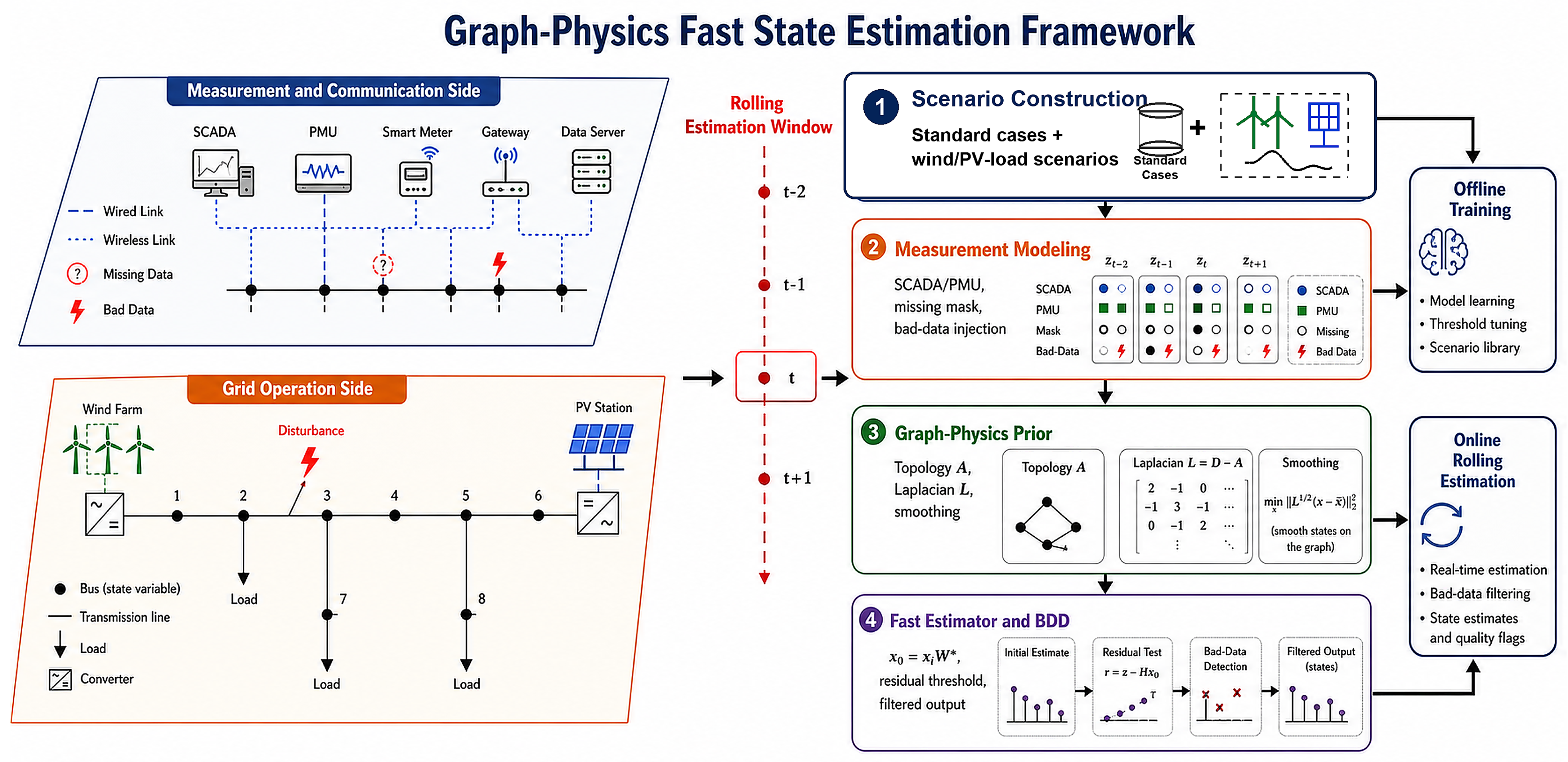
This section first gives the overall framework before introducing the feature mapping, residual screening, and algorithmic steps. Figure 1 is retained as the complete workflow diagram because it connects the sensing side, grid-operation side, offline calibration, graph topology prior, and online residual filtering in one view. For readability, the description below separates this overview into three functional layers, and the subsequent subsections give the mathematical details.

Figure 1. Overall framework of the proposed graph-physics-constrained fast state estimation method.

In Figure 1, the left layer gives the data and operating environment. The middle layer indicates the rolling estimation window at time t. The right layer gives the computational workflow: scenario construction, measurement modeling, graph–physics prior construction, and fast estimation with BDD. Offline training provides the scenario library, fast-mapping model, and residual threshold, whereas online rolling estimation performs real-time state estimation, bad data filtering, state-output generation, and quality-flag reporting. The detailed mathematical definitions corresponding to these modules are given in the following subsections. It should be emphasized that Figure 1 was initially prepared with the assistance of [ChatGPT-5.5]. We provided detailed textual instructions regarding the overall framework, key modules, technical workflow, and visual elements. The AI tool was not used to generate research data, simulation results, numerical analyses, or scientific conclusions.

The framework follows the logic of “operating scenario–model construction–online solution.” The scenario module provides multiple operating-point samples, the measurement modeling module converts wind/PV fluctuations, missing measurements, and bad data disturbances into trainable features, the graph–physics prior module provides topology constraints, and the fast estimator performs online state estimation and abnormal-measurement filtering. In this way, interpretable grid topology and residual detection mechanisms constrain the fast mapping process, strengthening the connection between learning-based estimators and conventional state-estimation workflows.

The phrase graph–physics-constrained is used in a limited and engineering-oriented sense: the physical prior is represented by the grid topology, branch-reactance-based Laplacian weights, and residual consistency with the measurement equation. It does not mean that all nonlinear AC power-flow equations are imposed as hard constraints in the current prototype.

3.1. Input Features and Fast Mapping

The proposed method adopts a fast estimation prototype enhanced by graph topology priors. The input feature vector consists of filled measurements, the missing mask, and anomaly scores:

$$\mathit{\xi }=\left[{\mathit{z}}_{\mathrm{fill}},\mathit{m},\mathit{s}\right].$$

(10)

In the offline stage, a ridge-regularized fast mapping learns the relationship from measurement features to state variables:

$${\mathit{W}}^{\ast }=arg\underset{\mathit{W}}{min}{∥\mathbf{\Phi }\mathit{W}-\mathit{X}∥}_F^2+\lambda {∥\mathit{W}∥}_F^2.$$

(11)

The online initial estimate is

$${\mathit{x}}_0={\mathit{\xi }}_t{\mathit{W}}^{\ast }.$$

(12)

The estimate is then corrected by a graph-smoothing matrix:

$${\mathit{x}}_s={\left(\mathit{I}+\gamma {\mathit{L}}_s\right)}^{-1}{\mathit{x}}_0.$$

(13)

Here, $\mathit{\xi }$ is the input feature vector, ${\mathit{z}}_{\mathrm{fill}}\in {\mathbb{R}}^M$ denotes available measurements after mean filling using the training-sample measurement mean, $\mathit{m}\in {\mathbb{R}}^M$ describes measurement availability, and $\mathit{s}\in {\mathbb{R}}^M$ denotes auxiliary anomaly scores computed only from online observable quantities. The matrix $\mathbf{\Phi }$ is the training feature matrix assembled from historical samples, $\mathit{X}$ is the corresponding training state matrix, $\mathit{W}$ is the mapping coefficient matrix, ${\mathit{W}}^{\ast }$ is the ridge-regularized optimal mapping, $\lambda$ is the ridge coefficient, and ${\parallel ·\parallel }_F$ is the Frobenius norm. The vector ${\mathit{\xi }}_t$ is the online feature vector at time t, ${\mathit{x}}_0$ is the initial online state estimate, ${\mathit{x}}_s$ is the graph-smoothed state estimate, $\gamma$ is the graph-smoothing coefficient, and $\mathit{I}$ is an identity matrix with the same dimension as ${\mathit{L}}_s$.

In the first pass, $s_i=|(z_i-{\mu }_i)/{\sigma }_i|m_i$, where $s_i$ is the ith anomaly score, $z_i$ is the ith measurement, ${\mu }_i$ is the training-sample mean of the ith measurement, and ${\sigma }_i$ is the corresponding noise standard deviation. In the second pass, $s_i$ is updated by the normalized residual score $|z_i-{\mathit{H}}_i{\mathit{x}}_0|/{\sigma }_i$, where ${\mathit{H}}_i$ is the ith row of $\mathit{H}$. The true bad data labels and the artificially injected bad data positions are not used as input features. The missing mask distinguishes true measurements from filled values, preserving the influence of the missing pattern on state estimation. The regularization term ${\lambda \parallel \mathit{W}\parallel }_F^2$ suppresses overfitting under limited training samples, especially when the state dimension increases in case300. The ridge coefficient $\lambda$ in the fast mapping is a separate hyperparameter from ${\lambda }_{\mathrm{WLS}}$ in the regularized WLS benchmark.

Mean filling is used here as a simple and reproducible baseline so that the contribution of the missing mask and graph topology prior can be isolated. More advanced imputation methods, such as graph-based interpolation, temporal reconstruction, or data-driven missing-measurement recovery, may further improve the estimator and will be considered in future work.

The graph-smoothing matrix converts branch topology into a post-processing constraint. For neighboring buses with strong electrical connections, state variables should not show abrupt changes that contradict power-flow regularity. The parameter $\gamma$ controls the tradeoff between the measurement-driven fast-mapping output and the graph-smoothing constraint. In the current simulation, $\gamma$ is selected as a fixed empirical value; it can be further calibrated by validation-set search or Bayesian optimization.

3.2. Bad Data Detection and Filtering

The measurements are reconstructed from the estimated state, and the normalized residual is computed as

$$r_i={\displaystyle \frac{\left|z_i-{\mathit{H}}_i{\mathit{x}}_s\right|}{{\sigma }_i}}.$$

(14)

Here, $r_i$ is the normalized residual of the ith measurement, $z_i$ is the observed measurement value, ${\mathit{H}}_i$ is the ith row of the measurement matrix, ${\mathit{x}}_s$ is the smoothed state estimate, and ${\sigma }_i$ is the standard deviation of the ith measurement noise.

If $r_i$ exceeds the threshold $\tau$ calibrated on the training set and the corresponding measurement is not missing, the measurement is marked as suspicious bad data:

$$b_i=\left\{\begin{array}{cc}1,\hfill & r_i>\tau \mathrm{and}{m}_i=1,\hfill \\ 0,\hfill & \mathrm{otherwise}.\hfill \end{array}\right.$$

(15)

Here, $b_i$ is the binary bad data flag of the ith measurement and $\tau$ is the residual threshold calibrated from the training data. The threshold is determined by maximizing the F1-score on the training set:

$${\tau }^{\ast }=arg\underset{\tau }{max}F1\left(\tau \right).$$

(16)

Here, ${\tau }^{\ast }$ is the selected optimal residual threshold and $F1\left(\tau \right)$ is the F1-score obtained when threshold $\tau$ is applied to the training residuals.

The filtering process follows the order of state estimation, residual judgment, and filtered output. This is consistent with conventional WLS residual detection, but the state initial value is produced by the calibrated fast mapping rather than an iterative solution at every sampling instant. This design reduces repeated online solution overhead and extends the calibration target from residual minimization to F1-score optimization, jointly considering false alarms and missed detections. Since renewable fluctuations may also cause measurement deviations, only valid measurements with $m_i=1$ are included in bad data judgment to avoid misclassifying missing measurements as bad data.

Residual-threshold detection is still a local abnormality-identification mechanism and may produce false alarms in small systems or samples with weak abnormal amplitudes. Therefore, the case studies report accuracy, false positive rate (FPR), false negative rate (FNR), and F1-score to fully characterize detection performance.

3.3. Evaluation Metrics and Complexity

The state estimation error is evaluated by phase-angle root mean square error (RMSE), voltage magnitude RMSE, mean absolute error (MAE), and maximum absolute error. These metrics are defined as  

$${\mathrm{RMSE}}_{\theta }=\sqrt{{\displaystyle \frac{1}{N-1}}\sum _{i=2}^N{\left({\theta }_i-{\widehat{\theta }}_i\right)}^2}.$$

(17)

$${\mathrm{RMSE}}_V=\sqrt{{\displaystyle \frac{1}{N}}\sum _{i=1}^N{\left(\Delta V_i-{\widehat{\Delta V}}_i\right)}^2},\mathrm{MAE}={\displaystyle \frac{1}{2N-1}}{\displaystyle \sum _{j=1}^{2N-1}}|x_j-{\widehat{x}}_j|,$$

(18)

$$\mathrm{MaxErr}=\underset{j}{max}|x_j-{\widehat{x}}_j|.$$

(19)

Here, ${\mathrm{RMSE}}_{\theta }$ is the phase-angle RMSE, ${\mathrm{RMSE}}_V$ is the voltage magnitude deviation RMSE, $\mathrm{MAE}$ is the mean absolute state error, and $\mathrm{MaxErr}$ is the maximum absolute state error. The variables ${\theta }_i$ and ${\widehat{\theta }}_i$ are the true and estimated phase angles of bus i, respectively; $\Delta V_i$ and ${\widehat{\Delta V}}_i$ are the true and estimated voltage magnitude deviations of bus i, respectively; and $x_j$ and ${\widehat{x}}_j$ are the jth components of the true and estimated state vectors $\mathit{x}$ and $\widehat{\mathit{x}}$.

Bad data detection performance is evaluated by accuracy, false positive rate, false negative rate, and F1-score:

$$F1={\displaystyle \frac{2·\mathrm{Precision}·\mathrm{Recall}}{\mathrm{Precision}+\mathrm{Recall}}}.$$

(20)

$$\mathrm{Accuracy}={\displaystyle \frac{TP+TN}{TP+TN+FP+FN}},\mathrm{FPR}={\displaystyle \frac{FP}{FP+TN}},\mathrm{FNR}={\displaystyle \frac{FN}{FN+TP}}.$$

(21)

Here, $\mathrm{Precision}=TP/(TP+FP)$, $\mathrm{Recall}=TP/(TP+FN)$, $TP$ is the number of true positives, $TN$ is the number of true negatives, $FP$ is the number of false positives, and $FN$ is the number of false negatives. $\mathrm{Accuracy}$, $\mathrm{FPR}$, and $\mathrm{FNR}$ denote the detection accuracy, false positive rate, and false negative rate, respectively.

The main online cost of WLS comes from matrix solution, whereas the online stage of the proposed method mainly includes feature normalization, matrix multiplication, and one graph-smoothing operation. The computational speedup is defined as

$$\mathrm{Speedup}={\displaystyle \frac{T_{\mathrm{WLS}}}{T_{\mathrm{fast}}}}.$$

(22)

Here, $T_{\mathrm{WLS}}$ is the online runtime of the WLS benchmark for one estimation sample, $T_{\mathrm{fast}}$ is the online runtime of the proposed fast estimator for the same sample, and $\mathrm{Speedup}$ is their runtime ratio.

From a computational perspective, WLS needs to form the gain matrix and solve a linear system at each time instant, and its complexity increases with the state and measurement dimensions. The proposed method transfers the main computation to the offline stage. Online, it performs feature normalization, one matrix mapping, one graph-smoothing operation, and one residual computation. If the state dimension is n and the feature dimension is p, the mapping cost is approximately $O\left(pn\right)$, where $n=2N-1$ and p is the length of $\mathit{\xi }$. In the present implementation, the smoothing operator ${(\mathit{I}+\gamma {\mathit{L}}_s)}^{-1}$ is precomputed offline and applied online as a fixed matrix operation; if a sparse iterative solver is used instead, the per-iteration smoothing cost is proportional to the number of nonzero Laplacian entries. Therefore, the reported timing results should be interpreted as implementation-specific online runtimes rather than as a universal asymptotic proof.

The offline stage includes scenario generation, ridge-mapping calibration, graph-smoothing matrix preparation, and residual-threshold search. This cost is paid once before online deployment and is updated only when the operating scenario library or bad data distribution is recalibrated. Therefore, the present experiments emphasize online rolling-estimation latency, while the offline burden is discussed as an implementation-dependent calibration cost rather than as a per-sample dispatch center runtime.

3.4. Algorithmic Procedure

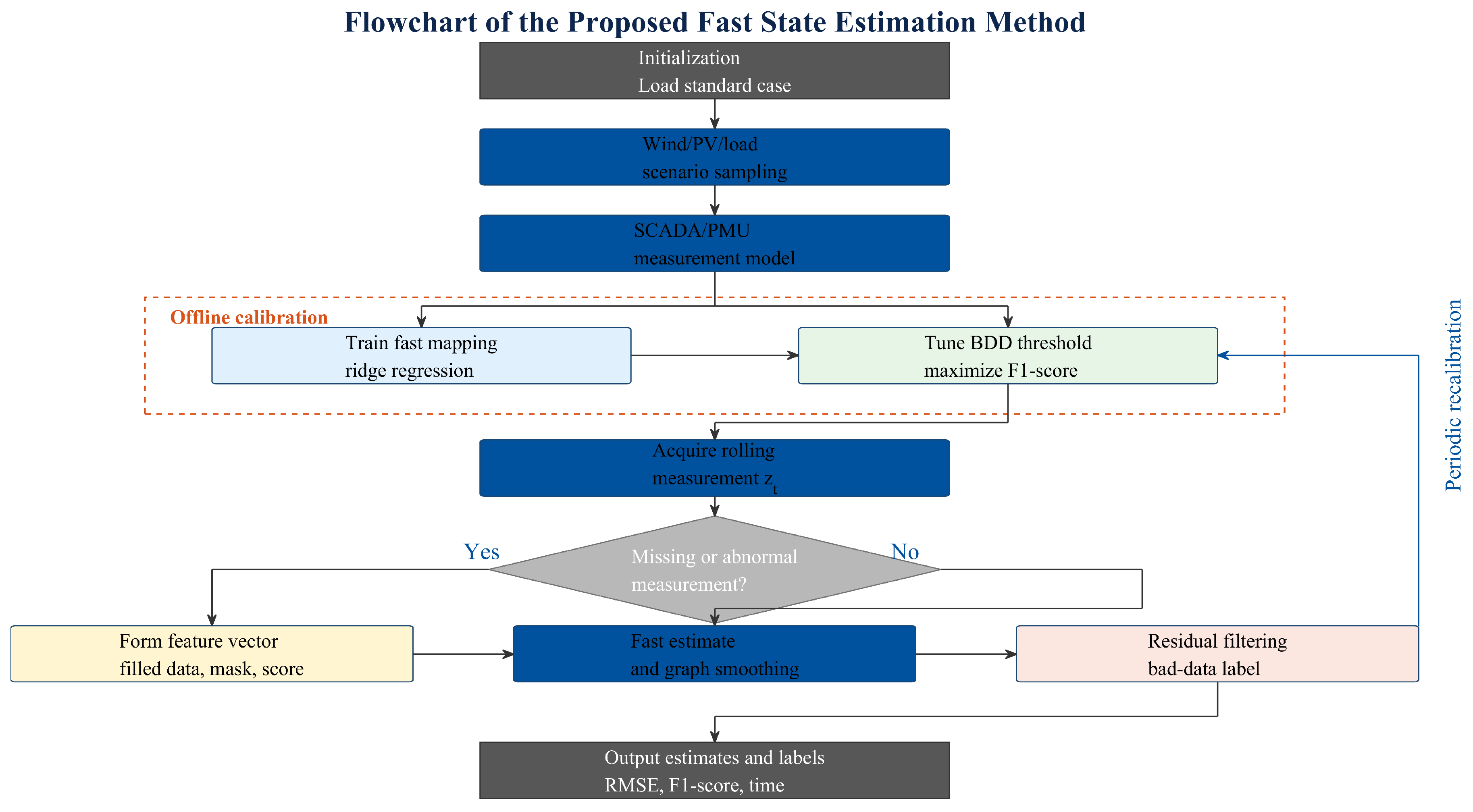
After defining the feature vector, residual criterion, and evaluation metrics, the complete offline–online execution sequence is summarized in Figure 2. The figure is intended to guide the reader through the training, threshold calibration, online state estimation, and bad data filtering stages before the pseudo-code is listed in Algorithm 1.

Figure 2. Flowchart of the proposed graph–physics-constrained fast state estimation method.

Figure 2 presents the execution sequence of the proposed method. The upper part corresponds to offline scenario construction and model calibration, including standard-case loading, wind/PV-load scenario sampling, hybrid-measurement construction, missing-data and bad data injection, fast-mapping training, and threshold search. The lower part corresponds to online rolling estimation, including feature assembly, fast-forward mapping, graph smoothing, residual detection, and filtered output. Unlike WLS, which requires matrix solutions at every time instant, this procedure concentrates online computation on fixed-dimension matrix operations and is therefore suitable for high-frequency rolling estimation. The arrow from offline training to online estimation indicates that ${\mathit{W}}^{\ast }$ and ${\tau }^{\ast }$ are reused. The feedback arrow from online estimation to model calibration indicates that the parameters can be recalibrated using new samples when operating scenarios or bad data distributions change. The detailed procedure is summarized in Algorithm 1.

Algorithm 1 Pseudo-code of the proposed fast state estimation algorithm.

Input: Standard test system, missing rate $r_m$, bad-data ratio $r_b$, renewable penetration $\rho$, regularization coefficient $\lambda$, graph-smoothing coefficient $\gamma$, and residual threshold candidates. Output: State estimate $\widehat{\mathit{x}}$, bad-data label $\widehat{\mathit{b}}$, RMSE, F1-score, and online computation time.   1: Initialize $\mathit{H}$ and ${\mathit{L}}_s$ from case39, case118, or case300.   2: Generate wind/PV/load scenarios and construct SCADA/PMU measurement samples.   3: Inject missing masks and bad-data disturbances according to $r_m$ and $r_b$.   4: Build the training feature matrix $\mathbf{\Phi }=[{\mathit{z}}_{\mathrm{fill}},\mathit{m},\mathit{s}]$.   5: Estimate the fast mapping ${\mathit{W}}^{\ast }={({\mathbf{\Phi }}^T\mathbf{\Phi }+\lambda \mathit{I})}^{-1}{\mathbf{\Phi }}^T\mathit{X}$.   6: Calibrate ${\tau }^{\ast }=arg{max}_{\tau }F1\left(\tau \right)$ on the training set.   7: for each online rolling sample ${\mathit{z}}_t$ do   8:       Form ${\mathit{\xi }}_t=[{\mathit{z}}_{\mathrm{fill},t},{\mathit{m}}_t,{\mathit{s}}_t]$ and calculate ${\mathit{x}}_0={\mathit{\xi }}_t{\mathit{W}}^{\ast }$.   9:       Apply graph smoothing ${\mathit{x}}_s={(\mathit{I}+\gamma {\mathit{L}}_s)}^{-1}{\mathit{x}}_0$. 10:       Reconstruct measurements and compute normalized residuals $r_i$. 11:       if $r_i>{\tau }^{\ast }$ and $m_i=1$ then set ${\widehat{b}}_i=1$; otherwise set ${\widehat{b}}_i=0$. 12:       Output $\widehat{\mathit{x}}={\mathit{x}}_s$ and the filtered bad-data labels $\widehat{\mathit{b}}$. 13: end for 14: Compare FastGraphPhysics with WLS and Huber robust WLS in terms of RMSE, F1-score, and online computation time.

4. Case Studies

4.1. Test Systems and Parameter Settings

The simulations use MATPOWER 8.1 case39, case118, and case300 standard systems [25,26]. These three systems represent small-, medium-, and relatively large-scale transmission networks, respectively, and are used to observe how algorithm performance changes with system size. Wind, PV, and load disturbance scenarios are constructed in each system, and WLS, Huber robust WLS, and FastGraphPhysics are compared on the same test samples. The numbers of training samples are 600, 500, and 360, and the numbers of test samples are 80, 60, and 40. To reduce dependence on a single random draw, all main experiments are repeated over five random seeds. Tables report mean values with standard deviations over these five runs. The baseline settings are a renewable penetration of 30%, a missing-measurement rate of 10%, a bad data ratio of 5%, a WLS regularization term of ${10}^{-4}$, a fast-mapping ridge coefficient of ${10}^{-2}$, and a graph-smoothing coefficient of $2\times {10}^{-2}$.

For reproducibility, renewable buses are sampled from non-reference buses with an above-median base load, with a count of approximately 15% of system buses. PMU buses are sampled from non-reference buses with a count of approximately 10% of system buses. The mixed measurement vector contains active power injection measurements for non-reference buses, active power branch-flow measurements for all active branches, voltage magnitude deviation measurements for all buses, and phase-angle measurements at selected PMU buses. The measurement-noise standard deviations are 0.010 for active power injection and flow measurements, 0.003 for voltage-deviation measurements, and 0.001 for PMU angle measurements. Load scaling follows $U(0.90,1.10)$, and renewable scaling is generated from a truncated normal-like factor $max(0,0.30+0.70u+0.10\eta )$ with $u\sim U(0,1)$ and $\eta \sim N(0,1)$. The missing values are filled by the training-sample measurement mean, while the mask $\mathit{m}$ is retained as an explicit input feature. The residual threshold $\tau$ is selected from 3:0.5:25 by maximizing the F1-score on the training set. All simulations are implemented in MATLAB R2024b using MATPOWER 8.1, with online time measured by MATLAB estimator calls.

The case studies focus on three questions. First, whether the fast mapping can maintain acceptable state estimation errors under different system sizes. Second, whether the residual-threshold mechanism can identify abnormal measurements when missing measurements and bad data coexist. Third, whether the online computation time grows more slowly than WLS when the system size increases from case39 to case300. To avoid misleading conclusions from a single metric, the state estimation part reports phase-angle RMSE, voltage RMSE, MAE, and maximum error; the bad data detection part reports accuracy, false positive rate, false negative rate, and F1-score; and the computation-efficiency part reports absolute time, speedup, and saved-time ratio.

4.2. State Estimation Accuracy

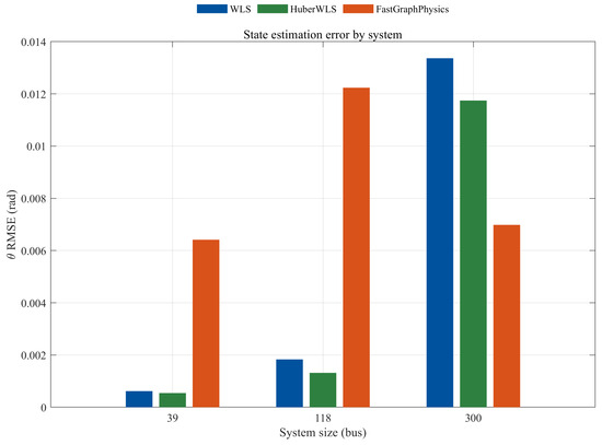
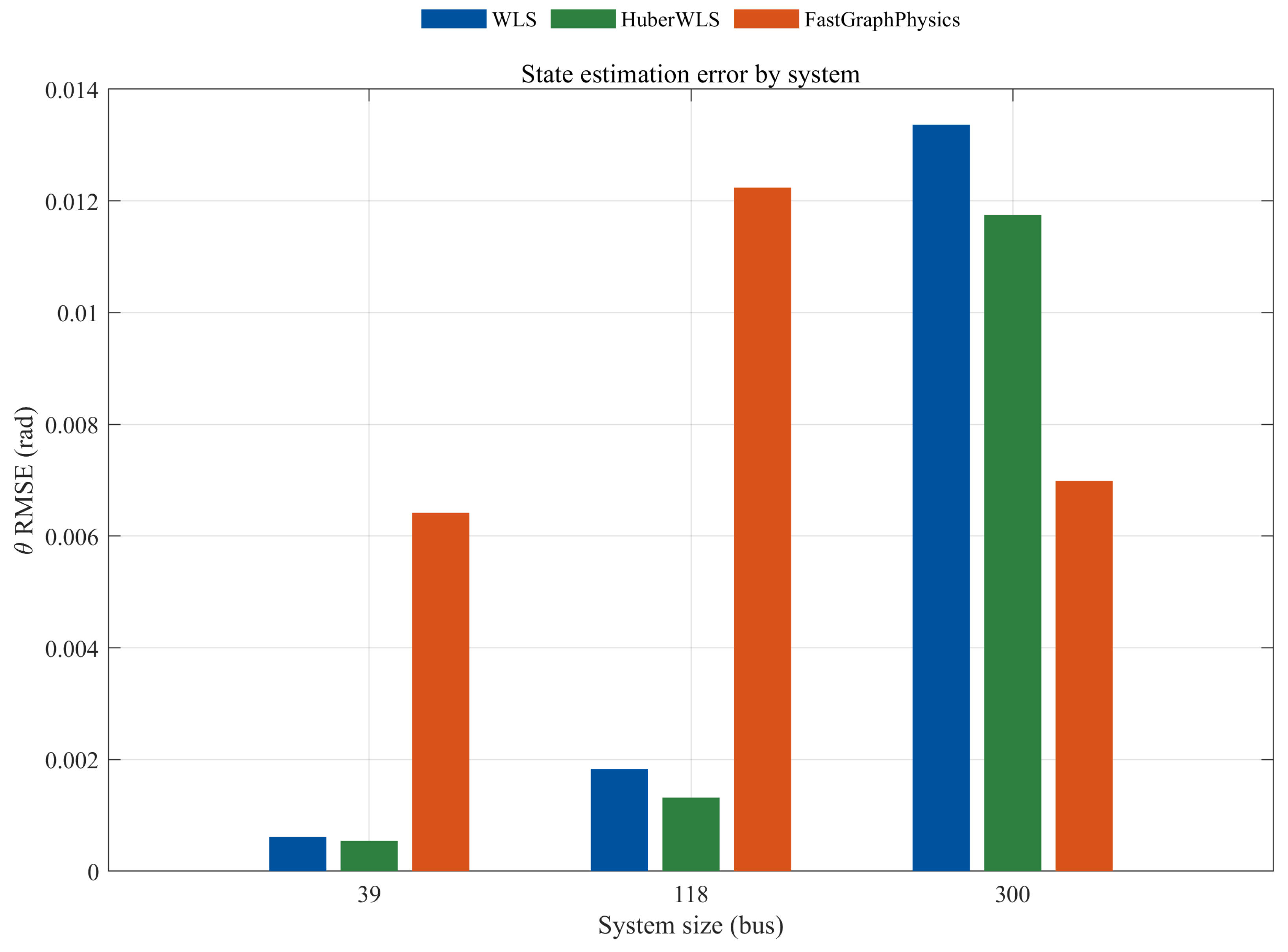
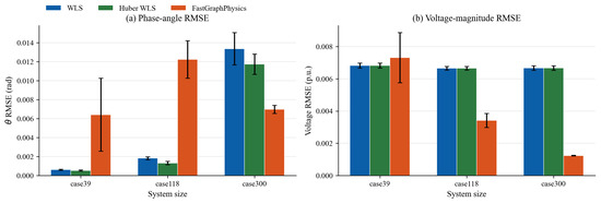
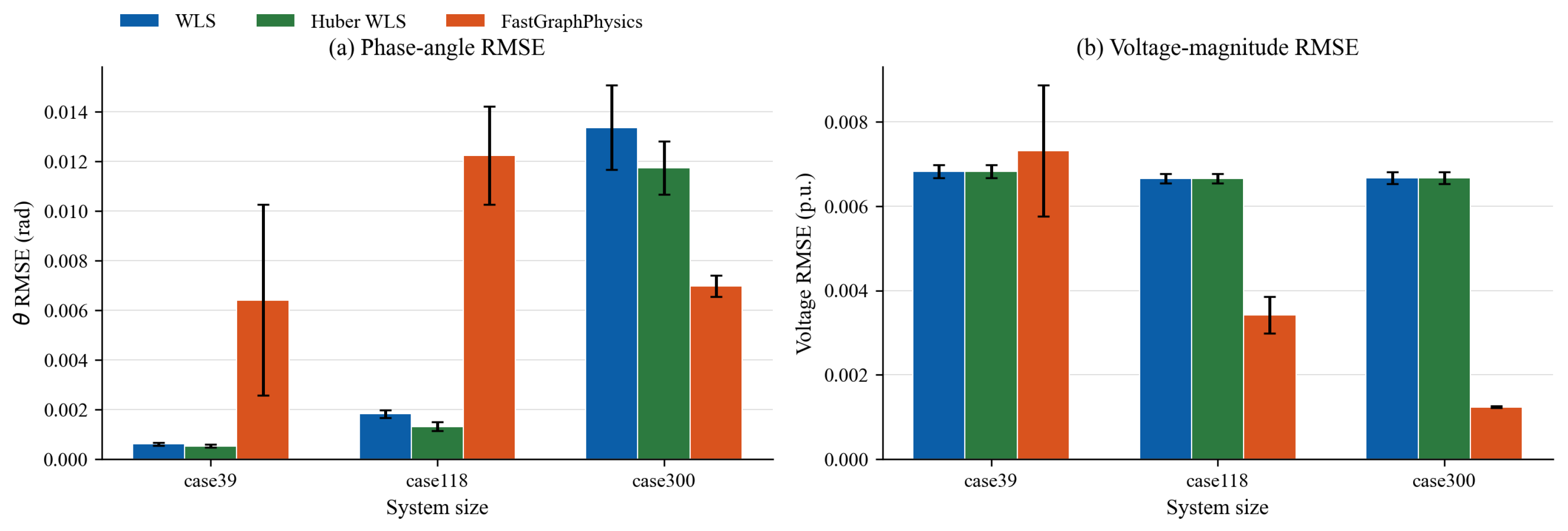
This subsection evaluates estimation accuracy before discussing bad data detection and computation time. Table 1 reports the numerical error metrics, Figure 3 visualizes phase-angle RMSE across system sizes, and Figure 4 summarizes multiple error indicators in one comparison.

Table 1. State estimation errors in standard test systems.

System	Method	$\mathit{\theta }$ RMSE	Voltage RMSE	MAE	Max. Error
39	WLS	$0.00062\pm 0.00006$	$0.00682\pm 0.00016$	$0.00218\pm 0.00005$	$0.04280\pm 0.00364$
39	Huber WLS	$0.00054\pm 0.00006$	$0.00682\pm 0.00016$	$0.00216\pm 0.00005$	$0.04280\pm 0.00364$
39	FastGraphPhysics	$0.00642\pm 0.00384$	$0.00731\pm 0.00155$	$0.00547\pm 0.00192$	$0.03015\pm 0.01007$
118	WLS	$0.00183\pm 0.00016$	$0.00665\pm 0.00011$	$0.00251\pm 0.00006$	$0.05143\pm 0.02276$
118	Huber WLS	$0.00132\pm 0.00018$	$0.00665\pm 0.00011$	$0.00233\pm 0.00003$	$0.05143\pm 0.02276$
118	FastGraphPhysics	$0.01224\pm 0.00197$	$0.00342\pm 0.00044$	$0.00602\pm 0.00059$	$0.06026\pm 0.01804$
300	WLS	$0.01337\pm 0.00170$	$0.00666\pm 0.00014$	$0.00341\pm 0.00014$	$0.37667\pm 0.08859$
300	Huber WLS	$0.01175\pm 0.00107$	$0.00666\pm 0.00014$	$0.00309\pm 0.00008$	$0.41190\pm 0.07075$
300	FastGraphPhysics	$0.00698\pm 0.00043$	$0.00124\pm 0.00002$	$0.00225\pm 0.00018$	$0.08058\pm 0.01125$

Figure 3. Grouped phase-angle RMSE comparison under different system sizes.

Figure 4. Comprehensive state-estimation error comparison, including phase-angle RMSE, voltage RMSE, MAE, and maximum absolute error.

Table 1, Figure 3 and Figure 4 report the state estimation errors under different system sizes. Figure 3 separately plots the phase-angle RMSE using grouped bars to highlight the difference among WLS, Huber WLS, and the fast method as the system size changes.

The numerical results show that WLS and Huber WLS still achieve lower phase-angle error in case39 and case118, which is consistent with the stable behavior of model-based estimators in small and medium systems with sufficient measurement redundancy. In case39, the proposed method has a lower maximum error than WLS but a higher phase-angle RMSE and MAE, indicating that the fast mapping can suppress some extreme errors but remains sensitive to global angle bias in small systems. In case118, the voltage RMSE of the fast method is lower than that of WLS, while the phase-angle RMSE is higher. In case300, the proposed method achieves lower phase-angle RMSE, voltage RMSE, MAE, and maximum error than both WLS and Huber WLS. These results indicate that the present fast linearized prototype is most useful in the larger case300 scenario, whereas WLS or robust WLS should still be retained when small-system phase-angle accuracy is the primary requirement.

The stronger relative performance in the larger system can be explained from both statistical and topological perspectives. In case39 and case118, a small number of missing or abnormal measurements can noticeably bias the learned linear mapping, and the graph-smoothing prior has fewer neighboring constraints from which to recover local consistency. In case300, the measurement vector and the network graph contain more redundant local relations. Because the injected bad data are randomly distributed, most abnormal measurements appear as sparse local inconsistencies rather than as coordinated changes over an entire electrically connected region. The Laplacian prior can therefore average local noise and suppress isolated nonphysical jumps more effectively, while the residual threshold has a larger population of normal and abnormal residuals from which to separate the two classes. This does not prove that the method will always improve with system size; it explains why, under the present random-error and standard-case settings, the relative benefit is clearer in case300.

4.3. Bad Data Detection Performance

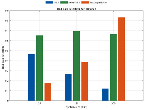
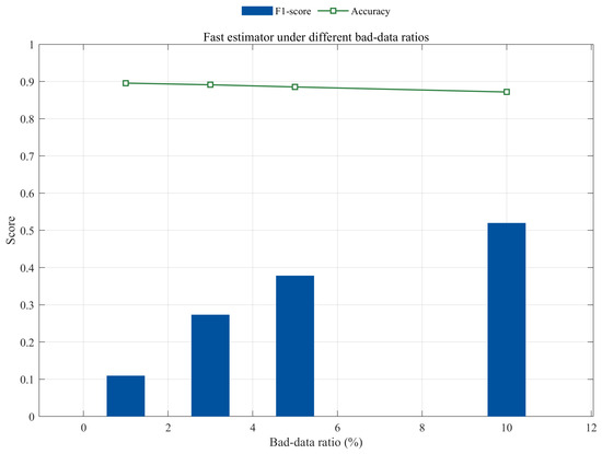
This subsection evaluates whether abnormal measurements can be identified after state estimation. Table 2 first compares WLS, Huber WLS, and the proposed fast method; Figure 5 visualizes F1-score differences; Table 3 and Figure 6 then examine the sensitivity to different bad data ratios; and Figure 7 summarizes FPR, FNR, accuracy, and F1-score.

Table 2. Bad data detection performance.

System	Method	Accuracy	FPR	FNR	F1-Score
39	WLS	$0.9642\pm 0.0019$	$0.0013\pm 0.0004$	$0.6889\pm 0.0246$	$0.4654\pm 0.0303$
39	Huber WLS	$0.9725\pm 0.0022$	$0.0033\pm 0.0003$	$0.4865\pm 0.0309$	$0.6515\pm 0.0281$
39	FastGraphPhysics	$0.6941\pm 0.0368$	$0.3040\pm 0.0438$	$0.3435\pm 0.1011$	$0.1767\pm 0.0103$
118	WLS	$0.9582\pm 0.0019$	$0.0000\pm 0.0000$	$0.8452\pm 0.0059$	$0.2679\pm 0.0089$
118	Huber WLS	$0.9756\pm 0.0015$	$0.0029\pm 0.0004$	$0.4377\pm 0.0134$	$0.6948\pm 0.0114$
118	FastGraphPhysics	$0.8893\pm 0.0080$	$0.1008\pm 0.0095$	$0.3022\pm 0.0272$	$0.3838\pm 0.0139$
300	WLS	$0.9534\pm 0.0014$	$0.0000\pm 0.0000$	$0.9356\pm 0.0020$	$0.1210\pm 0.0036$
300	Huber WLS	$0.9732\pm 0.0011$	$0.0036\pm 0.0004$	$0.4696\pm 0.0080$	$0.6630\pm 0.0054$
300	FastGraphPhysics	$0.9816\pm 0.0029$	$0.0144\pm 0.0036$	$0.0936\pm 0.0222$	$0.8316\pm 0.0190$

Figure 5. Grouped F1-score comparison of bad data detection under different system sizes.

Table 3. Detection performance under different bad data ratios in case118.

Bad Data Ratio	Accuracy	FPR	FNR	F1-Score
1%	$0.8956\pm 0.0091$	$0.1023\pm 0.0095$	$0.3258\pm 0.0289$	$0.1096\pm 0.0102$
3%	$0.8911\pm 0.0063$	$0.1027\pm 0.0067$	$0.3106\pm 0.0289$	$0.2735\pm 0.0124$
5%	$0.8853\pm 0.0117$	$0.1046\pm 0.0135$	$0.3063\pm 0.0312$	$0.3783\pm 0.0124$
10%	$0.8718\pm 0.0046$	$0.1074\pm 0.0066$	$0.3131\pm 0.0257$	$0.5199\pm 0.0115$

Figure 6. Detection performance under different bad data ratios on a common 0–1 score axis; bars denote F1-score and the curve denotes accuracy.

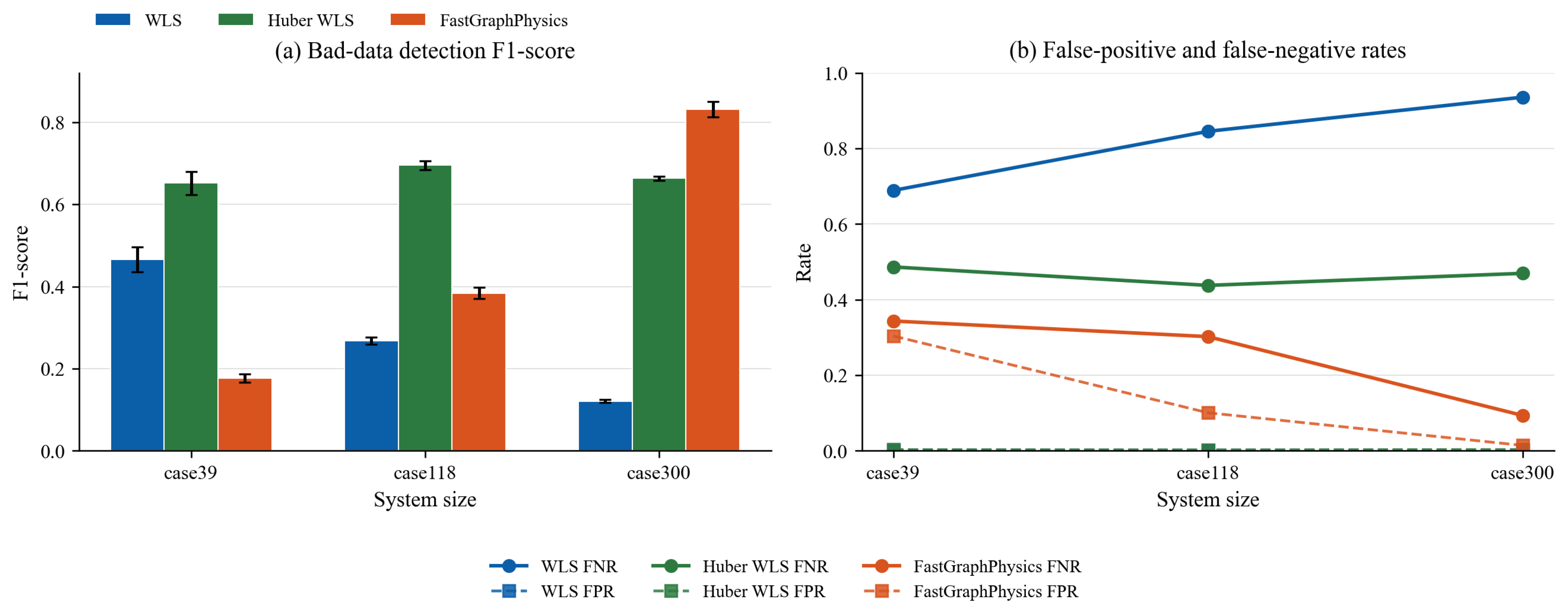
Figure 7. Simplified bad data detection comparison, including F1-score and the false-positive/false-negative tradeoff under different system sizes.

Table 2, Figure 5 and Figure 7 report the bad data detection performance. Figure 5 directly compares F1-scores in the three standard systems, highlighting the variation in detection performance with system size. Figure 6 jointly presents the bad data ratio scan in case118 using bars and an accuracy curve. Figure 7 includes F1-score together with FPR and FNR; the latter two are the error types that determine the detection tradeoff.

Table 2 shows that WLS has high accuracy in all three systems, but its F1-score decreases as the system size increases, reaching only $0.1210\pm 0.0036$ in case300. This is because accuracy is easily dominated by the large number of normal measurements, while F1-score better reflects the ability to identify bad data samples. Huber WLS improves F1-score relative to WLS in all three systems, confirming the value of adding a robust baseline. The proposed fast method is not uniformly better: in case39, its F1-score is low because of a high false positive rate. In case118, it improves over WLS but remains weaker than Huber WLS. In case300, however, the F1-score reaches $0.8316\pm 0.0190$, and the false negative rate decreases to $0.0936\pm 0.0222$, indicating that graph smoothing and threshold calibration can enhance residual separability in the larger-scale scenario.

The improvement in case300 is also related to the residual distribution. In larger networks, the number of measurements increases and the random bad data samples occupy a relatively sparse subset of the complete measurement set. A topology-smoothed state estimate tends to make normal measurements cluster more tightly around the reconstructed measurement equation, whereas isolated abnormal measurements retain larger normalized residuals. This increases the separability between normal and abnormal residuals and reduces the false-negative rate of the proposed method in case300. By contrast, in smaller systems, fewer measurements are available for threshold calibration, and a small number of biased estimates may produce many false alarms. This explains why the proposed mapping is relatively more effective in the larger benchmark, but it also confirms that the method is not yet a general cyber-security detector.

The present bad data validation uses randomly injected gross errors to test whether the estimator can identify unstructured abnormal measurements under stochastic renewable operating points. Coordinated false-data injection attacks are more demanding because they may be constructed to evade residual-based detection. Therefore, cyber-attack-oriented validation is treated as a future extension rather than as a claim of complete cyber-security defense in this linearized prototype.

The non-stacked FPR/FNR panel in Figure 7 further indicates that bad data detection performance depends on the tradeoff between false alarms and missed detections rather than accuracy alone. FPR and FNR are shown separately because they have different denominators. For online dispatch, missed detections may allow erroneous states to enter subsequent security analysis, whereas false alarms may increase manual review or measurement-removal costs. Therefore, this paper uses F1-score as the threshold-calibration objective to jointly constrain false alarms and missed detections.

Figure 6 shows that when the bad data ratio in case118 increases from 1% to 10%, the F1-score generally increases, while the accuracy changes only slightly. This phenomenon suggests that when the abnormal ratio is low, a small number of bad data samples can be masked by normal fluctuations. When the abnormal ratio increases, the residual distribution becomes more distinguishable, and threshold detection becomes more stable. The 5% sweep result is generated from the same multi-seed protocol as the main tables, but the sweep uses a dedicated case118 sensitivity dataset; therefore, it is interpreted as a sensitivity trend rather than as a duplicate of the main case118 row in Table 2.

4.4. Online Computation Efficiency

This subsection reports the online computation efficiency after the accuracy and detection results. Table 4 lists the average online time and speedup, while Figure 8 visualizes both absolute runtime and acceleration trends.

Table 4. Average online computation time in standard test systems.

System	Method	Time/ms	Speedup Over WLS
39	WLS	$1.112\pm 0.100$	-
39	Huber WLS	$2.134\pm 0.150$	$0.52$
39	FastGraphPhysics	$0.219\pm 0.079$	$5.53$
118	WLS	$7.383\pm 0.413$	-
118	Huber WLS	$11.848\pm 0.354$	$0.62$
118	FastGraphPhysics	$0.389\pm 0.100$	$19.95$
300	WLS	$66.063\pm 3.054$	-
300	Huber WLS	$96.081\pm 1.070$	$0.69$
300	FastGraphPhysics	$1.922\pm 0.374$	$35.08$

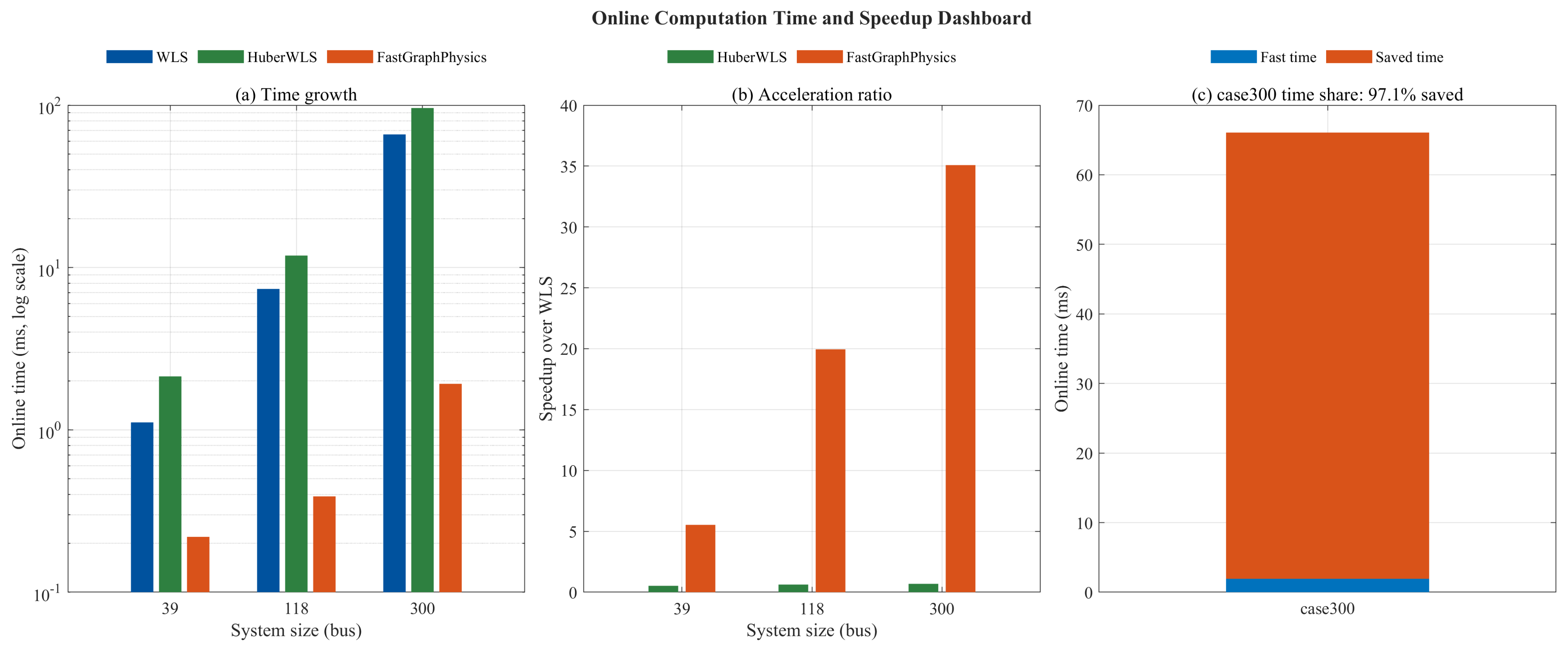
Figure 8. Online computation time and speedup comparison.

Table 4 and Figure 8 show the online computation time under different system sizes. Figure 8a uses logarithmic coordinates to display the average online time of WLS and the fast method. Figure 8b gives the speedup over WLS, and Figure 8c shows the actual fast-method time and saved-time share in case300. The results indicate that acceleration is reflected not only in absolute time reduction but also in the scaling difference relative to WLS.

The average online times of the fast method in case39, case118, and case300 are $0.219\pm 0.079$ ms, $0.389\pm 0.100$ ms, and $1.922\pm 0.374$ ms, respectively. The corresponding speedups over WLS are approximately 5.53, 19.95, and 35.08. Huber WLS improves robustness but has higher online runtime than WLS because of the iterative reweighting procedure. As the system size increases, WLS and Huber WLS need to process higher state and measurement dimensions, so the matrix solution overhead rises rapidly. In contrast, the online stage of the fast method mainly performs feature normalization, matrix mapping, residual computation, and graph smoothing with a fixed computational path. In case300, the average WLS time is $66.063\pm 3.054$ ms, while the fast-method time is $1.922\pm 0.374$ ms, indicating that the proposed method is suitable for high-frequency rolling estimation scenarios when the larger-system operating condition is relevant.

The system-size effect is therefore most direct in computation. WLS repeatedly assembles and solves a weighted least-squares problem for each online sample, and the cost of the linear solve grows rapidly with the number of states and active measurements. The proposed method moves the fitting of the mapping, the smoothing operator, and the threshold calibration to the offline stage. During online deployment, the main operations are fixed matrix multiplication, residual evaluation, and application of a precomputed smoothing operator. These operations still grow with system size, but in the present implementation they grow more gently than repeated WLS solves. Consequently, the relative speedup becomes larger as the benchmark system increases from case39 to case300.

Combining Table 1 and Table 4, the advantage of the proposed method mainly appears under large-scale, online, and high-frequency conditions, and it does not constitute a full-metric replacement for WLS. For dispatch center online monitoring, if estimation frequency is the primary bottleneck, the fast method can serve as a front-end fast estimator or abnormality screener for WLS. If a small system requires high phase-angle accuracy, WLS or AC state estimation should still be retained as the final check.

5. Conclusions

This paper has studied fast state estimation for wind/PV integrated transmission networks under missing measurements and bad data contamination. A graph–physics-constrained fast state estimation method has been proposed. The method constructs a graph Laplacian prior from network topology and combines fast mapping, graph smoothing, and residual detection to achieve online state estimation and bad data filtering. Multi-seed simulation results show that the proposed method reduces online computation time in case39, case118, and case300. In case300, the average online time decreases from $66.063\pm 3.054$ ms for WLS to $1.922\pm 0.374$ ms. The method also achieves an F1-score of $0.8316\pm 0.0190$ for bad data detection in case300. The relative advantage in case300 is attributed to two factors: the online computation of the fast mapping grows more gently than repeated WLS solves, and the larger graph provides more redundant local topology and measurement relations for smoothing and residual separation. However, the evidence remains limited to three standard benchmark systems with simulated renewable scenarios and randomly injected gross errors. Its accuracy and BDD performance are scenario dependent: WLS and Huber WLS remain more reliable for phase-angle accuracy in smaller systems, and Huber WLS provides stronger BDD performance in case39 and case118. Therefore, the proposed method should be viewed as a preliminary proof-of-concept for a fast large-scale rolling estimator or abnormality screener, rather than a universal replacement for robust model-based state estimation.

Future work will proceed in three directions. First, the linearized model will be extended to a full AC state estimation model. Second, the fast mapping will be replaced by a trainable message-passing GNN. Third, practical measurement data, topology changes, and cyber-attack-type bad data scenarios will be introduced to further validate engineering applicability.

References

- Schweppe, F.C.; Wildes, J. Power system static-state estimation, Part I: Exact model. IEEE Trans. Power Appar. Syst. 1970, PAS-89, 120–125. [Google Scholar] [CrossRef] [Scilit]
- Monticelli, A. Electric power system state estimation. Proc. IEEE 2000, 88, 262–282. [Google Scholar] [CrossRef] [Scilit]
- Abur, A.; Gómez-Expósito, A. Power System State Estimation; CRC Press: Boca Raton, FL, USA, 2004. [Google Scholar] [CrossRef] [Scilit]
- Cheng, G.; Lin, Y.; Abur, A.; Gómez-Expósito, A.; Wu, W. A survey of power system state estimation using multiple data sources: PMUs, SCADA, AMI, and beyond. IEEE Trans. Smart Grid 2024, 15, 1129–1151. [Google Scholar] [CrossRef] [Scilit]
- Chen, H.; Zhang, L.; Mo, J.; Martin, K.E. Synchrophasor-based real-time state estimation and situational awareness system for power system operation. J. Mod. Power Syst. Clean. Energy 2016, 4, 370–382. [Google Scholar] [CrossRef] [Scilit]
- Jin, T.; Shen, X. A mixed WLS power system state estimation method integrating a wide-area measurement system and SCADA technology. Energies 2018, 11, 408. [Google Scholar] [CrossRef] [Scilit]
- Cho, Y.-S.; Choi, Y.-H. Methodology for implementing the state estimation in renewable energy management systems. Energies 2021, 14, 2301. [Google Scholar] [CrossRef] [Scilit]
- Qing, H.; Singh, A.K.; Batzelis, E. Review on distribution system state estimation considering renewable energy sources. Energies 2025, 18, 2524. [Google Scholar] [CrossRef] [Scilit]
- Lopez-Ramirez, I.; Rodriguez-Seco, J.E.; Zamora, I. Assessment on power systems non-deterministic state estimation algorithms. Electr. Power Syst. Res. 2023, 214, 108880. [Google Scholar] [CrossRef] [Scilit]
- Mili, L.; Phaniraj, V.; Rousseeuw, P.J. Least median of squares estimation in power systems. IEEE Trans. Power Syst. 1991, 6, 511–523. [Google Scholar] [CrossRef] [Scilit] [PubMed]
- Gol, M.; Abur, A. LAV based robust state estimation for systems measured by PMUs. IEEE Trans. Smart Grid 2014, 5, 1808–1814. [Google Scholar] [CrossRef] [Scilit]
- Liu, Y.; Ning, P.; Reiter, M.K. False data injection attacks against state estimation in electric power grids. ACM Trans. Inf. Syst. Secur. 2011, 14, 1–33. [Google Scholar] [CrossRef] [Scilit]
- Kosut, O.; Jia, L.; Thomas, R.J.; Tong, L. Malicious data attacks on the smart grid. IEEE Trans. Smart Grid 2011, 2, 645–658. [Google Scholar] [CrossRef] [Scilit]
- Hug, G.; Giampapa, J.A. Vulnerability assessment of AC state estimation with respect to false data injection cyber-attacks. IEEE Trans. Smart Grid 2012, 3, 1362–1370. [Google Scholar] [CrossRef] [Scilit]
- Deng, R.; Xiao, G.; Lu, R.; Liang, H.; Vasilakos, A.V. False data injection on state estimation in power systems: Attacks, impacts, and defense: A survey. IEEE Trans. Ind. Inform. 2017, 13, 411–423. [Google Scholar] [CrossRef] [Scilit]
- Kipf, T.N.; Welling, M. Semi-supervised classification with graph convolutional networks. In Proceedings of the International Conference on Learning Representations, Toulon, France, 24–26 April 2017. [Google Scholar]
- Wu, Z.; Pan, S.; Chen, F.; Long, G.; Zhang, C.; Yu, P.S. A comprehensive survey on graph neural networks. IEEE Trans. Neural Netw. Learn. Syst. 2021, 32, 4–24. [Google Scholar] [CrossRef] [Scilit] [PubMed]
- Raissi, M.; Perdikaris, P.; Karniadakis, G.E. Physics-informed neural networks: A deep learning framework for solving forward and inverse problems involving nonlinear partial differential equations. J. Comput. Phys. 2019, 378, 686–707. [Google Scholar] [CrossRef] [Scilit]
- Karniadakis, G.E.; Kevrekidis, I.G.; Lu, L.; Perdikaris, P.; Wang, S.; Yang, L. Physics-informed machine learning. Nat. Rev. Phys. 2021, 3, 422–440. [Google Scholar] [CrossRef] [Scilit]
- de Jongh, S.; Gielnik, F.; Mueller, F.; Schmit, L.; Suriyah, M.; Leibfried, T. Physics-informed geometric deep learning for inference tasks in power systems. Electr. Power Syst. Res. 2022, 211, 108362. [Google Scholar] [CrossRef] [Scilit]
- Ngo, Q.-H.; Nguyen, B.L.H.; Vu, T.V.; Zhang, J.; Ngo, T. Physics-informed graphical neural network for power system state estimation. Appl. Energy 2024, 358, 122602. [Google Scholar] [CrossRef] [Scilit]
- Li, P.; Dai, Z.; Wang, Z.; Yu, Y. Spatio-temporal dynamic graph neural network-based missing measurement recovery method for power system state estimation. Appl. Energy 2026, 411, 127604. [Google Scholar] [CrossRef] [Scilit]
- Tian, G.; Gu, Y.; Shi, D.; Fu, J.; Yu, Z.; Zhou, Q. Neural-network-based power system state estimation with extended observability. J. Mod. Power Syst. Clean. Energy 2021, 9, 1043–1053. [Google Scholar] [CrossRef] [Scilit]
- Habib, B.; Isufi, E.; van Breda, W.; Jongepier, A.; Cremer, J.L. Deep statistical solver for distribution system state estimation. IEEE Trans. Power Syst. 2024, 39, 4039–4050. [Google Scholar] [CrossRef] [Scilit]
- Zimmerman, R.D.; Murillo-Sánchez, C.E.; Thomas, R.J. MATPOWER: Steady-state operations, planning, and analysis tools for power systems research and education. IEEE Trans. Power Syst. 2011, 26, 12–19. [Google Scholar] [CrossRef] [Scilit]
- Zimmerman, R.D.; Murillo-Sánchez, C.E. MATPOWER User’s Manual. Zenodo. 2025. Available online: https://matpower.org/docs/MATPOWER-manual-8.1.pdf (accessed on 15 June 2026).
Disclaimer/Publisher’s Note: The statements, opinions and data contained in all publications are solely those of the individual author(s) and contributor(s) and not of MDPI and/or the editor(s). MDPI and/or the editor(s) disclaim responsibility for any injury to people or property resulting from any ideas, methods, instructions or products referred to in the content. |
© 2026 by the authors. Licensee MDPI, Basel, Switzerland. This article is an open access article distributed under the terms and conditions of the Creative Commons Attribution (CC BY) license.