Multi-Resolution Acoustic Prototype Anchoring for Limited-Sample Industrial Anomalous Sound Detection

Abstract

Industrial anomalous sound detection is important for machine condition monitoring, especially when anomalous recordings are unavailable and only a small number of normal recordings can be collected from the target machine. This paper proposes target-domain cosine prototype anchoring (TD-CPA), a lightweight and interpretable framework for limited-sample industrial anomalous sound detection. The method combines multi-resolution Log-Mel representations with global, temporal-delta, and segment-wise statistical features to characterize both stable operating patterns and short-duration acoustic variations. PCA is then used to obtain compact embeddings, while ten target-normal recordings are employed to construct a target acoustic prototype. Anomaly scores are calculated based on the cosine deviation between each test embedding and this prototype. Experiments covering seven industrial machine categories show that TD-CPA achieves mean AUC, pAUC, and HScore values of 0.6067, 0.1389, and 0.2095, respectively, representing the highest numerical mean performance among the evaluated statistical, distance-based, compact autoencoder, and frozen pretrained-embedding baselines. Ablation experiments confirm the complementary contributions of the statistical feature components and multiple time-frequency resolutions. The target-sample sensitivity experiment further demonstrates that broader target-normal coverage generally improves detection performance. Overall, TD-CPA provides a simple, normal-data-only, and interpretable solution for industrial anomalous sound detection under limited target-data conditions.

1. Introduction

Reliable condition monitoring is essential for maintaining the safe and stable operation of industrial equipment. Among commonly used monitoring signals, such as vibration, current, temperature, and acoustic emission, sound has the advantages of non-contact acquisition, convenient sensor deployment, and continuous monitoring without interrupting machine operation. Changes in operating conditions, mechanical degradation, friction, impacts, and other abnormal events may alter the temporal or spectral characteristics of machine sounds. In practice, however, representative fault recordings are often difficult to collect, while only a small number of normal recordings may be available from a newly deployed target machine [1,2]. This creates a practical need for anomaly detection methods that can establish a reliable normal reference from limited target-domain data.

Anomalous sound detection (ASD) addresses this problem by learning normal acoustic characteristics and assigning higher anomaly scores to recordings that deviate from the learned normal pattern [1]. Public datasets have promoted the development and evaluation of industrial ASD methods under different machines, operating conditions, and acoustic environments. MIMII contains realistic machine sounds recorded under multiple operating and environmental conditions [3], while ToyADMOS provides controlled miniature-machine recordings for evaluating normal and anomalous operating states [4]. More recent first-shot and domain-generalization studies have focused on the mismatch between source-domain recordings and the target machines encountered during deployment [5,6,7,8,9,10]. ASDKit has also provided a unified framework for implementing and evaluating ASD systems under these benchmark settings [11]. These developments highlight the importance of effectively using a limited number of target-normal recordings without requiring target-domain anomaly labels.

Existing ASD methods can generally be divided into reconstruction-based, classification-based, distance-based, prototype-based, and self-supervised approaches. Reconstruction-based methods learn normal acoustic patterns and use reconstruction errors or latent-space deviations as anomaly scores [5,8,12,13]. Classification-based methods obtain discriminative representations by identifying machine types, operating attributes, or domain information [14]. Distance-based and prototype-based approaches measure the deviation of a test recording from normal samples or compact normal references in an embedding space [15,16]. Patch-consistency and feature-fusion strategies have been introduced to improve the representation of localized acoustic changes and machine-wise robustness [17,18,19]. Pretrained and fine-tuned audio representations have also been investigated to improve feature quality and domain generalization [20,21,22,23]. Despite these advances, limited-sample ASD still faces two closely related challenges: an acoustic representation must describe both stable operating characteristics and short-duration abnormal variations, and the detection model must construct a target-relevant normal reference from only a few target recordings.

A single time-frequency resolution may not adequately describe acoustic events occurring at different temporal and spectral scales. Short windows provide better temporal localization for impacts and sudden fluctuations, while longer windows offer more detailed frequency information for stable or slowly varying machine sounds. Log-Mel representations provide a compact description of acoustic spectral energy [24], while multi-resolution and frequency-aware features can preserve complementary information that may be weakened in a single-resolution representation [2,25]. Statistical aggregation further provides a lightweight way to summarize global operating characteristics, temporal changes, and local segment-level variations without requiring end-to-end deep-network training.

The ability to characterize transient timing and localized spectral variations also gives this type of acoustic representation potential value in power-equipment condition monitoring. For example, partial-discharge events involve rapid local energy release and may generate short mechanical pressure waves [26,27,28,29]. Related acoustic-emission signals can extend across broad ultrasonic frequency ranges [28,30,31], while propagation through insulating oil, windings, cores, enclosures, and other structures may introduce attenuation, reflection, and waveform distortion [32,33,34]. Consequently, multi-resolution time-frequency analysis may be useful for describing both short transient responses and frequency-dependent variations in power equipment. In this study, the method is developed and evaluated as a general industrial ASD framework. Its potential application to transformers, switchgear, and other power equipment provides a meaningful direction for subsequent field studies using equipment-specific recordings and sensing conditions.

Based on these considerations, this paper proposes target-domain cosine prototype anchoring (TD-CPA) for industrial ASD with limited target-normal data. TD-CPA combines multi-resolution Log-Mel representations with global statistics, temporal-delta statistics, and segment-wise statistics to form a comprehensive acoustic fingerprint. The fingerprint is mapped into a compact space using PCA fitted on normal training recordings. A target-normal prototype is then constructed from a small number of target embeddings, and the anomaly score is calculated from the cosine deviation between each test embedding and the prototype. Prototype construction and cosine similarity have previously been applied in ASD [15,16]; therefore, the methodological contribution of TD-CPA lies in integrating target-normal prototype anchoring with the proposed multi-resolution statistical fingerprint rather than treating prototype averaging or cosine scoring as independent innovations.

The main contributions of this work are summarized as follows:

(1)

A multi-resolution statistical acoustic fingerprint is developed by combining complementary STFT resolutions with global, temporal-delta, and segment-wise statistics. This representation captures both stable operating characteristics and localized acoustic variations without relying on anomalous training recordings.

(2)

The proposed fingerprint is integrated with normal-training-fitted PCA, target-normal prototype anchoring, and cosine deviation scoring. The resulting TD-CPA framework provides a lightweight and interpretable normal reference when only a small number of target recordings are available.

(3)

TD-CPA is evaluated against prototype-based, kNN-based, distance-based, reconstruction-based, compact autoencoder, and frozen pretrained-embedding baselines using consistent data partitions and evaluation metrics.

(4)

A comprehensive empirical analysis is conducted through feature-component and resolution ablations, target-sample-number sensitivity experiments, paired stratified bootstrap comparisons, embedding-space visualization, and category-wise diagnostic analysis. These experiments provide a detailed assessment of the contributions of the proposed components and the behavior of the framework across different industrial machine categories.

2. Multi-Resolution Acoustic Prototype Anchoring Method

2.1. Overall Framework

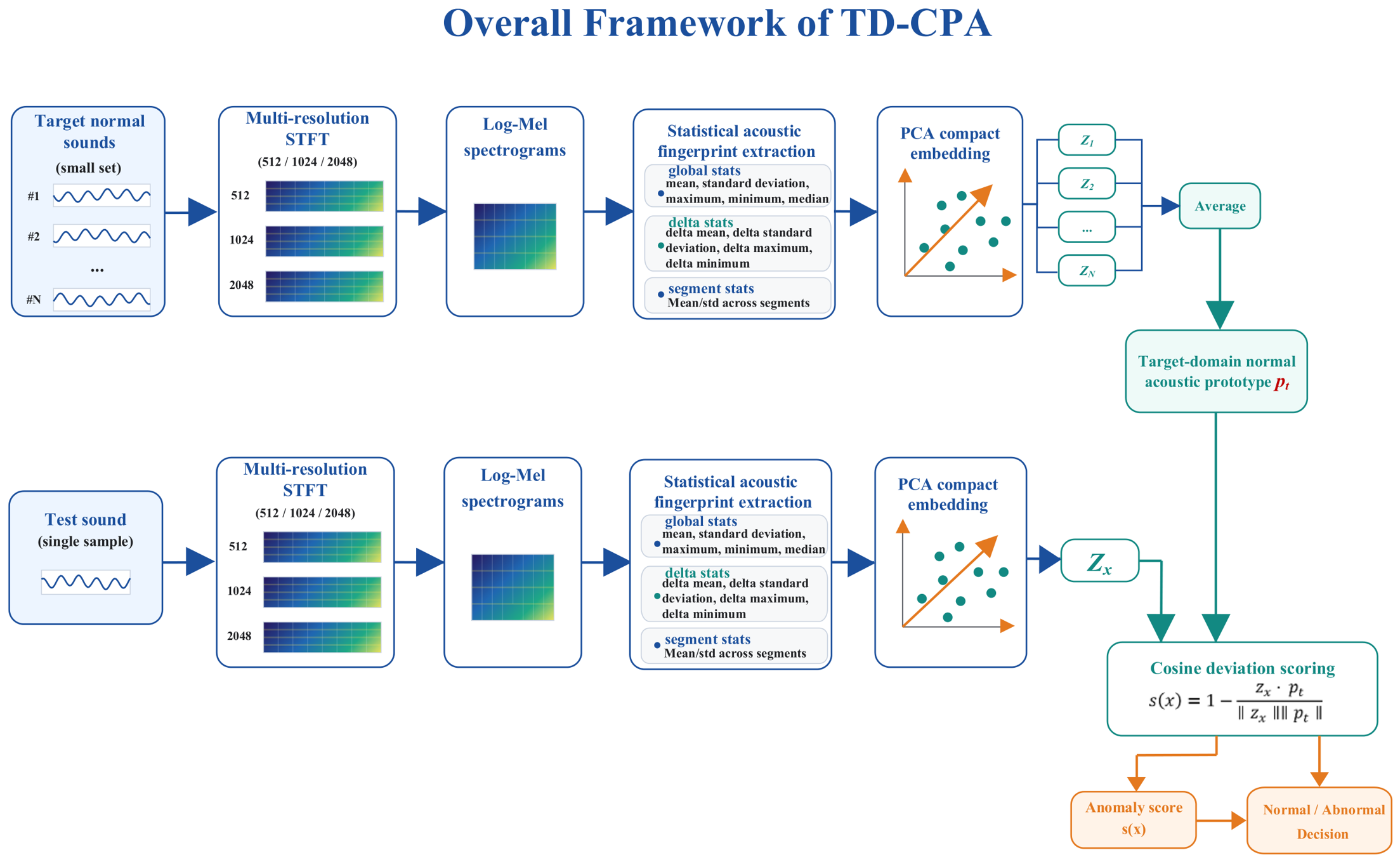
The proposed framework, referred to as target-domain cosine prototype anchoring (TD-CPA), combines multi-resolution acoustic fingerprints with target-normal prototype construction and cosine deviation scoring. It is designed for limited-sample industrial ASD, where only a small number of normal recordings from a target machine may be available, and representative anomalous recordings are difficult to obtain in advance. The framework separates normal-reference construction from test-time scoring and does not use anomaly labels during model construction.

As shown in Figure 1, the proposed method consists of two stages: target-normal prototype construction and test anomaly scoring. In the first stage, the normal training recordings are converted into multi-resolution Log-Mel spectrograms. Global band-wise, temporal-delta, segment-wise, Mel-band energy-ratio, and energy-envelope statistics are then concatenated into a 10,011-dimensional acoustic fingerprint. A PCA mapping fitted only from the normal training partition produces a compact embedding, and the 10 target-normal embeddings are averaged to form the target prototype. In the second stage, every test recording is transformed with the stored training parameters and scored by its cosine deviation from this fixed prototype. No test recording is used during PCA fitting or prototype construction.

The high-dimensional acoustic fingerprints are then projected into a compact embedding space using PCA to reduce redundancy and improve the stability of distance-based anomaly measurement [35,36]. The embeddings of target-normal samples are averaged to construct the target acoustic prototype, which represents the normal acoustic state of the monitored equipment.

In the testing stage, each sample is processed using the same feature-extraction and embedding procedure. The cosine deviation between the test embedding and the target prototype is used as the anomaly score. A larger deviation indicates a higher probability of an abnormal acoustic event. Overall, the method provides a simple and interpretable score for limited-sample industrial ASD under domain-shifted conditions. It may be extended to power equipment monitoring only after validation using field acoustic data.

2.2. Multi-Resolution Acoustic Fingerprint Representation

Industrial machine sounds may contain both stable operating components and short-duration abnormal variations. Stable components can arise from continuous rotation, mechanical vibration, fan operation, or background noise, while abnormal acoustic events may affect only short intervals or specific frequency bands. Log-Mel representations are widely used in ASD because they provide a compact description of time-varying spectral energy [1,24]. However, a single time-frequency resolution may not fully capture both transient changes and stable spectral patterns. Multi-resolution acoustic analysis is therefore used to retain complementary temporal and spectral information [2,25]. This rationale is general to industrial acoustic monitoring and does not imply that the evaluated anomalies are partial-discharge events.

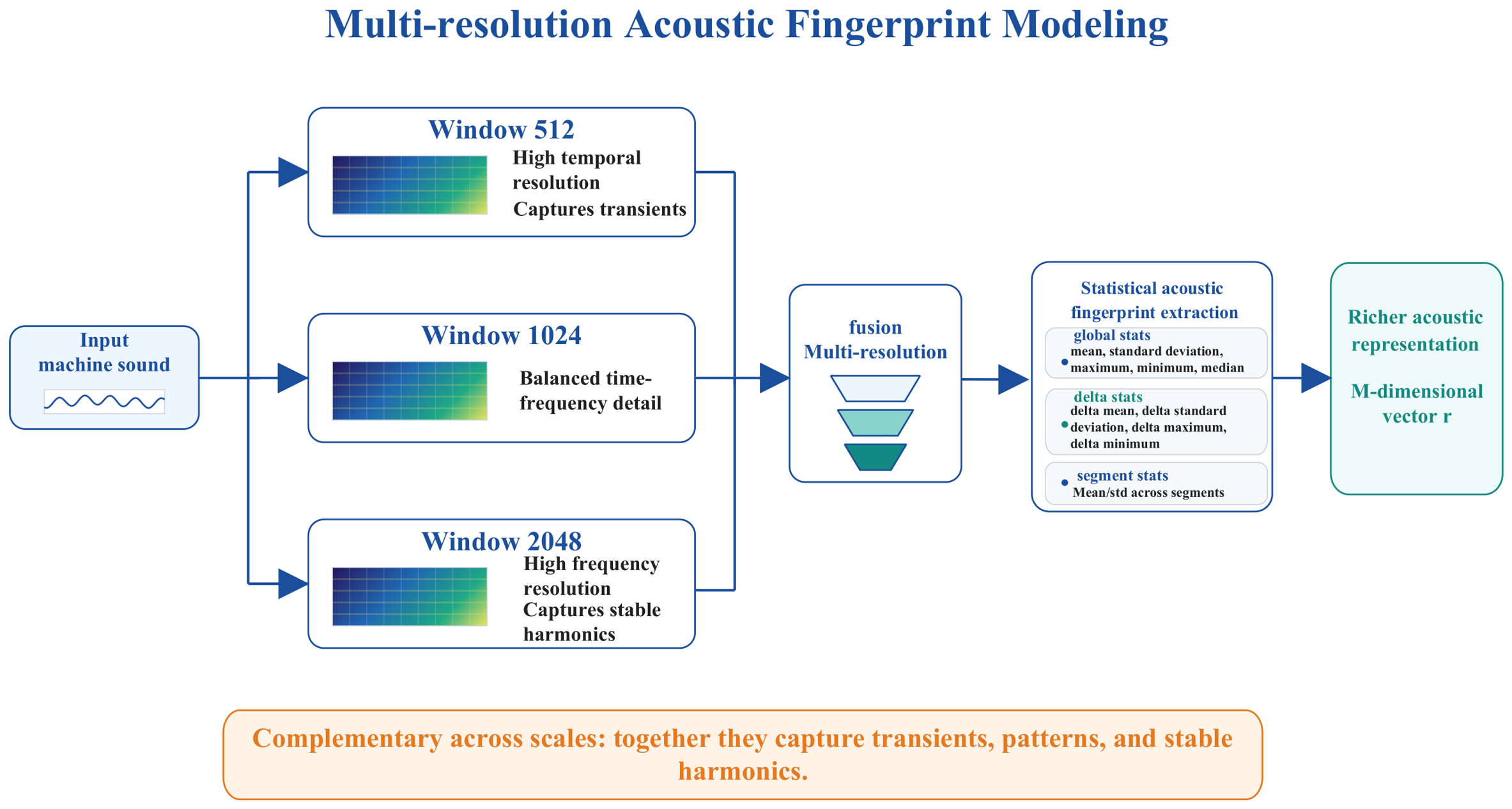
Abnormal acoustic events can affect different time scales. Short impacts, intermittent contacts, and rapid energy releases may be localized in time, while friction, looseness, and operating-state changes can modify longer spectral patterns [25,30]. In this study, multi-resolution means that the same 16 kHz waveform is processed in three parallel STFT branches with 512-, 1024-, and 2048-sample Hamming windows (32, 64, and 128 ms) and 50% overlap. The short window emphasizes timing, the long window emphasizes frequency structure, and the middle window provides an intermediate view. Each power spectrum is mapped to the same 128 Mel bands from 20 Hz to 8 kHz before statistical aggregation. Thus, the branches differ in analysis scale, not in the recordings used or the number of Mel bands. The complete acoustic-fingerprint extraction procedure is illustrated in Figure 2.

For an input acoustic waveform $x\left(n\right)$, this study constructs Log-Mel spectrograms under multiple time-frequency resolutions. The window length set is defined as:

$$\mathcal{N}=\left\{512, 1024, 2048\right\}$$

(1)

Different window lengths correspond to different time-frequency analysis scales. A shorter window provides higher temporal resolution and is more sensitive to transient acoustic changes, while a longer window provides higher frequency resolution and is more suitable for describing stable spectral structures. The medium window provides a balance between temporal and spectral resolution.

For the $r$-th resolution, the short-time Fourier transform (STFT) of the input signal is calculated as:

$$X_r\left(t,k\right)={\displaystyle \sum _{n=0}^{N_r-1}} x\left(n+tH\right)w_r\left(n\right)\exp \left(-j{\displaystyle \frac{2\pi kn}{N_r}}\right)$$

(2)

where $N_r$ is the window length of the $r$-th resolution, $H$ is the hop length, $w_r\left(n\right)$ is the window function, $t$ is the frame index, and $k$ is the frequency-bin index. The STFT converts the one-dimensional waveform into a time-frequency representation, which describes the variation in spectral energy over time.

The power spectrum is then projected onto the Mel filter bank and converted into a logarithmic scale. The Log-Mel spectrogram at the $r$-th resolution is calculated as:

$$M_r\left(t,m\right)=\log \left(ϵ+\sum _k B_{r,m}{\left|X_r(t,k)\right|}^2\right)$$

(3)

where $ϵ\in \{\mathrm{1,2},3\}$ denotes the resolution branch; $t\in \{1,\dots ,T_r\}$ is the time-frame index; $m\in \{1,\dots ,128\}$ is the Mel-band index; and $k=0,\dots ,F_r-1$ is the frequency-bin index. Here, $T_r$ and $F_r$ denote the numbers of time frames and nonnegative frequency bins at resolution $r$, respectively. $X_r(t,k)$ is the complex STFT coefficient at time frame $t$ and frequency bin $k$, and ${\left|X_r(t,k)\right|}^2$ is the corresponding power-spectrum value. $B_{r,m}\left(k\right)$ denotes the weight assigned to frequency bin $k$ by the $m$-th Mel filter at resolution $r$. The constant $\epsilon >0$ is introduced to ensure numerical stability and avoid taking the logarithm of zero.

The resulting Log-Mel spectrogram provides a compact time-frequency description of acoustic spectral energy and has been widely used in anomalous sound detection [24]. Because a single time-frequency resolution may not preserve both short-duration variations and relatively stable spectral structures, three complementary resolutions are used in this study. This design is also consistent with recent studies showing that frequency-aware and complementary spectral information can improve anomalous sound characterization [2,25].

Explicit statistical features are then extracted from each resolution to construct the acoustic fingerprint. This approach summarizes the principal temporal and spectral characteristics of the recordings without requiring end-to-end deep-network training, making it suitable for limited normal-sample conditions.

The fingerprint extraction process contains five components. First, global per-band statistics are calculated from both the original and per-band normalized Log-Mel spectrograms. Second, the mean, standard deviation, maximum, and minimum of the first-order temporal difference are calculated for each Mel band. Third, every spectrogram is divided into three approximately equal temporal segments, and the mean and standard deviation of the original and normalized values are calculated within each segment. Fourth, the relative energy of each Mel band is retained. Finally, nine statistics are used to summarize the frame-wise energy envelope and its first-order difference. The five feature groups contain 1152, 512, 1536, 128, and 9 values, respectively. Specifically, the global band-wise statistics contain 9 descriptors for each of the 128 Mel bands, producing 9 × 128 = 1152 values. The temporal-delta statistics contain 4 descriptors for each Mel band, producing 4 × 128 = 512 values. The segment-wise statistics contain the mean and standard deviation of both the raw and normalized Log-Mel spectrograms within K = 3 temporal segments, producing 2 × 2 × 3 × 128 = 1536 values. The Mel-band energy ratios contribute 128 values, while the energy-envelope statistics contribute 9 values. Therefore, each resolution produces 1152 + 512 + 1536 + 128 + 9 = 3337 values. Concatenating the three resolution branches results in a 10,011-dimensional acoustic fingerprint before PCA. Mel-band energy ratios and energy-envelope statistics are retained as common auxiliary features in all feature-component ablation settings.

The temporal delta features are extracted from the first-order temporal difference in the Log-Mel spectrogram:

$$D_r\left(t,m\right)=M_r\left(t,m\right)-M_r\left(t-1,m\right)$$

(4)

where $D_r\left(t,m\right)$ denotes the temporal change in the Log-Mel energy at frame $t$ and Mel band $m$. Compared with the original Log-Mel spectrogram, the delta representation emphasizes frame-to-frame acoustic variation. This is useful for describing sudden changes caused by transient abnormal events, especially when the abnormal information appears only in a short time interval.

The segment-wise statistical features are used to preserve coarse local temporal information. In practical acoustic monitoring, abnormal changes may occur only in part of a signal. If only global statistics are used, these local changes may be averaged out. Therefore, each Log-Mel spectrogram is divided into $K$ temporal segments, and statistical descriptors are calculated within each segment. In this study, $K$ = 3 is used. The segment-wise features can retain local acoustic differences while avoiding the high dimensionality of frame-level spectrogram modeling. The extracted acoustic fingerprint features are summarized in

Table 1. Feature components.

Feature Group	Input	Function
Global band-wise statistics	Raw and per-band normalized Log-Mel	Describe stable spectral distribution
Temporal-delta statistics	First difference in normalized Log-Mel	Capture frame-to-frame variation
Segment-wise statistics	Raw and normalized Log-Mel in K = 3 segments	Retain coarse local temporal structure
Mel-band energy ratios	Mean linear-scale Mel energy	Describe relative band-energy allocation
Energy-envelope statistics	Frame-wise mean Log-Mel and its first difference	Summarize overall energy and transient change
Multi-resolution concatenation	Features from 512/1024/2048-sample windows	Combine short-, medium-, and long-scale information

.

For each STFT resolution, the acoustic fingerprint is formed by concatenating five feature groups:

$$f_r=[f_r^G,f_r^D,f_r^S,f_r^B,f_r^E]$$

(5)

Here, $f_r$ denotes the acoustic fingerprint extracted using an $r$-sample STFT window. The five terms in Equation (5) represent the global band-wise, temporal-delta, segment-wise, Mel-band energy-ratio, and energy-envelope feature groups, respectively. The complete multi-resolution fingerprint is obtained as:

$$f=\left[f_{512},f_{1024},f_{2048}\right]$$

(6)

Here, $f$ denotes the final multi-resolution feature vector. Each resolution contributes 3337 values, resulting in a 10,011-dimensional fingerprint for each recording. The three STFT windows provide complementary time-frequency views, while the five statistical groups describe the overall spectral distribution, frame-to-frame variation, coarse local temporal structure, relative band-energy allocation, and frame-wise energy transients. The same feature-extraction procedure is applied to both normal training and test recordings, whereas PCA is fitted using only the normal training fingerprints and then applied unchanged to the test data.

2.3. Compact Embedding and Target Prototype Anchoring

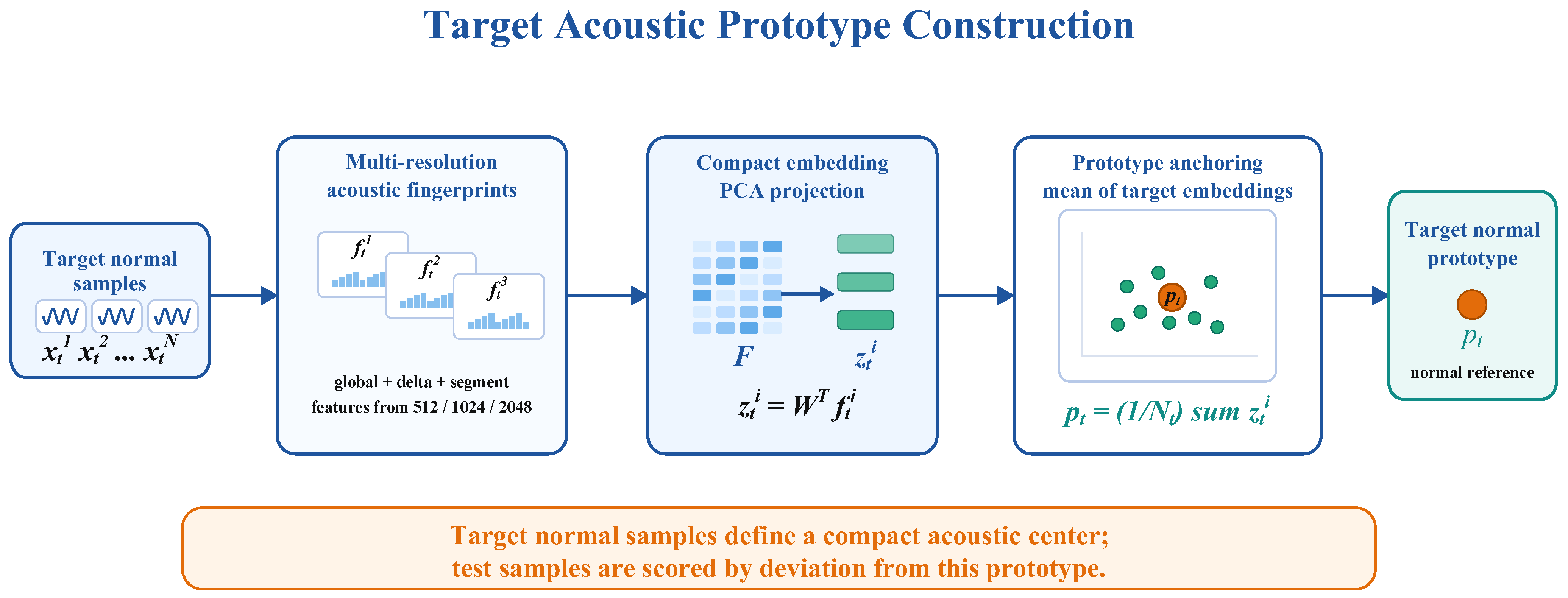
After multi-resolution acoustic fingerprint extraction, each acoustic sample is represented by a high-dimensional feature vector. Although the feature vector contains complementary information from different time-frequency resolutions, it may also include redundant and correlated components. Directly performing anomaly scoring in the original feature space may lead to unstable results, especially when only a limited number of target-normal samples are available. Therefore, this study first maps the multi-resolution acoustic fingerprint into a compact embedding space and then constructs a target acoustic prototype for normal-state modeling. The target prototype construction process is illustrated in Figure 3.

For each recording, the multi-resolution procedure produces a 10,011-dimensional acoustic fingerprint. Per-band normalization is performed within each spectrogram branch when the normalized statistical features are calculated. No target-only normalization is applied to the final fingerprints.

For each machine section, the fingerprints of all 1000 normal training recordings, including 990 source-normal and 10 target-normal recordings, are arranged as the training matrix $X_{\mathrm{train}}$. The training matrix is centered using its column-wise mean:

$$X_c=X_{\mathrm{train}}-1{{\mu }_{\mathrm{PCA}}}^T,{\mu }_{\mathrm{PCA}}={\displaystyle \frac{1}{1000}}{\displaystyle \sum _{i=1}^{1000}}{f}_i$$

(7)

Here, $f_i$ is the 10,011-dimensional fingerprint of the $i$-th normal training recording, ${\mu }_{\mathrm{PCA}}$ is the column-wise mean of the training fingerprints, 1 is a 1000-dimensional vector of ones, and $X_c$ is the centered training matrix. Both $X_{\mathrm{train}}$ and $X_c$ contain 1000 rows and 10,011 columns. No test recording is used to calculate ${\mu }_{\mathrm{PCA}}$ or construct $X_c$.

PCA is fitted separately for each evaluated machine section using the complete normal training partition rather than only the 10 target-normal recordings. Singular value decomposition is applied to $X_c$, and the 128 right singular vectors associated with the largest singular values form the projection matrix $W$. Because the centered training matrix has a maximum rank of 999, retaining 128 principal components is mathematically feasible. The rank-at-most-nine restriction would apply only if PCA were fitted using the 10 target-normal recordings alone, which is not the procedure adopted in this study.

Each fingerprint is projected and standardized as follows:

$$q_i=W^T(f_i-{\mu }_{\mathrm{PCA}}),z_i={\displaystyle \frac{q_i-{\mu }_z}{{\sigma }_z}}$$

(8)

Here, $W$ is the PCA projection matrix, $q_i$ is the 128-dimensional PCA coordinate vector of the $i$-th recording, and $z_i$ is its standardized compact embedding. The vectors ${\mu }_z$ and ${\sigma }_z$ denote the coordinate-wise mean and standard deviation calculated from the PCA coordinates of the same 1000 normal training recordings. The division in Equation (8) is performed element by element. A small positive constant is included in ${\sigma }_z$ during implementation to ensure numerical stability. The centering vector, projection matrix, and coordinate-standardization parameters are stored and applied unchanged to all subsequent recordings. Thus, every recording is represented in the same normal-training-derived embedding space, while target-domain information is introduced through the target prototype.

After obtaining the compact embeddings, the target-normal embedding set is defined as:

$$D_t^n=\left\{z_1^t,z_2^t,\dots ,z_{N_t}^t\right\}$$

(9)

Here, $D_t^n$ denotes the target-normal embedding set, $N_t$ is the number of available target-normal recordings, and $z_i^t$ is the compact embedding of the $i$-th target-normal recording. The superscript $t$ indicates the target domain, while the superscript $n$ denotes normal data. The target-normal prototype is calculated by averaging all target-normal embeddings:

$$p_t={\displaystyle \frac{1}{N_t}}{\displaystyle \sum _{i=1}^{N_t}} z_i^t$$

(10)

Here, $p_t$ denotes the target-normal acoustic prototype. In the main experiment, $N_t=10$, so the prototype is the arithmetic mean of the 10 target-normal embeddings in the fixed 128-dimensional space. It serves as an algebraic target-domain reference rather than a learned classifier. No test or anomalous recording is used for PCA fitting, coordinate standardization, or prototype construction, and the prototype remains fixed throughout the reported evaluation.

Prototype-based similarity scoring has previously been investigated in ASD [15,16]. Therefore, prototype averaging and cosine scoring are not presented as standalone innovations. The contribution of this study lies in integrating target-normal prototype anchoring with the proposed multi-resolution statistical fingerprint and compact PCA embedding.

This construction is suitable for limited-sample industrial ASD, where only a few normal recordings may be available from a newly deployed target machine and representative anomalous recordings are difficult to obtain. This setting is consistent with first-shot and few-shot ASD studies that focus on adaptation to new target machines using limited target-domain data [16,21,37]. The target prototype provides a compact representation of the normal acoustic state and serves as the reference for subsequent anomaly scoring. Test recordings close to the prototype are considered more consistent with the target-normal state, while larger deviations indicate a higher likelihood of abnormal acoustic behavior. The main variables used in the proposed method are summarized in

Table 2. Main variables for compact embedding and prototype construction.

Symbol	Description
fi	10,011-dimensional multi-resolution fingerprint of the i-th recording
Xtrain	1000 × 10,011 normal-training fingerprint matrix (990 source and 10 target recordings)
μPCA	Column mean of the normal-training matrix used to center every training and test fingerprint
W	10,011 × 128 PCA projection matrix fitted from the centered normal-training matrix
qi	Unstandardized 128-dimensional PCA coordinate of the i-th recording
zi	128-dimensional embedding standardized with normal-training projected-coordinate statistics
Nt	Number of target-normal recordings used to construct the prototype
pt	Arithmetic mean of the target-normal embeddings

.

2.4. Cosine Deviation-Based Anomaly Scoring

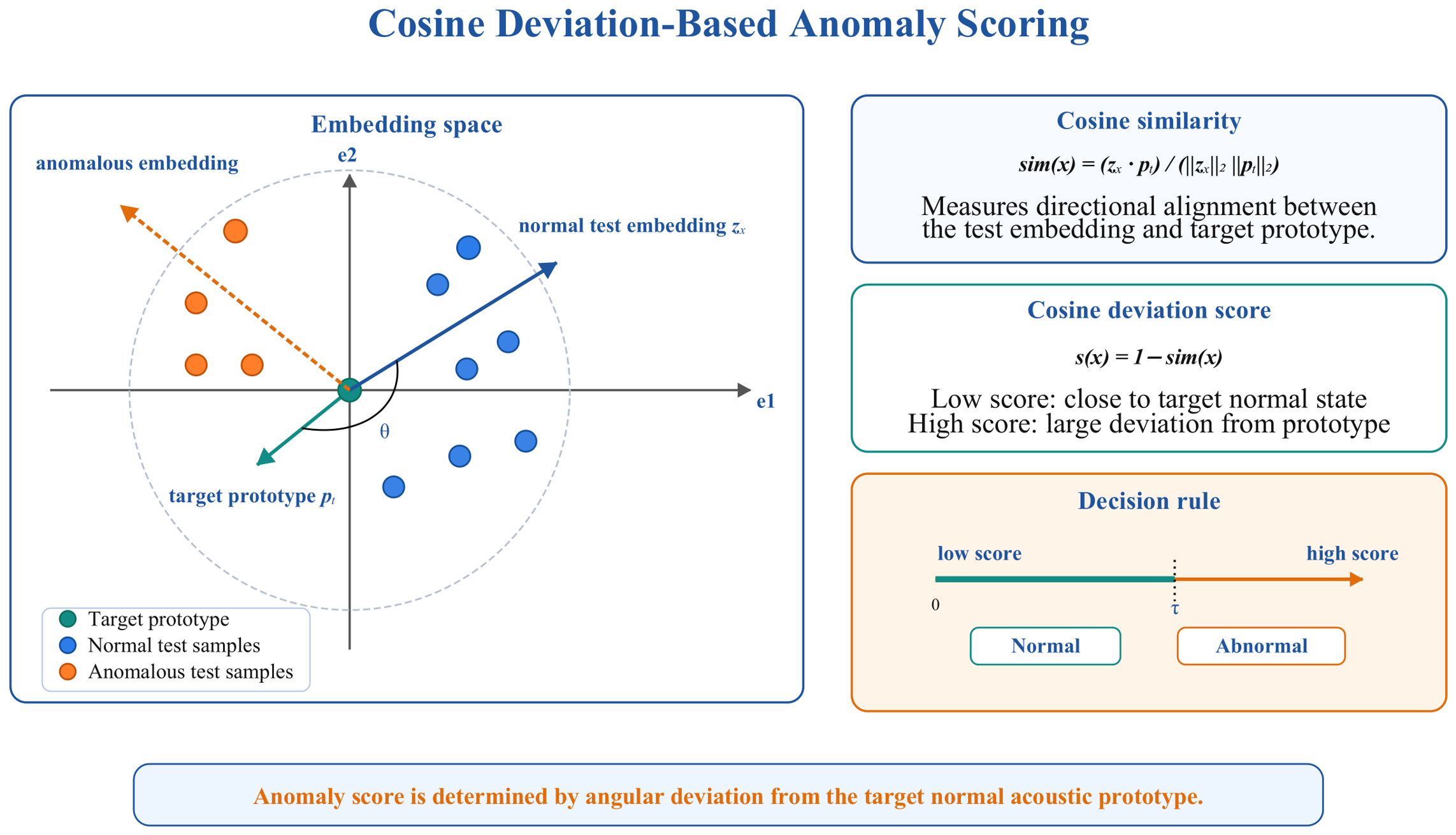
After constructing the target-normal acoustic prototype, anomaly detection measures the deviation between each test sample and the prototype in the compact embedding space. Because model construction uses normal recordings only, anomalous recordings are not required in advance. This setting reflects industrial monitoring situations in which representative fault data are rare or unavailable. The test-time cosine deviation scoring process is shown in Figure 4.

For each test recording $x$, the 10,011-dimensional fingerprint $f_x$ is extracted using the same multi-resolution procedure as that applied to the training recordings. The stored normal-training parameters are then used to obtain the compact test embedding

$$q_x=W^T(f_x-{\mu }_{\mathrm{PCA}}),z_x={\displaystyle \frac{q_x-{\mu }_z}{{\sigma }_z}}$$

(11)

Here, $f_x$ is the acoustic fingerprint of test recording $x$, $q_x$ is its 128-dimensional PCA coordinate vector, and $z_x$ is the corresponding standardized compact embedding. The projection matrix $W$, fingerprint-centering vector ${\mu }_{\mathrm{PCA}}$, and coordinate-standardization parameters ${\mu }_z$ and ${\sigma }_z$ are obtained from the 1000 normal training recordings, as described in Section 2.3. The division in Equation (11) is performed element by element. These parameters remain fixed and are not recalculated using the test recordings.

The similarity between the test embedding $z_x$ and the target-normal acoustic prototype $p_t$ is calculated using cosine similarity:

$$\mathrm{s}\mathrm{i}\mathrm{m}(x)={\displaystyle \frac{z_x^T{p}_t}{{∥z_x∥}_2{∥p_t∥}_2}}$$

(12)

Here, $\mathrm{s}\mathrm{i}\mathrm{m}\left(x\right)$ denotes the cosine similarity of test recording $x$, $p_t$ is the target-normal prototype defined in Equation (10), and ${∥·∥}_2$ denotes the Euclidean norm. Cosine similarity measures the directional consistency between two embedding vectors and is less sensitive than Euclidean distance to differences in their overall magnitudes. This property is useful in acoustic monitoring because variations in sensor position, propagation path, operating condition, and background noise may affect the magnitude of the extracted acoustic representation. Therefore, cosine similarity provides a direction-based comparison between the test embedding and the target-normal prototype while reducing sensitivity to uniform changes in embedding magnitude.

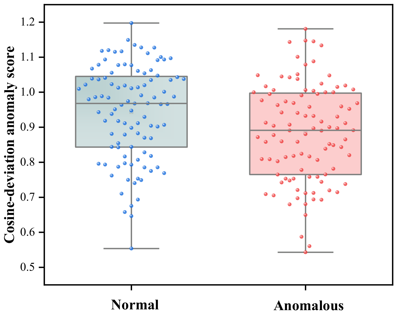
The anomaly score is defined as the cosine deviation from the target prototype:

$$s\left(x\right)=1-\mathrm{sim}\left(x\right)$$

(13)

A smaller value of $s\left(x\right)$ indicates that the test sample is close to the target-normal acoustic prototype, suggesting that the equipment sound is consistent with the normal operating state. Conversely, a larger value of $s\left(x\right)$ indicates that the test sample deviates from the target-normal acoustic pattern and is more likely to correspond to an abnormal acoustic event. In this way, the proposed method converts the similarity relationship between the test embedding and the target prototype into an interpretable anomaly score.

For practical decision-making, the anomaly score can be compared with a decision threshold:

$$\widehat{y}\left(x\right)=\left\{\begin{array}{c}0, s\left(x\right)<\tau \\ 1, s\left(x\right)\ge \tau \end{array}\right.$$

(14)

where $\tau$ is the decision threshold, $\widehat{y}\left(x\right)=0$ denotes a normal sample, and $\widehat{y}\left(x\right)=1$ denotes an abnormal sample. In field applications, the threshold can be determined according to the score distribution of normal validation samples or according to the required false alarm level. In the experimental evaluation of this study, threshold-independent metrics such as AUC and pAUC are also used to evaluate the ranking ability of the anomaly score without relying on a fixed threshold.

The cosine deviation-based scoring strategy is consistent with recent ASD studies that evaluate abnormality through prototype similarity or compact embedding comparison [37,38]. Compared with reconstruction-error-based methods, the proposed strategy does not require a decoder. Compared with classification-based methods, it does not require abnormal labels or many target samples. The anomaly score is directly obtained from the deviation between the test embedding and the target-normal prototype, making the process simple and interpretable.

For each test sample, the same feature extraction pipeline is used to generate the multi-resolution acoustic fingerprint. After normalization and PCA projection, the cosine deviation between the test embedding and the target-normal prototype is calculated as the anomaly score. This provides a direct measure of how much the test acoustic pattern deviates from the Target-normal acoustic state.

3. Data Source and Experimental Methodology

3.1. Data Source

The experiments used the public DCASE Challenge 2023 Task 2 development dataset for first-shot unsupervised anomalous sound detection [5,6,7]. Seven machine categories were evaluated: bearing, fan, gearbox, slider, ToyCar, ToyTrain, and valve.

The experiments used the official partition without additional subsampling. For every evaluated section, the training set contains 990 source-domain normal recordings and ten target-domain normal recordings, whereas the test set contains 100 normal and 100 anomalous recordings. All 1000 training files and all 200 test files were enumerated in the main experiment.

Only the ten target-domain normal training recordings were used to form the target prototype. The 990 source-domain normal recordings were retained for normalization, PCA construction, and source-based baseline comparisons, as specified for each method. Test recordings were never used for feature normalization, PCA fitting, prototype construction, model training, or hyperparameter selection.

Table 3. Dataset composition used in this study.

Machine Category	Normal Training Samples	Normal Test Samples	Anomalous Test Samples
Bearing	1000 (990 source + 10 target)	100	100
Fan	1000 (990 source + 10 target)	100	100
Gearbox	1000 (990 source + 10 target)	100	100
Slider	1000 (990 source + 10 target)	100	100
ToyCar	1000 (990 source + 10 target)	100	100
ToyTrain	1000 (990 source + 10 target)	100	100
Valve	1000 (990 source + 10 target)	100	100

reports the exact official composition of each evaluated section.

The seven evaluated sections cover real and toy machine acoustics with different operating and anomaly patterns. Results are calculated separately for each section and then averaged across the seven categories; no aggregation is performed across multiple sections within a category.

3.2. Target Acoustic Prototype Construction

The experiments followed a normal-only setting and retained the official data partition described above. For each machine section, PCA and projected-coordinate standardization were fitted once using all 1000 normal training recordings (990 source and ten target); test data were excluded. The ten target-normal embeddings were then averaged to form the target prototype. This separation avoids the rank deficiency of target-only PCA while keeping prototype construction target-specific. Anomalous test recordings were used solely for final evaluation.

All recordings were converted into single-channel waveforms and processed with the same fixed feature pipeline. Three Log-Mel spectrograms were computed with 512-, 1024-, and 2048-sample STFT windows and 128 Mel filters. At every resolution, global band-wise, temporal-delta, segment-wise, Mel-band energy-ratio, and energy-envelope statistics were extracted, giving 3337 values per branch and 10,011 values after concatenation. The segment number was K = 3. PCA and projected-coordinate standardization were then fitted only from the normal training partition.

PCA reduced the fingerprint dimension to 128. Each test recording was transformed using the training-fitted statistics and PCA projection, and its anomaly score was defined as one minus the cosine similarity to the target-normal prototype. For the N_t sensitivity experiment, only the number of target-normal embeddings used to form the prototype was changed; the feature normalization, PCA projection, test set, and score definition remained fixed. The complete experimental configuration is summarized in

Table 4. Experimental parameter settings.

Item	Setting
Evaluated machine sections	section_00 of bearing, fan, gearbox, slider, ToyCar, ToyTrain, and valve
Official training partition per section	990 source-normal + 10 target-normal recordings
Official test partition per section	100 normal + 100 anomalous recordings
Additional subsampling in main experiment	None
Target-normal samples for main prototype	10
STFT window lengths	512, 1024, and 2048 samples
Number of Mel filters	128
Temporal segments	3
Feature groups	Global, temporal-delta, segment-wise, Mel-band-ratio, and energy-envelope statistics
Dimensionality reduction	Training-fitted PCA, 128 dimensions
Prototype construction	Mean embedding of target-normal recordings
Scoring rule	1-cosine similarity
Evaluation metrics	AUC, normalized pAUC at FPR ≤ 0.1, and HScore

.

The above parameter settings were kept the same across all machine categories to ensure a fair comparison. No machine-specific parameter tuning was performed in the main experiment. This design was adopted to evaluate whether the proposed method can provide stable anomaly detection performance under a unified configuration. In addition, ablation experiments were conducted by changing the prototype source, distance metric, feature component, and resolution setting, so that the contribution of each key module could be further analyzed in Section 4.

3.3. Baseline Methods and Evaluation Metrics

The comparison includes statistical and distance-based baselines, a compact convolutional autoencoder (Conv-AE), and a frozen pretrained YAMNet embedding baseline. All methods used the same official training and test partitions, no anomalous recording was used for training or parameter selection, and all sample-level scores were evaluated with the same AUC, normalized pAUC (maximum FPR 0.1), and HScore implementation.

For prototype construction, source-prototype, all-training-sample prototype, and target-prototype methods were compared. This comparison was used to examine whether modeling the target equipment with its own normal samples can reduce source-target distribution mismatch.

For distance metrics, cosine deviation, Euclidean distance, and diagonal Mahala nobis distance were evaluated under the same target-prototype setting. This comparison was used to analyze how different distance measures affect anomaly scoring.

The compact Conv-AE used a 64 × 64 Log-Mel input, convolutional channels 8-16-32 with a symmetric transposed-convolution decoder, 15 epochs, batch size 64, and learning rate 0.001; it was trained separately for each machine using all 1000 normal training recordings, and mean reconstruction MSE was used as the score. The pretrained baseline used the frozen YAMNet global-average-pooling embedding (1024 dimensions), mean-pooled over patches, followed by the same ten-sample target prototype and cosine deviation backend [39]. These are transparent representative baselines rather than an exhaustive reproduction of every deep ASD system. The baseline configurations and their roles are summarized in

Table 5. Baseline methods used for comparison.

Method	Reference Data	Scoring Strategy	Purpose
Source prototype	990 source-normal	Cosine deviation	Source-domain reference
All-training prototype	All 1000 normal	Cosine deviation	Mixed-domain reference
Target prototype	10 target-normal	Cosine deviation	TD-CPA backend
Target kNN	10 target-normal	kNN cosine distance	Local target reference
Source kNN	Source-normal subset	kNN cosine distance	Local source reference
Source-target kNN fusion	Source- and target-normal	Fused kNN distance	Mixed local reference
PCA reconstruction	Normal training recordings	Reconstruction error	Linear reconstruction baseline
Target prototype + Euclidean	10 target-normal	Euclidean distance	Distance-metric comparison
Target prototype + Mahalanobis	10 target-normal	Diagonal Mahalanobis	Variance-weighted comparison
Compact Conv-AE	All 1000 normal per machine	Log-Mel reconstruction MSE	Autoencoder baseline
Frozen YAMNet + target prototype	Pretrained embedding + 10 target-normal	Cosine deviation	Pretrained-embedding baseline
TD-CPA	All normal for PCA; 10 target-normal for prototype	Cosine deviation	Proposed integrated framework

.

The anomaly detection performance was evaluated using AUC, pAUC, and HScore. AUC measures the overall ranking ability of anomaly scores across different decision thresholds. A higher AUC indicates that anomalous samples tend to receive higher anomaly scores than normal samples. It is calculated as:

$$\mathrm{A}\mathrm{U}\mathrm{C}={\int }_0^1\mathrm{T}\mathrm{P}\mathrm{R}\left(\mathrm{F}\mathrm{P}\mathrm{R}\right)d\mathrm{F}\mathrm{P}\mathrm{R}$$

(15)

where TPR and FPR denote the true positive rate and false positive rate, respectively.

In practical condition monitoring systems, the low-false-alarm region is particularly important because excessive false alarms may reduce the reliability and usability of online monitoring. Therefore, pAUC was also used to evaluate the detection performance under a limited false-positive-rate range. In this study, pAUC is defined as:

$$\mathrm{p}\mathrm{A}\mathrm{U}\mathrm{C}={\displaystyle \frac{1}{\alpha }}{\int }_0^{\alpha }\mathrm{T}\mathrm{P}\mathrm{R}\left(\mathrm{F}\mathrm{P}\mathrm{R}\right)d\mathrm{F}\mathrm{P}\mathrm{R}$$

(16)

where $\alpha$ denotes the maximum false positive rate considered in the partial AUC calculation. This metric focuses on the ranking performance of anomaly scores in the low-FPR region and is commonly used in anomalous sound detection benchmarks such as DCASE Task 2 [8].

To jointly consider the overall detection ability and low-false-alarm performance, HScore was used as a combined indicator of AUC and pAUC. It is calculated as the harmonic mean of AUC and pAUC:

$$\mathrm{H}\mathrm{S}\mathrm{c}\mathrm{o}\mathrm{r}\mathrm{e}={\displaystyle \frac{2\cdot \mathrm{A}\mathrm{U}\mathrm{C}\cdot \mathrm{p}\mathrm{A}\mathrm{U}\mathrm{C}}{\mathrm{A}\mathrm{U}\mathrm{C}+\mathrm{p}\mathrm{A}\mathrm{U}\mathrm{C}}}$$

(17)

A higher HScore indicates a better balance between global ranking and low-FPR performance. The same AUC, normalized pAUC, and HScore implementations were used for the main method, all baselines, the machine-wise analysis, the ablation study, and the newly added experiments. Metrics were calculated separately for each machine section and then averaged across the seven sections.

In addition to the overall comparison, ablation experiments were conducted to further analyze the contribution of each component in the proposed method. Specifically, the effects of prototype source, distance metric, feature component, and multi-resolution modeling were evaluated separately. These experiments were designed to answer four questions: whether target prototype anchoring is more effective than source or mixed prototypes, whether cosine deviation is more suitable than Euclidean or Mahalanobis distance, whether global, delta, and segment-wise features are complementary, and whether multi-resolution modeling improves performance compared with a single-resolution representation. These analyses are presented in Section 4.

4. Results and Discussion

4.1. Overall Detection Performance and Metric Analysis

Table 6. Overall performance comparison of different methods.

Method	Mean AUC	Mean pAUC	Mean HScore
TD-CPA: target prototype + cosine	0.6067	0.1389	0.2095
Source-target kNN fusion + cosine	0.5849	0.1171	0.1907
Target-kNN + cosine	0.5627	0.1178	0.1821
Target prototype + Euclidean	0.5821	0.0806	0.1381
Target prototype + DiagMahalanobis (train)	0.5821	0.0806	0.1381
Target prototype + DiagMahalanobis (target-reg)	0.5785	0.0737	0.1279
Source-kNN + cosine	0.5636	0.0731	0.1262
PCA reconstruction using target train	0.5830	0.0699	0.1211
PCA reconstruction using all train	0.6017	0.0656	0.1161
Frozen YAMNet + target prototype	0.5747	0.0666	0.1135
Compact Conv-AE	0.4833	0.0569	0.1003
All-training prototype + cosine	0.4981	0.0495	0.0887
Source prototype + cosine	0.3837	0.0348	0.0623

reports the results under the evaluation convention used throughout the experiments. TD-CPA achieved the highest numerical mean values among the evaluated methods: AUC 0.6067, pAUC 0.1389, and HScore 0.2095. Source-target kNN fusion obtained the next-highest HScore (0.1907). The added frozen YAMNet and compact Conv-AE baselines achieved mean HScore values of 0.1135 and 0.1003, respectively.

As shown in Table 6 and Figure 5, TD-CPA achieved the highest numerical mean HScore among the evaluated methods, exceeding source-target kNN fusion by 0.0188. This result demonstrates the competitive overall performance of TD-CPA under the current experimental setting. The statistical reliability of this difference is further examined through the paired bootstrap analysis in Section 4.4, whereas the machine-wise results and confidence intervals provide additional insight into its performance across different categories.

PCA reconstruction using all normal training recordings achieved a mean AUC of 0.6017, close to TD-CPA’s 0.6067, but its mean pAUC and HScore were lower (0.0656 and 0.1161). The added deep baselines also showed machine-dependent behavior: frozen YAMNet achieved a mean HScore of 0.1135 and the compact Conv-AE achieved 0.1003, neither surpassing TD-CPA under this shared normal-only protocol. These results support describing TD-CPA as competitive and lightweight, rather than claiming universal superiority over modern ASD models.

The source and all-training prototypes produced mean HScore values of 0.0623 and 0.0887, respectively, whereas the target prototype with cosine scoring produced 0.2095. This numerical comparison indicates that the target-normal reference is useful under the evaluated domain shift, although it does not establish that one prototype is sufficient for every machine category.

The machine-wise results in

Table 7. Machine-wise performance of the proposed method.

Machine Category	AUC	pAUC	HScore
Bearing	0.6581	0.1575	0.2542
Fan	0.4680	0.0145	0.0281
Gearbox	0.6272	0.0630	0.1145
Slider	0.8584	0.4205	0.5645
ToyCar	0.4760	0.0330	0.0617
ToyTrain	0.3668	0.0375	0.0680
Valve	0.7922	0.2460	0.3754

show the strongest AUC values for slider (0.8584) and valve (0.7922). Bearing and gearbox were intermediate, whereas fan, ToyCar, and ToyTrain remained difficult. In particular, ToyTrain retained an AUC below 0.5 and is examined separately in Section 4.3.

The results in Table 7 and Figure 6 show that slide and valve achieved relatively strong detection performance, indicating that their normal and anomalous acoustic patterns can be effectively separated by the proposed multi-resolution acoustic fingerprint and target-prototype scoring strategy. For these categories, anomalous samples produced larger cosine deviations from the target-normal prototype.

In contrast, fan, ToyCar, and ToyTrain were more challenging in the low-FPR region. In particular, the AUC below 0.5 for ToyTrain indicates that anomalous recordings tended to receive lower scores than normal recordings under the current representation. A detailed sample-level analysis of this behavior is presented in Section 4.3.

Overall, TD-CPA achieved the highest numerical mean performance among the evaluated methods, demonstrating its competitiveness under the current experimental protocol. Performance differences across machine categories and the paired bootstrap results are further analyzed to provide a more complete assessment of the method’s effectiveness and statistical reliability.

4.2. Comparative Analysis of Prototype and Scoring Strategies

Table 8. Comparison of prototype construction and scoring strategies.

Method	Reference Data	Scoring Strategy	Mean AUC	Mean pAUC	Mean HScore
TD-CPA: Target-prototype + cosine	Target-normal samples	Cosine deviation	0.6067	0.1389	0.2095
Source-target kNN fusion + cosine	Source and target-normal samples	kNN fusion distance	0.5849	0.1171	0.1907
Target-kNN + cosine	Target-normal samples	kNN distance	0.5627	0.1178	0.1821
Source-kNN + cosine	Source normal samples	kNN distance	0.5636	0.0731	0.1262
All-train-prototype + cosine	All normal training samples	Cosine deviation	0.4981	0.0495	0.0887
Source-prototype + cosine	Source normal samples	Cosine deviation	0.3837	0.0348	0.0623
Target-prototype + Euclidean	Target-normal samples	Euclidean distance	0.5821	0.0806	0.1381
Target-prototype + DiagMahalanobis (train)	Target-normal samples	Diagonal Mahalanobis distance	0.5821	0.0806	0.1381
Target-prototype + DiagMahalanobis (target-reg)	Target-normal samples	Diagonal Mahalanobis distance	0.5785	0.0737	0.1279

compares different normal-reference sources and scoring metrics under the same evaluation protocol. Among the evaluated configurations, the target-prototype cosine strategy achieved the highest mean performance, indicating that a target-aligned normal reference and a direction-based similarity measure work effectively with the proposed acoustic representation. As prototype construction and cosine scoring have previously been investigated in ASD [15,16], the contribution of TD-CPA lies in their integration with the multi-resolution statistical fingerprint rather than in either component individually.

The target-prototype cosine configuration increased the numerical mean HScore from 0.0623 for the source prototype and 0.0887 for the all-training prototype to 0.2095. This suggests that a target-aligned reference can reduce the effect of source-target mismatch in the evaluated sections, but the ToyTrain result shows that a single target prototype can still be inadequate when the target-normal distribution is poorly covered or multimodal.

The corresponding effects of prototype source and scoring distance are visualized in Figure 7.

Using ten target-normal recordings gave a more representative reference than the source-only and mixed-domain means on average. This observation is restricted to the present data partition; the sensitivity analysis in Section 4.4 shows that performance and variability depend on N_t and on which target-normal recordings are selected.

The kNN methods were competitive: source-target kNN fusion reached a mean HScore of 0.1907, close to TD-CPA’s 0.2095. The paired bootstrap interval for their HScore difference includes zero, so the comparison does not support a statistically significant superiority claim.

Under the same target-prototype setting, cosine deviation achieved the highest numerical mean HScore of 0.2095, compared with 0.1381 for Euclidean distance, 0.1381 for diagonal Mahalanobis distance using normal-training variance estimates, and 0.1279 for target-regularized diagonal Mahalanobis distance. These results suggest that cosine deviation is better suited to the current normalized embedding space, possibly because it emphasizes directional consistency while reducing sensitivity to variations in embedding magnitude. Nevertheless, this observation is specific to the proposed acoustic fingerprint, embedding procedure, and evaluated dataset, and should not be interpreted as a general advantage of cosine distance in all ASD tasks.

Taken together, the results show that the proposed multi-resolution fingerprint, target-normal anchoring, and cosine scoring form a competitive lightweight combination. They do not establish prototype cosine scoring as a new method on its own, nor do they rule out stronger performance from alternative learned embeddings or multi-prototype representations.

4.3. ToyTrain Failure-Case Diagnosis

A sample-level audit was conducted because ToyTrain’s AUC was below 0.5. The labels matched the normal/anomaly filenames; anomalous recordings were the positive ROC class; the anomaly score was exactly 1-cosine similarity; the prototype used only the ten target-normal training recordings; no test or anomalous recording entered the prototype; and PCA was fitted only on normal training features. Recomputing the stored scores from the cached fingerprints changed them by at most 4.88 × 10⁻¹⁵. Thus, the low AUC is not caused by a sign error, label reversal, test leakage, or prototype contamination.

Under the unchanged evaluation convention used for all formal results, ToyTrain obtained AUC 0.3668, pAUC 0.0375, and HScore 0.0680. Reversing the scores produced a diagnostic AUC of 0.6233, confirming inverted ranking, but the reversed score was not used in any formal result. Normal test recordings had a mean anomaly score of 0.9435 (median 0.9680, standard deviation 0.1350, range 0.5537–1.1976), while anomalous recordings had a lower mean of 0.8832 (median 0.8912, standard deviation 0.1395, range 0.5430–1.1810). The target-normal training recordings had a mean distance of 0.6349 to their prototype. Therefore, the anomalies were, on average, closer to the prototype than the normal test recordings. A plausible failure mode is that one mean prototype built from ten recordings does not cover ToyTrain’s multimodal normal variability, leading to overlap and structural misalignment in the current embedding. As shown in Figure 8, the anomalous-score distribution overlaps substantially with the normal-score distribution and is shifted slightly downward, which is consistent with the inverted ranking observed for ToyTrain.

4.4. Statistical Comparison and Target-Sample Sensitivity

Paired stratified bootstrap tests were performed on sample-level scores with 10,000 replicates. Within every machine section, normal and anomalous recordings were resampled separately with replacement, and identical indices were used for the two compared methods. The mean AUC difference between TD-CPA and PCA reconstruction using all training recordings was 0.0049 (95% CI −0.0389 to 0.0489, p = 0.8288). Against source-target kNN fusion, the mean pAUC difference was 0.0217 (95% CI −0.0149 to 0.0617, p = 0.2368) and the mean HScore difference was 0.0188 (95% CI −0.0283 to 0.0689, p = 0.4038). None of these differences were significant at p < 0.05;

Table 9. Paired bootstrap comparisons between TD-CPA and the strongest baseline methods.

Comparison	Metric	Difference	95% CI	p-Value	Significant
TD-CPA vs. PCA-All	Mean AUC	0.0049	[−0.0389, 0.0489]	0.8288	No
TD-CPA vs. ST-kNN	Mean pAUC	0.0217	[−0.0149, 0.0617]	0.2368	No
TD-CPA vs. ST-kNN	Mean HScore	0.0188	[−0.0283, 0.0689]	0.4038	No

therefore supports the wording “highest numerical mean” rather than “significantly outperformed.”

Sensitivity to the number of target-normal recordings was evaluated for N_t in {1, 2, 3, 5, 7, 10}. For N_t < 10, recordings were sampled without replacement from the same 10 target-normal recordings over 30 repetitions with fixed seeds; only prototype membership changed. Mean AUC increased from 0.5448 ± 0.0246 at N_t = 1 to 0.5957 ± 0.0133 at N_t = 7 and 0.6067 at N_t = 10. Mean HScore increased from 0.1349 ± 0.0259 to 0.1997 ± 0.0231 and 0.2095, respectively. The trend supports an average benefit from additional target-normal coverage, whereas the larger variation at very small N_t shows sensitivity to sample selection. Consequently, the few-sample claim is limited to the tested range and does not imply that ten recordings always represent a complex normal distribution. The performance trends and standard deviations across the evaluated N_t values are shown in Figure 9.

4.5. Ablation Analysis and Practical Discussion

As shown in

Table 10. Ablation results of feature components and resolution settings.

Ablation Type	Setting	Mean AUC	Mean pAUC	Mean HScore
Feature component	Full features	0.6067	0.1389	0.2095
Feature component	Global + delta features	0.6021	0.1369	0.2056
Feature component	Global features	0.5954	0.1014	0.1654
Feature component	Global + segment features	0.5923	0.0940	0.1530
Resolution setting	512 + 1024 + 2048	0.6067	0.1389	0.2095
Resolution setting	2048 only	0.5780	0.1136	0.1814
Resolution setting	512 only	0.5858	0.1021	0.1671
Resolution setting	1024 only	0.5978	0.1017	0.1664

, the full feature setting achieved mean AUC 0.6067, pAUC 0.1389, and HScore 0.2095. The global-plus-delta setting was closest at 0.6021, 0.1369, and 0.2056, indicating that temporal dynamics contribute strongly, while the full combination retained the best numerical overall mean.

Among the reduced feature settings, the global + delta combination achieved the closest performance to the full setting, with a mean AUC of 0.6021 and a mean HScore of 0.2056. Compared with global features alone, adding temporal delta features increased the mean HScore from 0.1654 to 0.2056, showing that temporal dynamic information is important for detecting short-term abnormal acoustic variations. Segment-wise features showed weaker performance when used with global statistics, whereas the full feature setting still performed slightly better than global + delta, indicating that segment-wise statistics can provide useful supplementary local temporal information. The feature-component and resolution-ablation patterns are visualized in Figure 10.

The combined 512-, 1024-, and 2048-sample setting produced a mean HScore of 0.2095, compared with 0.1814 for the strongest single-resolution HScore (2048 samples). The 1024-sample window had the strongest single-resolution AUC (0.5978). The result is consistent with complementary temporal and spectral views, although the improvement remains an empirical average rather than a guarantee for every machine.

Overall, the ablation results support the multi-resolution statistical fingerprint as the main design contribution. The numerical gain comes from combining complementary statistics and resolutions; prototype cosine scoring is the lightweight backend used to evaluate that representation.

In practical industrial monitoring, TD-CPA can provide an interpretable normal-reference score without anomalous training data. Nevertheless, the ToyTrain failure, and N_t sensitivity results show that a single mean prototype may be inadequate when target-normal behavior is diverse. Multi-prototype modeling, improved pretrained representations, or adaptive prototype updates are reasonable extensions.

The current evidence is limited to the evaluated public industrial benchmark. Domain-specific deployment, including any future use for power-equipment monitoring, requires dedicated field recordings and validation against the relevant fault mechanisms and sensing conditions.

4.6. Embedding-Space Visualization and Interpretation

To provide a qualitative view of the prototype geometry, Figure 11 displays the first two principal-component coordinates of the unchanged 128-dimensional TD-CPA embeddings for Slider and ToyTrain. Each panel contains 990 source-normal training embeddings, 10 target-normal training embeddings, 100 anomalous test embeddings, and the corresponding target prototype. Slider was selected as a representative high-AUC case (0.8584), whereas ToyTrain was retained as the diagnosed failure case (0.3668), thereby avoiding the visualization of only favorable results. Because the two-dimensional PCA view retains only part of the information contained in the full embedding space, it is used for qualitative interpretation rather than as evidence of complete class separation. The cosine distances calculated in the original 128-dimensional space are reported in

Table 11. Mean cosine distances to the target prototype in the original 128-dimensional embedding space.

Machine	Source Normal	Target Normal	Anomalous Test
Slider	1.0057	0.6458	1.0745
ToyTrain	1.0045	0.6349	0.8832

.

For slider, anomalous recordings had a larger mean cosine distance (1.0745) than the target-normal recordings (0.6458), consistent with its strong ranking result. For ToyTrain, anomalous embeddings were much closer to the target anchor (0.8832), and Section 4.3 further shows that their mean score was lower than the normal-test mean (0.9435), producing inverted ranking. Figure 11 and Table 11 therefore support geometric interpretability as a sample-level explanation, while also showing that one mean prototype does not guarantee a separated anomaly region.

5. Conclusions

This paper proposed target-domain cosine prototype anchoring (TD-CPA) for industrial anomalous sound detection with limited target-normal data. By integrating multi-resolution Log-Mel representations, global and temporal statistical fingerprints, compact PCA embeddings, target-normal prototype construction, and cosine deviation scoring, TD-CPA establishes an interpretable normal reference without requiring anomalous training recordings or end-to-end deep-network training. Its main methodological contribution is the integration of the multi-resolution statistical acoustic fingerprint with a lightweight target-domain anchoring strategy.

Experiments across seven industrial machine categories demonstrated the effectiveness of the proposed framework. TD-CPA achieved mean AUC, pAUC, and HScore values of 0.6067, 0.1389, and 0.2095, respectively, representing the highest numerical mean performance among the evaluated statistical, distance-based, compact autoencoder, and frozen pretrained-embedding baselines. The paired bootstrap analysis further showed that TD-CPA performs at a statistically comparable level to the strongest competing methods while maintaining a simpler and more interpretable detection mechanism.

The feature-component and resolution ablation experiments confirmed the complementary contributions of the global, temporal-delta, segment-wise, Mel-band energy-ratio, and energy-envelope features. The combination of 512-, 1024-, and 2048-sample STFT resolutions also provided more comprehensive time-frequency information than any individual resolution. In addition, the target-sample sensitivity experiment showed that increasing the coverage of target-normal recordings generally improved average detection performance. The embedding-space visualization and category-wise analysis further demonstrated that the prototype-based scoring mechanism can provide an intuitive explanation of the relationship between test recordings and the target-normal reference.

Overall, TD-CPA provides a lightweight, normal-only, and interpretable solution for limited-sample industrial ASD. Its ability to combine complementary temporal and spectral information with a target-aligned acoustic reference makes it suitable for practical machine condition monitoring in situations where anomalous recordings are difficult to obtain. The proposed representation also has potential value for power-equipment acoustic monitoring, where transient events and localized spectral variations may contain important condition-related information.

Future work will investigate multiple and adaptively updated prototypes, broader pretrained and self-supervised acoustic representations, and validation using dedicated field recordings. These developments may further improve the ability of TD-CPA to model complex normal operating conditions and support its application to transformers, switchgear, partial-discharge monitoring, and other industrial equipment.