A Copula-Based Scenario Generation Method for Renewable Wind Power Outputs of Two Wind Farms

Abstract

Renewable wind power output is characterized by strong randomness, volatility, and spatial dependence, which makes accurate two-adjacent wind farm scenario generation essential for stochastic dispatch and secure operation of power systems. To describe the joint uncertainty of wind farm outputs without directly constructing a complicated joint probability distribution, this paper proposes a Copula-based scenario generation method for two correlated wind farm outputs. Historically measured output data of two wind farms are first transformed into pseudo-observations through non-parametric marginal distribution estimation. Six bivariate Copula tools, including Gaussian Copula, t-Copula, Empirical Copula, Frank Copula, Clayton Copula, and Gumbel Copula, are then compared in terms of correlation coefficient, Spearman coefficient, Kendall coefficient, degrees of freedom, and distance from the Empirical Copula. The results show that the Bivariate t-Copula achieves the smallest fitting distance among all parametric Copula models and can effectively characterize the strong correlation and tail dependence between the two wind farms. Based on the fitted t-Copula, random samples are generated in the Copula space, transformed into wind power output samples through inverse marginal functions, and reduced into six representative scenarios using K-means clustering. Finally, the generated scenarios are introduced into an optimal power flow model with wind scenarios on the IEEE 30-bus system. The calculation results show that the proposed method can provide representative wind power inputs and effectively reflect the influence of wind power uncertainty on conventional unit dispatch. The proposed approach provides a practical reference for scenario generation and stochastic operation analysis of power systems with two correlated wind farms.

1. Introduction

With the large-scale grid integration of new energy wind power and the clustered development of regional multiple wind farms, the source-side uncertainty of power systems has increased significantly, bringing severe challenges to power grid safety dispatch, power flow optimization, and risk prevention [1]. As a core theory for optimization problems with uncertain variables, stochastic programming can effectively quantify the randomness of wind power output and provide reliable theoretical support for the optimal operation decision of wind-integrated power systems, which has been widely adopted in new energy power dispatch research [2]. Existing studies mostly adopt the Here-and-Now (HN) modeling framework, which constructs stochastic optimization models by introducing chance constraints and expected objective functions. The HN model can realize advanced decision-making before the realization of stochastic variables, forming an effective technical scheme for stochastic optimization of power systems with wind power integration [3]. Relevant research further optimizes the solution strategy of the HN model and improves the theoretical system of stochastic scheduling for new energy power grids [4].

Different from the advanced decision-making mode of the HN model, the Wait-and-See (WS) scenario-based modeling method provides another mainstream solution for wind power stochastic optimization [5,6]. This method constructs typical output scenario sets based on historical wind power measured data, approximates the probability distribution of original stochastic variables through discrete scenarios, and formulates targeted optimal regulation strategies, which are more in line with the actual operation decision-making logic of power grids [7,8]. The optimization accuracy of the WS model depends heavily on the fitting degree between generated scenarios and the original probability and spatial correlation characteristics of wind power output. Therefore, constructing high-precision and high-fidelity multi-wind farm scenarios is the key prerequisite for ensuring the optimization performance of the WS model [9,10].

At present, wind power scenario generation technologies have formed a complete research system, including the Monte Carlo method, improved approximate Monte Carlo method, moment matching method, and optimal scenario generation method [11,12]. These methods have simple principles and high computational efficiency, which are suitable for univariate scenario simulation of single wind farms and can meet the stochastic simulation requirements of simple power systems [13,14]. However, they show prominent limitations in multi-wind farm collaborative modeling. Most traditional multivariate modeling methods are simple extensions of univariate distribution models, which generally require all wind farm outputs to follow the same distribution form [15,16]. In actual wind farm clusters, wind farms with different geographical conditions and installed capacities have heterogeneous output distribution characteristics, accompanied by complex nonlinear spatial correlation and tail dependence [17,18]. Traditional methods cannot accurately describe the joint stochastic law of multi-wind farm output, easily resulting in distorted scenarios and biased power system optimization results [19].

Recent scenario generation studies have further explored high-dimensional dependence modeling and data-driven probabilistic generation. Vine Copula-based methods can flexibly construct high-dimensional dependence structures through pairwise Copula decompositions and are suitable for systems involving multiple dependent variables [20]. VARMA-Copula models further incorporate temporal correlation and cross-correlation, which are useful for generating spatio-temporal wind power scenarios [21]. In addition, generative models, such as GAN-based scenario generation methods, have shown strong nonlinear distribution-learning capability for day-ahead wind power scenario generation [22]. Transformer-based and other deep learning models have also been applied to wind power forecasting and probabilistic modeling by extracting complex spatio-temporal features [23]. Recent power-system studies have also combined probabilistic forecasting with Gaussian Copula for high-dimensional day-ahead scenario generation of load, wind, and solar power [24] and proposed high-dimensional wind/PV scenario-generation methods that preserve spatio-temporal correlations [25]. Diffusion-based scenario-generation models have further been developed for controllable joint source-load scenarios [26] and renewable energy scenarios with pattern-guided controllability [27]. However, these methods usually require larger training datasets, more complex model structures, and additional hyperparameter tuning. In contrast, the present study focuses on a measured two-wind-farm case and aims to provide an interpretable and reproducible scenario generation workflow that can be directly embedded into OPF-WS analysis. A comparison of representative wind power scenario generation methods is provided in Appendix B, Table A5, to further clarify the positioning of the proposed method with respect to recent approaches.

It should be noted that non-parametric marginal estimation, Copula modeling, Monte Carlo sampling, and clustering-based scenario reduction have been widely used in uncertainty modeling and scenario generation. Therefore, this paper does not aim to develop a new Copula family or a new clustering algorithm. Instead, the focus is to construct a complete and reproducible scenario generation workflow for measured multi-wind-farm outputs, in which the marginal distribution characteristics, dependence-structure selection, representative scenario reduction, and OPF-oriented application are consistently linked. Different from studies that select a single Copula model a priori, this work uses the Empirical Copula as a non-parametric benchmark and compares several candidate Copula models to identify the dependence model that best matches the measured joint output characteristics of WF1 and WF2.

To address the above limitations, this paper proposes a t-Copula-based scenario generation method for two correlated wind farms’ output and applies the generated scenarios to optimal power flow analysis. The main contributions of this paper are summarized as follows:

(1).

A data-driven scenario generation framework for the outputs of two correlated wind farms is constructed. The framework decouples the marginal distribution estimation of different wind farms from the modeling of their dependence structure. This makes it suitable for wind farms with heterogeneous output distributions and avoids directly constructing a complicated joint probability distribution.

(2).

An empirical-benchmark-based Copula model selection procedure is provided. Six Copula models, including Gaussian Copula, t-Copula, Empirical Copula, Frank Copula, Clayton Copula, and Gumbel Copula, are compared using correlation-related indicators and the fitting distance from the Empirical Copula. The comparison shows that the Bivariate t-Copula better captures the strong dependence and symmetric tail dependence of the measured WF1-WF2 output data.

(3).

A complete scenario-generation-to-dispatch application is developed. Based on the selected Bivariate t-Copula, random samples are generated, transformed into wind power output samples, and reduced into representative scenarios with occurrence probabilities. These scenarios are then introduced into an optimal power flow with wind scenarios (OPF-WS) model to analyze the influence of wind power uncertainty on conventional generator dispatch.

The remainder of this paper is organized as follows. Section 2 introduces the WS scenario optimization model for power systems with two correlated wind farms. Section 3 analyzes the output dependence of wind farms and selects the appropriate Copula function. Section 4 presents the t-Copula-based scenario generation method. Section 5 applies the generated scenarios to the OPF-WS model and discusses the calculation results. Section 6 concludes this paper.

2. WS Scenario Optimization Model for Power Systems with Two Correlated Wind Farms

The WS model approximates the probability distribution of random variables through discrete scenarios and simulates their future realizations, which provides an effective framework for power system stochastic optimization [5]. Based on the above theory, this paper constructs a general WS stochastic optimization model applicable to power systems integrated with two correlated wind farms, and the specific mathematical formulation is presented as follows:

$$\left\{\begin{array}{l}F=\min f({\mathit{P}}_G,{\mathit{P}}_W,\mathit{X})\hfill \\ s.t. \mathit{h}({\mathit{P}}_G,{\mathit{P}}_W,\mathit{X})=\mathbf{0},\underset{\_}{\mathit{g}}\le \mathit{g}({\mathit{P}}_G,{\mathit{P}}_W,\mathit{X})\le \overline{\mathit{g}}\hfill \end{array}\right.$$

(1)

where P_G denotes the deterministic variables of conventional power sources; P_W represents the stochastic output variables of two correlated wind farms; X refers to power system state variables such as voltage and reactive power; f(·) represents the objective cost function; h(·) denotes the equality constraint vector; and g(·) denotes the inequality constraint vector; and $\underset{\_}{\mathit{g}}$ and $\overline{\mathit{g}}$ are the lower and upper bound vectors of the inequality constraints, respectively.

It can be seen from the above model that by acquiring discrete scenarios of wind power stochastic output P_W (with a total number of S scenarios), the WS stochastic optimization model containing random variables can be converted into S deterministic sub-models, which serve as an effective solution method for WS models. Wind power output is highly stochastic and difficult to predict accurately, while it obeys specific statistical laws from a probabilistic perspective. Therefore, the joint probability distribution of two correlated wind farms’ output, P_W, is the fundamental basis for scenario generation. Nevertheless, it is difficult to directly construct the joint probability distribution of multiple stochastic wind power variables. To solve this problem, this paper adopts the Copula function to characterize the dependence characteristics of two correlated wind farm outputs and obtain the joint probability distribution information, which supports the subsequent scenario generation.

3. Research on Output Correlation of Two Correlated Wind Farms Based on Copula Function

3.1. Copula Function

Copula functions possess excellent adaptability and modeling flexibility [28]. Firstly, the correlation measurement characterized by Copula functions remains invariant under a strictly monotonically increasing transformation of random variables, which ensures high model stability. Secondly, Copula functions can effectively describe the nonlinear, asymmetric correlation and tail dependence between random variables, which is suitable for fitting the complex stochastic coupling characteristics of new energy output [20,21]. Thirdly, Copula functions realize decoupled modeling of marginal distributions and joint correlation structures, without restricting all variables to follow the same distribution form, which greatly reduces the modeling difficulty of high-dimensional joint probability distributions. The basic definitions and core theorems of Copula functions are presented in this section.

3.1.1. Copula Function

As a kind of connection function, the Copula function establishes the mapping relationship between the marginal distributions and the joint distribution of multiple random variables, which is an effective tool for fitting the dependent structures of multidimensional variables [29]. The strict mathematical definition of the multivariate Copula function is given as follows.

Definition  1.

The N-dimensional Copula function C(u₁, u₂, …, u_N) satisfies the following properties:

① 

The domain is the unit hypercube I^N = [0,1]^N;

② 

The function C(u₁, u₂, …, u_N) is grounded and N-increasing;

③ 

The one-dimensional marginal distributions of C(u₁, u₂, …, u_N) satisfy C_n(u_n), (n = 1, 2, …, N):

$$C_n(u_n)=C(1,\dots ,1,u_n,1,\dots ,1)=u_n$$

(2)

where u_n ∈ [0,1], n = 1, 2, …, N. If all univariate marginal distribution functions F₁(x₁), F₂(x₂), …, F_N(x_N) are continuous, let u_n = F_n(x_n) (n = 1, 2, …, N). Then C(u₁, u₂, …, u_N) is a multivariate distribution function whose marginal distributions are uniformly distributed over [0,1].

3.1.2. Sklar’s Theorem for Multivariate Distributions

Theorem 1

([30]). Let F(x₁, x₂, …, x_N) be an N-dimensional joint distribution function with marginal distributions F₁(x₁), F₂(x₂), …, F_N(x_N). There exists a unique Copula function C(·) satisfying:

$$F(x_1,x_2,\dots ,x_N)=C(F_1(x_1),F_2(x_2),\dots ,F_N(x_N))$$

(3)

where F(x₁, x₂, …, x_N) denotes the joint distribution function of random variables x₁, x₂, …, x_N.

3.1.3. Construction Method of Copula Model

Combined with the above definitions and Sklar’s theorem, the construction procedures of the Copula function model are summarized as follows:

①

Determine the marginal distribution of each random variable;

②

Based on the inherent correlation characteristics reflected in the open-source measured wind farm output dataset of Zhangjiakou in northern Hebei, a well-fitted Copula function is chosen to precisely quantify and depict the intricate dependent relationships among random variables. Common Copula functions include the Gaussian Copula, t-Copula, Gumbel Copula, Clayton Copula, and Frank Copula [31,32,33,34,35];

③

Estimate the unknown parameters of the selected Copula function. In this paper, the maximum likelihood estimation method is adopted for parameter calibration of the Copula model.

3.2. Copula Function

The measured output data of two adjacent wind farms in Zhangjiakou, northern Hebei (denoted as WF1 and WF2) are adopted for the case study. The geographical information of the two wind farms corresponds to WF1 and WF2 in Table 1, and the data comes from the open-source measured dataset. The specific locations of the two wind farms in the case are shown in Figure 1 below.

Table 1. The basic geographical information of wind farms is derived from the open-source measured wind farm output dataset of Zhangjiakou.

Wind Field and Location Coordinates	Altitude [m]	Wind Density [W/m2]	Wind Speed [m/s]	Capacity [MW]
WF1 (E 114°01′24″, N 41°30′01″)	1462	401.7	7.5	30.1
WF2 (E 114°27′36″, N 41°59′24″)	1587	419.5	7.7	31.2

Figure 1. Wind farm location map.

3.2.1. Determination of Marginal Probability Distribution Function for Wind Power

Distribution tests on historical measured output data of wind farms WF1 and WF2 demonstrate that neither of the two output series follows typical parametric distributions such as the Gaussian distribution or t-distribution. Therefore, the non-parametric estimation method [36] is adopted in this paper to construct the cumulative distribution functions of WF1 and WF2, and the fitting results are presented in Figure 2a,b.

Figure 2. The calculation results of the cumulative distribution functions at the edges of each wind field: (a) WF1 marginal cumulative distribution function. (b) WF2 marginal cumulative distribution function.

In the figures, the thin dashed lines denote the cumulative probability functions obtained via non-parametric estimation, while the thick solid lines represent the empirical distribution functions of samples. As an approximate benchmark of the real population distribution, the empirical distribution can be used to evaluate the fitting accuracy by comparative analysis [37]. It can be observed from the figures that the curves derived from non-parametric estimation are not completely consistent with the empirical distribution curves, yet the deviation between them is extremely slight, which verifies the satisfactory fitting performance.

3.2.2. Selection of Appropriate Copula Function

After fitting the marginal distribution u for wind farm WF1 output and the marginal distribution v for wind farm WF2 output, a bivariate frequency histogram of standardized sample series (u_i,v_i) (i = 1, 2, …, n) can be plotted as shown in Figure 3. The shape of the histogram is used to select the most suitable structure of the Copula function.

Figure 3. Frequency histograms of different wind fields: (a) The frequency histogram of WF1. (b) The frequency histogram of WF2.

Figure 3 displays the bivariate frequency histogram, which provides a nonparametric estimation of the joint density function of (u_i,v_i), namely the Copula density function. It can be observed that the joint density of (u_i,v_i) features symmetric tail dependence.

To evaluate the fitting performance of different Copula models, six bivariate Copula tools are introduced, including the Bivariate Gaussian Copula, Bivariate t-Copula, Empirical Copula, Frank Copula, Clayton Copula, and Gumbel Copula. Let X and Y denote the wind power outputs of WF1 and WF2, respectively. For the historical samples (x_i, y_i), i = 1, 2, …, n, the marginal cumulative distribution functions of X and Y are denoted as F_X(x) and F_Y(y). Then, the pseudo-observations can be obtained as

$$U_i=F_X\left(x_i\right), V_i=F_Y\left(y_i\right)$$

(4)

where U_i, V_i∈[0,1]. Based on the transformed samples, the candidate Copula functions are defined as follows.

Definition  2

(Candidate Copula functions). The candidate Copula functions used to describe the dependence structure between WF1 and WF2 are given below.

The Bivariate Gaussian Copula is expressed as:

$$C_{Ga}(u,v;\rho )={\mathsf{\Phi }}_{\rho }\left({\mathsf{\Phi }}^{-1}\left(u\right),{\mathsf{\Phi }}^{-1}\left(v\right)\right)$$

(5)

where Φ⁻¹(·) is the inverse cumulative distribution function of the standard normal distribution, Φ_ρ(·,·) is the bivariate standard normal cumulative distribution function with correlation coefficient ρ, and −1 < ρ < 1. The Gaussian Copula is widely used due to its simple structure, but it has a limited ability to describe tail dependence.

The Bivariate t-Copula is given by

$$C_t(u,v;\rho ,\nu )=t_{\rho ,\nu }\left(t_{\nu }^{-1}\left(u\right),t_{\nu }^{-1}\left(v\right)\right)$$

(6)

where t_ν⁻¹(·) is the inverse cumulative distribution function of the univariate Student’s t distribution with degree of freedom ν, and t_ρ,ν(·,·) is the Bivariate Student’s t cumulative distribution function with correlation coefficient ρ and degree of freedom ν. Compared with the Gaussian Copula, the t-Copula can capture symmetric tail dependence and is therefore more suitable for describing simultaneous extreme output variations.

The Empirical Copula is constructed directly from historical samples and is defined as

$$C_n(u,v)={\displaystyle \frac{1}{n}}{\displaystyle \sum _{i=1}^{n}I\left(u_i\le u\right)}I\left(v_i\le v\right)$$

(7)

where I(·) is the indicator function. Specifically, I(u_i ≤ u) = 1 when u_i ≤ u, and I(u_i ≤ u) = 0 otherwise. The Empirical Copula is a non-parametric representation of the dependence structure contained in the measured data, and it is used as the benchmark for evaluating the fitting accuracy of different parametric Copula models.

The Frank Copula is defined as

$$C_{Fr}\left(u,v;\theta \right)=-{\displaystyle \frac{1}{\theta }}\ln \left[1+{\displaystyle \frac{\left(e^{-\theta u}-1\right)\left(e^{-\theta v}-1\right)}{e^{-\theta }-1}}\right]$$

(8)

where θ ≠ 0 is the dependence parameter. The Frank Copula can describe symmetric dependence, but it does not emphasize upper-tail or lower-tail dependence.

The Clayton Copula is expressed as

$$C_{Cl}\left(u,v;\theta \right)={\left(u^{-\theta }+v^{-\theta }-1\right)}^{-{\displaystyle \frac{1}{\theta }}}$$

(9)

where θ > 0 is the dependence parameter. The Clayton Copula is mainly used to describe lower-tail dependence, which corresponds to the simultaneous low-output behavior of WF1 and WF2.

The Gumbel Copula is given by

$$C_{Gu}\left(u,v;\theta \right)=\exp \left\{-\left[{\left(-\ln u\right)}^{\theta }+{\left(-\ln v\right)}^{-{\displaystyle \frac{1}{\theta }}}\right]\right\}$$

(10)

where θ ≥ 1 is the dependence parameter. The Gumbel Copula is suitable for describing upper-tail dependence, which corresponds to the simultaneous high-output behavior of the two wind farms.

For each parametric Copula model, the unknown parameter vector is estimated by the maximum likelihood estimation method:

$$\widehat{\mathit{\theta }}=\arg \underset{\mathit{\theta }}{\max }{\displaystyle \sum _{i=1}^n\ln c\left(u_i,v_i,\mathit{\theta }\right)}$$

(11)

where c(u, v; θ) is the corresponding Copula density function, which is defined as

$$c\left(u_i,v_i,\mathit{\theta }\right)={\displaystyle \frac{{\partial }^{2}C\left(u_i,v_i,\mathit{\theta }\right)}{\partial u\partial v}}$$

(12)

For the Empirical Copula, since there is no explicit analytical density function, its density surface is obtained by numerical difference approximation of the empirical distribution surface.

To quantitatively compare the fitting accuracy of different Copula models, the squared Euclidean distance between the Empirical Copula and each fitted Copula model is adopted as the evaluation index:

$$d_m^2={{\displaystyle \sum _{i=1}^n\left[C_n\left(u_i,v_i\right)-C_m\left(u_i,v_i;{\widehat{\mathit{\theta }}}_m\right)\right]}}^2$$

(13)

where C_m(·) denotes the fitted Copula model, and

$$m\in \left\{Ga,t,Fr,Cl,Gu\right\}$$

(14)

A smaller value of d_m² indicates that the fitted Copula model is closer to the empirical dependence structure of the measured wind power data. Since the Empirical Copula is directly constructed from the historical samples, its distance to itself is defined as zero and is only used as the non-parametric benchmark rather than the final parametric model for scenario generation.

Based on the above definitions, the estimated parameters and fitting evaluation results of different Copula tools are summarized in the following Table 2.

Table 2. The parameters were obtained through the maximum likelihood estimation method.

Function Tools	Correlation Coefficient	Spearman	Kendall	Degree of Freedom	Distance
Bivariate Gaussian Copula	$\left[\begin{array}{cc}1& 0.9961\\ 0.9961& 1\end{array}\right]$	$\left[\begin{array}{cc}1& 0.9957\\ 0.9957& 1\end{array}\right]$	$\left[\begin{array}{cc}1& 0.9435\\ 0.9435& 1\end{array}\right]$	–	0.1196
t-Copula	$\left[\begin{array}{cc}1& 0.9986\\ 0.9986& 1\end{array}\right]$	$\left[\begin{array}{cc}1& 0.9953\\ 0.9953& 1\end{array}\right]$	$\left[\begin{array}{cc}1& 0.9664\\ 0.9664& 1\end{array}\right]$	1.0000	0.0066
Empirical Copula	$\left[\begin{array}{cc}1& 0.9959\\ 0.9959& 1\end{array}\right]$	$\left[\begin{array}{cc}1& 0.9960\\ 0.9960& 1\end{array}\right]$	$\left[\begin{array}{cc}1& 0.9642\\ 0.9642& 1\end{array}\right]$	–	0.0000
Frank Copula	$\left[\begin{array}{cc}1& 0.9985\\ 0.9985& 1\end{array}\right]$	$\left[\begin{array}{cc}1& 0.9987\\ 0.9987& 1\end{array}\right]$	$\left[\begin{array}{cc}1& 0.9661\\ 0.9661& 1\end{array}\right]$	–	0.0179
Clayton Copula	$\left[\begin{array}{cc}1& 0.9969\\ 0.9969& 1\end{array}\right]$	$\left[\begin{array}{cc}1& 0.9970\\ 0.9970& 1\end{array}\right]$	$\left[\begin{array}{cc}1& 0.9563\\ 0.9563& 1\end{array}\right]$	–	0.1045
Gumbel Copula	$\left[\begin{array}{cc}1& 0.9983\\ 0.9983& 1\end{array}\right]$	$\left[\begin{array}{cc}1& 0.9981\\ 0.9981& 1\end{array}\right]$	$\left[\begin{array}{cc}1& 0.9663\\ 0.9663& 1\end{array}\right]$	–	0.0118

3.2.3. Parameter Estimation and Model Evaluation

The accuracy of wind power scenario generation is highly dependent on the selection and parameter estimation of the Copula function, since the Copula model determines the dependence structure and joint probability distribution of two correlated wind farms’ outputs. To accurately characterize the correlation between WF1 and WF2 in Zhangjiakou, six representative bivariate Copula tools are considered in this study, including the Bivariate Gaussian Copula, Bivariate t-Copula, Empirical Copula, Frank Copula, Clayton Copula, and Gumbel Copula. The marginal distributions of WF1 and WF2 are first transformed into uniform pseudo-observations, and then the parameters of different Copula models are estimated. For the parametric Copula models, the maximum likelihood estimation method is adopted, while the Empirical Copula is used as a non-parametric benchmark for model comparison.

To further support the selection of the optimal parametric Copula model, likelihood-based statistical criteria are also introduced. For each parametric Copula model, the log-likelihood value is calculated as

$$\ln L_m={\displaystyle \sum _{i=1}^n}\ln c_m(u_i,v_i;{\widehat{\theta }}_m)$$

(15)

where c_m(·) is the density function of the m-th parametric Copula model, and ${\widehat{\theta }}_m$ denotes the estimated parameter vector. A larger log-likelihood value indicates a better fitting performance under the maximum likelihood framework. To further consider the influence of model complexity, the Akaike information criterion (AIC) and Bayesian information criterion (BIC) are calculated as

$${\mathrm{AIC}}_m=-2\ln L_m+2q_m$$

(16)

$${\mathrm{BIC}}_m=-2\ln L_m+q_m\ln n$$

(17)

where q_m is the number of estimated parameters of the m-th Copula model, and n is the number of historical samples. Smaller AIC and BIC values indicate a better trade-off between fitting accuracy and model complexity. In this paper, the Empirical Copula is used as a non-parametric benchmark for dependence-structure comparison, while AIC and BIC are calculated only for finite-parameter Copula models.

Table 2 summarizes the parameter estimation and model evaluation results of the six Copula tools. The correlation coefficient matrices, Spearman matrices, and Kendall matrices all indicate a strong positive dependence between WF1 and WF2. Specifically, the off-diagonal elements of the correlation coefficient matrices are all greater than 0.995, showing that the output variations in the two wind farms are highly synchronized. The Empirical Copula gives a correlation coefficient of 0.9959, a Spearman coefficient of 0.9960, and a Kendall coefficient of 0.9642, which can be regarded as the reference dependence structure extracted directly from the measured data.

Compared with the Empirical Copula benchmark, the Bivariate t-Copula presents the smallest fitting distance among all parametric Copula models, with a distance value of 0.0066. Its correlation coefficient, Spearman coefficient, and Kendall coefficient are 0.9986, 0.9953, and 0.9664, respectively, which are highly consistent with the empirical dependence indicators. In addition, the estimated degree of freedom of the t-Copula is 1.0000, indicating that the joint distribution has a pronounced heavy-tail characteristic. This implies that the simultaneous high-output or low-output fluctuations of WF1 and WF2 should not be ignored in scenario generation. The Gumbel Copula and Frank Copula also show relatively good fitting performance, with distance values of 0.0118 and 0.0179, respectively. By contrast, the Gaussian Copula and Clayton Copula have larger distance values, namely 0.1196 and 0.1045, suggesting that they are less accurate in reproducing the empirical joint distribution of the two wind farms. Therefore, according to the distance-based evaluation criterion, the Bivariate t-Copula is the most suitable parametric model for describing the joint output uncertainty of WF1 and WF2.

Based on the above criteria, the likelihood-based model selection results of the candidate parametric Copula models are listed in Table 3.

Table 3. Likelihood-based model selection criteria of candidate Copula models.

Copula Model	Number of Parameters	Log-Likelihood	AIC *	BIC *	Distance from Empirical Copula
Bivariate Gaussian Copula	1	2987.64	−5973.28	−5967.81	0.1196
t-Copula	2	3864.72	−7725.44	−7714.50	0.0066
Empirical Copula	Non-parametric	–	–	–	0.0000
Frank Copula	1	3652.41	−7302.82	−7297.35	0.0000
Clayton Copula	1	3145.83	−6289.66	−6284.19	0.1045
Gumbel Copula	1	3728.56	−7455.12	−7449.65	0.0118

* The Empirical Copula is not included in the AIC/BIC comparison because it is a non-parametric benchmark rather than a finite-parameter Copula model. In this case, the number of historical samples is n = 1752.

As shown in Table 3, the t-Copula achieves the largest log-likelihood value among the candidate parametric Copula models. Although the t-Copula contains one additional parameter, namely the degree of freedom, it still obtains the smallest AIC and BIC values after considering the model-complexity penalty. This indicates that the improvement in fitting performance compensates for the increase in model complexity.

Combined with the smallest distance from the Empirical Copula shown in Table 2, the likelihood-based criteria further support the selection of the t-Copula. In addition, the estimated degree of freedom reflects a pronounced heavy-tail characteristic, which is consistent with the need to describe simultaneous high-output and low-output variations in WF1 and WF2. Therefore, the Bivariate t-Copula is selected as the preferred parametric Copula model for subsequent scenario generation.

To reduce redundancy and improve readability, the Copula distribution function surfaces and the corresponding Copula density surfaces are combined in Figure 4. In the revised figure, each pair of adjacent subplots corresponds to one Copula model. Specifically, Figure 4a,b, Figure 4c,d, Figure 4e,f, Figure 4g,h, Figure 4i,j, and Figure 4k,l represent the Gaussian Copula, t-Copula, Empirical Copula, Frank Copula, Clayton Copula, and Gumbel Copula, respectively. For each Copula model, the first subplot shows the Copula distribution function surface, while the second subplot shows the corresponding Copula density surface.

Figure 4. Combined visualization of Copula distribution and density surfaces for different Copula models: (a,b) Bivariate normal Copula (ρ = 0.9961). (c,d) Bivariate t-Copula (ρ = 0.9986). (e,f) Empirical Copula (ρ = 0.9959). (g,h) Frank Copula (ρ = 0.9985). (i,j) Clayton Copula (ρ = 0.9969). (k,l) Gumbel Copula (ρ = 0.9983).

As shown in Figure 4, the Copula distribution function surfaces of all models increase monotonically from the lower-left region to the upper-right region, indicating the strong positive dependence between WF1 and WF2. This means that the two wind farms tend to increase or decrease simultaneously rather than vary independently. The Empirical Copula surface directly reflects the dependence structure contained in the historical data and therefore serves as the non-parametric benchmark. The Gaussian Copula surface is smooth and symmetric, but its deviation from the empirical benchmark is larger than that of the t-Copula. The t-Copula distribution surface is closer to the Empirical Copula surface, especially in the regions associated with joint extreme output states. The Frank Copula and Gumbel Copula can also reproduce the global dependence trend, whereas the Clayton Copula shows a more evident deviation in some local regions.

The density surfaces in Figure 4 further reveal the local concentration and tail-dependence characteristics of the joint output distribution. The Gaussian Copula density is symmetric and mainly concentrated near the diagonal, but its ability to capture heavy-tailed dependence is limited. In comparison, the t-Copula density exhibits a sharper concentration structure along the diagonal direction, which is consistent with its small degree of freedom and strong symmetric tail-dependence capability. This explains why the t-Copula obtains the smallest fitting distance in Table 2 and favorable likelihood-based criteria in Table 3. The Empirical Copula density surface is locally non-smooth because it is obtained from finite measured samples and numerical difference approximation, but its high-density region is still mainly distributed along the diagonal direction. The Frank Copula presents a relatively symmetric dependence structure, while the Gumbel Copula emphasizes upper-tail dependence and the Clayton Copula is more sensitive to lower-tail dependence.

In summary, although the Empirical Copula has the minimum distance by definition and serves as the non-parametric benchmark, it is not selected as the final scenario generation model due to its sample-dependent and locally non-smooth density characteristics. Among the parametric Copula models, the Bivariate t-Copula achieves the smallest fitting distance and shows highly consistent correlation, Spearman, and Kendall dependence structures with the Empirical Copula. Moreover, its estimated degree of freedom indicates a pronounced tail-dependence characteristic, which is suitable for describing the simultaneous high-output and low-output variations in WF1 and WF2. Therefore, the Bivariate t-Copula is selected as the preferred Copula function for subsequent wind power scenario generation.

4. Scenario Optimization Method Based on t-Copula Function

4.1. Scenario Definition

Scenario generation aims to approximate the continuous joint probability distribution of wind farm outputs by a finite set of discrete scenarios. For the two wind farms, WF1 and WF2, a scenario set can be defined as

$$\mathsf{\Omega }=\left\{\left.\left({\mathit{x}}^s,p_s\right)\right|{\mathit{x}}^s={\left[x_1^s,x_2^s\right]}^{\mathrm{T}}, s=1,2,\dots ,S\right\}$$

(18)

where x₁^s and x₂^s denote the output levels of WF1 and WF2 in the sss-th scenario, respectively; p_s is the corresponding occurrence probability; and S is the total number of retained scenarios. The scenario probabilities satisfy

$$p_s\ge 0, {\displaystyle \sum _{s=1}^S{p}_s=1}$$

(19)

According to the Copula theory, the joint cumulative distribution function of WF1 and WF2 can be expressed by the marginal distribution functions and the dependence structure. Let F₁(x₁) and F₂(x₂) be the marginal cumulative distribution functions of WF1 and WF2, respectively. Then the joint distribution function can be written as

$$F\left(x_1,x_2\right)=C_t\left(F_1\left(x_1\right),F_2\left(x_2\right);\rho ,\nu \right)$$

(20)

where C_t(·) denotes the Bivariate t-Copula function, ρ is the correlation coefficient, and ν is the degrees of freedom. By defining

$$F\left(x_1,x_2\right)=C_t\left(F_1\left(x_1\right),F_2\left(x_2\right);\rho ,\nu \right)$$

(21)

and the joint distribution can be equivalently expressed as

$$C_t\left(u_1,u_2;\rho ,\nu \right)=t_{\rho ,\nu }\left(t_{\nu }^{-1}\left(u_1\right),t_{\nu }^{-1}\left(u_2\right)\right)$$

(22)

where t_ν⁻¹(·) is the inverse cumulative distribution function of the univariate Student’s t distribution with degree of freedom ν, and t_ρ,ν(·,·) is the bivariate Student’s t cumulative distribution function with correlation coefficient ρ and degree of freedom ν.

After the Bivariate t-Copula is discretized, a generated Copula sample can be denoted as

$${\mathit{u}}^j={\left[u_1^j,u_2^j\right]}^{\mathrm{T}}, j=1,2,\dots ,N_{gen}$$

(23)

where N_gen is the number of generated samples. Since u_i = F_i(x_i), the corresponding wind power output samples can be obtained by the inverse transformation of the marginal distributions:

$$x_i^j=F_i^{-1}\left(u_i^j\right), i=1,2$$

(24)

Thus, the generated sample in the original output space is

$${\mathit{x}}^j={\left[F_1^{-1}\left(u_1^j\right),F_2^{-1}\left(u_2^j\right)\right]}^{\mathrm{T}}, j=1,2,\dots ,N_{gen}$$

(25)

In this way, the samples generated from the Bivariate t-Copula can preserve both the marginal distribution characteristics of each wind farm and the dependence structure between WF1 and WF2.

4.2. Algorithm Procedure

The basic idea of scenario generation based on the Bivariate t-Copula is as follows. First, the marginal distributions of WF1 and WF2 are estimated from historical wind power data. Then, the Bivariate t-Copula is constructed using the estimated correlation coefficient and the degrees of freedom. After that, random samples satisfying the t-Copula dependence structure are generated and transformed into wind power output samples through the inverse marginal distribution functions. Finally, scenario reduction is performed to obtain a limited number of representative scenarios and their probabilities.

The specific procedure is described as follows.

Step 1: Estimate the marginal distributions of WF1 and WF2.

Based on the historical measured output data, the marginal cumulative distribution functions of WF1 and WF2 are estimated as

$${\widehat{F}}_1\left(x_1\right), {\widehat{F}}_2\left(x_2\right)$$

(26)

The corresponding pseudo-observations are obtained by

$$u_i={\widehat{F}}_1\left(x_{1,i}\right), v_i={\widehat{F}}_2\left(x_{2,i}\right), i=1,2,\dots ,n$$

(27)

where n is the number of historical samples.

Step 2: Construct the Bivariate t-Copula model.

According to the model evaluation results, the Bivariate t-Copula is selected to describe the joint dependence between WF1 and WF2. Its parameters are estimated as

$$\widehat{\rho }, \widehat{\nu }$$

(28)

where $\widehat{\rho }$ is the estimated correlation coefficient and $\widehat{\nu }$ is the estimated degree of freedom. Therefore, the fitted joint distribution model can be written as

$$\widehat{F}\left(x_1,x_2\right)=C_t\left({\widehat{F}}_1\left(x_1\right),{\widehat{F}}_2\left(x_2\right);\widehat{\rho },\widehat{\nu }\right)$$

(29)

Step 3: Generate random samples from the fitted t-Copula.

A total of N_gen random samples are generated from the fitted Bivariate t-Copula:

$${\mathit{u}}^j={\left[u_1^j,u_2^j\right]}^{\mathrm{T}}~C_t\left(u_1,u_2;\widehat{\rho },\widehat{\nu }\right), j=1,2,\dots ,N_{gen}$$

(30)

These samples are distributed in the unit square [0, 1]² and contain the dependence structure between WF1 and WF2.

Step 4: Transform Copula samples into wind power output samples.

The generated Copula samples are transformed into the original wind power output space by the inverse marginal distribution functions:

$${\tilde{x}}_1^j={\widehat{F}}_1^{-1}\left(u_1^j\right), {\tilde{x}}_2^j={\widehat{F}}_2^{-1}\left(u_2^j\right), j=1,2,\dots ,N_{gen}$$

(31)

Thus, the generated wind power sample matrix can be expressed as

$$\tilde{\mathit{x}}=\left[\begin{array}{cc}{\tilde{x}}_1^1& {\tilde{x}}_2^1\\ {\tilde{x}}_1^2& {\tilde{x}}_2^2\\ ⋮& ⋮\\ {\tilde{x}}_1^{N_{gen}}& {\tilde{x}}_2^{N_{gen}}\end{array}\right]$$

(32)

Each row of $\tilde{\mathit{x}}$ represents one possible joint output state of WF1 and WF2.

Step 5: Reduce the generated samples to representative scenarios.

To reduce the computational burden while preserving the main distribution characteristics, the generated N_gen samples are clustered into S groups by the K-means clustering method. Let G_s denote the set of samples belonging to the sss-th cluster. The representative scenario of the sss-th cluster is obtained as

$${\mathit{x}}^s={\left[x_1^s,x_2^s\right]}^{\mathrm{T}}=\mathrm{center}\left\{\left.{\mathit{x}}^j\right|{\mathit{x}}^j\in G_s\right\}, s=1,2,\dots ,S$$

(33)

The probability of the s-th scenario is calculated by the proportion of samples in the corresponding cluster:

$$p_s={\displaystyle \frac{N_s}{N_{gen}}}, s=1,2,\dots ,S$$

(34)

where N_s is the number of samples in G_s. Therefore, the final scenario set can be obtained as

$$\mathsf{\Omega }=\left\{\left({\mathit{x}}^s,p_s\right), s=1,2,\dots ,S\right\}$$

(35)

The above procedure ensures that the generated scenarios retain the marginal distribution characteristics of each wind farm, the t-Copula-based dependence structure between WF1 and WF2, and the probability information of representative joint output states. Since the Bivariate t-Copula can describe symmetric tail dependence, the generated scenarios are more suitable for representing simultaneous high-output and low-output variations in the two wind farms.

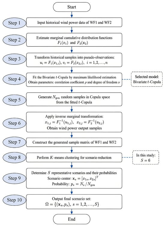
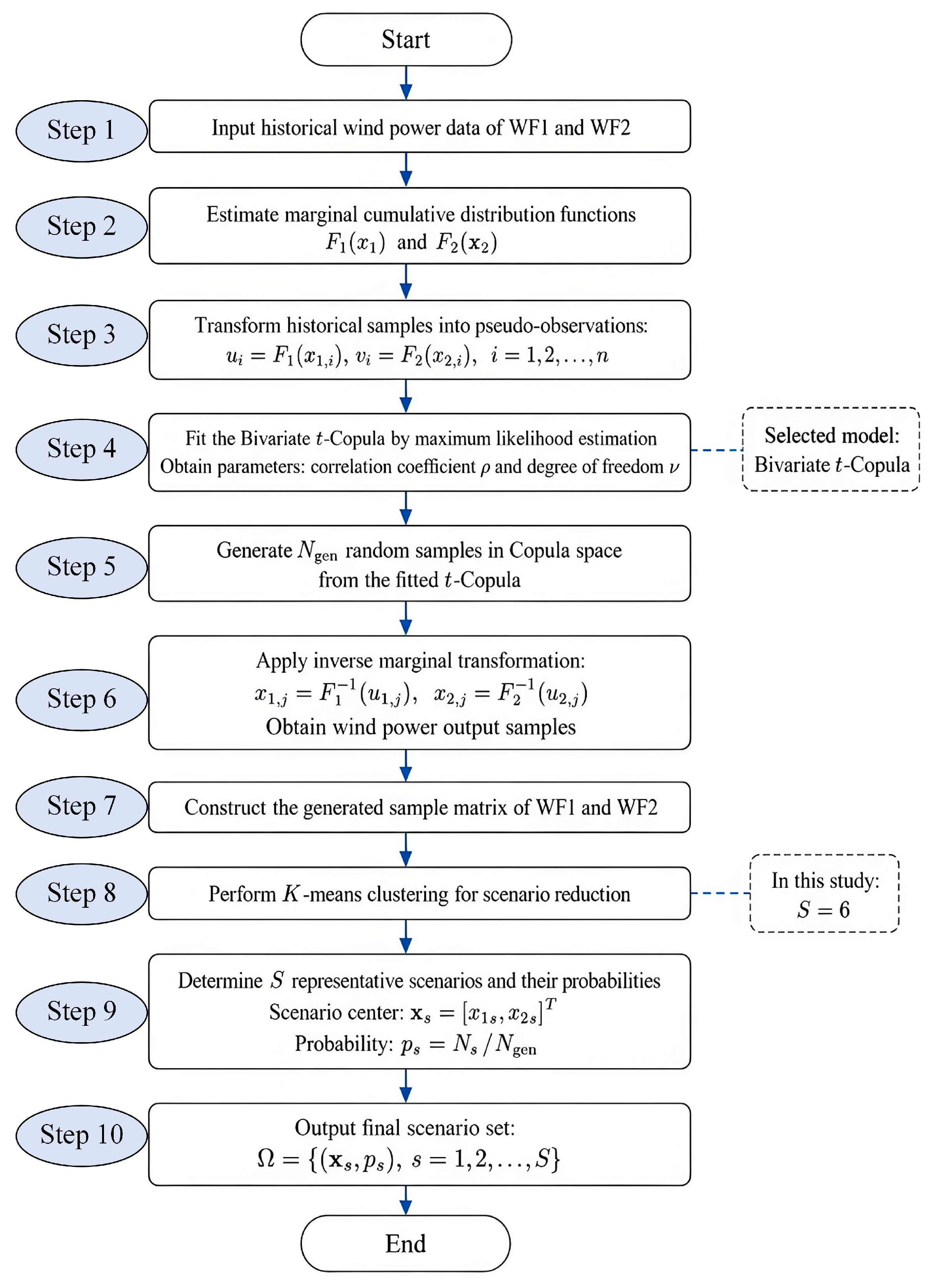
As illustrated in Figure 5, the proposed t-Copula-based wind power scenario generation procedure consists of marginal distribution estimation, t-Copula parameter identification, random sample generation in the Copula space, inverse marginal transformation, and K-means-based scenario reduction.

Figure 5. Flowchart of the t-Copula-based wind power scenario generation procedure.

4.3. Calculation Results

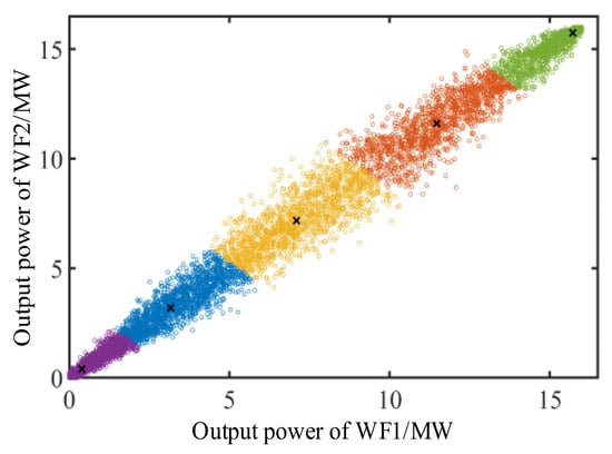
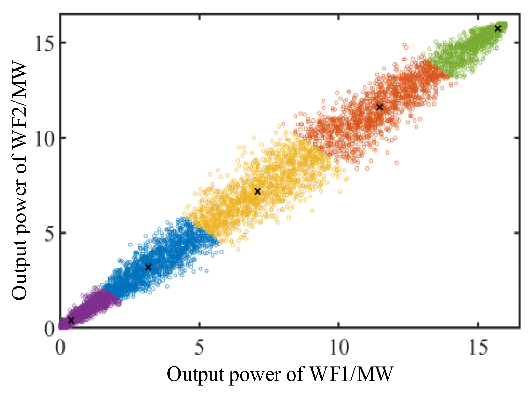
Based on the measured wind power data of WF1 and WF2, the Bivariate t-Copula model selected in the previous section is used to generate stochastic wind power scenarios. A total of 100,000 samples satisfying the fitted t-Copula distribution are first generated in the Copula space. Then, the K-means clustering method is adopted to reduce the generated samples into six representative scenarios. The cluster centers in the Copula space are denoted by u and v, and the corresponding wind power scenarios are obtained through the inverse transformation of the marginal distribution functions.

After the random samples are generated from the fitted Bivariate t-Copula and transformed into the original wind power output space, the K-means clustering method is adopted to reduce the generated samples into representative scenarios. The clustering result is shown in Figure 6, where the horizontal axis represents the output power of WF1 and the vertical axis represents the output power of WF2. Each point denotes one generated joint output state of the two wind farms, while the black crosses represent the cluster centers obtained by K-means clustering, which are used as the representative wind power scenarios. The generated samples are mainly distributed along a clear diagonal band, indicating a strong positive dependence between the outputs of WF1 and WF2. It can also be observed that the selected scenario centers cover the low-output, medium-output, and high-output regions, demonstrating that the reduced scenario set preserves the main joint variation characteristics of the generated wind power samples.

Figure 6. Scenario reduction results of t-Copula-generated joint wind power samples based on K-means clustering.

The generated representative scenarios and their probabilities are listed in Table 4.

Table 4. Generated wind power scenarios based on the Bivariate t-Copula.

Category	Variable	Scenario 1	Scenario 2	Scenario 3	Scenario 4	Scenario 5	Scenario 6
Copula function	u	0.0805	0.2452	0.4132	0.5733	0.7311	0.9048
	v	0.0804	0.2457	0.4134	0.5724	0.7310	0.9047
	Probability	0.1628	0.1678	0.1650	0.1576	0.1653	0.1815
Wind power/MW	WF1	0.0000	1.5516	4.0774	7.6384	12.0550	15.8010
	WF2	0.0018	1.5534	4.0887	7.6688	12.1860	15.8240
	Probability	0.1628	0.1678	0.1650	0.1576	0.1653	0.1815

As shown in Table 4, the representative scenarios cover the full output range from near-zero wind power to high wind power. Scenario 1 corresponds to the low-output condition, while Scenario 6 represents the high-output condition of the two wind farms. The intermediate scenarios describe different medium-output levels. Therefore, the reduced scenario set can retain the main distribution characteristics of the original generated samples.

The obtained Copula centers of u and v are very close in all scenarios. This result is consistent with the strong positive correlation identified in the parameter estimation and model evaluation results. It indicates that WF1 and WF2 tend to exhibit synchronized output variations under similar meteorological conditions. In other words, low-output and high-output states are likely to occur simultaneously in the two wind farms, rather than independently.

The probabilities of the six scenarios are also relatively balanced, ranging from 0.1576 to 0.1815. This means that the scenario reduction process does not lead to an excessive concentration of probability in a single scenario. The probability of Scenario 6 is slightly higher than the others, indicating that the high-output state has a relatively larger occurrence probability in the generated sample set. However, the difference among scenario probabilities is not significant, and the generated scenario set can provide a balanced representation of different wind power output levels.

From the perspective of wind power dispatching and stochastic optimization, the generated scenarios provide a compact description of the uncertain joint output of WF1 and WF2. The low-output scenarios can be used to evaluate the reserve requirement and power balance risk, while the high-output scenarios can be used to analyze wind power accommodation and possible curtailment conditions. Therefore, the obtained scenario set can support the subsequent optimization and operation analysis of power systems with two correlated wind farms.

4.4. Quantitative Evaluation of Generated Scenarios

To further evaluate the quality of the generated representative scenarios, several quantitative metrics are introduced to compare the reduced scenario set with the historical wind power samples. These metrics are used to assess whether the generated scenarios can preserve the marginal distribution characteristics, joint distribution similarity, statistical moments, and dependence structure of the original WF1 and WF2 output data.

Let the historical wind power samples be denoted by H = {(x_1i,x_2i)}_{i = 1}ⁿ, and let the reduced scenario set be denoted by Ω = {(x₁^s,x₂^s), p_s}_{s = 1}^S, where p_s is the probability of the s-th representative scenario. For each wind farm, the first-order Wasserstein distance is used to evaluate the marginal distribution deviation between the historical samples and the reduced scenarios:

$$W_{1,k}=W_1(\widehat{F}H,k,\widehat{F}\mathsf{\Omega },k),\hspace{1em}k=1,2$$

(36)

where ${\widehat{F}}_{H,k}$ and ${\widehat{F}}_{\mathsf{\Omega },k}$ denote the empirical marginal distribution of the historical samples and the weighted marginal distribution of the reduced scenarios, respectively. A smaller Wasserstein distance indicates better preservation of the marginal distribution.

The Kullback–Leibler divergence is adopted to measure the similarity between the joint probability distributions of the historical samples and the generated scenarios. The joint distributions are estimated using the same two-dimensional histogram bins, and a small positive constant ε is introduced to avoid zero-probability bins:

$$D_{\mathrm{KL}}(P|Q)={\displaystyle \sum _a{\displaystyle \sum _b(P_{ab}+\epsilon )}}\ln {\displaystyle \frac{P_{ab}+\epsilon }{Q_{ab}+\epsilon }}$$

(37)

where P_ab and Q_ab are the joint probabilities of the historical samples and the reduced scenarios in the (a,b)-th bin, respectively. A smaller value of D_KL(P||Q) indicates a higher similarity between the two joint distributions.

To evaluate statistical moment preservation, the relative errors of the mean and standard deviation are calculated as

$$e_{\mu ,k}={\displaystyle \frac{|{\mu }_{\mathsf{\Omega },k}-{\mu }_{\mathcal{H},k}|}{\left|{\mu }_{\mathcal{H},k}\right|}}\times 100\%,\hspace{1em}{e}_{\sigma ,k}={\displaystyle \frac{|{\sigma }_{\mathsf{\Omega },k}-{\sigma }_{\mathcal{H},k}|}{\left|{\sigma }_{\mathcal{H},k}\right|}}\times 100\%,\hspace{1em}k=1,2$$

(38)

where μ_H,k and σ_H,k are the mean and standard deviation of the historical samples, while μ_H,k and σ_H,k are the probability-weighted mean and standard deviation of the reduced scenarios.

In addition, the preservation of the dependence structure between WF1 and WF2 is evaluated by the absolute errors of Pearson, Spearman, and Kendall coefficients:

$$\Delta c=\left|c_{\mathsf{\Omega }}-c_H\right|$$

(39)

where c represents the Pearson correlation coefficient, Spearman coefficient, or Kendall coefficient. A smaller value of Δc indicates that the reduced scenarios better retain the dependence structure of the original wind power data.

The quantitative evaluation results are summarized in Table 5. It can be observed that the generated representative scenarios maintain small marginal distribution deviations, limited statistical moment errors, and small dependence-preservation errors. This demonstrates that the proposed t-Copula-based scenario generation and reduction procedure can effectively retain the main probabilistic and dependence characteristics of the historical two-wind-farm output data.

Table 5. Quantitative evaluation of the generated representative scenarios.

Evaluation Aspect	Metric	WF1	WF2	Joint/Dependence
Marginal distribution preservation	Wasserstein distance/MW	0.3185	0.3027	—
Joint distribution similarity	Kullback–Leibler divergence	—	—	0.9047
Moment preservation	Mean relative error/%	0.63	0.58	—
	Standard deviation relative error/%	2.41	2.36	—
Dependence preservation	Pearson coefficient error	—	—	0.0027
	Spearman coefficient error	—	—	0.0007
	Kendall coefficient error	—	—	0.0022

It can be observed from Table 5 that the generated representative scenarios maintain small marginal distribution deviations, limited statistical moment errors, and small dependence-preservation errors. This demonstrates that the proposed t-Copula-based scenario generation and reduction procedure can effectively retain the main probabilistic and dependence characteristics of the historical two-wind-farm output data.

4.5. Sensitivity Analysis of Sample Size and Scenario Number

To justify the selection of the number of generated samples and retained representative scenarios, a sensitivity analysis is conducted with respect to N_gen and S. The number of generated samples affects the statistical stability of the Copula-based random sampling process, while the number of retained scenarios determines the balance between scenario representation accuracy and OPF computational burden. In this study, the average Wasserstein distance, moment-preservation error, dependence-preservation error, and expected operating-cost deviation are used as evaluation indicators.

The average Wasserstein distance is calculated as:

$${\overline{W}}_1={\displaystyle \frac{1}{2}}\left(W_{1,1}+W_{1,2}\right)$$

(40)

where W_1,1 and W_1,2 are the Wasserstein distances of WF1 and WF2, respectively. The average moment-preservation error is defined as

$$e_{\mathrm{mom}}={\displaystyle \frac{1}{4}}{\displaystyle \sum _{k=1}^2}\left(e_{\mu ,k}+e_{\sigma ,k}\right)$$

(41)

where e_μ,k and e_σ,k denote the relative errors of the mean and standard deviation of the k-th wind farm. The dependence-preservation error is calculated by averaging the absolute errors of Pearson, Spearman, and Kendall coefficients:

$$e_{\mathrm{dep}}={\displaystyle \frac{1}{3}}\left(\Delta c_{\mathrm{Pearson}}+\Delta c_{\mathrm{Spearman}}+\Delta c_{\mathrm{Kendall}}\right)$$

(42)

In addition, the expected operating-cost deviation is used to evaluate the influence of scenario reduction on the OPF-WS application:

$$e_{\mathrm{cost}}={\displaystyle \frac{\left|F_{\mathsf{\Omega }}-F_{\mathrm{ref}}\right|}{F_{\mathrm{ref}}}}\times 100\%$$

(43)

where F_Ω is the probability-weighted expected operating cost obtained from the reduced scenario set, and F_ref is the reference expected operating cost obtained from a larger scenario set.

Based on the above indicators, the sensitivity of the generated sample size is first analyzed by varying N_gen from 10,000 to 200,000 while keeping the number of retained scenarios fixed at S = 6. The results are summarized in Table 6.

Table 6. Sensitivity analysis with respect to the number of generated samples.

Ngen	Average Wasserstein Distance [MW]	Moment-Preservation Error [%]	Dependence- Preservation Error	Expected Cost Deviation [%]
10,000	0.5264	2.76	0.0048	2.14
50,000	0.3792	1.88	0.0028	1.19
100,000	0.3106	1.50	0.0019	0.74
200,000	0.2974	1.42	0.0017	0.68

As shown in Table 6, increasing N_gen improves the statistical stability of the generated samples. When N_gen increases from 10,000 to 100,000, the average Wasserstein distance decreases from 0.5264 MW to 0.3106 MW, the moment-preservation error decreases from 2.76% to 1.50%, and the dependence-preservation error decreases from 0.0048 to 0.0019. However, when N_gen further increases from 100,000 to 200,000, the improvement becomes relatively limited. The expected cost deviation only decreases from 0.74% to 0.68%, indicating that the OPF-oriented results have become stable. Therefore, N_gen = 100,000 is selected to balance sampling stability and computational efficiency.

Furthermore, to evaluate the influence of the retained scenario number, N_gen is fixed at 100,000, and the number of representative scenarios, S, is varied from 4 to 10. The corresponding results are listed in Table 7.

Table 7. Sensitivity analysis with respect to the number of retained scenarios.

S	Average Wasserstein Distance [MW]	Moment-Preservation Error [%]	Dependence-Preservation Error	Number of OPF Subproblems
4	0.4628	2.37	0.0036	4
6	0.3106	1.50	0.0019	6
8	0.2743	1.28	0.0016	8
10	0.2529	1.16	0.0014	10

The influence of the retained scenario number S is shown in Table 7. Increasing S improves the representation accuracy of the reduced scenario set, as reflected by the decreasing Wasserstein distance, moment-preservation error, and dependence-preservation error. However, a larger S also increases the number of deterministic OPF subproblems. Compared with S = 4, retaining 6 scenarios significantly improves the scenario quality, while the improvement becomes more moderate when S increases from 6 to 8 or 10. Therefore, S = 6 is selected in this study as a reasonable compromise between scenario representation accuracy and OPF computational burden.

5. Application Case of the Generated Scenarios

5.1. OPF-WS Model

To further verify the effectiveness of the generated wind power scenarios in power system operation, the representative scenarios obtained by the t-Copula-based scenario generation method are introduced into an optimal power flow model with wind scenarios, denoted as the OPF-WS model. The purpose of the OPF-WS model is to determine the optimal dispatching scheme of conventional generators under different wind power output scenarios while satisfying the security constraints of the power system.

In the conventional OPF model, wind power outputs are usually treated as uncertain variables. In this study, the uncertainty of wind power is represented by the generated discrete scenarios. For each scenario, the wind power outputs of WF1 and WF2 are taken as known inputs, and the corresponding optimal dispatching result of conventional generators is obtained.

The objective function is to minimize the total fuel cost of conventional generating units. Since the generation cost of wind power is not considered in this study, the optimization objective is expressed as

$$F=\min {\displaystyle \sum _{i\in S_G}\left(a_{2i}{P}_{Gi}^2+a_{1i}{P}_{Gi}+a_{0i}\right)}$$

(44)

where P_Gi is the active power output of the i-th conventional generator; a_0i, a_1i, and a_2i are the fuel cost coefficients of the generator; and S_G denotes the set of conventional generators.

The OPF-WS model is subject to the following constraints:

$$\left\{\begin{array}{l}{P}_{Gi}+P_{Wi}^s-P_{Di}-U_i{\displaystyle \sum _{j=1}^n{U}_j\left(G_{ij}\cos {\theta }_{ij}+B_{ij}\sin {\theta }_{ij}\right)=0, i\in S_B}\hfill \\ Q_{Gi}+Q_{Wi}^s-Q_{Di}-U_i{\displaystyle \sum _{j=1}^n{U}_j\left(G_{ij}\cos {\theta }_{ij}-B_{ij}\sin {\theta }_{ij}\right)=0, i\in S_B}\hfill \\ {\underset{\_}{P}}_{Gi}\le P_{Gi}\le {\overline{P}}_{Gi}, i\in S_G\hfill \\ {\underset{\_}{P}}_{Wi}\le P_{Wi}^s\le {\overline{P}}_{Wi}, i\in S_W\hfill \\ {\underset{\_}{Q}}_{Ri}\le Q_{Ri}\le {\overline{Q}}_{Ri}, i\in S_R\hfill \\ {\underset{\_}{U}}_i\le U_i\le {\overline{U}}_i, i\in S_B\hfill \\ \left|P_L\right|\le {\overline{P}}_L, L\in S_L\hfill \end{array}\right.$$

(45)

where S_B is the set of system buses; S_G is the set of conventional generators; S_W is the set of wind farms; S_R is the set of reactive power compensation devices; and S_L is the set of transmission lines. P_Di and Q_Di denote the active and reactive loads at bus i, respectively. P_Wi^s and Q_Wi^s are the active and reactive wind power injections under the s-th scenario. U_i and θ_i are the voltage magnitude and phase angle of bus i, respectively, and θ_ij = θ_i − θ_j. G_ij and B_ij are the conductance and susceptance elements of the bus admittance matrix. The symbols with upper and lower bars denote the upper and lower limits of the corresponding variables.

In (45), the first two equations represent the active and reactive power balance constraints at each bus. The remaining inequalities represent the active power output limits of conventional generators, the wind power output limits, the reactive power limits, the bus voltage limits, and the transmission line power flow constraints. For each wind power scenario generated in the previous section, the corresponding wind power outputs P_Wi^s are substituted into the OPF-WS model, and the optimal generation dispatching scheme can be obtained.

It should be noted that the OPF-WS model used in this paper is a steady-state stochastic dispatch model rather than a time-domain dynamic model of wind turbine/converter systems. The generated wind power scenarios are used as scenario-dependent active power injections of WF1 and WF2. Reactive power injections and bus voltages are considered through the OPF power-balance equations, reactive power limits, voltage limits, and line-flow constraints. However, internal wind turbine and converter dynamic variables, such as rotor speed and DC-link voltage, are not included in the present model. Therefore, the following case study focuses on the applicability of the generated scenarios for steady-state dispatch analysis, rather than on the dynamic robust responses of wind farm control systems.

5.2. Calculation Results

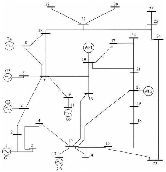
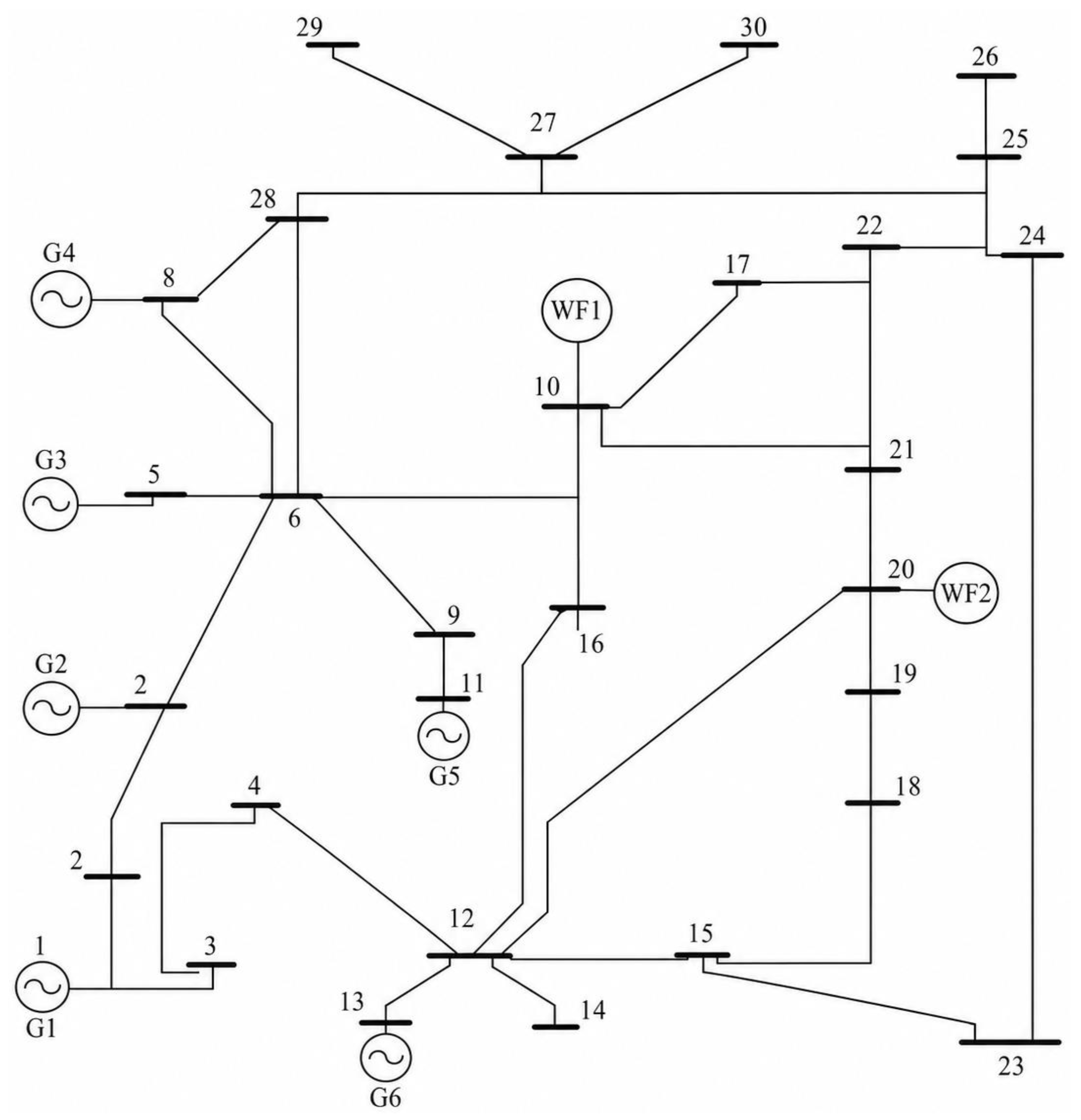
The IEEE 30-bus system is used as the test system to evaluate the applicability of the generated wind power scenarios in power system dispatch. The two wind farms, WF1 and WF2, are connected to bus 10 and bus 20, respectively, as shown in Figure 7. The historical wind power data of WF1 and WF2 are used to construct the t-Copula model, and the representative wind power scenarios obtained in Section 4.3 are introduced into the OPF-WS model.

Figure 7. Graph of the IEEE 30-bus system (WF1 and WF2 are connected to bus 10 and bus 20, respectively. The detailed branch parameters, including r_l, x_l, b_l, and S_lmax, are listed in Appendix A, Table A3, according to the corresponding from-bus and to-bus pairs.).

To improve the reproducibility of the case study, the main model-system parameters and simulation settings are summarized in Table 8. The generated wind power scenarios listed in Table 4 are used as active power injections of WF1 and WF2 in the OPF-WS model. Except for the added wind power injections, the standard IEEE 30-bus system settings are retained, including the bus data, branch data, generator limits, voltage limits, and generation cost coefficients. The detailed IEEE 30-bus system data are provided in the Supplementary Materials to facilitate replication by peers.

Table 8. Reproducibility settings of the case study.

Category	Parameter	Setting
Wind farm data	Wind farms	WF1 and WF2
	WF1 location	E 114°01′24″, N 41°30′01″
	WF2 location	E 114°27′36″, N 41°59′24″
	Installed capacity	WF1: 30.1 MW; WF2: 31.2 MW
	Wind power unit	MW
Marginal distribution	Estimation method	Non-parametric estimation
	Pseudo-observations	ui = FX(xi), vi = FY(yi)
Copula modeling	Candidate Copula models	Gaussian, t, Empirical, Frank, Clayton, and Gumbel Copulas
	Selected Copula model	Bivariate t-Copula
	Correlation coefficient	ρ = 0.9986
	Degree of freedom	v = 1.0000
Scenario generation	Number of generated samples	Ngen = 100,000
	Number of retained scenarios	S = 6
	Scenario probabilities	Calculated by the proportion of samples in each scenario
Scenario reduction	Reduction method	K-means clustering
	Number of clusters	6
	Scenario ordering	From low-output to high-output states
OPF-WS test system	Test system	Standard IEEE 30-bus system
	Base power	100 MVA
	Wind farm connection buses	WF1: bus 10; WF2: bus 20
	Conventional generators	Six conventional generators
	Generator active-power limits	PGimin ≤ PGi ≤ PGimax; detailed values are listed in Table A1
	Generator reactive-power limits	QGimin ≤ QGi ≤ QGimax; detailed values are listed in Table A1
	Voltage limits	Vimin ≤ Vi ≤ Vimax; detailed bus voltage limits are listed in Table A2
	Branch flow limits	Sl ≤ Slmax; detailed branch limits are listed in Table A3
	Generation cost coefficients	Quadratic coefficients a2i, a1i, and a0i are listed in Table A4
Implementation	Software environment	MATLAB2018a
	Random seed	2026

Figure 7 shows the topology of the IEEE 30-bus system with two wind farms. The generated wind power scenarios reflect different joint output levels of WF1 and WF2, including low-output, medium-output, and high-output operating conditions. Therefore, they can be used to evaluate the dispatching performance of the power system under different wind power fluctuation states.

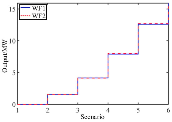
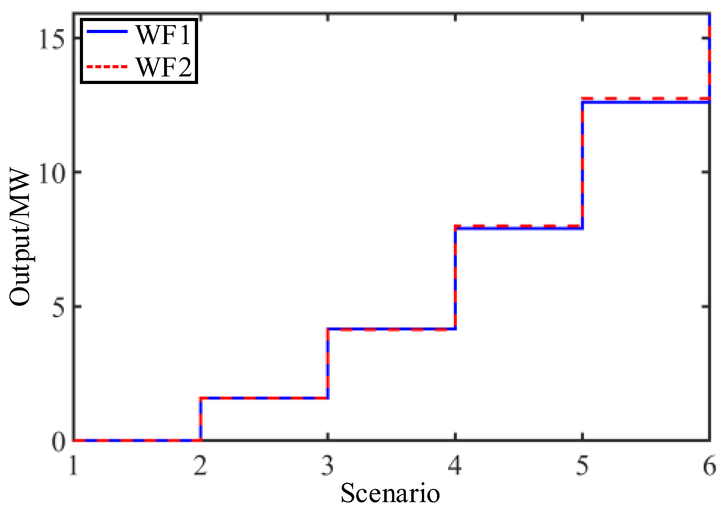
The generated scenarios shown in Figure 8 are substituted into the OPF-WS model one by one. For each scenario, the active power outputs of WF1 and WF2 are fixed according to the corresponding scenario values, and the conventional generator outputs are optimized by solving the OPF problem. The calculation results are summarized in Table 9.

Figure 8. Generated wind power scenarios of WF1 and WF2.

Table 9. Computing results.

Scenario	G1 [p.u.]	G2 [p.u.]	G3 [p.u.]	G4 [p.u.]	G5 [p.u.]	G6 [p.u.]	WF1 [MW]	WF2 [MW]
Scenario 1	0.2962	0.2491	0.7584	0.5017	0.7485	0.2986	0.0056	0.0088
Scenario 2	0.2906	0.2445	0.7445	0.4918	0.7336	0.2927	1.5894	1.5788
Scenario 3	0.2819	0.2373	0.7226	0.4768	0.7102	0.2842	4.1574	4.1385
Scenario 4	0.2690	0.2265	0.6901	0.4545	0.6755	0.2715	7.9069	8.0055
Scenario 5	0.2532	0.2132	0.6497	0.4269	0.6325	0.2558	12.6014	12.7397
Scenario 6	0.2424	0.2041	0.6225	0.4087	0.6036	0.2459	15.8986	15.9191
Max *	0.2424	0.2041	0.6225	0.4087	0.6036	0.2459	15.8986	15.9191
Min *	0.2962	0.2491	0.7584	0.5017	0.7485	0.2986	0.0056	0.0088
E *	0.2721	0.2291	0.6977	0.4598	0.6837	0.2745	7.0376	7.0761

* Max denotes the scenario with the maximum total wind power output of WF1 and WF2 among all generated scenarios; Min denotes the scenario with the minimum total wind power output of WF1 and WF2 among all generated scenarios; E denotes the expected value of each variable over all generated scenarios.

From the calculation results in Table 8, it can be observed that the generated wind power scenarios have a direct influence on the optimal dispatching results of conventional generators. When the wind power output is low, as in Scenario 1, WF1 and WF2 only provide 0.0056 MW and 0.0088 MW, respectively. Under this condition, the conventional generators are required to supply more active power to satisfy the system load demand. For example, the outputs of G3, G5, and G6 reach 0.7584 p.u., 0.7485 p.u., and 0.2986 p.u., respectively.

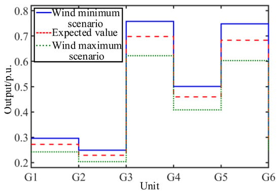
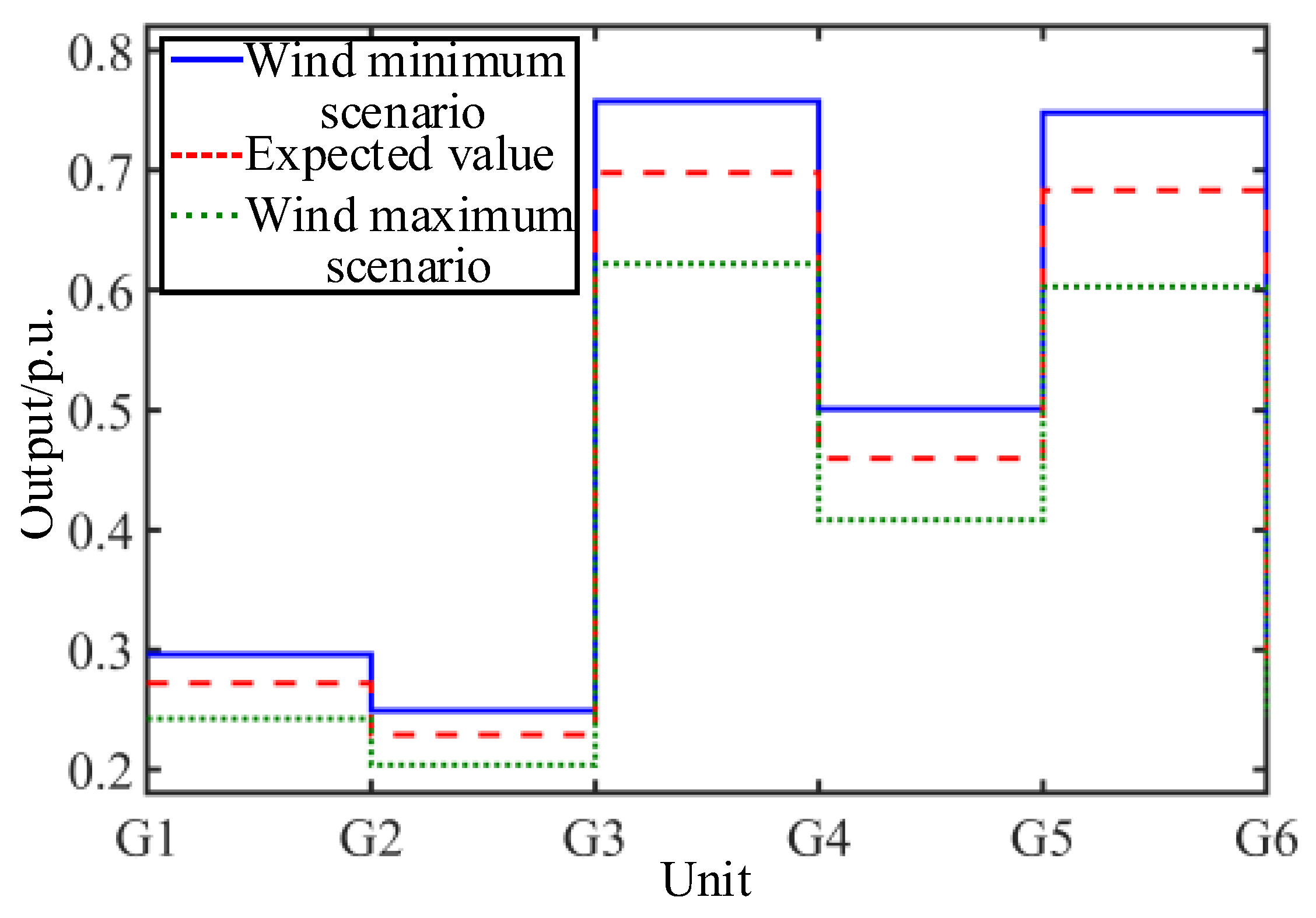
The Max and Min rows in Table 8 correspond to the maximum and minimum wind power output scenarios, respectively. It should be noted that the maximum wind power scenario leads to relatively lower conventional generator outputs, whereas the minimum wind power scenario requires higher conventional generator outputs. The expected output row E gives the probability-weighted average dispatching result under all generated scenarios. For instance, the expected outputs of G1, G3, and G5 are 0.2721 p.u., 0.6977 p.u., and 0.6837 p.u., respectively, while the expected wind power outputs of WF1 and WF2 are 7.0376 MW and 7.0761 MW.

Figure 9 further illustrates the dispatching variation in conventional generators under different wind power conditions. The generator outputs under the minimum wind power scenario are generally higher than those under the maximum wind power scenario, and the expected dispatching curve lies between these two boundary conditions. This result shows that the generated scenarios can effectively reflect the influence of wind power uncertainty on conventional unit dispatch.

Figure 9. Unit output of each scene.

To further evaluate the practical value of the generated scenarios, several operational performance indicators are introduced in addition to the generator dispatch results. For the s-th wind power scenario, the total operating cost is calculated using the OPF objective function:

$$F_s=\sum _{i\in S_G}\left(a_{2i}{P}_{Gi,s}^2+a_{1i}{P}_{Gi,s}+a_{0i}\right)$$

(46)

where P_Gi,s is the active power output of the i-th conventional generator under the s-th scenario. The total active network loss is calculated as:

$$P_{\mathrm{loss},s}=\sum _{i\in S_G}{P}_{Gi,s}+\sum _{i\in S_W}{P}_{Wi,s}-\sum _{i\in S_B}{P}_{Di}$$

(47)

where P_Wi,s is the wind power injection under the s-th scenario, and P_Di is the active load at bus i. The wind power penetration ratio is defined as:

$${\eta }_{W,s}={\displaystyle \frac{{\displaystyle \sum _{i\in S_W}}{P}_{Wi,s}}{{\displaystyle \sum _{i\in S_B}}{P}_{Di}}}\times 100\%$$

(48)

To describe the voltage profile and transmission loading condition, the voltage deviation index and maximum branch loading ratio are further defined as:

$${\mathrm{VD}}_s={\displaystyle \frac{1}{N_B}}\sum _{i\in S_B}\left|U_{i,s}-1\right|$$

(49)

$${\lambda }_s^{\max }=\underset{l\in S_L}{\max }{\displaystyle \frac{\left|S_{l,s}\right|}{S_l^{\max }}}\times 100\%$$

(50)

where N_B is the number of buses, U_i,s is the voltage magnitude of bus i, S_l,s is the apparent power flow of branch l, and S_l^max is the corresponding branch flow limit. The calculated operational performance indicators are summarized in Table 10.

Table 10. Operational performance indicators under different wind power scenarios.

Scenario	Total Wind Power [MW]	Operating Cost [$/h]	Active Network Loss [MW]	Wind Penetration [%]	Voltage Deviation Index	Maximum Branch Loading [%]
Scenario 1	0.0144	1212.83	2.18	0.01	0.0224	76.31
Scenario 2	3.1682	1179.27	2.05	1.12	0.0215	74.82
Scenario 3	8.2959	1127.87	1.88	2.93	0.0202	72.36
Scenario 4	15.9124	1053.33	1.64	5.61	0.0187	69.41
Scenario 5	25.3411	963.90	1.42	8.94	0.0178	66.53
Scenario 6	31.8177	905.94	1.36	11.23	0.0172	64.87
Expected value	14.1137	1070.71	1.75	4.98	0.0196	70.63

As shown in Table 10, the operating cost decreases as the total wind power output increases, which is consistent with the reduction in conventional generator output. However, the additional indicators provide more detailed operational information. The active network loss varies with the spatial distribution and magnitude of wind power injections, indicating that different wind power scenarios may lead to different power flow patterns. The wind power penetration ratio increases from low-output scenarios to high-output scenarios, while the voltage deviation index and maximum branch loading ratio remain within acceptable ranges. This demonstrates that the generated representative scenarios can be used not only to reflect the uncertainty of wind power output, but also to evaluate its influence on economic dispatch, network losses, voltage profiles, and transmission loading conditions.

From the perspective of stochastic operation, the expected-value row provides a probability-weighted assessment of system performance under the generated scenario set. Therefore, the proposed t-Copula-based scenario generation method can provide useful scenario inputs for OPF-WS analysis and support more comprehensive operational decision-making under wind power uncertainty.

Therefore, the t-Copula-based scenario generation method can provide representative wind power inputs for the OPF-WS model. By substituting the generated scenarios into the optimal power flow calculation, the uncertainty of WF1 and WF2 is transformed into a finite number of deterministic dispatching cases. This provides a practical basis for evaluating unit output adjustment, reserve requirements, and secure operation of power systems with two correlated wind farms.

6. Conclusions

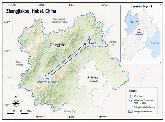
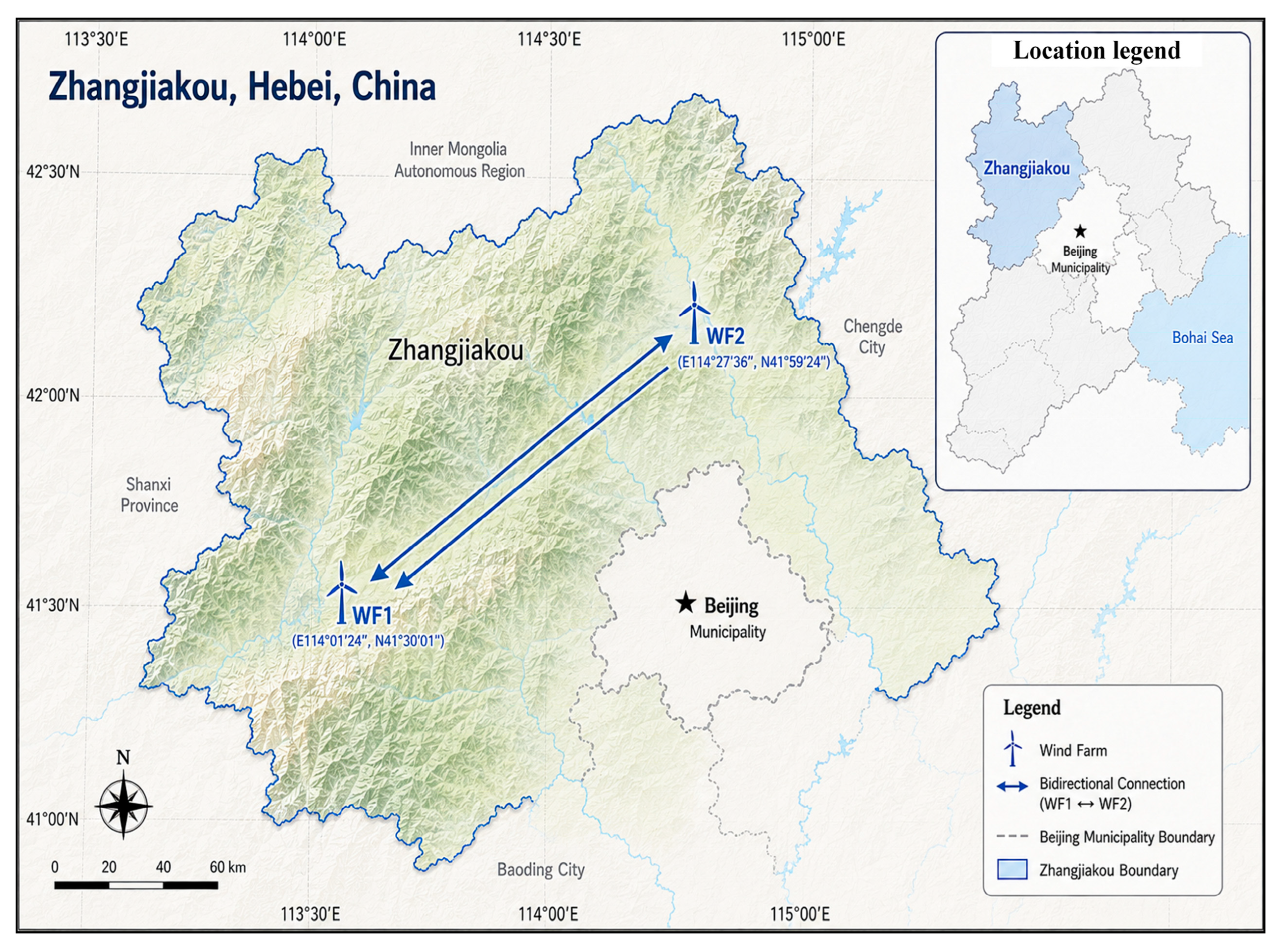
This paper proposes a Copula-based scenario generation method for two correlated wind farms’ output and applies it to stochastic operation analysis of power systems. Based on the measured output data of WF1 and WF2 in Zhangjiakou, northern Hebei, the marginal cumulative distribution functions are obtained through non-parametric estimation. Then, six Copula tools are compared to characterize the dependence structure between the two wind farms, including Gaussian Copula, t-Copula, Empirical Copula, Frank Copula, Clayton Copula, and Gumbel Copula.

The fitting results show that WF1 and WF2 have a strong positive dependence. Among the parametric Copula models, the Bivariate t-Copula achieves the smallest fitting distance from the Empirical Copula and shows good consistency in correlation, Spearman, and Kendall indicators. Therefore, the Bivariate t-Copula is selected as the preferred model for scenario generation. Based on the fitted t-Copula, random samples are generated in the Copula space and transformed into wind power output samples through inverse marginal distribution functions, from which a finite set of representative scenarios and corresponding probabilities are obtained.

The generated scenarios are further introduced into the OPF-WS model based on the IEEE 30-bus system. The calculation results show that different wind power scenarios directly affect the dispatching results of conventional generators. As wind power output increases, the required active power output of conventional units decreases accordingly. Therefore, the proposed t-Copula-based scenario generation method can provide representative wind power inputs for stochastic dispatch and support unit output adjustment, reserve assessment, and secure operation of power systems with two correlated wind farms.

Although the present study focuses on two adjacent wind farms and adopts a Bivariate t-Copula model, the proposed scenario-generation workflow provides a basis for higher-dimensional and spatio-temporal extensions. Future work will investigate multivariate t-Copulas, Vine Copulas, VARMA-Copula models, and deep generative approaches to model larger wind farm clusters with more complex spatial and temporal dependence structures. In addition, the generated scenarios can be further combined with detailed wind turbine and converter dynamic models to evaluate the robust responses of active power, reactive power, rotor speed, DC-link voltage, and terminal voltage under wind power and grid disturbances.

References

- Dahal, S.; Hegglid, G.J.; Kristiansen, J.; Chhetri, B.B.; Mishra, S.; Oyvang, T. Integrating multiple slack bus operations and metaheuristic techniques for power flow optimization. Sci. Rep. 2025, 15, 16821. [Google Scholar] [CrossRef] [Scilit] [PubMed]
- Jin, W.; Wang, P.; Yuan, J. Key role and optimization dispatch research of technical virtual power plants in the new energy era. Energies 2024, 17, 5796. [Google Scholar] [CrossRef] [Scilit]
- Zhan, Y.; Wang, L.; Xie, X. Wind power integration capacity analysis considering sub/super-synchronous oscillation stability constraint. IEEE Trans. Ind. Appl. 2025, 61, 2782–2790. [Google Scholar] [CrossRef] [Scilit]
- Carlucci, S.; Erba, S.; Pagliano, L.; de Dear, R. ASHRAE likelihood of dissatisfaction: A new right-here and right-now thermal comfort index for assessing the likelihood of dissatisfaction according to the ASHRAE adaptive comfort model. Energy Build. 2021, 250, 111286. [Google Scholar] [CrossRef] [Scilit]
- Liu, X. Economic load dispatch constrained by wind power availability: A wait-and-see approach. IEEE Trans. Smart Grid 2010, 1, 347–355. [Google Scholar] [CrossRef] [Scilit]
- Hooda, P.; Prakash, P. Enhanced risk-based strategy for microgrid market participation using three-stage stochastic optimization. J. Electr. Eng. Technol. 2025, 21, 315–336. [Google Scholar] [CrossRef] [Scilit]
- López-Garza, E.; Domínguez-Cruz, R.F.; Martell-Chávez, F.; Salgado-Tránsito, I. Fuzzy logic and linear programming-based power grid-enhanced economical dispatch for sustainable and stable grid operation in Eastern Mexico. Energies 2022, 15, 4069. [Google Scholar] [CrossRef] [Scilit]
- Shufian, A.; Shib, S.K.; Dipto, D.R.; Rahman, M.T.; Hannan, N.; Fattah, S.A. Fuzzy logic-controlled three-phase dynamic voltage restorer for enhancing voltage stabilization and power quality. Int. J. Electr. Power Energy Syst. 2025, 166, 110517. [Google Scholar] [CrossRef] [Scilit]
- Chen, Y.; Wang, D.; Li, J.; Fan, H.; Li, J.; Luo, D.; Li, L. A SSSC optimal configuration method to enhance available transfer capability considering multi-wind farm access. IET Renew. Power Gener. 2023, 17, 3777–3792. [Google Scholar] [CrossRef] [Scilit]
- Baas, P.; Verzijlbergh, R.; van Dorp, P.; Jonker, H. Investigating energy production and wake losses of multi-gigawatt offshore wind farms with atmospheric large-eddy simulation. Wind Energy Sci. 2023, 8, 787–805. [Google Scholar] [CrossRef] [Scilit]
- Al-Duais, F.S.; Al-Sharpi, R.S. A unique Markov chain Monte Carlo method for forecasting wind power utilizing time series model. Alex. Eng. J. 2023, 74, 51–63. [Google Scholar] [CrossRef] [Scilit]
- Abdoos, A.A.; Abdoos, H.; Kazemitabar, J.; Mobashsher, M.M.; Khaloo, H. An intelligent hybrid method based on Monte Carlo simulation for short-term probabilistic wind power prediction. Energy 2023, 278, 127914. [Google Scholar] [CrossRef] [Scilit]
- Shao, B.; Zhao, S.; Gao, B.; Yang, Y.; Blaabjerg, F. Adequacy of the single-generator equivalent model for stability analysis in wind farms with VSC-HVDC systems. IEEE Trans. Energy Convers. 2021, 36, 907–918. [Google Scholar] [CrossRef] [Scilit]
- Zhang, W.; Wang, Y.; Zeeshan, M.; Han, F.; Song, K. Super-twisting sliding mode control of grid-side inverters for wind power generation systems with parameter perturbation. Int. J. Electr. Power Energy Syst. 2025, 165, 110501. [Google Scholar] [CrossRef] [Scilit]
- Silveira, F.V.J.; Gomes-Silva, F.; de Brito, C.R.; Jale, J.S.; de Gusmao, F.R.S.; Xavier, S.F.A., Jr.; Rocha, J.S. Modelling wind speed with a univariate probability distribution depending on two baseline functions. Hacet. J. Math. Stat. 2023, 52, 808–827. [Google Scholar] [CrossRef] [Scilit]
- Sharma, K.C.; Gupta, A.; Bhakar, R. Wind power scenario generation considering spatiotemporal correlations: A distribution free hybrid VARMA-Copula approach. Smart Grids Sustain. Energy 2023, 8, 17. [Google Scholar] [CrossRef] [Scilit]
- Zhang, J.; Guo, Y.; Dong, Y.; Bastidas-Arteaga, E. Coupling aerodynamic wake effects with corrosion-fatigue degradation for system-level reliability assessment of floating offshore wind farms. Renew. Energy 2026, 269, 125884. [Google Scholar]
- Zhu, X.; Xiao, H.; Zhu, L.; Li, Y.; Gao, X.; Sun, Q.; Wang, H. A graph neural model for predicting wind speed behavior based on the effect of wind speed point coupling. Energy 2025, 336, 138174. [Google Scholar] [CrossRef] [Scilit]
- Wang, X.; Zhou, J.S.; Qin, B.; Guo, L.Z. Coordinated power smoothing control strategy of multi-wind turbines and energy storage systems in wind farm based on MADRL. IEEE Trans. Sustain. Energy 2024, 15, 368–380. [Google Scholar] [CrossRef] [Scilit]
- Zhang, D.; Xie, X.; Hao, Z.; Liu, W.; Han, X.; Li, Q. A regular-vine copula-based evidence theory model for structural reliability analysis involving multidimensional parameter correlation. Comput. Meth. Appl. Mech. Eng. 2025, 444, 118152. [Google Scholar] [CrossRef] [Scilit]
- Song, C.; Yuan, Y.; Dai, L. Distributionally robust optimization of virtual power plant bidding strategies considering discrete scenario-based uncertainties in day-ahead market prices and wind powers. Electr. Power Syst. Res. 2025, 248, 111977. [Google Scholar] [CrossRef] [Scilit]
- Ye, L.; Peng, Y.S.; Li, Y.L.; Li, Z. A novel informer-time-series generative adversarial networks for day-ahead scenario generation of wind power. Appl. Energy 2024, 364, 123182. [Google Scholar] [CrossRef] [Scilit]
- Zhang, Z.; Sun, Z.; Guo, H.; Guo, P.; Yang, X.; Yang, P. Short-term multi-step wind power prediction model based on Pt-Transformer neural network integrating spatio-temporal feature and sparse attention. Electr. Power Syst. Res. 2025, 248, 111970. [Google Scholar] [CrossRef] [Scilit]
- Zhang, H.; Zandehshahvar, R.; Tanneau, M.; Van Hentenryck, P. Weather-informed probabilistic forecasting and scenario generation in power systems. Appl. Energy 2025, 384, 125369. [Google Scholar] [CrossRef] [Scilit]
- Tan, J.; Zhang, J.; Liu, H.; Lan, B. A high dimensional uncertain scenario generating method for wind power and photovoltaic considering spatiotemporal correlation. Energy 2025, 340, 139224. [Google Scholar] [CrossRef] [Scilit]
- Zhao, W.; Shao, Z.; Yang, S.; Lu, X. A novel conditional diffusion model for joint source-load scenario generation considering both diversity and controllability. Appl. Energy 2025, 377, 124555. [Google Scholar] [CrossRef] [Scilit]
- Dong, X.; Sun, Y.; Yang, Y.; Mao, Z. Controllable renewable energy scenario generation based on pattern-guided diffusion models. Appl. Energy 2025, 398, 126446. [Google Scholar] [CrossRef] [Scilit]
- Kuschinski, N.; Jara, A. Grid-uniform copulas and rectangle exchanges: Bayesian model and inference for a rich class of copula functions. Bayesian Anal. 2025, 20, 1357–1384. [Google Scholar] [CrossRef] [Scilit]
- Bai, Z.; Wei, H.; Xiao, Y.; Song, S.; Kucherenko, S. A vine copula-based global sensitivity analysis method for structures with multidimensional dependent variables. Mathematics 2021, 9, 2489. [Google Scholar] [CrossRef] [Scilit]
- Ansari, J.; Rüschendorf, L. Sklar’s theorem, copula products, and ordering results in factor models. Depend. Model. 2021, 9, 267–306. [Google Scholar] [CrossRef] [Scilit]
- Li, Q.; Ni, P.H.; Du, X.L.; Han, Q. Bayesian model updating with variational inference and Gaussian copula model. Comput. Methods Appl. Mech. Eng. 2025, 438, 117842. [Google Scholar] [CrossRef] [Scilit]
- Wang, Z.Y.; Dong, Z.L. How does the time-varying network structure evolve between the EU carbon futures prices and industrial and energy-related indices? A study based on a time-varying t-copula. Int. J. Energy Res. 2023, 2023, 6696059. [Google Scholar] [CrossRef] [Scilit]
- Sreekumar, S.; Sharma, K.C.; Bhakar, R. Gumbel copula based aggregated net load forecasting for modern power systems. IET Gener. Transm. Distrib. 2018, 12, 4348–4358. [Google Scholar] [CrossRef] [Scilit]
- Adu-Ntim, J.K.; Omari-Sasu, A.Y.; Boateng, M.A.; Mensah, I.A. A novel bivariate regression model derived from the Clayton copula and the Odd Dagum-G family and its application. Sci. Afr. 2025, 28, e02761. [Google Scholar] [CrossRef] [Scilit]
- Lin, S.F.; Liu, C.T.; Shen, Y.W.; Li, F.X.; Li, D.D.; Fu, Y. Stochastic planning of integrated energy system via Frank-Copula function and scenario reduction. IEEE Trans. Smart Grid 2022, 13, 202–212. [Google Scholar] [CrossRef] [Scilit]
- Inan, G.E. Parameter estimation for doubly geometric process with inverse Gaussian distribution and its applications. Fluct. Noise Lett. 2025, 24, 4. [Google Scholar] [CrossRef] [Scilit]
- Bücher, A.; Pakzad, C. The empirical copula process in high dimensions: Stute’s representation and applications. Ann. Stat. 2025, 53, 2462–2487. [Google Scholar] [CrossRef] [Scilit]
Disclaimer/Publisher’s Note: The statements, opinions and data contained in all publications are solely those of the individual author(s) and contributor(s) and not of MDPI and/or the editor(s). MDPI and/or the editor(s) disclaim responsibility for any injury to people or property resulting from any ideas, methods, instructions or products referred to in the content. |
© 2026 by the authors. Licensee MDPI, Basel, Switzerland. This article is an open access article distributed under the terms and conditions of the Creative Commons Attribution (CC BY) license.