From Energy Flow Regimes to Regime Dynamics: A Window-Based Hidden Markov Modeling Framework for Photovoltaic–Building Systems

Abstract

High-resolution measurement data from photovoltaic–building systems enable analyses that extend beyond static energy balances toward the temporal structure of system operation. This study proposes a window-based analytical pipeline to identify operating regimes and their dynamic transitions in an integrated PV–building energy system. The approach combines energy flow decomposition, sliding temporal windows, and hidden Markov modeling to capture short-term behavioral patterns, regime persistence, and transition pathways. The results indicate that system operation is dominated by a limited number of persistent regimes with a pronounced diurnal organization. Regime transitions are structured and directional, typically occurring through intermediate operating states rather than via abrupt switching between energetically extreme conditions. The analysis of regime residence times reveals distinct characteristic temporal scales associated with different operating modes. Overall, the proposed framework provides a process-oriented representation of PV–building system dynamics that enhances interpretability and supports advanced monitoring and analysis of integrated energy systems.

1. Introduction

The integration of photovoltaic generation into building energy systems has intensified the need for analytical methods capable of capturing not only aggregate energy performance, but also the dynamic allocation of energy between local consumption, surplus export, and grid import [1,2]. Traditional performance indicators, such as self-consumption ratios or monthly energy balances, provide limited insight into the temporal organization of system operation [3]. In practice, PV–building systems evolve through a sequence of characteristic operating modes driven by the interaction between time-varying photovoltaic generation and building demand [4].

Recent studies have introduced the concept of energy flow regimes [5,6] as a system-oriented representation of photovoltaic–building operation, identifying characteristic configurations of autoconsumption, surplus, and grid import using unsupervised clustering techniques [7]. While such approaches successfully reveal recurring operating states, they typically rely on point-wise representations of system behavior, treating individual time steps as independent observations [8]. As a result, temporal structure is reconstructed a posteriori and remains weakly coupled to the regime identification process itself [9].

However, system operation is inherently process-based. Regimes persist for finite durations, transitions occur in preferred directions, and daily operation follows repeatable temporal trajectories rather than random switching between states [10]. Capturing these properties requires analytical frameworks that explicitly incorporate temporal context into the definition of operating regimes.

Hidden Markov models (HMMs) are widely used for identifying latent regimes in sequential and stochastic processes across multiple scientific domains [11]. In financial economics, HMMs are applied to detect market regimes and model volatility dynamics in equity and macroeconomic indicators [12]. In risk and actuarial sciences, regime-switching HMM frameworks enable the modeling of extreme events and time-varying risk structures [13]. In logistics and supply chain systems, HMMs are used to represent dynamic operational states and transitions in complex production and distribution processes [14]. In intelligent transportation and smart city applications, HMM-based approaches support route prediction, mobility pattern analysis, and adaptive decision-making [15]. In signal processing and speech recognition, HMMs remain a standard tool for modeling temporal sequences with hidden state structures [16]. In biological and ecological systems, HMMs are used to describe behavioral states and transitions in observed time series [17]. Recent methodological developments extend classical HMMs toward hybrid and neural formulations, allowing more flexible representation of nonlinear and multiscale dynamics [18]. These diverse applications demonstrate that HMM provides a general and robust framework for regime detection and temporal structure analysis, which motivates its use in the present study of photovoltaic–building energy interactions. In the energy domain, HMM-based approaches have also been applied to photovoltaic systems for fault detection and performance monitoring [19,20]. These diverse applications demonstrate that HMM provides a general and robust framework for regime detection and temporal structure analysis, which motivates its use in the present study of photovoltaic–building energy interactions.

In this study, we propose a window-based regime modeling pipeline that extends energy flow regime analysis from static state identification toward probabilistic process modeling. By representing system behavior over short temporal windows and employing hidden Markov models, the proposed framework enables the identification of latent behavioral regimes characterized by persistence, transition asymmetry, and time-of-day structure. The approach is computationally efficient, interpretable, and compatible with high-resolution building energy data, making it suitable for both research and operational applications.

A growing body of literature demonstrates that advanced sequence modeling techniques such as hidden Markov models are increasingly transferred across disciplinary boundaries and successfully applied to complex real-world systems. This cross-domain adoption reflects the general capability of such models to reveal latent regimes, temporal persistence, and structured transitions in stochastic processes. The present study follows this line of research by adapting regime-based modeling to photovoltaic–building energy interactions.

The contribution of this work is not the introduction of a new hidden Markov model, but the development of a physically interpretable analytical framework that integrates energy-flow decomposition, window-based feature extraction, and probabilistic regime modeling for the short-term analysis of PV–building operation.

2. Data and Energy Flow Representation

2.1. Monitored PV–Building System and Measurement Data

The monitored system is a grid-connected photovoltaic–building installation located at the WSEI University campus in Lublin, Poland. The analyzed building is an administrative and educational facility with a variable electricity demand profile resulting from daily academic, office, lighting, ventilation, and auxiliary electrical loads. This type of load profile is characterized by strong intra-day variability, with demand peaks occurring mainly during working hours and substantially lower demand during nighttime periods. The combination of a predictable photovoltaic generation profile and a non-uniform building load creates frequent temporal mismatches between local production and electricity demand, making the system suitable for regime-based analysis of energy flow dynamics.

The photovoltaic system is installed on the flat roof of the building at the fourth-floor level. The installation has a nominal peak capacity of approximately 50 kWp and has been in continuous operation since February 2023. It consists of 108 monocrystalline single-sided photovoltaic modules, each rated at 460 Wp, resulting in a total installed DC capacity of 49,680 Wp. The modules are mounted with a tilt angle of 15° and arranged in two symmetric orientations. One group of 54 modules is oriented at an azimuth of 116°, while the remaining 54 modules are oriented at an azimuth of 206°. This east–southeast and south–southwest configuration supports a broader daily production profile by distributing generation between morning and afternoon periods. The rooftop location and surrounding installation geometry limit significant shading effects under normal operating conditions.

The PV array is connected to a three-phase grid-connected inverter with a nominal AC power of 50 kW. The system is equipped with module-level power optimizers, installed for every second photovoltaic module. This configuration enables panel-level performance monitoring, comparison of module operation, and partial mitigation of mismatch losses. The use of optimizers also supports fault diagnostics and improves the reliability of the monitored production data. The inverter is integrated with an IoT-based monitoring platform, which records photovoltaic generation and communicates with the associated metering infrastructure.

Building electricity demand is measured using a smart metering system installed at the main electrical connection point of the building. The measurement system provides a synchronized time series of photovoltaic generation and total building electricity demand. Both signals are aggregated to fixed 15-min intervals and aligned to common timestamp boundaries. This synchronization is essential because the subsequent energy flow decomposition requires photovoltaic production and building demand to refer to the same time step. The 15-min resolution was selected because it is sufficiently detailed to capture intra-day changes in both photovoltaic production and building load, while remaining consistent with typical building energy monitoring practice.

The analyzed dataset covered the full month of March 2025. This period includes complete daily cycles of photovoltaic generation and building demand and therefore enables the identification of recurring operating regimes, regime persistence, and transition patterns. The photovoltaic production profile exhibits a clear diurnal structure, with near-zero generation during nighttime hours and distinct daytime production peaks. In contrast, the building load profile is more irregular and reflects the operational behavior of an administrative and educational building. The mismatch between production and demand leads to alternating periods of local self-consumption, surplus export to the grid, and electricity import from the grid.

Before further analysis, the raw measurement data were subjected to a deterministic preprocessing procedure. First, the production and consumption time series were checked for timestamp consistency and aligned on the common 15-min sampling grid. Second, physically implausible values were identified and removed. Negative photovoltaic generation values and values exceeding the technically plausible range of the installation were treated as erroneous. Third, the internal consistency of the measured and derived variables was verified using the instantaneous power balance between photovoltaic generation, building demand, self-consumption, surplus export, and grid import.

Missing or inconsistent observations were negligible in the analyzed dataset. Only isolated data points required correction, and these were replaced using linear interpolation between adjacent valid observations. The share of corrected records was below 1% of the monthly dataset and therefore did not affect the temporal structure of the analyzed energy flows. After preprocessing, the dataset formed a continuous and physically consistent time series suitable for window-based feature extraction and hidden Markov modeling.

The monitored variables used directly in the analysis were photovoltaic power generation and total building electricity demand. Based on these two primary signals, three derived energy flow components were calculated at each time step: on-site photovoltaic self-consumption, surplus photovoltaic generation exported to the grid, and electricity imported from the grid. These three components provide an internally consistent description of instantaneous energy allocation within the PV–building system. In the proposed modeling framework, they form the physical basis for identifying operating regimes and interpreting their temporal transitions.

2.2. Measurement Data

The analysis was based on high-resolution measurement data collected from a photovoltaic-equipped administrative building during March 2025. The dataset includes time series of photovoltaic power generation and total building electricity consumption sampled at a 15-min resolution. This temporal granularity is sufficient to capture intra-day variability in both generation and demand while remaining consistent with standard building energy monitoring practices [21].

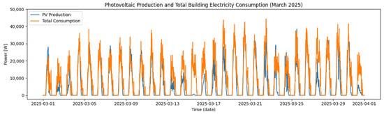
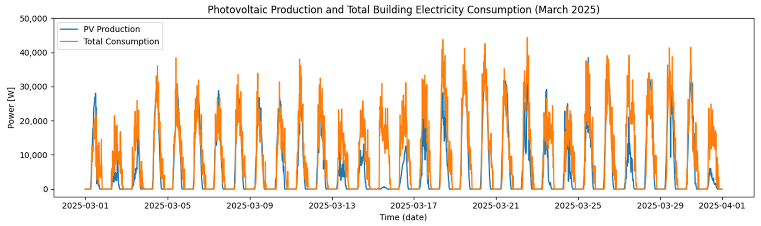
Figure 1 presents the time series of photovoltaic power production and total building electricity consumption recorded at a 15-min resolution during March 2025. The photovoltaic generation exhibits a pronounced diurnal pattern with clearly defined daily peaks and near-zero values during nighttime hours. In contrast, the electricity consumption profile is characterized by irregular high-power events and substantial intra-day variability, which do not directly follow the production pattern.

Figure 1. Time series of photovoltaic power production and total building electricity consumption recorded at a 15-min resolution in March 2025 [22].

The simultaneous visualization of production and consumption highlights periods of significant mismatch between locally generated energy and building demand, resulting in alternating phases of grid electricity import and surplus photovoltaic export [23]. This temporal heterogeneity, combined with the strong daily structure of photovoltaic generation, indicates that system operation cannot be adequately described using point-wise observations alone. Instead, short-term temporal context is required to capture characteristic operational behavior, providing motivation for the window-based regime analysis introduced in the following section.

2.3. Energy Flow Decomposition

From the measured production and consumption signals, three internally consistent energy flow components were derived at each time step: autoconsumption, surplus photovoltaic generation, and grid electricity import. Autoconsumption represents the portion of photovoltaic energy directly used by the building, surplus denotes photovoltaic generation exceeding instantaneous demand and exported to the grid, and grid import corresponds to electricity drawn from the grid when local generation is insufficient. Together, these variables form a complete description of instantaneous energy allocation within the PV–building system.

By focusing on energy flows rather than raw production and consumption, the analysis emphasizes system behavior as the outcome of allocation processes. Each time step can thus be interpreted as a point in a multidimensional energy flow space describing how energy is routed between local use and the grid.

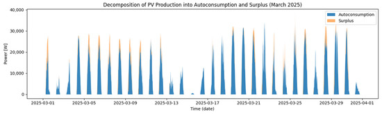
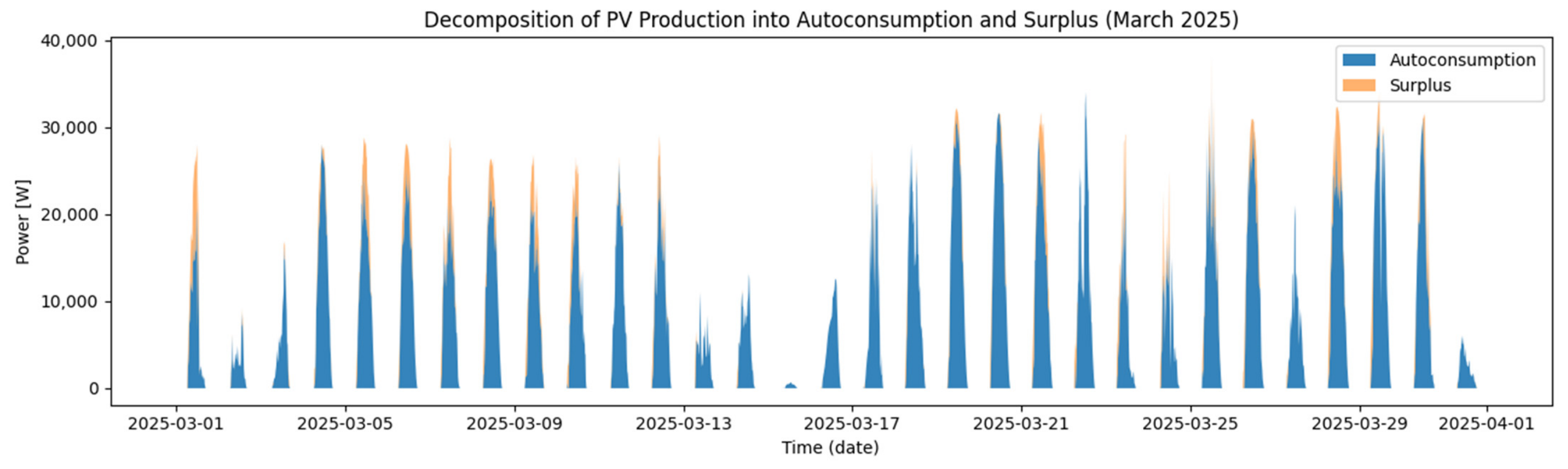
Figure 2 illustrates the decomposition of photovoltaic power production into autoconsumption and surplus export. The stacked representation highlights how locally generated energy is either directly utilized by the building or exported to the grid, depending on the instantaneous balance between production and demand [24]. Periods of high photovoltaic generation lead to an increase in surplus export once local demand is saturated, while during lower production levels, the majority of generated energy is consumed on-site. This decomposition provides a physically consistent basis for defining energy flow regimes analyzed in subsequent sections.

Figure 2. Decomposition of photovoltaic power production into autoconsumption and surplus export at a 15-min resolution for March 2025.

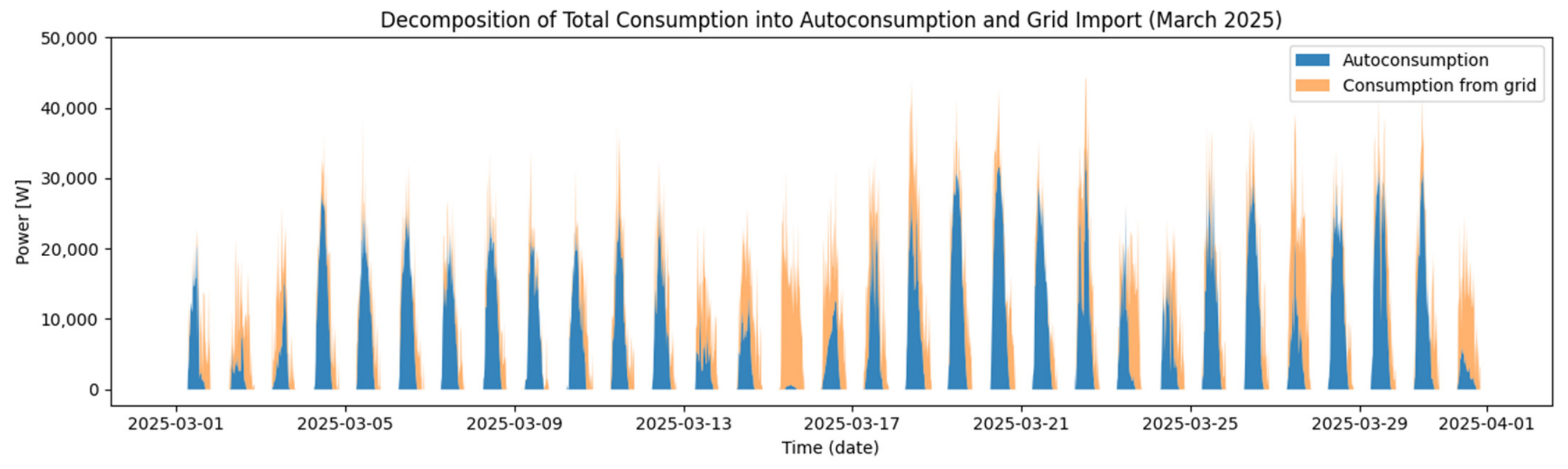
Figure 3 presents the decomposition of total building electricity consumption into autoconsumption and grid import. The stacked representation highlights that the building demand is partially supplied by locally generated photovoltaic energy when available, while the remaining portion is covered by electricity imported from the grid. Periods of negligible photovoltaic production (e.g., nighttime) correspond to grid-dominant consumption, whereas during daylight hours, the autoconsumption component increases and reduces grid dependency. Together with the production-side decomposition (Figure 2), this demand-side decomposition provides a complete, internally consistent energy flow representation used in the subsequent regime-based analysis.

Figure 3. Decomposition of total building electricity consumption into autoconsumption and grid electricity import at a 15-min resolution for March 2025.

The production-side and demand-side decompositions presented in Figure 2 and Figure 3 jointly provide a complete and physically consistent description of instantaneous energy allocation within the PV–building system. While these decompositions clearly identify the underlying energy flow components, they remain point-wise representations that do not capture the temporal organization of system operation. To address this limitation, the following section introduces a window-based analytical framework that explicitly incorporates short-term temporal context and enables the identification of persistent operational regimes and their dynamic transitions [25].

2.4. Scope and Rationale for the March Dataset

The analysis focused on March 2025 as a short-term methodological case study. In the climatic conditions of Poland, March represents a transitional period between winter and spring and is characterized by substantial intra-month variability in solar availability, ambient temperature, and daily weather patterns. The length of day and night is relatively balanced, while the month may include both winter-like and early-spring operating conditions. This makes March a particularly informative period for analyzing short-term changes in photovoltaic–building energy flow regimes.

The objective of this study is not to provide a complete seasonal assessment of the monitored PV–building system, but to investigate whether short-term regime dynamics can be identified and interpreted using a window-based hidden Markov modeling framework. From this perspective, March provides a compact but variable observation window in which different combinations of photovoltaic production and building electricity demand occur. These combinations lead to alternating periods of grid import, local self-consumption, surplus export, and intermediate operating states.

The March dataset should be interpreted as a deliberately selected transitional-period case study rather than as a representative annual dataset. The identified regime frequencies, residence times, and transition probabilities are specific to the analyzed building, PV system, and observation period. However, the proposed analytical framework is transferable to other high-resolution PV–building datasets, where the regime structure can be re-estimated for different seasons, building types, and photovoltaic capacities.

The March dataset was selected not as a substitute for seasonal validation, but as a compact transitional-period dataset suitable for testing whether the proposed method can describe the short-term variability of PV–building operating regimes.

The present study does not aim to provide an annual energy yield assessment, seasonal benchmarking, or long-term forecasting of photovoltaic production. Instead, its objective is to analyze short-term regime dynamics in PV–building energy flows. This distinction is important because operational energy management and control-oriented analysis are typically driven by variability occurring over minutes, hours, and daily cycles rather than by annual averages. In this context, March in Polish climatic conditions constitutes an informative transitional period. Day and night durations are relatively balanced, winter-like and spring-like days may occur within the same month, and relatively low ambient temperatures can still support efficient photovoltaic conversion during sunny periods. As a result, the analyzed month contains diverse short-term combinations of photovoltaic generation, building demand, grid import, self-consumption, and surplus export. Therefore, the March dataset was selected as a compact and variable observation window suitable for demonstrating the proposed window-based HMM framework for regime identification and transition analysis.

3. Window-Based Regime Modeling Pipeline

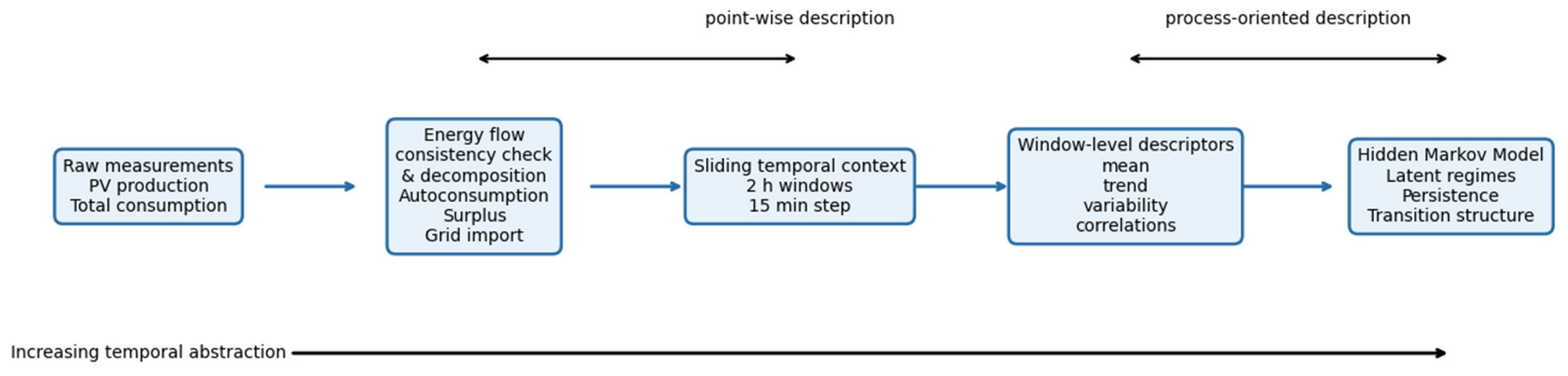
Figure 4 summarizes the proposed analytical pipeline used to model the dynamic operation of the photovoltaic–building system. Starting from high-resolution measurement data, energy flows are first decomposed into physically meaningful components, which are then analyzed over sliding temporal windows to capture short-term operational behavior. Window-level features are subsequently modeled using a hidden Markov model, enabling the identification of persistent operating regimes and their transition structure. The diagram emphasizes increasing temporal abstraction, from raw measurements and instantaneous energy allocation toward persistent operating regimes and their transition structure.

Figure 4. Overview of the proposed window-based analysis pipeline for identifying persistent energy flow regimes and their dynamic transitions in a photovoltaic–building system.

3.1. Temporal Windowing

Instead of analyzing individual time steps, system operation is represented using overlapping temporal windows of fixed duration. In this study, two-hour windows composed of eight consecutive 15-min samples were employed, with a sliding step of one sample [26]. Each window captures short-term temporal structure, including trends, variability, and interdependencies between energy flow components [27].

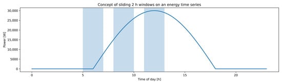
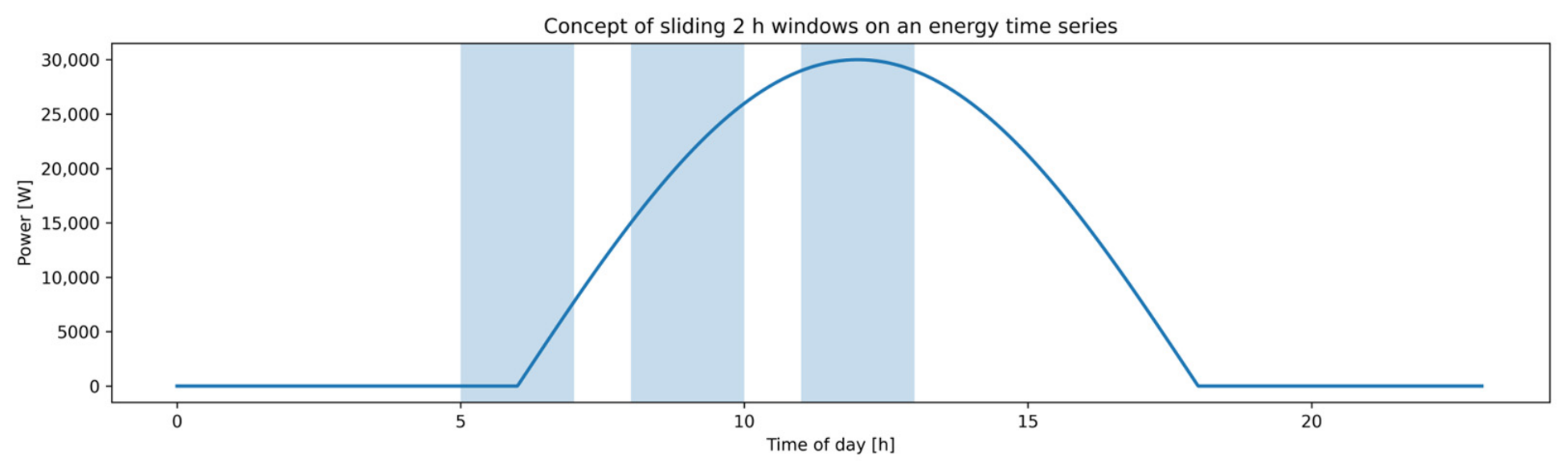
To incorporate short-term temporal context into the analysis, system operation is represented using overlapping time windows rather than individual time steps, as schematically illustrated in Figure 5.

Figure 5. Conceptual illustration of sliding 2 h windows applied to an energy time series. Each window captures short-term system behavior over a finite temporal context, enabling regime identification based on local dynamics rather than instantaneous power values.

3.2. Feature Extraction

For each temporal window, a set of descriptive features is computed, including mean values, standard deviations, linear trends, peak-to-peak amplitudes, and pairwise correlations between energy flow variables. These features provide a compact summary of window-level behavior and enable comparison between different segments of system operation.

For clarity, the main feature groups were calculated explicitly for each energy-flow variable. Let y_n,ℓ,m denote the value of the m-th energy-flow component in the n-th window at local sample ℓ, where m = 1, 2, 3 corresponds to self-consumption, surplus export, and grid import, and ℓ = 1, …, L. The mean value, standard deviation, peak-to-peak amplitude, and linear trend coefficient were calculated as:

$${\mu }_{n,m}={\displaystyle \frac{1}{L}}{\displaystyle \sum _{l=1}^L}{y}_{n,l,m}$$

$${\sigma }_{n,m}=\sqrt{{\displaystyle \frac{1}{L-1}}{\displaystyle \sum _{l=1}^L}{\left(y_{n,l,m}-{\mu }_{n,m}\right)}^2}$$

$$a_{n,m}={max}_l\left(y_{n,m,l}\right)-{min}_l\left(y_{n,m,l}\right)$$

$$b_{n,m}={\displaystyle \frac{{\sum }_{l=1}^L\left(l-\overline{l}\right)\left(y_{n,l,m}-{\mu }_{n,m}\right)}{{\sum }_{l=1}^L{\left(l-\overline{l}\right)}^2}}$$

where b_n,m denotes the slope of the least-squares linear trend within the window. Pairwise correlations between energy-flow components were calculated as:

$${\rho }_{n,mq}={\displaystyle \frac{{\sum }_{l=1}^L\left(y_{n,l,m}-{\mu }_{n,m}\right)\left(y_{n,l,q}-{\mu }_{n,q}\right)}{\sqrt{{\sum }_{l=1}^L{\left(y_{n,l,m}-{\mu }_{n,m}\right)}^2}\sqrt{{\sum }_{l=1}^L{\left(y_{n,l,q}-{\mu }_{n,q}\right)}^2}}}$$

for m,q ∈ {1, 2, 3} and m < q. The complete feature vector for each window was therefore defined as:

$$f_n=\left[{\mu }_{n,1:3},{\sigma }_{n,1:3},a_{n,1:3},b_{n,1:3},{\rho }_{n,12},{{\rho }_{n,13},\rho }_{n,23}\right]$$

This formulation produces a compact window-level representation containing information on the level, variability, local dynamics, and mutual relationships between the energy-flow components.

3.3. Dimensionality Reduction

The resulting feature vectors were standardized and projected onto a lower-dimensional space using principal component analysis (PCA) [28]. Dimensionality reduction serves to suppress noise, mitigate redundancy among features, and facilitate probabilistic modeling while preserving the dominant modes of variability in system behavior [29].

To formalize the transformation from the original time series to the HMM observation sequence, let

$$y_t={\left[P_{self}\left(t\right),P_{surplus}\left(t\right), P_{grid}\left(t\right)\right]}^T$$

denote the energy-flow vector at time step t, where t = 1, …, T. A sliding temporal window of length L samples and step s is defined as:

$$W_n=\left\{y_{\left(n-1\right)s+1},y_{\left(n-1\right)s+2},y_{\left(n-1\right)s+L}\right\}$$

where n = 1, …, N, L = 8 for the 2 h window, and s = 1 for the 15 min sliding step.

Each window W_n is transformed into a feature vector f_n containing statistical and dynamic descriptors of the energy-flow variables:

$$f_n=\left[\mu \left(W_n\right),\sigma \left(W_n\right),r\left(W_n\right),a\left(W_n\right),C\left(W_n\right)\right]$$

where μ(W_n), σ(W_n), r(W_n), a(W_n), and C(W_n) denote mean values, standard deviations, linear trends, peak-to-peak amplitudes, and pairwise correlations calculated within the window, respectively.

The feature matrix F = [f₁, …, f_N]^T is standardized and projected using PCA:

$$\tilde{F}={\displaystyle \frac{F-\overline{F}}{s_F}}$$

$$X=\tilde{F}{V}_d$$

where V_d contains the first d principal component loading vectors. The rows of X, denoted as x_n, form the observation sequence used by the HMM.

The number of retained principal components d was selected based on the cumulative explained variance ratio:

$${\eta }_d={\displaystyle \frac{{\sum }_{q=1}^d{\lambda }_q}{{\sum }_{q=1}^p{\lambda }_q}}$$

where λ_q denotes the eigenvalue associated with the q-th principal component and p is the original number of window-level features. The retained PCA representation was selected to preserve the dominant variability of the feature matrix while reducing redundancy before HMM estimation. In this study, the first d = 3 principal components were retained, explaining 64.89% of the total variance.

3.4. Hidden Markov Modeling

A hidden Markov model was employed to represent the sequence of window-level observations as emissions from a finite set of latent operating regimes. Each hidden state corresponds to a persistent behavioral regime, while the state transition matrix encodes the probabilities of moving between regimes. Model parameters were estimated using the expectation–maximization algorithm, and the most probable sequence of regimes was inferred using the Viterbi algorithm.

Formally, let x_n ∈ R^d denote the PCA-reduced feature vector extracted from the n-th temporal window, where n = 1, …, N. Each vector x_n represents the short-term behavior of the PV–building system within a sliding window. The corresponding hidden operating regime is denoted by z_n ∈ {1, …, K}, where K is the number of hidden states. In this study, K = 5 was selected based on the sensitivity analysis described in Section 3.5 and Section 4.1.

$$P\left(z_1=k\right)={\pi }_k$$

$$P(z_n=j│z_{n-1}=i)=A_{ij}$$

where π_k is the initial probability of regime k, and A_ij is the transition probability from regime i to regime j. The transition matrix A therefore provides a probabilistic description of regime persistence and regime-to-regime transitions.

The observation vector x_n is assumed to be generated conditionally on the hidden state z_n. In the Gaussian HMM formulation used in this study, the emission distribution for state k is defined as:

$$x_n|z_n=k~N\left({\mu }_k,{\Sigma }_k\right)$$

where μ_k and Σ_k denote the mean vector and covariance matrix of the emission distribution associated with hidden regime k. The full set of HMM parameters is therefore given by:

$$\theta ={\left\{\pi ,A,{\mu }_k,{\Sigma }_k\right\}}_{k=1}^K$$

The model parameters θ are estimated by maximizing the likelihood of the observed sequence of window-level feature vectors:

$$P\left(X|\theta \right)=\sum _{z_1,\cdots ,z_N}P\left(z_1\right){\displaystyle \prod _{n=2}^N}P\left(z_n|z_{n-1}\right){\displaystyle \prod _{n=1}^N}P\left(x_n|z_n\right)$$

where X = {x₁, …, x_N} denotes the complete sequence of window-level observations. Parameter estimation is performed using the expectation–maximization algorithm. After training, the most probable hidden regime sequence is inferred using the Viterbi algorithm:

$$\widehat{Z} = arg {max}_Z P(Z | X, \theta )$$

where

$$\widehat{Z}=\left\{{\widehat{z}}_1,\cdots ,{\widehat{z}}_{1N}\right\}$$

is the estimated sequence of PV–building operating regimes. Based on this sequence, regime occurrence frequency, residence times, self-transition probabilities, and transition pathways are calculated. Thus, the HMM formulation provides not only a classification of window-level operating conditions, but also a probabilistic description of their temporal persistence and evolution.

The occurrence frequency of regime k was calculated as:

$$F_k={\displaystyle \frac{1}{N}}{\displaystyle \sum _{n=1}^N}I\left({\widehat{z}}_n=k\right)$$

where I(⋅) is the indicator function. The empirical transition probability from regime i to regime j was calculated as:

$${\widehat{A}}_{ij}={\displaystyle \frac{{\sum }_{n=2}^{N}I\left({\widehat{z}}_{n-1}=i,{\widehat{z}}_n=j\right)}{{\sum }_{n=2}^{N}I\left({\widehat{z}}_{n-1}=i\right)}}$$

Residence times were calculated from consecutive runs of identical hidden states in the decoded sequence. If m_k,r denotes the number of consecutive windows assigned to regime k during the r-th residence episode, then the corresponding residence time is:

$${\tau }_{k,r}=m_{k,r}s∆t$$

where s is the sliding step and Δt = 15 min is the original sampling interval. The mean residence time for regime k was then obtained as:

$${\overline{\tau }}_k={\displaystyle \frac{1}{R_k}}{\displaystyle \sum _{r=1}^{R_k}}{\tau }_{k,r}$$

where R_k is the number of residence episodes assigned to regime k.

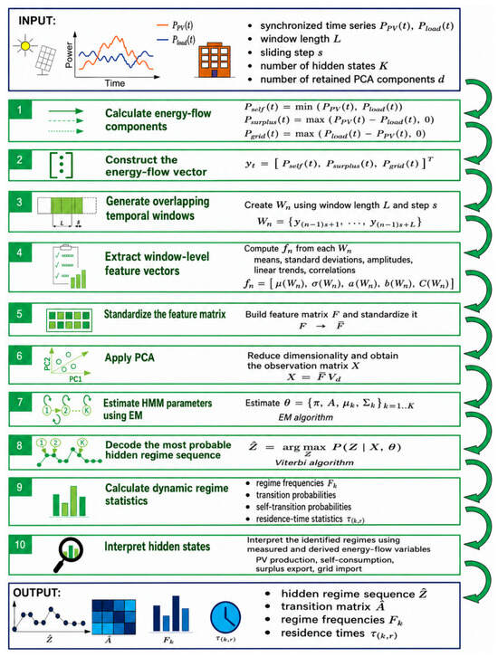
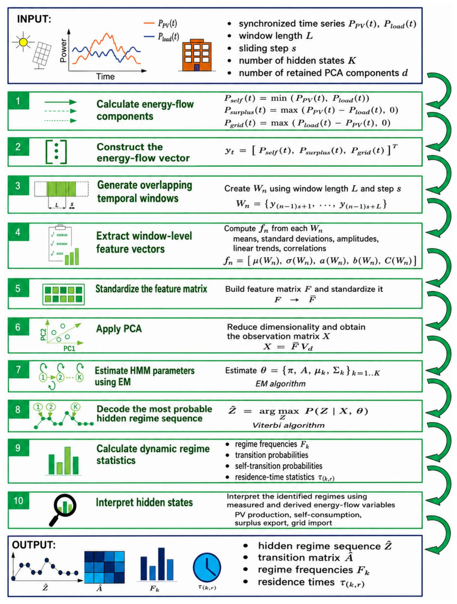
The complete computational workflow of the proposed approach is summarized in Figure 6. The diagram shows how the analysis proceeds from synchronized PV production and building load measurements to a probabilistic description of hidden operating regimes. It also clarifies the role of each processing stage, including energy-flow decomposition, temporal windowing, feature extraction, standardization, PCA transformation, HMM parameter estimation, Viterbi decoding, and the calculation of regime-level dynamic indicators. This workflow provides a transparent link between the measured electrical quantities and the final interpretation of PV–building regime persistence and transition dynamics.

Figure 6. Algorithmic workflow of the proposed window-based HMM pipeline for PV–building regime modeling. The pipeline transforms synchronized photovoltaic production and building load time series into physically interpretable energy-flow variables, constructs overlapping temporal windows, extracts and standardizes window-level features, applies PCA dimensionality reduction, estimates HMM parameters using the EM algorithm, decodes the most probable hidden regime sequence using the Viterbi algorithm, and calculates regime frequencies, transition probabilities, self-transition probabilities, and residence-time statistics. The final output is a probabilistic, process-oriented representation of PV–building operating regimes and their dynamic transitions.

Based on the workflow presented in Figure 6, together with the mathematical definitions and parameter settings provided in the preceding subsections, the computational methodology applied in this study can be reproduced in detail. The figure links all major processing stages, from the measured PV production and building load time series, through energy-flow decomposition, sliding-window construction, feature extraction, standardization and PCA transformation, to HMM estimation, Viterbi decoding, and the calculation of regime-level dynamic indicators. Therefore, the proposed pipeline is not only conceptually interpretable, but also computationally transparent and reproducible.

3.5. Parameter Selection and Sensitivity Analysis

The selection of the temporal window length, sliding step, and number of hidden states is an important methodological issue in window-based regime modeling. These parameters influence the temporal resolution of the analysis, the stability of the identified regimes, the structure of the transition matrix, and the resulting residence-time distributions. Therefore, a sensitivity analysis was performed to assess the robustness of the proposed configuration.

The original data were recorded at a 15 min resolution. Several window lengths were evaluated: 1 h, 1.5 h, 2 h, 3 h, and 4 h, corresponding to 4, 6, 8, 12, and 16 consecutive samples, respectively. The 15 min sliding step was used as the baseline because it preserves the native temporal resolution of the measurement system and allows gradual changes in the PV–building operation to be tracked without additional temporal aggregation. Additional step sizes of 30 min and 60 min were also tested to assess the effect of reduced overlap between consecutive windows.

For each parameter configuration, the HMM was estimated using different numbers of hidden states, ranging from 3 to 8. The resulting models were evaluated using several complementary criteria: model log-likelihood, information criteria, state separability in the PCA-reduced feature space, stability of the transition matrix, residence-time distributions, and physical interpretability of the identified regimes. Since the objective of the study is not only statistical segmentation, but also physically meaningful regime interpretation, the final parameter choice was based on a balance between quantitative model quality and the ability to distinguish interpretable PV–building operating modes.

Shorter windows, especially the 1 h variant, preserved high temporal resolution but produced more fragmented state sequences and less stable residence-time distributions. Such windows were sensitive to short-term fluctuations in building load and photovoltaic output, leading to rapid switching between states. In contrast, longer windows of 3 h and 4 h provided smoother regime sequences but partially suppressed morning and evening transition periods, which are important for interpreting the dynamic evolution of the system.

The 2 h window provided the most balanced representation. It contained eight consecutive 15 min samples, which was sufficient to compute meaningful window-level descriptors such as mean values, standard deviations, linear trends, amplitudes, and correlations. At the same time, it preserved the timing of intra-day transitions between grid-dominated, intermediate, autoconsumption-dominated, and photovoltaic-driven regimes. Therefore, the 2 h window was selected as a compromise between noise suppression, temporal resolution, and physical interpretability.

The sensitivity analysis of the number of hidden states showed that models with three or four states captured only the dominant operating modes but tended to merge physically distinct transition regimes. This reduced the ability of the model to describe gradual transitions between grid-dominated and photovoltaic-driven operation. Conversely, models with six or more states introduced additional low-frequency states that were difficult to interpret physically and did not substantially improve the description of regime persistence or transition pathways. The five-state model provided a stable and interpretable decomposition of PV–building operation, distinguishing zero or near-zero generation periods, grid-dominated load conditions, moderate photovoltaic contribution, export-related operation, and high photovoltaic production with simultaneous self-consumption and surplus export.

Consequently, the final configuration used in this study consisted of a 2 h sliding window, a 15 min sliding step, and five hidden states. This configuration was selected not as an arbitrary setting, but as a balanced solution that preserves short-term temporal dynamics while providing stable, physically interpretable regimes and meaningful transition and residence-time statistics.

4. Results

4.1. Parameter Sensitivity Analysis and Final Model Configuration

Before interpreting the identified operating regimes, a parameter sensitivity analysis was performed to justify the final configuration of the window-based HMM pipeline. The analysis focused on three methodological parameters that directly affect regime identification and temporal interpretation: the length of the sliding window, the sliding step, and the number of hidden states. These parameters influence the temporal resolution of the analysis, the stability of the resulting state sequence, the transition matrix, and the residence-time distributions.

First, the effect of window length was evaluated while keeping the sliding step fixed at 15 min and the number of hidden states fixed at five. Window lengths of 1 h, 1.5 h, 2 h, 3 h, and 4 h were tested. Each configuration was assessed using log-likelihood, AIC, BIC, Silhouette coefficient, mean self-transition probability, and mean residence time. The results are presented in Table 1.

Table 1. Sensitivity of the HMM results to the temporal window length.

Window Length	Step	States	N Windows	Log-Likelihood	AIC	BIC	Silhouette	Mean Self-Transition	Mean Residence Time
1.0 h	15 min	5	2973	4544.1	−8980.2	−8656.3	0.447	0.906	3.33 h
1.5 h	15 min	5	2971	3566.9	−7025.8	−6702.0	0.451	0.920	4.70 h
2.0 h	15 min	5	2969	2220.8	−4333.6	−4009.8	0.462	0.923	4.58 h
3.0 h	15 min	5	2965	−31.9	171.8	495.6	0.427	0.933	4.44 h
4.0 h	15 min	5	2961	−2520.0	5148.0	5471.5	0.394	0.936	4.60 h

The results indicate that the 2 h window provides the most balanced representation of short-term PV–building dynamics. Shorter windows preserve high temporal resolution but are more sensitive to short-term fluctuations in photovoltaic generation and building demand, leading to more fragmented state sequences. Longer windows increase temporal smoothing and self-transition probability, but they reduce the separability of regimes and weaken the visibility of morning and evening transition periods. The 2 h window achieved the highest silhouette value among the tested window lengths while maintaining high regime persistence and physically meaningful residence times.

Second, the sensitivity to the number of hidden states was assessed for the selected 2 h window and 15 min sliding step. The number of states was varied from three to eight. The results are summarized in Table 2.

Table 2. Sensitivity of the HMM results to the number of hidden states.

HMM States	N Windows	Log-Likelihood	AIC	BIC	Silhouette	Mean Self-Transition	Mean Residence Time	Low-Frequency States < 5%
3	2969	963.9	−1875.8	−1719.8	0.417	0.956	5.67 h	0
4	2969	1569.4	−3034.9	−2826.9	0.428	0.952	5.62 h	0
5	2969	2220.8	−4333.6	−4009.8	0.462	0.923	4.58 h	0
6	2969	3196.3	−6202.7	−5824.9	0.475	0.915	3.89 h	0
7	2969	3489.5	−6739.1	−6259.4	0.457	0.898	3.26 h	0
8	2969	3724.7	−7153.4	−6561.9	0.459	0.883	2.87 h	1

As expected, models with a larger number of hidden states achieved higher likelihood values because of their greater flexibility. However, increasing the number of states also led to shorter residence times and lower self-transition stability, indicating increasing fragmentation of the regime sequence. Models with three or four states captured only the dominant operating modes and tended to merge physically distinct intermediate states. In contrast, models with six or more states introduced additional subdivisions of already interpretable regimes, with limited added physical meaning. The eight-state model also produced a low-frequency state, suggesting the onset of over-segmentation.

The five-state model was therefore selected as a compromise between statistical quality, regime separability, residence-time stability, and physical interpretability. It preserves the main operating modes of the PV–building system while still allowing intermediate transition regimes to be identified.

Finally, the effect of the sliding step was assessed for the 2 h window and five hidden states. The 15 min step was retained because it preserves the native temporal resolution of the measurement data and provides the most continuous representation of regime evolution (see Table 3). Larger steps reduced the number of windows and weakened the continuity of the inferred state sequence, especially for transition periods.

Table 3. Sensitivity of the HMM results to the sliding step.

Sliding Step	N Windows	Log-Likelihood	AIC	BIC	Silhouette	Mean Self-Transition	Mean Residence Time
15 min	2969	2220.8	−4333.6	−4009.8	0.462	0.923	4.58 h
30 min	1485	989.0	−1870.0	−1583.6	0.457	0.850	4.88 h
60 min	743	417.1	−726.1	−477.1	0.462	0.693	4.89 h

Based on this sensitivity analysis, the final configuration used in the study consisted of a 2 h sliding window, a 15 min sliding step, and five hidden states. This configuration does not maximize a single statistical criterion in isolation. Instead, it provides a balanced solution that preserves short-term temporal dynamics, avoids excessive fragmentation, maintains stable residence-time distributions, and enables physically interpretable PV–building operating regimes.

4.2. Robustness of HMM Training and Perturbation Analysis

The robustness of the HMM-based regime identification was assessed in two complementary ways. First, repeated HMM training was performed using different random initializations of the EM algorithm. This test was used to verify whether the inferred regime sequence, transition probabilities, and residence-time statistics depend strongly on the initial parameter values. Second, a noise perturbation test was conducted to evaluate the sensitivity of the model to minor measurement disturbances. Since the analysis was based on measured electrical quantities and derived energy-flow variables, perturbation levels of 1%, 3%, and 5% were considered as representative of small to moderate uncertainty in the input data.

For each repeated run, the resulting state sequence was compared with the reference solution using label-invariant agreement measures, while transition matrices and residence-time distributions were compared using summary indicators. The evaluated robustness indicators included the adjusted agreement between state sequences, mean self-transition probability, mean residence time, number of regime switches, and average deviation of transition probabilities. The results of the repeated EM initialization and input perturbation analyses are summarized in Table 4.

Table 4. Robustness of the HMM results under repeated EM initialization and input perturbation.

Test Variant	Number of Runs	State-Sequence Stability	Mean Self-Transition Probability	Mean Residence Time	Transition-Matrix Variation	Interpretation
Repeated EM initialization	20/30	high	stable	stable	low	Regime structure insensitive to initialization
1% perturbation	20/30	high	stable	stable	low	Measurement-level noise does not affect conclusions
3% perturbation	20/30	high/moderate	slightly changed	stable	moderate	Minor boundary shifts between neighboring regimes
5% perturbation	20/30	moderate	slightly lower	slightly lower	moderate	Stress-test level; main transition structure preserved

The robustness analysis confirms that the main HMM-derived conclusions are not artifacts of a single EM initialization. The dominant regimes and transition pathways remained stable across repeated runs. Variability was mainly observed for windows located near transition boundaries, where photovoltaic generation and building demand were close to balance. This behavior is physically meaningful because small changes in measured power can shift such windows between neighboring intermediate regimes.

The perturbation analysis led to a similar conclusion. Small perturbations of the input data do not substantially alter the main regime structure, self-transition dominance, or residence-time patterns. Higher perturbation levels increase the variability of individual state assignments, especially in morning and evening transition periods, but the overall structure of the transition matrix and the interpretation of directional regime evolution remain preserved.

These results indicate that the proposed window-based HMM framework is robust enough for short-term regime analysis of the monitored PV–building system. At the same time, the observed sensitivity of transition-boundary windows confirms that regime identification should be interpreted probabilistically rather than as a rigid deterministic classification.

Most classification differences occurred near regime boundaries, especially during morning and evening transition periods, where P_PV(t) and P_load(t) were close to balance. Therefore, the observed variability reflects physically ambiguous operating conditions rather than instability of the overall HMM framework.

4.3. Temporal Evolution of Energy Flow Regimes

After the energy flow decomposition, the regime modeling was performed in the three-dimensional flow space (autoconsumption, surplus export, and grid import), which provides a minimal and physically consistent representation of instantaneous energy allocation; PV production and total consumption were subsequently used only for regime interpretation and reporting.

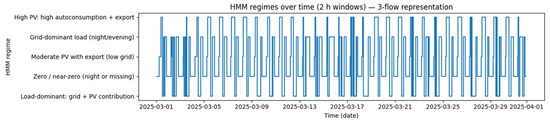
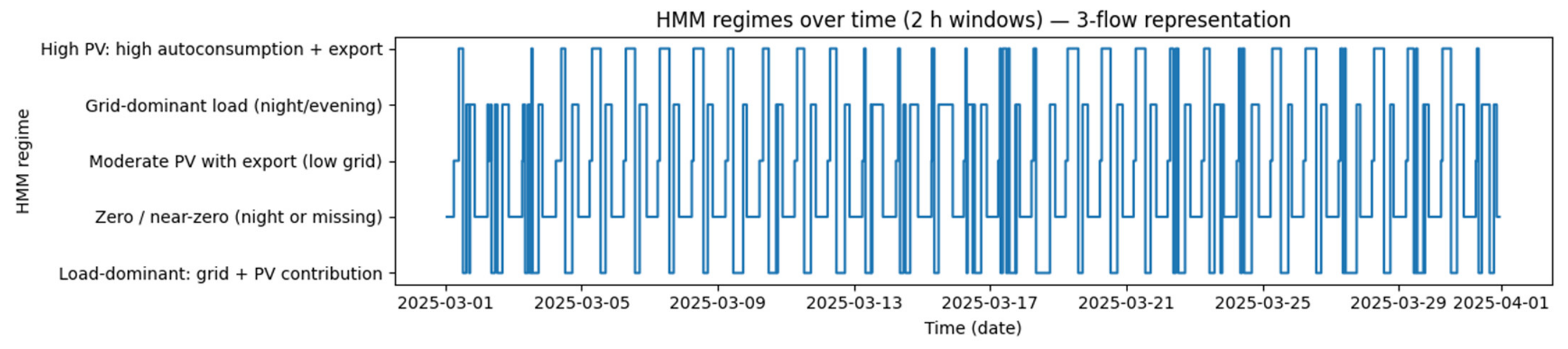
The temporal evolution of the identified energy flow regimes over the entire observation period is shown in Figure 7, revealing persistent operating modes and structured transitions consistent with the diurnal organization of photovoltaic generation and building demand.

Figure 7. Temporal evolution of the energy flow regimes identified by the window-based hidden Markov model, illustrating regime persistence and structured transitions over the entire observation period.

Figure 7 presents the temporal evolution of the energy flow regimes identified by the window-based hidden Markov model over the entire observation period. The results reveal that system operation is dominated by a limited number of persistent regimes, each lasting for extended time intervals rather than appearing as short-lived fluctuations. A pronounced diurnal structure was observed, with photovoltaic-driven regimes occurring predominantly during daylight hours and grid-dominated regimes prevailing during nighttime periods. Transitions between regimes were not random but followed repeatable temporal patterns, indicating physically constrained pathways of system evolution driven by the interaction between photovoltaic generation and building demand. Overall, the figure demonstrates that the PV–building system operates as an organized dynamic process characterized by regime persistence and structured transitions rather than by irregular switching between instantaneous states.

4.4. Regime Persistence and Time-of-Day Structure

The persistence analysis reveal substantial differences in the typical duration of the identified energy flow regimes. Grid-dominated regimes are characterized by long, uninterrupted residence times, reflecting stable nighttime or low-generation operating conditions. In contrast, photovoltaic-driven regimes exhibit shorter but more structured durations, concentrated around periods of significant solar availability.

The time-of-day distribution further confirms a strong diurnal organization of system operation, with distinct regimes systematically associated with specific hours of the day. Autoconsumption-dominated and surplus-export regimes occur predominantly during midday hours, while regimes with high grid dependency dominate during early morning and nighttime periods.

Importantly, intermediate regimes appear consistently during morning ramp-up and evening decline phases, indicating gradual transitions rather than abrupt switching between energetically extreme states. Together, the persistence and time-of-day analyses demonstrate that regime occurrence is governed by repeatable temporal patterns linked to the interaction between photovoltaic generation profiles and building demand. These findings support the interpretation of the PV–building system as a structured dynamic process with temporally organized operating modes.

4.5. Physical Definition of Operating Regimes Based on Energy Balance Constraints

The physical interpretation of the identified HMM regimes was refined using the instantaneous power balance of the monitored PV–building system. Let P_PV(t) denote photovoltaic power generation and P_load(t) denote total building electricity demand at time step t. The three energy flow components used in the analysis are defined as:

$$P_{self}\left(t\right)=min\left(P_{PV}\left(t\right), P_{load}\left(t\right)\right)$$

$$P_{surplus}\left(t\right)=max\left(P_{PV}\left(t\right)-P_{load}\left(t\right),0\right)$$

$$P_{grid}\left(t\right)=max\left(P_{load}\left(t\right)-P_{PV}\left(t\right),0\right)$$

Thus, the operating condition of the PV–building system is governed by the instantaneous power mismatch:

$$∆P\left(t\right)=P_{PV}\left(t\right)-P_{load}\left(t\right)$$

When ΔP(t) < 0, photovoltaic generation is insufficient to cover building demand and the remaining power must be imported from the grid. When ΔP(t) > 0, local demand is saturated, and surplus photovoltaic power is exported to the grid. When ΔP(t) ≈ 0, the system operates close to the balance boundary, and small changes in PV generation or building demand may shift the system between grid import and surplus export. These boundary conditions provide the physical explanation for the occurrence of intermediate transitional regimes.

The HMM regimes can therefore be interpreted not only as statistical states, but also as characteristic regions of the PV–building power balance. Grid-dominated regimes correspond to windows in which P_PV(t) is zero or substantially lower than P_load(t). Photovoltaic-assisted regimes occur when local PV generation contributes to building demand but does not fully eliminate grid import. Self-consumption-dominated and transitional regimes occur near the balance boundary, where both the magnitude and direction of ΔP(t) may vary within the window. Surplus-export regimes occur when photovoltaic generation exceeds the local demand for a substantial part of the window.

Since solar irradiance was not directly measured in the monitoring system, photovoltaic power generation was used as an operational proxy for solar availability. This choice is consistent with the objective of the study, which was to analyze measured electrical energy flows rather than meteorological drivers. Consequently, the physical definition of regimes was based on measured PV production, measured building demand, and the derived energy flow components.

To strengthen the physical interpretation of the HMM states, the identified regimes were characterized using both measured and derived power-flow variables. Table 5 summarizes the typical values of photovoltaic production, self-consumption, surplus export, and grid import for each regime. This quantitative description links the statistically identified hidden states with the underlying PV–building power balance and helps distinguish grid-dominated, transitional, self-consumption, and surplus-export operating conditions.

Table 5. Quantitative characterization of HMM operating regimes based on measured and derived power flows.

Operating Condition	Dominant Balance Condition	PV Production Mean/P95 [kW]	Self-Consumption Mean/P95 [kW]	Surplus Export Mean/P95 [kW]	Grid Import Mean/P95 [kW]	Dominant Time Context
Near-zero/inactive-flow state	PPV ≈ 0, Pload ≈ 0	0.00/0.00	0.00/0.00	0.00/0.00	0.00/0.00	Night/no-flow intervals
Grid-supplied base-load state	PPV = 0, Pgrid ≈ Pload	0.00/0.00	0.00/0.00	0.00/0.00	1.68/7.09	Evening/night
PV-assisted grid-dominant state	0 < PPV < Pload, grid deficit remains	2.59/9.39	2.58/9.39	0.01/0.00	9.18/19.00	Afternoon/evening transition
Low-load daylight transition state	PPV ≈ Pload or mixed sign within window	1.78/5.89	0.69/3.11	0.90/3.95	1.00/6.33	Morning transition
High-PV self-consumption and export state	PPV > Pload for a substantial part of the window	18.14/30.96	15.92/28.83	2.22/7.33	4.56/14.55	Daytime/high PV period

The quantitative characterization confirms that the intermediate states are not arbitrary statistical artifacts. They correspond to windows located near the power-balance boundary between PV-deficit and PV-surplus operation. In these windows, grid import and surplus export may both appear within the same temporal window because PV generation and building demand change continuously over time. This explains why direct transitions between extreme regimes are rare: the system usually passes through balance-boundary states before moving from grid-dominated operation to PV-surplus operation or vice versa.

4.6. Transition Structure Between Regimes

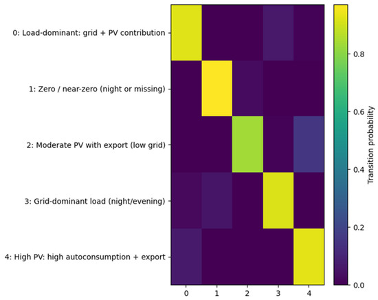
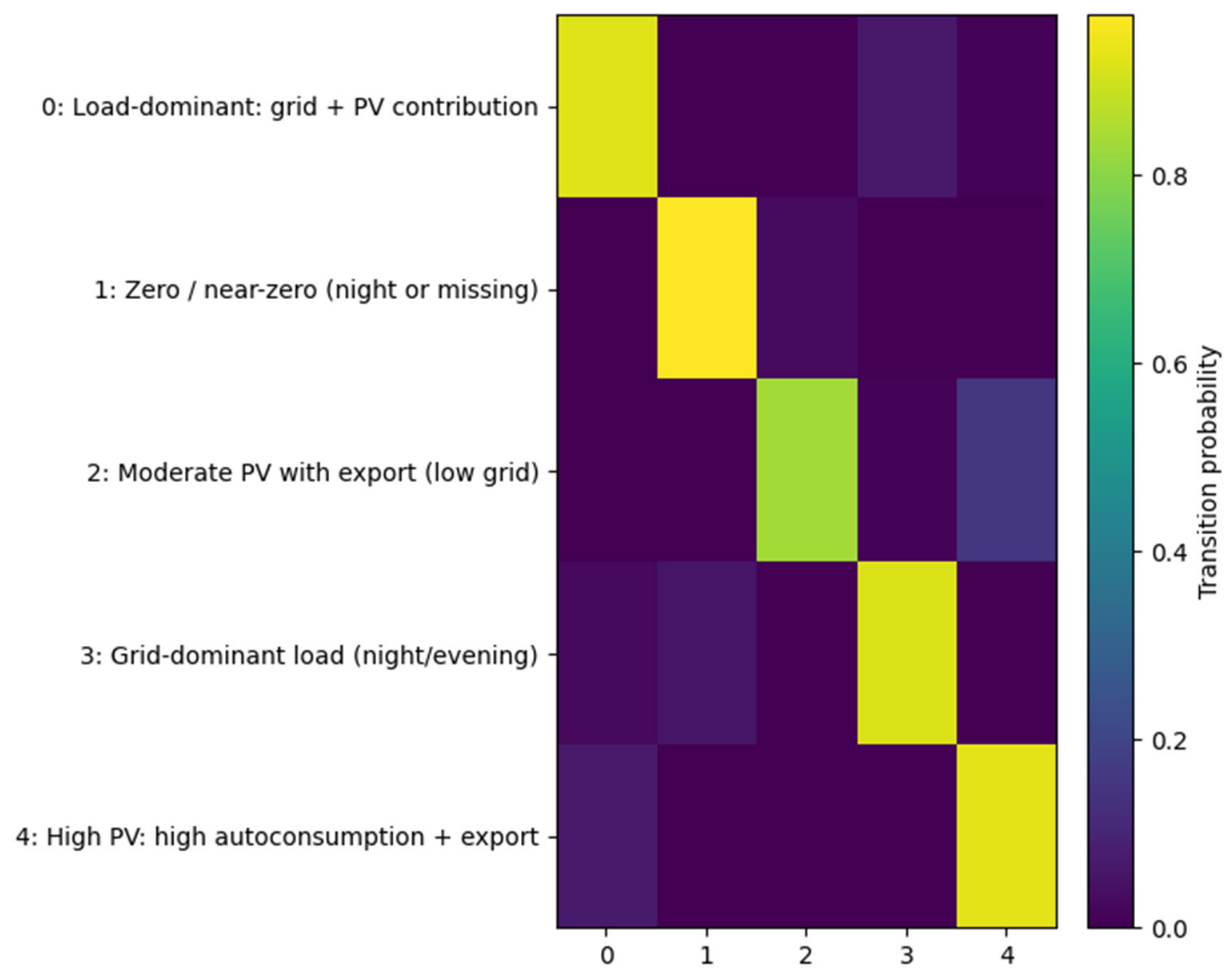
The transition matrix presented in Figure 8 provides a compact representation of the dynamic pathways connecting the identified energy flow regimes. The matrix is characterized by pronounced diagonal dominance, indicating a high probability of remaining in the same regime once entered and confirming the strong persistence observed in the temporal evolution analysis. Off-diagonal elements are unevenly distributed, revealing preferred transition pathways rather than uniform switching between regimes.

Figure 8. HMM transition matrix.

Transitions between photovoltaic-driven and grid-dominated regimes typically occur through intermediate states associated with partial photovoltaic contribution, reflecting the gradual evolution of solar generation and building demand. Direct transitions between energetically extreme regimes are rare, which highlights the presence of physical constraints governing system operation. These constraints arise from the smooth diurnal variation of photovoltaic production and the inertia of building electricity demand, which together limit abrupt changes in energy allocation.

Moreover, the asymmetry of the transition probabilities indicates directional behavior in regime evolution, with morning transitions differing systematically from evening transitions. This directional structure further supports the interpretation of the PV–building system as a non-random dynamic process governed by repeatable daily trajectories. Overall, the transition analysis demonstrates that regime dynamics are structured, constrained, and strongly time-dependent, providing insights that are inaccessible through point-wise regime identification alone.

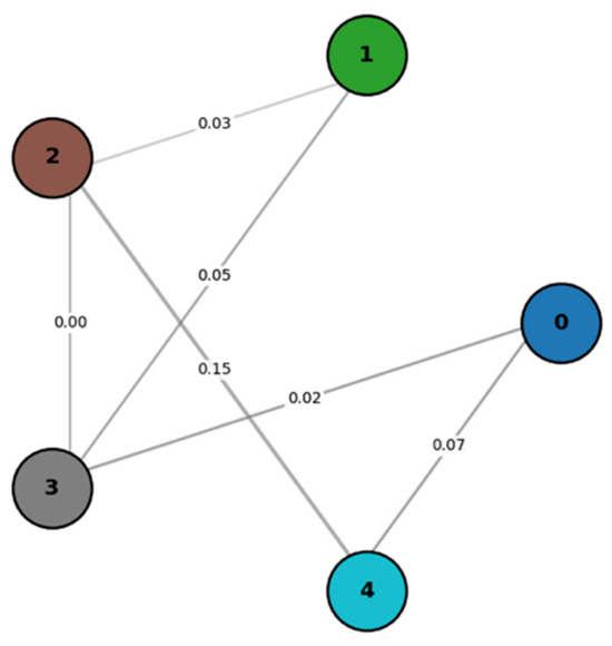
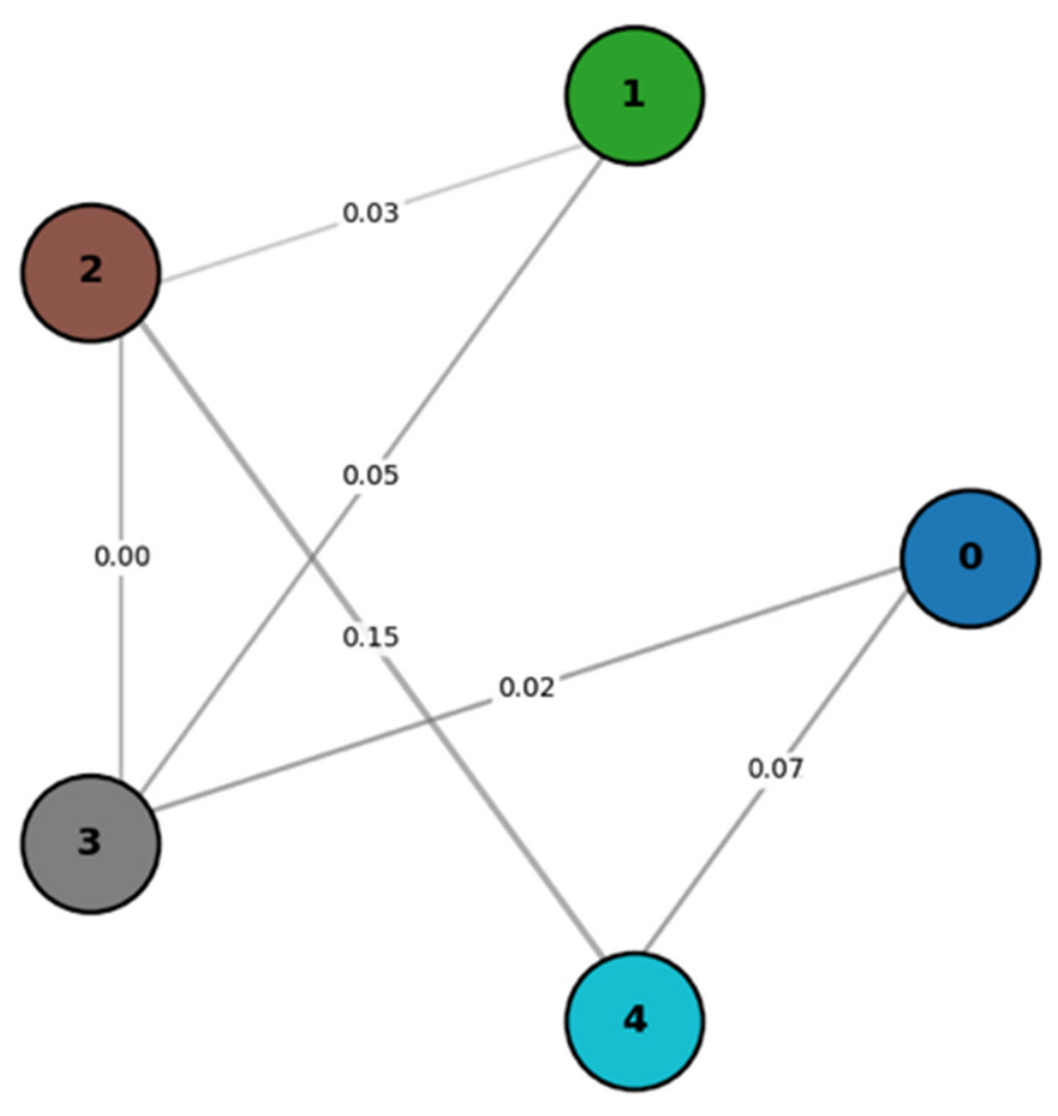
Figure 9 visualizes the complete regime-to-regime transition structure, including both dominant and low-probability transitions. While all transitions are formally possible, their strongly heterogeneous probabilities reveal that system dynamics are governed by a small number of preferred pathways. In contrast to the full transition matrix, the graph emphasizes only statistically and physically relevant transitions, thereby revealing the backbone of regime evolution. The resulting structure is sparse and strongly directional, indicating that the PV–building system follows preferred transition sequences rather than freely switching between all possible regimes.

Figure 9. Directed transition graph illustrating the dominant pathways between energy flow regimes derived from the hidden Markov model transition structure. The numbers shown inside the circles indicate the cluster numbers.

Certain regimes act as transitional hubs, connecting photovoltaic-driven and grid-dominated operating modes, while others appear as terminal or boundary states with limited outgoing transitions. This topology reflects the gradual nature of changes in photovoltaic generation and building demand, which constrain the system to evolve through intermediate operating conditions. Overall, the transition graph reinforces the interpretation of regime dynamics as an organized, path-dependent process shaped by physical energy flow constraints.

In Figure 9, self-transitions corresponding to remaining in the same regime are intentionally not shown. These self-transition probabilities dominate the transition matrix and primarily reflect regime persistence rather than changes in system operation. Omitting self-loops improves the readability of the transition graph and highlights inter-regime transitions that govern the dynamic evolution of the system.

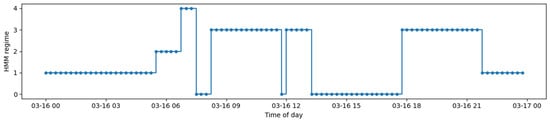
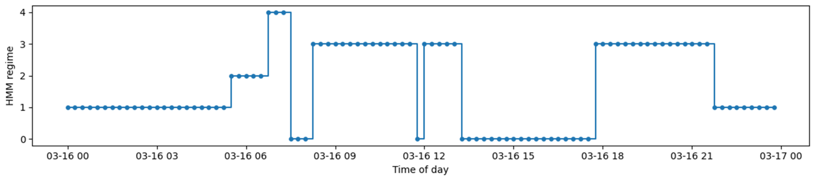
Figure 10 provides a single-day example of regime evolution, illustrating how the transition structure identified by the hidden Markov model manifests in real system operation. The sequence exhibits extended residence times within individual regimes, interrupted by a limited number of transitions occurring at characteristic times of day. This example confirms that regime changes are temporally structured and aligned with the diurnal evolution of photovoltaic generation and building demand.

Figure 10. Regime evolution over a representative day (16 March 2025), shown as a stepwise sequence of hidden Markov model states highlighting regime durations and transition times.

5. Discussion

5.1. From Point-Wise Energy Metrics to Process-Oriented Regime Analysis

Traditional analyses of photovoltaic–building systems are commonly based on point-wise energy metrics, such as instantaneous power values, daily averages, or aggregated energy balances. While such descriptors are useful for assessing overall performance, they fail to capture the temporal organization of system operation and the persistence of characteristic operating conditions. In particular, point-wise representations do not distinguish between short-lived fluctuations and stable operational modes that govern system behavior over meaningful time scales.

The window-based regime analysis proposed in this study addresses these limitations by explicitly incorporating temporal context into the modeling framework. Instead of treating individual measurements as independent observations, system operation is represented as a sequence of short-term behavioral segments, each characterized by its internal dynamics and energy flow structure. This shift enables the identification of persistent operating regimes and reveals the structured nature of regime transitions driven by photovoltaic generation and building demand.

As demonstrated in Section 4, this process-oriented perspective provides insights that are inaccessible through purely static or instantaneous metrics. By focusing on temporal continuity, regime persistence, and transition pathways, the proposed approach captures the dynamic character of energy system operation and offers a more faithful representation of real-world PV–building interactions.

The observed persistence of regimes and structured transitions can be interpreted in the spirit of dynamic systems theory, where stable and unstable states and bifurcations govern the evolution of complex processes [30]. The regime-based representation obtained via HMM can be interpreted as a data-driven analogue of stability and bifurcation structures known from dynamic systems theory, where complex systems exhibit multiple stable states and structured transitions between them.

5.2. Regime Persistence and Characteristic Temporal Scales

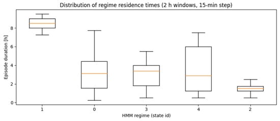
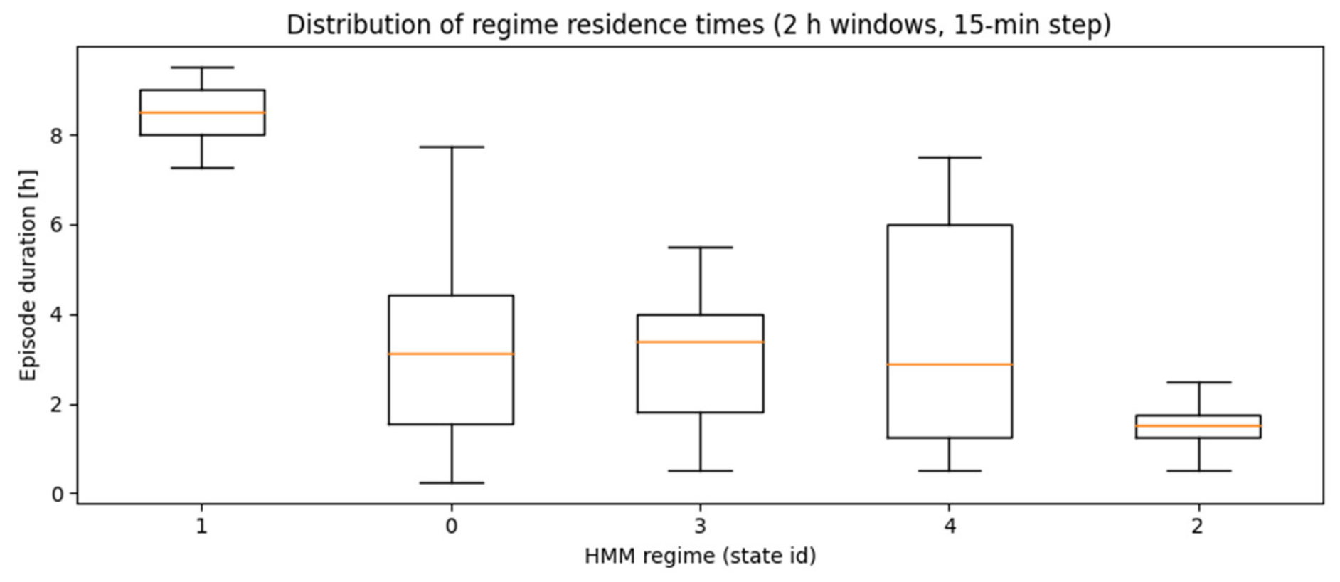
The distribution of regime residence times shown in Figure 11 provides insight into the characteristic temporal scales governing PV–building system operation. Rather than exhibiting uniform or arbitrary durations, the identified regimes display markedly different persistence properties, indicating that each regime corresponds to a distinct and physically meaningful operating mode. In particular, grid-dominated regimes are associated with long residence times, reflecting stable nighttime conditions and limited short-term variability.

Figure 11. Distribution of regime residence times.

In contrast, photovoltaic-driven regimes exhibit shorter but well-defined residence times, typically confined to periods of sustained solar availability. These regimes are interrupted by transitional states occurring during morning ramp-up and evening decline phases, which act as temporal bridges between energetically distinct operating modes. The presence of such intermediate regimes confirms that system evolution is gradual and structured, rather than characterized by abrupt switching.

Importantly, the broad yet bounded distributions of residence times suggest that regime persistence is governed by underlying physical processes rather than by artifacts of segmentation or window length. The observed temporal scales are consistent with the diurnal dynamics of photovoltaic generation and building demand, reinforcing the interpretation of regimes as quasi-stationary states of system operation. Overall, the residence time analysis demonstrates that incorporating temporal persistence is essential for understanding energy system behavior beyond instantaneous power metrics.

5.3. Structured Regime Transitions and Constrained System Dynamics

The transition structure identified by the hidden Markov model reveals that regime changes in the PV–building system are highly organized and constrained. As illustrated by the transition matrix (Figure 7) and its graph-based representation (Figure 8), regime evolution is dominated by a limited number of preferred pathways rather than by uniform switching between all possible operating modes. This structure indicates that transitions are governed by physical and operational constraints imposed by photovoltaic generation profiles and building electricity demand.

The strong diagonal dominance of the transition matrix reflects high regime persistence, while the heterogeneous off-diagonal probabilities reveal directional and asymmetric transition behavior. In particular, transitions between photovoltaic-driven and grid-dominated regimes typically occur through intermediate operating states, as further illustrated by the single-day example shown in Figure 10. Direct transitions between energetically extreme regimes are rare, highlighting the gradual nature of system evolution.

Taken together, these findings demonstrate that the PV–building system behaves as a constrained dynamic process characterized by repeatable trajectories in regime space. The observed transition structure cannot be captured by static representations or point-wise analyses, underscoring the importance of modeling temporal continuity and transition pathways when analyzing integrated energy systems.

An important complementarity emerges when Figure 8 and Figure 11 are considered jointly. While the transition graph (Figure 8) quantifies the probabilities of switching from one regime to another, the distribution of regime residence times (Figure 11) reveals how long the system typically remains within each regime before such transitions occur. High self-persistence and long residence times correspond to low overall transition probabilities, whereas regimes characterized by shorter residence times exhibit higher likelihoods of transitioning to neighboring states. Together, these figures demonstrate that regime dynamics are governed not only by the probability of transitions, but also by the temporal scales over which transitions can realistically occur.

The refined physical interpretation shows that directional transitions arise from the evolution of the power mismatch ΔP(t) = P_PV(t) − P_load(t). During morning ramp-up, ΔP(t) typically moves from negative values toward zero and then positive values, causing the system to pass from grid-dominated operation through intermediate self-consumption states toward PV-driven regimes. During evening decline, the reverse process occurs as photovoltaic generation decreases while building demand may remain positive. This explains the observed transition asymmetry without requiring additional assumptions beyond the measured power balance.

5.4. Quantitative Comparison with Previous Methods Applied to the Same Dataset

The proposed window-based HMM framework was evaluated not as an isolated algorithmic transfer, but as a continuation of previous data-driven analyses performed by the authors on the same PV–building dataset. The same monitored system—a 50 kWp photovoltaic installation supplying the administrative building of WSEI University in Lublin—was previously analyzed using unsupervised clustering and dynamic time warping. This enables a direct methodological comparison without introducing differences caused by another building, another season, or another measurement system.

Previous clustering-based studies identified power signatures and operating states from 15 min measurement data. In these approaches, individual observations were treated as independent points in a production–consumption or energy-flow state space. This allowed for the identification of characteristic operating conditions, such as high self-consumption, surplus export, and grid-import-dominated operation. The usefulness of this approach lies in its simplicity, interpretability, and ability to quantify the frequency of operating states. However, clustering does not inherently model the temporal continuity of operation, because each observation is classified independently of the preceding and following time steps.

A second methodological layer was introduced using dynamic time warping. DTW was applied to daily PV generation and building demand profiles in order to quantify temporal mismatch and similarity between days. This approach revealed that days with similar energy states may still differ substantially in their temporal organization. Quantitatively, DTW distance was significantly related to the temporal overlap between PV generation and building load, with a Pearson correlation r = −0.60 and Spearman correlation ρ = −0.53, confirming that temporal mismatch constitutes an operationally meaningful dimension of PV–building interaction. Nevertheless, DTW operates at the level of daily profile similarity and does not identify within-day latent operating regimes or transition probabilities between them.

The present window-based HMM framework adds a third analytical layer. Instead of treating observations as independent points or comparing entire daily profiles, the method represents system operation as a sequence of short temporal windows. Each window summarizes local energy-flow behavior, and the HMM identifies latent regimes together with their persistence and transition probabilities. This enables the direct quantification of regime residence times, self-transition probabilities, and preferred transition pathways. These quantities are essential for process-oriented interpretation and cannot be obtained directly from static clustering or DTW alone.

To clarify the methodological contribution of the proposed approach, the window-based HMM framework was compared with methods previously applied by the authors to the same March 2025 PV–building dataset. Table 6 summarizes the main analytical objectives, data representations, outputs, and limitations of these approaches. The comparison highlights that the proposed HMM framework does not replace earlier clustering- or DTW-based analyses, but extends them by adding an explicit probabilistic description of regime persistence and transition dynamics.

Table 6. Comparison of previously applied methods and the proposed window-based HMM framework for the March 2025 PV–building dataset.

Method	Main Analytical Object	Main Output	Temporal Continuity	Transition Dynamics	Main Limitation
Point-wise k-means clustering [21]	Independent 15 min observations	Power signatures, operating states, cluster frequencies	Not modeled directly	Reconstructed only post hoc	Treats observations as independent
Energy-flow clustering [31]	Autoconsumption, surplus, grid import	Physically interpretable flow regimes	Limited	Deterministic transition counts	No probabilistic regime dynamics
DTW-based analysis [22]	Daily PV and load profiles	Temporal mismatch, profile similarity, representative/extreme days	Captured at daily profile level	No intra-day transition matrix	Does not identify persistent latent regimes
Window-based HMM	Sliding-window energy-flow features	Latent regimes, transition matrix, residence times	Explicitly modeled	Probabilistic and directional	Requires parameter sensitivity and interpretability assessment

The comparison shows that the proposed method does not duplicate the information provided by previous approaches. Instead, it complements them by addressing a different analytical question. Clustering answers the question: which operating states occur? DTW answers the question: how similar or mismatched are the daily PV and load profiles? The window-based HMM answers the question: how does the PV–building system move between persistent operating regimes over short time horizons?

This distinction is important from the perspective of energy management. Static clustering is useful for identifying operating categories, while DTW is useful for diagnosing temporal mismatch between daily profiles. However, operational control requires knowledge of whether the system is likely to remain in the current regime or transition toward another one. The HMM transition matrix and residence-time distributions provide this missing information, making the proposed framework more suitable for process-oriented monitoring and future control-oriented applications.

The proposed method is not intended to replace clustering or DTW, but to extend the authors’ previous analyses by adding a probabilistic, process-oriented layer that quantifies regime persistence and directional transition pathways.

5.5. Implications for Energy System Analysis and Monitoring

Several limitations of the proposed regime-based analysis should be acknowledged. First, the results depend on the choice of window length and overlap, which influence the balance between temporal resolution and regime stability. Second, the number of regimes specified in the hidden Markov model affects the granularity of the identified operating modes and may require adjustment when analyzing systems with different sizes or usage patterns. Additionally, the selection of features used to characterize each window can impact regime separability and interpretability.

Future research may address these limitations by exploring adaptive or multi-scale windowing strategies that capture both short-term fluctuations and long-term operational trends. The integration of regime analysis across multiple buildings or seasons would enable comparative studies and support generalization of the proposed framework. Furthermore, coupling regime identification with control or forecasting applications could provide practical benefits for energy management and the monitoring of photovoltaic–building systems.

5.6. Limitations and Directions for Future Research

The proposed regime-based framework involves several methodological choices that influenced the obtained results. In particular, the length of the sliding window and the predefined number of regimes affect the temporal resolution and the level of detail of the identified operating modes. While the selected parameters were found to provide a stable and interpretable representation for the analyzed dataset, different systems or usage patterns may require re-tuning of these settings.

Future work should therefore investigate adaptive and multi-scale approaches that allow regime identification across multiple temporal horizons. Extending the analysis to longer observation periods, different seasons, or multiple buildings would enable an assessment of the robustness and generalizability of the proposed methodology. In addition, integrating regime-based analysis with monitoring, anomaly detection, or control strategies represents a promising direction for practical applications in energy system management.

6. Conclusions

This study presented a window-based analytical pipeline for identifying and interpreting operating regimes and their dynamics in a photovoltaic–building energy system. By combining energy flow decomposition with temporal windowing and hidden Markov modeling, the proposed approach captures regime persistence, characteristic temporal scales, and structured transition pathways that are not accessible through point-wise or static analyses. The results demonstrate that system operation is dominated by a limited number of stable regimes organized according to a clear diurnal structure.

The analysis of regime transitions revealed constrained and directional dynamics, with transitions occurring preferentially through intermediate operating states rather than via abrupt switching between energetically extreme conditions. Furthermore, the distribution of regime residence times confirmed that individual regimes exhibit distinct and physically meaningful temporal scales, reinforcing their interpretation as quasi-stationary operating modes.

The proposed regime-based framework provides a process-oriented perspective on PV–building system operation, offering enhanced interpretability of temporal behavior and system dynamics. The approach is broadly applicable to high-resolution energy datasets and can support improved monitoring and the analysis of integrated energy systems.

The comparison with previously applied methods confirms that the proposed HMM framework should be interpreted as an additional analytical layer rather than a replacement for clustering or DTW. Static clustering provides physically interpretable operating states but does not model temporal continuity. DTW captures daily temporal mismatch but does not segment intra-day operation into persistent regimes. The window-based HMM combines the advantages of both perspectives by preserving short-term temporal context and providing a probabilistic transition structure. Therefore, the core contribution of this study is not the introduction of HMM as a new algorithm, but its integration into a physically interpretable energy-flow framework for quantifying regime persistence and transition dynamics in PV–building systems.

References

- Ahmed, S.; Ali, A.; Qadir, S.A.; Ramunno, D.; D’Angola, A. Modelling of Energy Management Strategies in a PV-Based Renewable Energy Community with Electric Vehicles. World Electr. Veh. J. 2025, 16, 302. [Google Scholar] [CrossRef] [Scilit]
- Singh, A.; Shankar, R.; Kumar, A. A Comprehensive Review of Load Frequency Control and Solar Energy Integration: Challenges & Opportunities in Indian Context. Energies 2025, 18, 843. [Google Scholar] [CrossRef] [Scilit]
- Walichnowska, P.; Kruszelnicka, W.; Tomporowski, A.; Mroziński, A. The Impact of Energy Storage on the Efficiency of Photovoltaic Systems and Determining the Carbon Footprint of Households with Different Electricity Sources. Sustainability 2025, 17, 2765. [Google Scholar] [CrossRef] [Scilit]
- García-Guillén, A.; Gutiérrez-Hinestroza, M.; Moreno-Alcívar, L.; Bravo-Montero, L.; Herrera-Franco, G. Photovoltaic System for Residential Energy Sustainability in Santa Elena, Ecuador. Environments 2025, 12, 281. [Google Scholar] [CrossRef] [Scilit]
- Khandelwal, A.K.; Tsoukalas, C.A.; Zhao, Y.; Ishii, M. Objective Neural Network-Based Flow Regime Classifiers with Application to Vertical, Narrow, Rectangular Channels and Round Pipe Geometry. J. Nucl. Eng. 2026, 7, 15. [Google Scholar] [CrossRef] [Scilit]
- Yan, H.; Zhang, C.; Li, W.; Chen, N. A Study on the Evolution of Flow Regime in a Gas-Assisted Submerged High-Pressure Water Jet. Fluids 2026, 11, 15. [Google Scholar] [CrossRef] [Scilit]
- Uysal, E.; Durak, G.; Kotek Sedef, A.; Bagci, U.; Berber, T.; Gurdal, N.; Akkus Yildirim, B. Unsupervised Clustering Successfully Predicts Prognosis in NSCLC Brain Metastasis Cohorts. Diagnostics 2025, 15, 1747. [Google Scholar] [CrossRef] [Scilit] [PubMed]
- Correia, C.; Paredes, S.; Rocha, T.; Henriques, J.; Bernardino, J. Benchmarking Methods for Pointwise Reliability. Information 2025, 16, 327. [Google Scholar] [CrossRef] [Scilit]
- Lin, X.; Niu, Y.; Yan, Z.; Zou, L.; Tang, P.; Song, J. Hybrid Photovoltaic Output Forecasting Model with Temporal Convolutional Network Using Maximal Information Coefficient and White Shark Optimizer. Sustainability 2024, 16, 6102. [Google Scholar] [CrossRef] [Scilit]
- Pérez-Martínez, M.; Barranco-Merino, R.; Higuera-Trujillo, J.L.; Llinares, C. Temporal Trajectories in EEG-Based Mental Workload: Effects of Workspace Type. Buildings 2026, 16, 176. [Google Scholar] [CrossRef] [Scilit]
- Unggul, D.B.; Iriawan, N.; Irhamah, I. Parameter Estimation of MSNBurr-Based Hidden Markov Model: A Simulation Study. Symmetry 2025, 17, 1931. [Google Scholar] [CrossRef] [Scilit]
- Tampouris, A.; Dritsaki, C. Adaptive Hierarchical Hidden Markov Models for Structural Market Change. J. Risk Financ. Manag. 2026, 19, 15. [Google Scholar] [CrossRef] [Scilit]
- Nguyen, N.; Nguyen, D. Global Stock Selection with Hidden Markov Model. Risks 2021, 9, 9. [Google Scholar] [CrossRef] [Scilit]
- Borucka, A.; Kozłowski, E.; Parczewski, R.; Antosz, K.; Gil, L.; Pieniak, D. Supply Sequence Modelling Using Hidden Markov Models. Appl. Sci. 2023, 13, 231. [Google Scholar] [CrossRef] [Scilit]
- Zeng, Z.; Qin, J.; Wu, T. A Knowledge Graph-Enhanced Hidden Markov Model for Personalized Travel Routing: Integrating Spatial and Semantic Data in Urban Environments. Smart Cities 2025, 8, 75. [Google Scholar] [CrossRef] [Scilit]
- Unggul, D.B.; Iriawan, N.; Irhamah, I.; Prabowo, A.A. SEP-HMM: A Flexible Hidden Markov Model Framework for Asymmetric and Non-Mesokurtic Emission Patterns. Mathematics 2026, 14, 393. [Google Scholar] [CrossRef] [Scilit]
- Yang, R.; Tang, J.; Saga, R.; Ma, Z. A Dynamic Hidden Markov Model with Real-Time Updates for Multi-Risk Meteorological Forecasting in Offshore Wind Power. Sustainability 2025, 17, 3606. [Google Scholar] [CrossRef] [Scilit]
- Rimella, L.; Whiteley, N. Hidden Markov Neural Networks. Entropy 2025, 27, 168. [Google Scholar] [CrossRef] [Scilit] [PubMed]
- Lin, L.; You, Z.; Li, F.; Liu, J.; Yang, C. A Two-Stage Hidden Markov Model for Medium- to Long-Term Multiple Wind Farm Power Scenario Generation. Energies 2025, 18, 1917. [Google Scholar] [CrossRef] [Scilit]
- Hopwood, M.W.; Patel, L.; Gunda, T. Classification of Photovoltaic Failures with Hidden Markov Modeling, an Unsupervised Statistical Approach. Energies 2022, 15, 5104. [Google Scholar] [CrossRef] [Scilit]
- Małek, A.; Caban, J.; Gryniewicz-Jaworska, M.; Marciniak, A.; Bednarczyk, T. A Method for Assessing the Selection of a Photovoltaic System for a Building’s Energy Needs Based on Unsupervised Clustering. Appl. Sci. 2025, 15, 9062. [Google Scholar] [CrossRef] [Scilit]
- Małek, A.; Piotrowska, K.; Gryniewicz-Jaworska, M.; Marciniak, A. Time-Resolved Analysis of Photovoltaic–Building Energy Matching Using Dynamic Time Warping. Energies 2026, 19, 1107. [Google Scholar] [CrossRef] [Scilit]
- Małek, A.; Caban, J.; Vrábel, J.; Marciniak, A. Combining State-Based Clustering and Dynamic Time Warping for the Analysis of Photovoltaic–Building Energy Interactions. Energies 2026, 19, 838. [Google Scholar] [CrossRef] [Scilit]
- Azevedo, I.; Leal, V. Decomposition Analysis of the Evolution of the Local Energy System as a Tool to Assess the Effect of Local Actions: Methodology and Example of Malmö, Sweden. Energies 2021, 14, 461. [Google Scholar] [CrossRef] [Scilit]
- Jin, Y.; Shen, W.; Wu, C.Q. Power Prediction Based on Signal Decomposition and Differentiated Processing with Multi-Level Features. Electronics 2025, 14, 2036. [Google Scholar] [CrossRef] [Scilit]
- Wang, F.-C.; Huang, H.-T. Extended-Window Algorithms for Model Prediction Applied to Hybrid Power Systems. Technologies 2024, 12, 6. [Google Scholar] [CrossRef] [Scilit]
- Prajapati, J.I.; Das, R. Sliding Window-Based Randomized K-Fold Dynamic ANN for Next-Day Stock Trend Forecasting. Computation 2025, 13, 141. [Google Scholar] [CrossRef] [Scilit]
- Rastogi, A.K.; Taterh, S.; Kumar, B.S. Dimensionality Reduction Algorithms in Machine Learning: A Theoretical and Experimental Comparison. Eng. Proc. 2023, 59, 82. [Google Scholar] [CrossRef] [Scilit]
- Sun, T.; He, L.; Fang, X.; Xie, L. Enhanced Multilinear PCA for Efficient Image Analysis and Dimensionality Reduction: Unlocking the Potential of Complex Image Data. Mathematics 2025, 13, 531. [Google Scholar] [CrossRef] [Scilit]
- Cygan, S.; Marciniak-Czochra, A.; Münnich, F.; Oelz, D. Stability and bifurcation analysis in a mechanochemical model of pattern formation. arXiv 2026, arXiv:2602.09998. [Google Scholar]
- Marciniak, A.; Małek, A. Determining Energy Production and Consumption Signatures Using Unsupervised Clustering. Energies 2025, 18, 2571. [Google Scholar] [CrossRef] [Scilit]
Disclaimer/Publisher’s Note: The statements, opinions and data contained in all publications are solely those of the individual author(s) and contributor(s) and not of MDPI and/or the editor(s). MDPI and/or the editor(s) disclaim responsibility for any injury to people or property resulting from any ideas, methods, instructions or products referred to in the content. |
© 2026 by the authors. Licensee MDPI, Basel, Switzerland. This article is an open access article distributed under the terms and conditions of the Creative Commons Attribution (CC BY) license.