A Regime-Adaptive Imbibition Model for Fracturing-Fluid Species Transport in Ultra-Low-Permeability Gas Reservoirs

Abstract

Hydraulic fracturing creates long-lasting contact between aqueous fracturing fluids and gas-bearing ultra-low permeability matrix rock, making fluid retention and dissolved-species penetration important for interpreting matrix–fracture mass exchange and post-fracturing flowback behavior. These processes are controlled by the coupled effects of capillary imbibition, fracture–matrix pressure assistance, and species diffusion, but their relative importance is difficult to distinguish through a concentration profile. This study develops a regime-adaptive pressure-assisted imbibition and species-transport framework for interpreting fracturing-fluid species movement from a hydraulic fracture into a gas-bearing porous matrix. The framework couples a pressure-assisted imbibition (PAI) model with a one-dimensional advection–diffusion equation (ADE), where the PAI-derived velocity provides the transient advective input for species transport. The same formulation continuously represents capillary-dominated, mixed pressure–capillary, and pressure-dominated behavior without switching governing equations. Three diagnostic limiting cases, Capillary-driven Advection, Pressure-driven Advection, and Diffusion-only, are introduced to compare reduced mechanism-specific responses with the Full PAI-ADE response without interpreting them as additive components of the full solution. At 100 days, the Full PAI-ADE concentration front in the Ultra-Low Matrix reached 31.9 cm at $C=0.10$, compared with 18.0 cm for Capillary-driven Advection, 9.2 cm for Pressure-driven Advection, and 21.7 cm for Diffusion-only, indicating a mixed diffusion–capillary response. For the High-Perm Matrix at 0.20 day, the Full PAI-ADE and Pressure-driven Advection fronts reached 211.6 and 210.9 cm, respectively, with a normalized profile error of 0.003, identifying a pressure-advection-dominated limiting behavior. A dimensionless mechanism-weight analysis based on the pressure–capillary ratio (${\mathsf{\Pi }}_{\mathrm{p}\mathrm{c}}$) and front-scale Péclet number (Pe) further summarizes these behaviors. The results demonstrate that the proposed framework provides a compact diagnostic tool for linking pressure–capillary driving, advective–diffusive tendency, and observable species-transport profiles in ultra-low permeability gas-reservoir applications.

1. Introduction

Hydraulic fracturing is widely used to improve hydrocarbon production from tight and shale gas reservoirs by creating conductive fracture networks that connect the wellbore to the low-permeability matrix. During fracturing operations, water-based fracturing fluids containing chemical additives or dissolved species are injected into hydraulic fractures and may remain in contact with gas-bearing matrix rock after pumping [1,2]. A large fraction of the injected fluid may not immediately return during flowback, and in field applications, near-fracture fluid invasion may manifest as prolonged fluid retention, water blocking, delayed or reduced flowback, matrix–fracture mass exchange, and transport of dissolved additives into the contacted matrix region [2,3,4,5,6]. The extent and rate of this fluid uptake depend on matrix properties, pore structure, wettability, initial saturation, and rock–fluid interactions [5,6,7,8]. Contact between the fracturing fluid and shale matrix may also initiate coupled species transport and chemical interactions within the near-fracture region [9,10]. Therefore, understanding fracturing-fluid species penetration from a hydraulic fracture into a gas-bearing matrix is important for interpreting fluid retention, chemical exposure, matrix–fracture mass exchange, and post-fracturing flowback response.

Capillary imbibition is commonly interpreted using Lucas–Washburn-type models and their porous-media extensions [11,12,13,14,15]. These models provide a useful basis for relating interfacial tension, contact angle, pore size, permeability, tortuosity, and viscosity to wetting-phase advancement. However, matrix invasion in hydraulically fractured gas-bearing formations is not necessarily controlled by spontaneous capillary imbibition alone. Previous studies have shown that shale–fluid interaction, salt diffusion, osmotic effects, water adsorption, clay-related effects, and pore-scale heterogeneity can all influence imbibition behavior in shale and tight rocks [8,16,17,18]. Reservoir stimulation may also alter the rock structure and the associated transport pathways. Recent studies of cyclic thermal treatment in granite have reported enhanced microcrack development, increased crack connectivity, and progressive changes in fracture morphology and surface characteristics [19,20]. Temperature variations may also modify wettability and capillary-pressure behavior in subsurface multiphase systems [21]. In addition, pressure gradients imposed during fracturing, shut-in, or pressure redistribution can shift the process from spontaneous imbibition toward forced or mixed imbibition, where capillary and viscous or pressure-driven effects compete [22,23]. Related studies on forced imbibition and heterogeneous porous media have used dimensionless numbers and regime maps to distinguish capillary-dominated and viscous-dominated displacement behavior [24,25]. For dissolved species, transport is further complicated by the coexistence of advection associated with wetting-phase movement and effective diffusion within the contacted matrix region [26,27,28,29]. Although full gas–water two-phase, other subsurface multiphase, or reactive-transport simulations can represent more detailed saturation, pressure, thermal, and chemical processes [30], they require additional constitutive relationships and may obscure the role of individual reduced mechanisms. Therefore, the key research is not only predicting penetration depth or concentration profiles but also identifying whether the observed species-transport response is primarily controlled by capillary-driven advection, pressure-driven advection, diffusion, or a mixed regime.

This study develops a regime-adaptive coupling framework that links a pressure-assisted imbibition (PAI) model with an advection–diffusion equation (ADE) to interpret fracturing-fluid species movement from a hydraulic fracture into a gas-bearing porous matrix. In this framework, the PAI model provides the transient imbibition-front position and advective velocity, while the ADE describes species transport under the combined effects of PAI-derived advection and effective diffusion. Three diagnostic limiting cases, Capillary-driven Advection, Pressure-driven Advection, and Diffusion-only, are introduced to compare the effect of each mechanism. A dimensionless mechanism-weight pattern based on the pressure–capillary ratio (${\mathsf{\Pi }}_{\mathrm{p}\mathrm{c}}$) and front-scale Péclet number (Pe) is then used to summarize these observations. A compact mechanism-oriented diagnostic structure is introduced that links pressure–capillary driving, advective–diffusive transport tendency, and observable concentration profiles without switching governing equations among capillary-dominated, mixed, and pressure-dominated regimes. The paper is organized as follows. Section 2 defines the physical problem, PAI model, species-transport equation, and normalized mechanism weights. Section 3 describes the numerical implementation and computational workflow. Section 4 presents PAI verification, coupled PAI-ADE transport, mechanism-decomposition profiles, and dimensionless mechanism-weight analysis. Section 5 summarizes the main conclusions.

2. Mathematical Modeling

2.1. Physical Problem

The physical problem considered in this study is one-dimensional penetration of an aqueous fracturing fluid from a hydraulic fracture into a gas-bearing porous matrix. The gas-bearing matrix is assumed to be initially partially water-saturated, with a connected resident aqueous phase providing pathways for dissolved-species transport. The resident gas forms the non-wetting background, while the injected aqueous phase provides additional wetting-phase invasion from the fracture face. Accordingly, the PAI front $X\left(t\right)$ represents the characteristic advancement of the invading wetting phase rather than a mathematically sharp boundary separating a fully wetted region from a completely dry region. Wetting-phase movement is driven by capillary suction and may also be assisted by a fracture–matrix pressure difference. The gas–water system is represented through a moving-front idealization rather than through a saturation-resolved two-phase displacement model. The formulation therefore tracks the characteristic wetting-front position and velocity without resolving the complete gas–water saturation distribution. Species transport is then governed by the combined effects of PAI-derived advection and effective diffusion. The matrix is represented as a homogeneous one-dimensional domain of length $L$, with coordinate $x$ measured from the fracture face into the matrix. The normalized concentration is denoted by ($C$). The fracture face is assigned a prescribed concentration ($C_{\mathrm{f}\mathrm{a}\mathrm{c}\mathrm{e}}$), and the matrix is initially solute-free with ($C_{\mathrm{i}\mathrm{n}\mathrm{i}\mathrm{t}\mathrm{i}\mathrm{a}\mathrm{l}}$). The matrix boundary uses a zero-gradient concentration condition.

2.2. Pressure-Assisted Imbibition Model

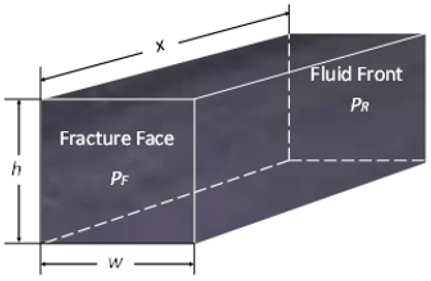
The PAI formulation is introduced to represent capillary-only, mixed pressure–capillary, and pressure-dominated imbibition within a single reduced-order model and to provide a closed-form transient front position and velocity for the subsequent mechanism analysis. The PAI model estimates the imbibition-front position $X\left(t\right)$ by combining capillary and externally imposed pressure driving. The physical configuration and principal variables of the one-dimensional pressure-assisted imbibition model are illustrated in Figure A1. As derived in Appendix A, the PAI solution can be written as Equation (1), where $a$ is the PAI coefficient defined in Equation (2).

$$X\left(t\right)=\sqrt{a t}$$

(1)

$$a={\displaystyle \frac{4 k k_{rw}\left[\sigma cos\left(\theta \right)+0.5 r_c ∆P\right]}{{\mu }_w{ r}_c}}$$

(2)

where $\sigma$ is interfacial tension, $\theta$ is contact angle, $r_c$ is the equivalent pore radius and $∆P=(P_F-P_R)$ is the pressure difference between the fracture and matrix pressure, $k$ is absolute permeability, and ${ \mu }_w$ is wetting-fluid viscosity. The PAI formulation adopts a sharp-front representation in which the wetting-phase saturation at the advancing front, $S_{wf}$, is treated as a prescribed characteristic value. Accordingly, $k_{rw}=k_{rw}\left(S_{wf}\right)$ is constant for a given matrix case. This treatment is consistent with the type of front idealization used in classical Buckley–Leverett descriptions, and the present model therefore predicts the wetting-front position and velocity rather than the complete gas–water saturation profile. The fracture and reservoir pressures, $P_F$ and $P_R$, are prescribed throughout each simulation. The PAI initial conditions are $X\left(0\right)=0$ and $\mathrm{d}X/\mathrm{d}t{\mid }_{t=0} =0$, as detailed in Appendix A.

The capillary-driving and pressure-driving terms are defined in Equations (3) and (4), respectively. The combined driving term is then given by Equation (5).

$$S_{\mathrm{c}\mathrm{a}\mathrm{p}\mathrm{i}\mathrm{l}\mathrm{l}\mathrm{a}\mathrm{r}\mathrm{y}}=\sigma cos\left(\theta \right)$$

(3)

$$S_{\mathrm{p}\mathrm{r}\mathrm{e}\mathrm{s}\mathrm{s}\mathrm{u}\mathrm{r}\mathrm{e}}=0.5 r_c ∆P$$

(4)

$$S_{\mathrm{t}\mathrm{o}\mathrm{t}\mathrm{a}\mathrm{l}}=S_{\mathrm{c}\mathrm{a}\mathrm{p}\mathrm{i}\mathrm{l}\mathrm{l}\mathrm{a}\mathrm{r}\mathrm{y}}+S_{\mathrm{p}\mathrm{r}\mathrm{e}\mathrm{s}\mathrm{s}\mathrm{u}\mathrm{r}\mathrm{e}}$$

(5)

The pressure–capillary ratio, ${\mathsf{\Pi }}_{\mathrm{p}\mathrm{c}}$, is defined in Equation (6) as the ratio of pressure driving to capillary driving. Small ${\mathsf{\Pi }}_{\mathrm{p}\mathrm{c}}$ indicates capillary-dominated PAI driving, while larger ${\mathsf{\Pi }}_{\mathrm{p}\mathrm{c}}$ indicates a stronger pressure-driven component. In this framework, ${\mathsf{\Pi }}_{\mathrm{p}\mathrm{c}}$ is fixed for a given porous-medium model and fixed fluid/pressure condition because $S_{\mathrm{c}\mathrm{a}\mathrm{p}\mathrm{i}\mathrm{l}\mathrm{l}\mathrm{a}\mathrm{r}\mathrm{y}}$ and $S_{\mathrm{p}\mathrm{r}\mathrm{e}\mathrm{s}\mathrm{s}\mathrm{u}\mathrm{r}\mathrm{e}}$ are not time-dependent.

$${\mathsf{\Pi }}_{\mathrm{p}\mathrm{c}}={\displaystyle \frac{S_{\mathrm{p}\mathrm{r}\mathrm{e}\mathrm{s}\mathrm{s}\mathrm{u}\mathrm{r}\mathrm{e}}}{S_{\mathrm{c}\mathrm{a}\mathrm{p}\mathrm{i}\mathrm{l}\mathrm{l}\mathrm{a}\mathrm{r}\mathrm{y}}}}$$

(6)

Using these definitions, the PAI coefficient can be rewritten as Equation (7). The corresponding PAI-derived velocity is given by Equation (8). The analytical solution represents the post-start-up, viscous-dominated response of the full transient PAI equation. As quantified in Appendix A, the inertial relaxation times are many orders of magnitude shorter than the positive times considered in this study. Because the analytical velocity is singular at $t=0$, all transport calculations are evaluated at positive time levels.

$$a={\displaystyle \frac{4 k k_{rw}}{{\mu }_w{ r}_c}}\left[S_{\mathrm{c}\mathrm{a}\mathrm{p}\mathrm{i}\mathrm{l}\mathrm{l}\mathrm{a}\mathrm{r}\mathrm{y}}+S_{\mathrm{p}\mathrm{r}\mathrm{e}\mathrm{s}\mathrm{s}\mathrm{u}\mathrm{r}\mathrm{e}}\right]$$

(7)

$$v\left(t\right)=0.5\sqrt{a/t}$$

(8)

2.3. Species Transport Equation

Species transport is described by a one-dimensional ADE driven by the PAI-derived velocity, as shown in Equation (9). Here, $C(x,t)$ is normalized concentration, $v\left(t\right)$ is the PAI-derived time-dependent advective velocity, and $D_{\mathrm{e}\mathrm{f}\mathrm{f}}$ is the effective diffusion coefficient. The fracture face is represented by a prescribed normalized concentration, $C(0,t)=C_{\mathrm{f}\mathrm{a}\mathrm{c}\mathrm{e}}$ and the matrix is initialized as $C(x,0)=C_{\mathrm{i}\mathrm{n}\mathrm{i}\mathrm{t}\mathrm{i}\mathrm{a}\mathrm{l}}$. The matrix boundary uses a zero-gradient condition ${\left.{\displaystyle \frac{\partial C}{\partial x}}\right|}_{x=L}=0$. The numerical treatment of this equation and the analytical benchmark used to assess numerical diffusion are described in Appendix C. The ADE is interpreted as a volume-averaged transport equation for dissolved species within the connected aqueous phase. Because local saturation evolution is not resolved in the present reduced-order formulation, the effective aqueous storage is treated as prescribed and is absorbed into the volume-averaged transport equation. Saturation therefore does not appear as an additional dynamic variable in Equation (9). The effective diffusion coefficient $D_{\mathrm{e}\mathrm{f}\mathrm{f}}$ therefore represents species spreading through the partially water-saturated pore network, including the effects of pore connectivity and tortuosity. The PAI front is not imposed as a moving boundary of the transport domain.

$${\displaystyle \frac{\partial C}{dt}}+v(t){\displaystyle \frac{\partial C}{dx}}-D_{\mathrm{e}\mathrm{f}\mathrm{f}}{\displaystyle \frac{d^{2}C}{{\partial x}^2}}=0$$

(9)

The front-scale Péclet number is defined in Equation (10), where the PAI front depth $X\left(t\right)$ is used as the reference length. Because $X\left(t\right)=\sqrt{a t}$ and $v\left(t\right)=0.5\sqrt{a/t}$, the product $v\left(t\right) ·X\left(t\right)$ reduces to $0.5a$. Therefore, $\mathrm{P}\mathrm{e}$ is constant for a given porous-medium model and pressure-assistance condition under the analytical PAI formulation.

$$\mathrm{P}\mathrm{e}={\displaystyle \frac{v\left(t\right) X\left(t\right) }{D_{\mathrm{e}\mathrm{f}\mathrm{f}}}}={\displaystyle \frac{0.5\sqrt{a/t}\times \sqrt{a t}}{D_{\mathrm{e}\mathrm{f}\mathrm{f}}}}={\displaystyle \frac{0.5a}{D_{\mathrm{e}\mathrm{f}\mathrm{f}}}}$$

(10)

2.4. Normalized Mechanism Weights

The dimensionless interpretation combines the pressure–capillary ratio (${\mathsf{\Pi }}_{\mathrm{p}\mathrm{c}}$) and the front-scale Péclet number ($\mathrm{P}\mathrm{e}$) through normalized mechanism weights. First, the PAI driving term is partitioned into capillary and pressure weights, ${\mathsf{\omega }}_{\mathrm{c}\mathrm{a}\mathrm{p}\mathrm{i}\mathrm{l}\mathrm{l}\mathrm{a}\mathrm{r}\mathrm{y}}=1/(1+{\mathsf{\Pi }}_{\mathrm{p}\mathrm{c}})$ and ${\mathsf{\omega }}_{\mathrm{p}\mathrm{r}\mathrm{e}\mathrm{s}\mathrm{s}\mathrm{u}\mathrm{r}\mathrm{e}}={\mathsf{\Pi }}_{\mathrm{p}\mathrm{c}}/(1+{\mathsf{\Pi }}_{\mathrm{p}\mathrm{c}})$, with ${\omega }_{\mathrm{c}\mathrm{a}\mathrm{p}\mathrm{i}\mathrm{l}\mathrm{l}\mathrm{a}\mathrm{r}\mathrm{y}}+{\omega }_{\mathrm{p}\mathrm{r}\mathrm{e}\mathrm{s}\mathrm{s}\mathrm{u}\mathrm{r}\mathrm{e}}=1$. Second, the transport tendency is partitioned into advective and diffusive weights, ${\mathsf{\lambda }}_{\mathrm{a}\mathrm{d}\mathrm{v}\mathrm{e}\mathrm{c}\mathrm{t}\mathrm{i}\mathrm{o}\mathrm{n}}=\mathrm{P}\mathrm{e}/(1+\mathrm{P}\mathrm{e})$ and ${\mathsf{\lambda }}_{\mathrm{d}\mathrm{i}\mathrm{f}\mathrm{f}\mathrm{u}\mathrm{s}\mathrm{i}\mathrm{o}\mathrm{n}}=1/(1+\mathrm{P}\mathrm{e})$, with ${\mathsf{\lambda }}_{\mathrm{a}\mathrm{d}\mathrm{v}\mathrm{e}\mathrm{c}\mathrm{t}\mathrm{i}\mathrm{o}\mathrm{n}}+{\mathsf{\lambda }}_{\mathrm{d}\mathrm{i}\mathrm{f}\mathrm{f}\mathrm{u}\mathrm{s}\mathrm{i}\mathrm{o}\mathrm{n}}=1$. The final normalized mechanism weights are defined as ${\mathsf{\eta }}_{\mathrm{c}\mathrm{a}\mathrm{p}\mathrm{i}\mathrm{l}\mathrm{l}\mathrm{a}\mathrm{r}\mathrm{y}}={\mathsf{\omega }}_{\mathrm{c}\mathrm{a}\mathrm{p}\mathrm{i}\mathrm{l}\mathrm{l}\mathrm{a}\mathrm{r}\mathrm{y}}{·\mathsf{\lambda }}_{\mathrm{a}\mathrm{d}\mathrm{v}\mathrm{e}\mathrm{c}\mathrm{t}\mathrm{i}\mathrm{o}\mathrm{n}}$, ${\mathsf{\eta }}_{\mathrm{p}\mathrm{r}\mathrm{e}\mathrm{s}\mathrm{s}\mathrm{u}\mathrm{r}\mathrm{e}}={\mathsf{\omega }}_{\mathrm{p}\mathrm{r}\mathrm{e}\mathrm{s}\mathrm{s}\mathrm{u}\mathrm{r}\mathrm{e}}{·\mathsf{\lambda }}_{\mathrm{a}\mathrm{d}\mathrm{v}\mathrm{e}\mathrm{c}\mathrm{t}\mathrm{i}\mathrm{o}\mathrm{n}}$, ${\mathsf{\eta }}_{\mathrm{d}\mathrm{i}\mathrm{f}\mathrm{f}\mathrm{u}\mathrm{s}\mathrm{i}\mathrm{o}\mathrm{n}}={\mathsf{\lambda }}_{\mathrm{d}\mathrm{i}\mathrm{f}\mathrm{f}\mathrm{u}\mathrm{s}\mathrm{i}\mathrm{o}\mathrm{n}}$, where ${\mathsf{\eta }}_{\mathrm{c}\mathrm{a}\mathrm{p}\mathrm{i}\mathrm{l}\mathrm{l}\mathrm{a}\mathrm{r}\mathrm{y}}+{\mathsf{\eta }}_{\mathrm{p}\mathrm{r}\mathrm{e}\mathrm{s}\mathrm{s}\mathrm{u}\mathrm{r}\mathrm{e}}+{\mathsf{\eta }}_{\mathrm{d}\mathrm{i}\mathrm{f}\mathrm{f}\mathrm{u}\mathrm{s}\mathrm{i}\mathrm{o}\mathrm{n}}=1$. These weights combine the pressure–capillary partition of PAI driving with the advection–diffusion partition of transport tendency. The largest weight identifies the dominant reduced mechanism at a given point in ${\mathsf{\Pi }}_{\mathrm{p}\mathrm{c}}-\mathrm{P}\mathrm{e}$ space. A ternary diagram is adopted to provide a quantitative visualization of the normalized triplet. The weights are interpreted as indicators of the relative dominance of the three reduced mechanisms.

3. Model Implementation

3.1. Numerical Solution Procedure

The numerical procedure consists of two connected steps: evaluation of the pressure-assisted imbibition response and solution of the one-dimensional transport equation (ADE). For each porous-medium model and pressure-assistance condition, the capillary-driving and pressure-driving terms are first calculated from the input rock–fluid and pressure parameters. These terms are combined to obtain the PAI coefficient, from which the analytical imbibition-front position and the corresponding PAI-derived velocity are evaluated at positive time levels. Because the analytical velocity is singular at ($t=0$), the transport calculation is started from the first positive time step. The ADE in Equation (9) is solved on a uniform one-dimensional finite-difference grid. The fracture-face concentration is imposed as a Dirichlet boundary condition by incorporating the known boundary value into the right-hand side of the linear system. The zero-gradient condition is imposed by enforcing equality between the last boundary node and its neighboring interior node. The first-order upwind approximation was selected for its monotonicity and robustness in advection-dominated transport, while recognizing that it may broaden sharp concentration fronts through numerical diffusion [31]. To quantify its influence on the concentration-front positions used in this study, the numerical PAI-ADE solution was compared with the corresponding analytical PAI-ADE solution using the same PAI-derived transient velocity, physical parameters, and reporting times. For the numerical solution, a fully implicit time update is used, resulting in a tridiagonal linear system at each time step. The detailed coefficient form of the transport discretization is provided in Appendix C. At each time step, the current PAI-derived velocity is evaluated, the implicit ADE system is assembled, and the concentration field is updated. The concentration-front location is then obtained from the updated concentration profile using the prescribed threshold criterion.

3.2. Computational Workflow

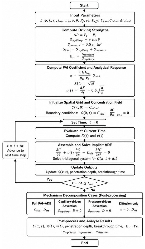
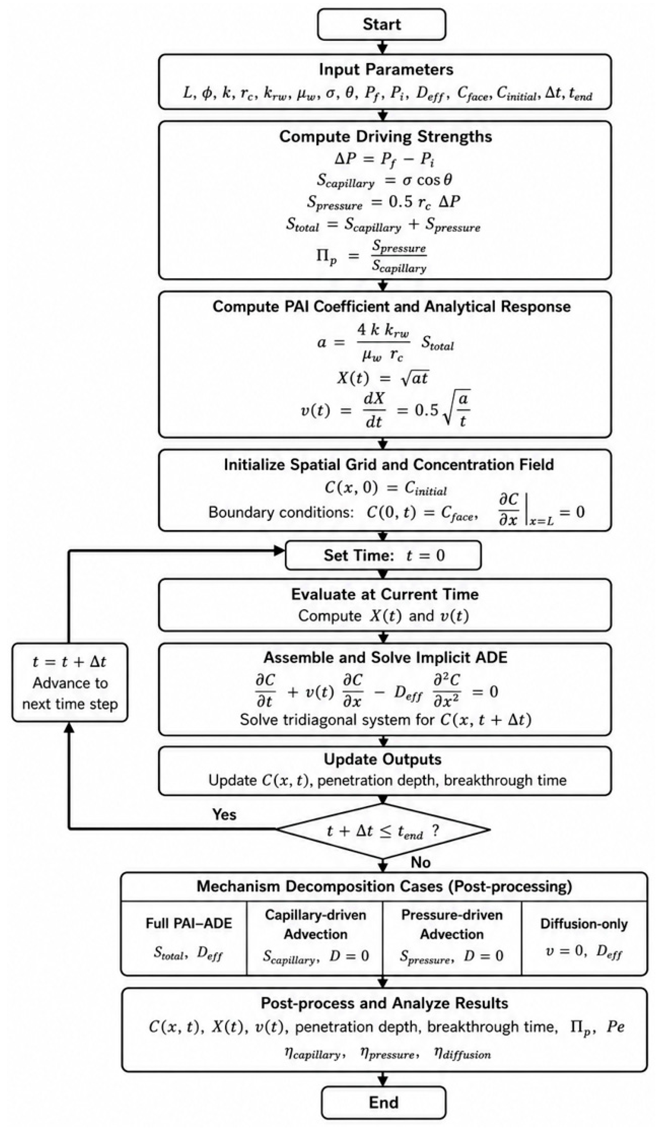
Figure 1 summarizes the computational workflow of the presented PAI-ADE framework. The workflow begins with the definition of the matrix geometry, rock–fluid properties, pressure condition, concentration values, effective diffusion coefficient, time step, and simulation duration. Based on these inputs, the capillary-driving and pressure-driving strengths are calculated and combined to determine the total PAI driving term. The PAI coefficient, pressure–capillary ratio, analytical imbibition-front position, and PAI-derived velocity are then evaluated. The verified PAI-derived velocity is subsequently supplied to the ADE solver described in Section 3.1. The transport calculation is advanced until the final simulation time or the specified breakthrough criterion is reached. The main recorded outputs include the concentration profile, imbibition-front position, PAI-derived velocity, concentration penetration depth, and breakthrough time when applicable. The workflow also includes diagnostic limiting-case simulations used for mechanism comparison. These cases follow the same computational sequence but selectively retain or remove capillary driving, pressure driving, and diffusion according to the case definitions introduced in Section 4.1. After the transport simulations are completed, the front-scale Péclet number and normalized mechanism weights are calculated for dimensionless interpretation. These quantities link the profile-based transport behavior to the relative influence of capillary-driven advection, pressure-driven advection, and diffusion.

Figure 1. Computational workflow of the pressure-assisted imbibition and species-transport framework.

4. Results and Discussion

4.1. Simulation Parameters

Two porous-media models are evaluated using the same PAI-ADE formulation as summarized in Table 1. The Ultra-Low-Permeability Matrix, hereafter referred to as the Ultra-Low Matrix, is the primary target case of this study and represents a nanodarcy-scale tight- or shale-gas matrix with absolute permeability of $1.0\times {10}^{-4}$ mD, equivalent to 100 nD. The High-Perm Matrix is included as a contrasting reference case to illustrate how the same formulation behaves when pressure-driven advection becomes much stronger. The two demonstrative cases are used to illustrate the application of the proposed mechanism-decomposition framework under distinct prescribed porous-medium conditions. They are not treated as points in a permeability or pore-size sensitivity study. Within each case, the complete set of rock–fluid parameters is held fixed, while the diagnostic limiting cases selectively retain or remove pressure-driven advection, capillary-driven advection, and diffusion to evaluate their relative roles.

Table 1. Input parameters for the Ultra-Low Matrix and High-Perm Matrix cases.

Parameter	Symbol	Unit	Ultra-Low Matrix	High-Perm Matrix
Matrix Length	$L$	Cm	500	500
Porosity	$\varphi$	-	0.1	0.1
Effective Diffusion Coefficient	$D_{eff}$	cm2/s	1.0 × 10−5	1.0 × 10−5
Absolute Permeability	$k$	mD	1.0 × 10−4	100
Equivalent Pore Radius	$r_c$	cm	5.0 × 10−7	5.0 × 10−4
Wetting-Fluid Viscosity	${\mu }_w$	cP	1.0	1.0
Wetting-Phase Relative Permeability	$k_{rw}$	-	0.5	0.5
Interfacial Tension	$\sigma$	dyne/cm	40	40
Contact Angle	$\theta$	degree	30	30
Fracture Pressure	$P_F$	atm	520	520
Matrix/Reservoir Pressure	$P_R$	atm	500	500
Initial Concentration	$C_{initial}$	-	0	0
Fracture Face Concentration	$C_{face}$	-	1.0	1.0

1 atm = 1.01325 × 10⁶ dyne/cm². 1 mD = 9.869233 × 10⁻¹² cm². 1 cP = 1.0 × 10⁻² g/(cm-s).

The parameters listed in Table 1 are selected to define two demonstrative cases rather than to calibrate a specific geological formation. The Ultra-Low Matrix represents a nanodarcy-scale tight- or shale-gas matrix condition [5], whereas the High-Perm Matrix is prescribed as a contrasting reference condition. The selected effective diffusion coefficient is representative of aqueous-species diffusion in shale and other low-permeability porous media [16]. The equivalent pore radius, front wetting-phase relative permeability, fluid properties, domain length, pressure conditions, and normalized concentrations are prescribed parameters used to define the two model cases and their initial and boundary conditions.

The reference pressure-assistance condition is defined by $P_F=520$ atm and $P_R=500$ atm, corresponding to $\mathsf{\Delta }P=20$ atm. A weak pressure-assistance condition, $\mathsf{\Delta }P=2$ atm, is additionally used in Section 4.5 to examine how the dimensionless mechanism weights shift when pressure support is reduced. For each porous-media model, four transport cases are evaluated to support the mechanism comparison. The Full PAI-ADE case retains capillary driving, pressure driving, and effective diffusion. The Capillary-driven Advection case retains only capillary driving and removes diffusion. The Pressure-driven Advection case retains only pressure driving and removes diffusion. The Diffusion-only case removes PAI-derived advection and retains only effective diffusion.

4.2. Verification of the Pressure-Assisted Imbibition Model

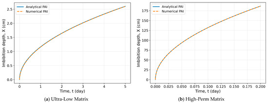
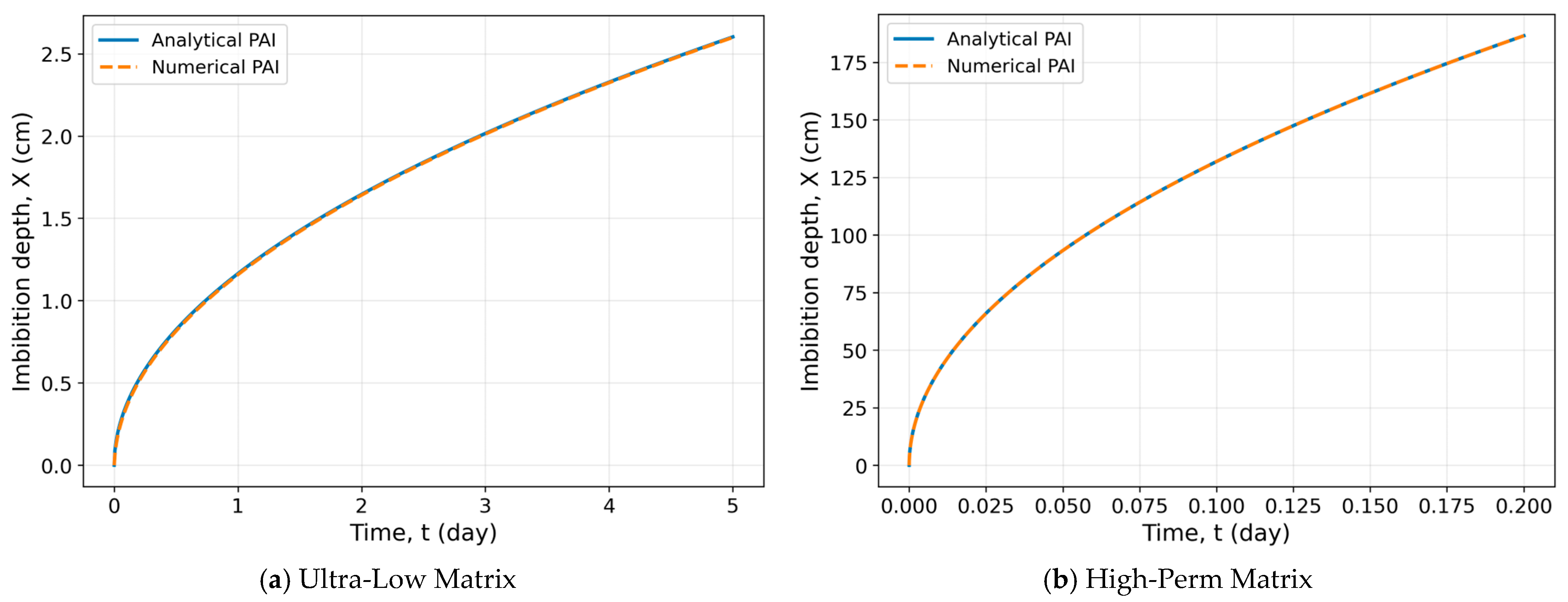
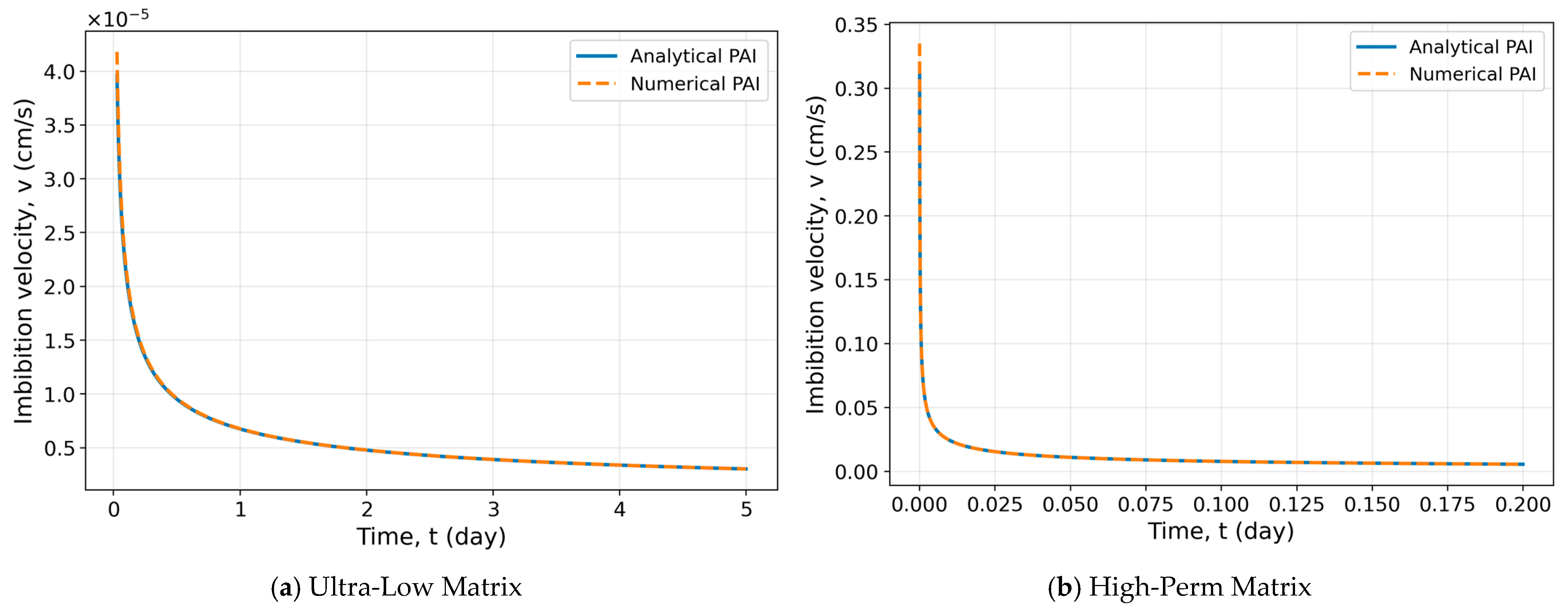
Because the coupled transport simulations use the analytical PAI-derived velocity as the advective input, the analytical solution was compared with an independent numerical solution of the full transient PAI governing equation. The numerical formulation retains the second-order acceleration term, whereas the analytical solution represents the post-start-up, viscous-dominated reduction in which this term is neglected. Consequently, the comparison evaluates both the numerical implementation and the influence of neglecting inertia over the investigated time intervals. Figure 2 and Figure 3 compare the analytical and full transient numerical imbibition-depth and velocity histories for the Ultra-Low Matrix and High-Perm Matrix under the reference pressure-assistance condition.

Figure 2. Comparison of analytical and numerical PAI imbibition-depth histories for (a) Ultra-Low Matrix and (b) High-Perm Matrix under the reference pressure-assistance condition, $∆P=20 \mathrm{a}\mathrm{t}\mathrm{m}$.

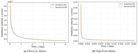
Figure 3. Comparison of analytical and numerical PAI-derived velocity histories for (a) Ultra-Low Matrix and (b) High-Perm Matrix under the reference pressure-assistance condition, $∆P=20 \mathrm{a}\mathrm{t}\mathrm{m}$.

For the Ultra-Low Matrix, Figure 2a and Figure 3a show close agreement between the analytical and numerical PAI solutions over the 5-day verification period. At the final time, the analytical imbibition depth is 2.602 cm, while the numerical imbibition depth is 2.599 cm. The depth comparison gives $R^2=0.9999$. The velocity comparison is more sensitive to the earliest time steps because the analytical velocity is singular at t = 0, but after excluding the undefined initial value, the velocity comparison still gives $R^2=0.9913$. At the final time, the analytical and numerical velocities are 3.012 × 10⁻⁶ cm/s and 3.016 × 10⁻⁶ cm/s, respectively. For the High-Perm Matrix, Figure 2b and Figure 3b show similarly close agreement over a shorter 0.2-day verification period. The shorter interval is used because the larger permeability and pore radius lead to much faster imbibition-front advancement. At the final time, the analytical imbibition depth is 186.54 cm, while the numerical imbibition depth is 186.52 cm. The depth comparison gives $R^2\approx 1.0000$. The velocity comparison, excluding the undefined initial value, gives $R^2=0.9952$. At the final time, the analytical and numerical velocities are 5.3975 × 10⁻³ cm/s and 5.3980 × 10⁻³ cm/s, respectively.

The close agreement between the full transient numerical solution and the reduced analytical solution shows that retaining the acceleration term produces a negligible change in the reported imbibition-depth and velocity histories over the investigated time intervals. This result is consistent with the scale analysis in Appendix A, which demonstrates that the numerical verification times are many orders of magnitude longer than the corresponding inertial relaxation times. The analytical PAI-derived velocity can therefore be used consistently as the advective input for the subsequent transport calculations within the reported parameter and time ranges. The formulation also recovers the classical spontaneous-imbibition limit. As shown in Appendix A, setting $\mathsf{\Delta }P=0$, $k_{rw}=1$, and $k=r_c^2/8$ reduces the PAI solution to the Lucas–Washburn relation. This confirms that the capillary component is consistent with the established pure-capillary behavior, while the general formulation additionally accounts for pressure assistance.

4.3. Coupled PAI-ADE Species Transport

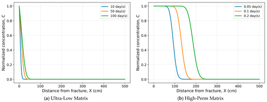
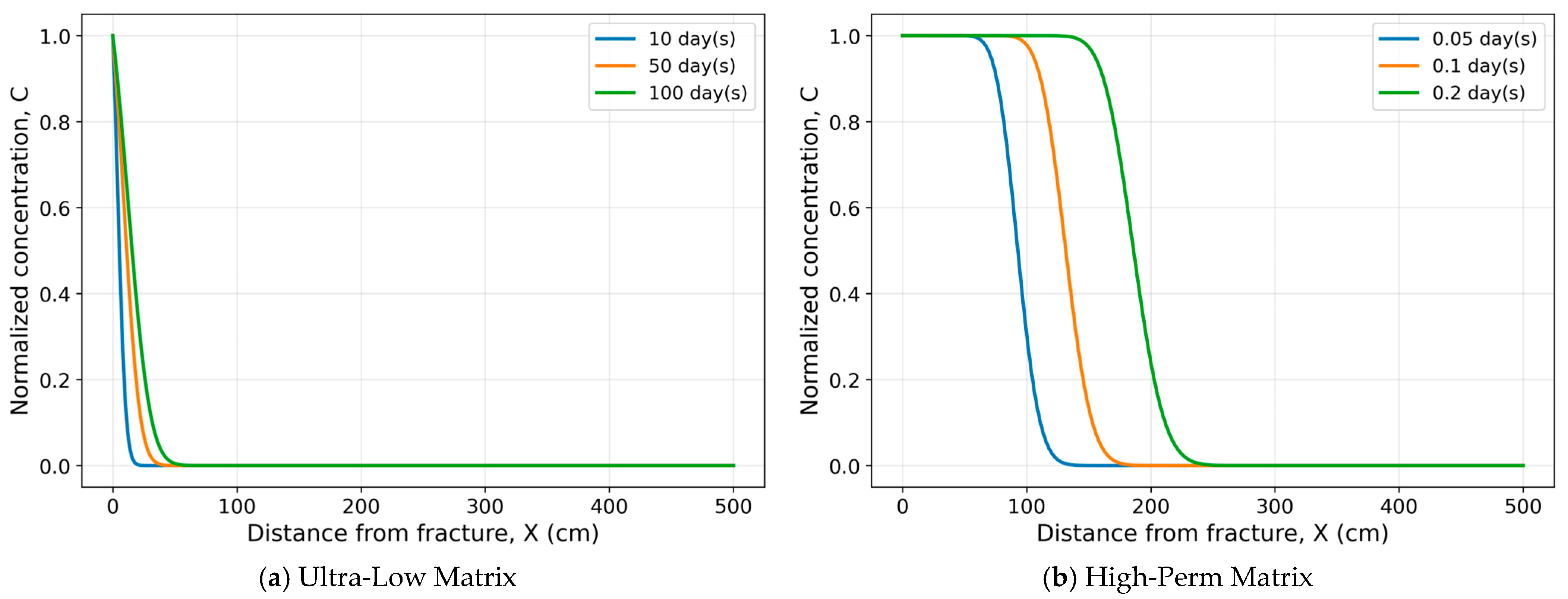
The verified PAI-derived velocity was next coupled with the ADE to evaluate species transport from the fracture face into the matrix. Figure 4 presents the Full PAI-ADE concentration profiles for the two matrix cases under the reference pressure-assistance condition. Different profile times are used because the two media have substantially different imbibition and transport rates: the Ultra-Low Matrix is shown at 10, 50, and 100 days, while the High-Perm Matrix is shown at 0.05, 0.10, and 0.20 day.

Figure 4. Full PAI-ADE concentration profiles for (a) the Ultra-Low Matrix at 10, 50, and 100 days and (b) the High-Perm Matrix at 0.05, 0.10, and 0.20 day under the reference pressure-assistance condition, $∆P=20 \mathrm{a}\mathrm{t}\mathrm{m}$.

For the Ultra-Low Matrix, Figure 4a shows that species transport remains confined to the near-fracture region over the simulated time interval. The PAI front advances from 3.680 cm at 10 days to 8.229 cm at 50 days and 11.638 cm at 100 days. Over the same period, the PAI-derived velocity decreases from 2.130 × 10⁻⁶ cm/s to 9.524 × 10⁻⁷ cm/s and 6.735 × 10⁻⁷ cm/s, respectively. The concentration profiles therefore show a slowly advancing and gradually spreading transport front. For the High-Perm Matrix, Figure 4b shows a much faster concentration-front advancement. The PAI front reaches 93.269 cm at 0.05 day, 131.902 cm at 0.10 day, and 186.538 cm at 0.20 day. Although the PAI-derived velocity decreases with time, it remains much larger than that in the Ultra-Low Matrix, decreasing from 1.080 × 10⁻² cm/s at 0.05 day to 7.633 × 10⁻³ cm/s at 0.10 day and 5.398 × 10⁻³ cm/s at 0.20 day. Thus, the High-Perm Matrix exhibits much faster near-fracture species penetration than the Ultra-Low Matrix, even though the concentration front does not reach the distal boundary within the plotted time window.

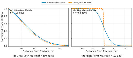
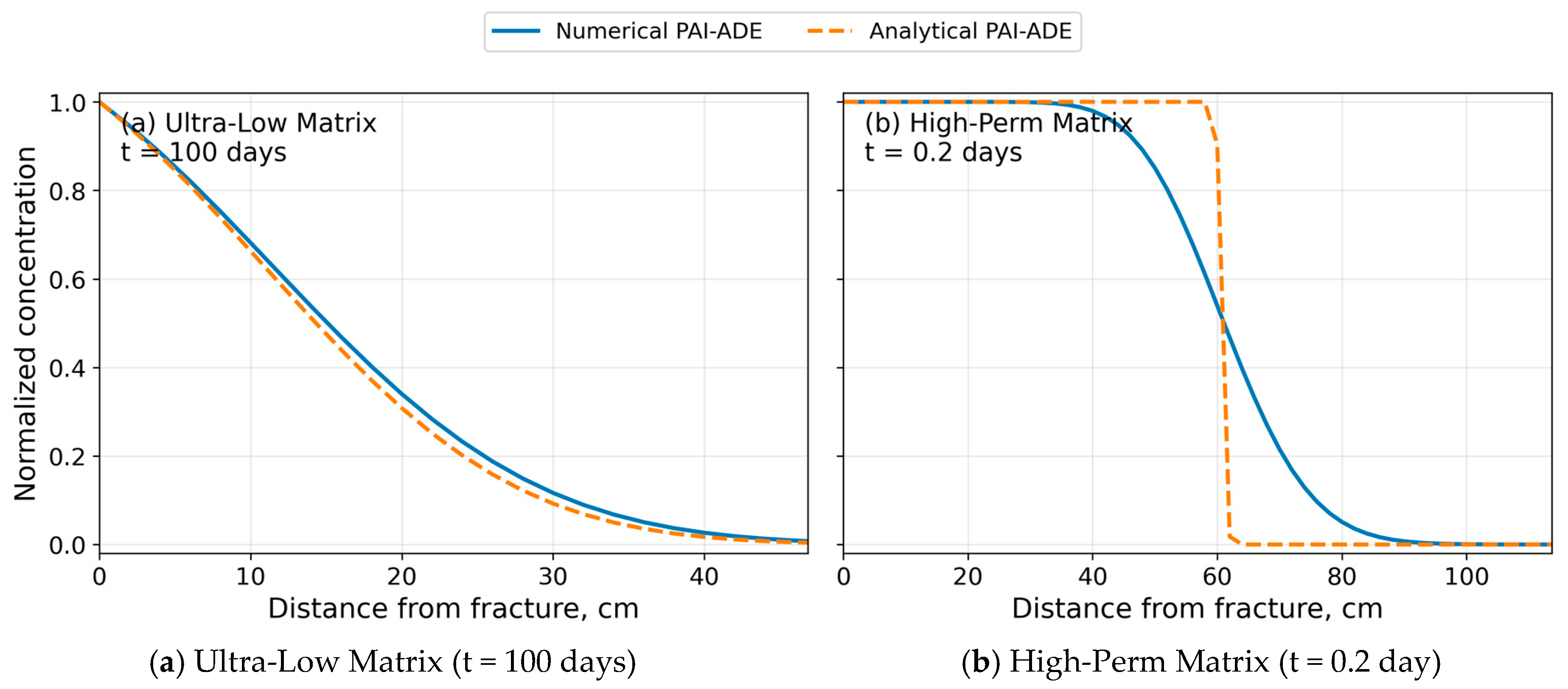
To assess the numerical diffusion associated with the first-order upwind approximation, the numerical PAI-ADE profiles were compared with the corresponding analytical solutions for the same physical cases and reporting times used in the main analysis. Because concentration-front advancement is a primary output of the present mechanism comparison, the numerical error was quantified using the relative difference in the $C=0.1$ front position, $E_f={\displaystyle \frac{\left|x_{0.1}^{num}{-x}_{0.1}^{ana}\right|}{x_{0.1}^{ana}}}$. For the Ultra-Low Matrix at 100 days, the numerical and analytical $C=0.1$ front positions are 31.85 and 30.00 cm, respectively, corresponding to a relative difference of 6.2%. For the High-Perm Matrix at 0.20 day, the corresponding positions are 211.60 and 187.77 cm, giving a relative difference of 12.7%. Figure 5 shows that the larger High-Perm difference is primarily associated with numerical broadening of the sharp low-concentration front. The numerical and analytical $C=0.5$ positions are 186.16 and 186.79 cm, respectively, differing by only 0.33%, which confirms that the bulk advective-front position is preserved. Thus, the first-order scheme has a limited influence on the front advancement of the primary Ultra-Low Matrix case. In the High-Perm reference case, numerical diffusion affects the low-concentration tail and the corresponding $C=0.1$ distance, but it does not alter the bulk front position or the identification of this case as the pressure-advection-dominated limit.

Figure 5. Comparison of the numerical and analytical PAI-ADE concentration profiles obtained using the same PAI-derived transient velocity and physical parameters for (a) the Ultra-Low Matrix at 100 days and (b) the High-Perm Matrix at 0.20 day under the reference pressure-assistance condition, $\mathsf{\Delta }P=20$ atm.

4.4. Mechanism Decomposition of Species Transport

The mechanism-decomposition analysis was performed as a diagnostic limiting-case comparison. The Full PAI-ADE case uses the combined capillary-pressure PAI velocity and effective diffusion. The three limiting cases selectively isolate reduced mechanisms: Capillary-driven Advection retains only the capillary-driven PAI velocity and removes diffusion, Pressure-driven Advection retains only the pressure-driven PAI velocity and removes diffusion, and Diffusion-only removes PAI advection and retains effective diffusion. These limiting cases are independent simulations and are not additive components of the Full PAI-ADE concentration profile.

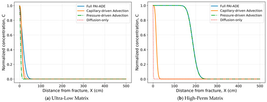
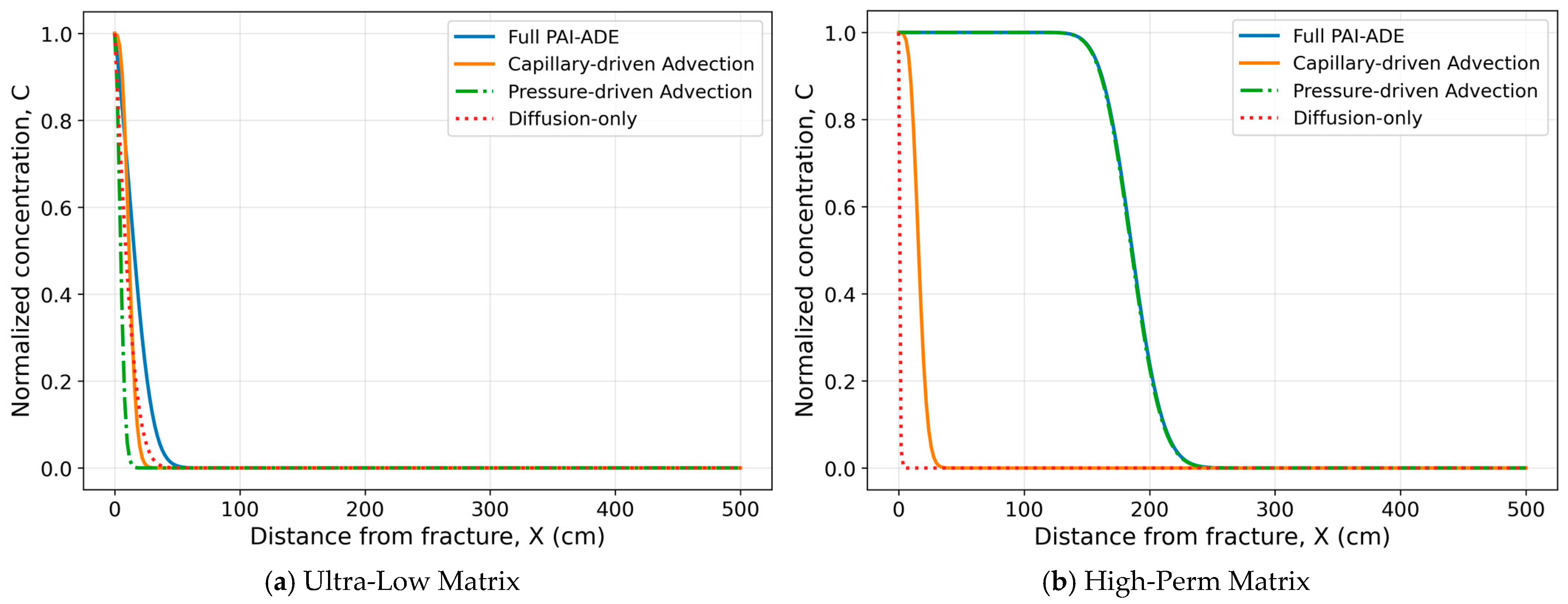
Figure 6 compares the resulting profiles for the Ultra-Low Matrix at 100 days and the High-Perm Matrix at 0.20 day. For the Ultra-Low Matrix, Figure 6a shows that all four cases remain confined to the near-fracture region. Using ($C=0.1$) as the front indicator, the Full PAI-ADE front reaches approximately 31.9 cm. The corresponding front locations are approximately 18.0 cm for Capillary-driven Advection, 9.2 cm for Pressure-driven Advection, and 21.7 cm for Diffusion-only. The Diffusion-only profile spreads farther than the single-advection cases at this threshold because it evolves over the full 100-day period under a fixed fracture-face concentration, but it remains a diffuse near-fracture profile rather than a sharp advective front. For the High-Perm Matrix, Figure 6b shows a different mechanism response. The Full PAI-ADE and Pressure-driven Advection profiles almost overlap, indicating that pressure-driven advection controls the Full PAI-ADE response under the reference pressure-assistance condition. Using the same front indicator ($C=0.1$), the Full PAI-ADE and Pressure-driven Advection fronts reach approximately 211.6 cm and 210.9 cm, respectively. In contrast, the Capillary-driven Advection front reaches approximately 23.6 cm, and the Diffusion-only front reaches approximately 1.9 cm. The contrast between Figure 6a,b shows that the two matrix cases differ not only in transport rate but also in the reduced mechanism that most closely reproduces the full response.

Figure 6. Mechanism-decomposition concentration profiles for (a) the Ultra-Low Matrix at 100 days and (b) the High-Perm Matrix at 0.2 day under the reference pressure-assistance condition, $∆P=20 \mathrm{a}\mathrm{t}\mathrm{m}$. The Full PAI-ADE case is compared with three diagnostic limiting cases: Capillary-driven Advection, Pressure-driven Advection, and Diffusion-only.

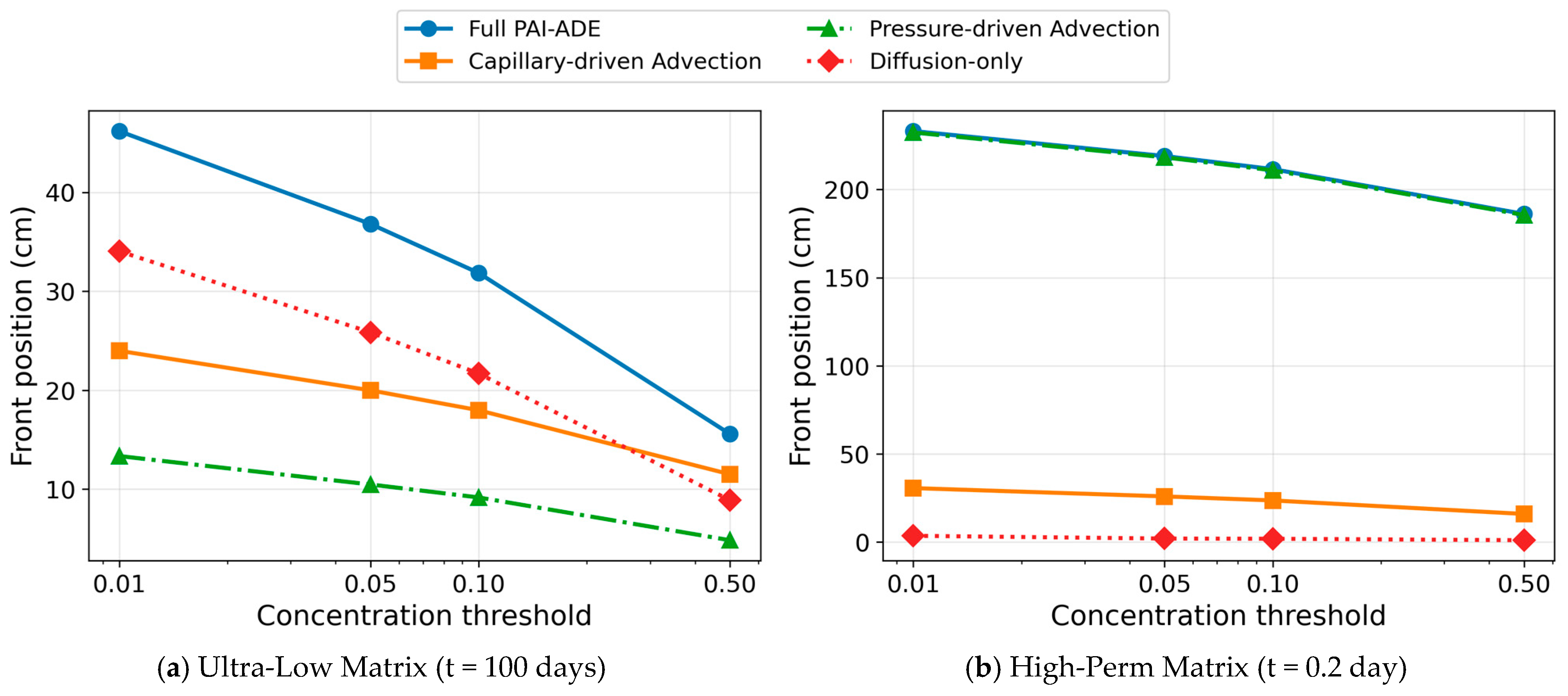
To examine whether the mechanism interpretation depends on the selected concentration-front criterion, the front positions were additionally evaluated using $C=0.01$, 0.05, 0.10, and 0.50. Agreement between each reduced-case profile and the Full PAI-ADE profile was also quantified using the normalized integrated absolute profile error as shown in Equation (11). A smaller $E_{\mathrm{p}\mathrm{r}\mathrm{o}\mathrm{f}\mathrm{i}\mathrm{l}\mathrm{e}}$ indicates closer agreement with the complete Full PAI-ADE concentration profile

$$E_{\mathrm{p}\mathrm{r}\mathrm{o}\mathrm{f}\mathrm{i}\mathrm{l}\mathrm{e}}={\displaystyle \frac{{\int }_0^L\left|C_{reduced}\left(x\right)-C_{full}\left(x\right)\right|dx }{{\int }_0^L{C}_{full}\left(x\right)dx}}$$

(11)

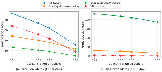
As shown in Figure 7, the front positions of all cases decrease as the concentration threshold increases because a higher concentration level is reached closer to the fracture face, whereas a lower threshold captures the more distant low-concentration portion of the profile. The influence of threshold selection differs between the two matrix cases. For the Ultra-Low Matrix, the Diffusion-only front extends farther than the Capillary-driven Advection front at $C=0.01$, 0.05, and 0.10, whereas the Capillary-driven Advection front extends farther at $C=0.50$. The Pressure-driven Advection front remains the shortest at all four thresholds. This change in ordering indicates that diffusion contributes more strongly to the low-concentration tail, while capillary-driven transport becomes relatively more important in the higher-concentration region. The normalized profile errors are 0.355 for Capillary-driven Advection, 0.379 for Diffusion-only, and 0.696 for Pressure-driven Advection. Therefore, the selected threshold affects the relative apparent importance of diffusion and capillary-driven transport, but neither mechanism alone reproduces the Full PAI-ADE profile. The Ultra-Low Matrix is consequently interpreted as a mixed diffusion–capillary response rather than as being controlled by a single reduced mechanism. For the High-Perm Matrix, the Full PAI-ADE and Pressure-driven Advection fronts remain nearly coincident at all four thresholds, and the ordering remains Pressure-driven Advection, Capillary-driven Advection, and Diffusion-only. The normalized profile error for Pressure-driven Advection is 0.003, compared with 0.913 for Capillary-driven Advection and 0.994 for Diffusion-only. Thus, the pressure-advection-dominated classification is insensitive to the selected concentration threshold.

Figure 7. Sensitivity of the concentration-front position to the selected threshold for (a) the Ultra-Low Matrix at 100 days and (b) the High-Perm Matrix at 0.20 day under the reference pressure-assistance condition, $\mathsf{\Delta }P=20$ atm. Front positions are evaluated using $C=0.01$, 0.05, 0.10, and 0.50.

4.5. Dimensionless Mechanism-Weight Analysis

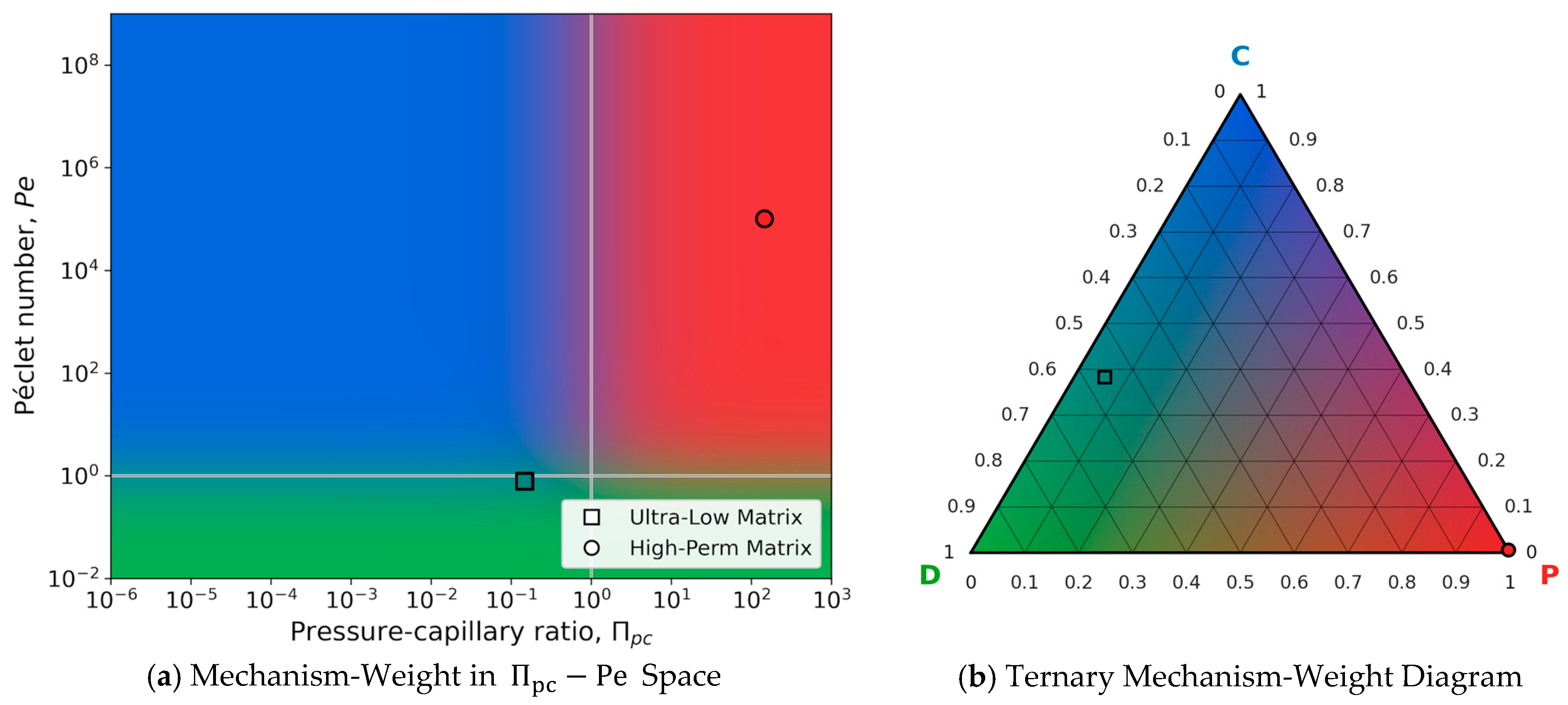
The profiles in Section 4.4 provide a direct mechanism comparison, but they depend on the selected profile time for each matrix case. To provide a more compact interpretation, the two matrix cases are mapped into ${\mathsf{\Pi }}_{\mathrm{p}\mathrm{c}}-\mathrm{P}\mathrm{e}$ space and converted into normalized mechanism weights. In this space, ${\mathsf{\Pi }}_{\mathrm{p}\mathrm{c}}$ measures the relative strength of pressure driving to capillary driving, while $\mathrm{P}\mathrm{e}$ measures the relative importance of advection to diffusion. Because the front-scale $\mathrm{P}\mathrm{e}$ is computed from the analytical PAI formulation, each porous-media model appears as a fixed point for a given pressure-assistance condition. Figure 8 and Figure 9 compare the reference condition, $∆P=20 \mathrm{a}\mathrm{t}\mathrm{m}$, with a weak pressure-assistance condition with $∆P=2 \mathrm{a}\mathrm{t}\mathrm{m}$.

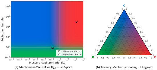
Figure 8. Dimensionless mechanism-weight interpretation for the reference pressure-assistance condition, ΔP = 20 atm. (a) Locations of the Ultra-Low Matrix and High-Perm Matrix in ${\mathsf{\Pi }}_{\mathrm{p}\mathrm{c}}-\mathrm{P}\mathrm{e}$ space. (b) Ternary mechanism-weight diagram showing ${\mathsf{\eta }}_{\mathrm{c}\mathrm{a}\mathrm{p}\mathrm{i}\mathrm{l}\mathrm{l}\mathrm{a}\mathrm{r}\mathrm{y}}$, ${\mathsf{\eta }}_{\mathrm{p}\mathrm{r}\mathrm{e}\mathrm{s}\mathrm{s}\mathrm{u}\mathrm{r}\mathrm{e}}$, and ${\mathsf{\eta }}_{\mathrm{d}\mathrm{i}\mathrm{f}\mathrm{f}\mathrm{u}\mathrm{s}\mathrm{i}\mathrm{o}\mathrm{n}}$ for the two matrix cases. The letters C, P, and D denote capillary-driven advection, pressure-driven advection, and diffusion, respectively.

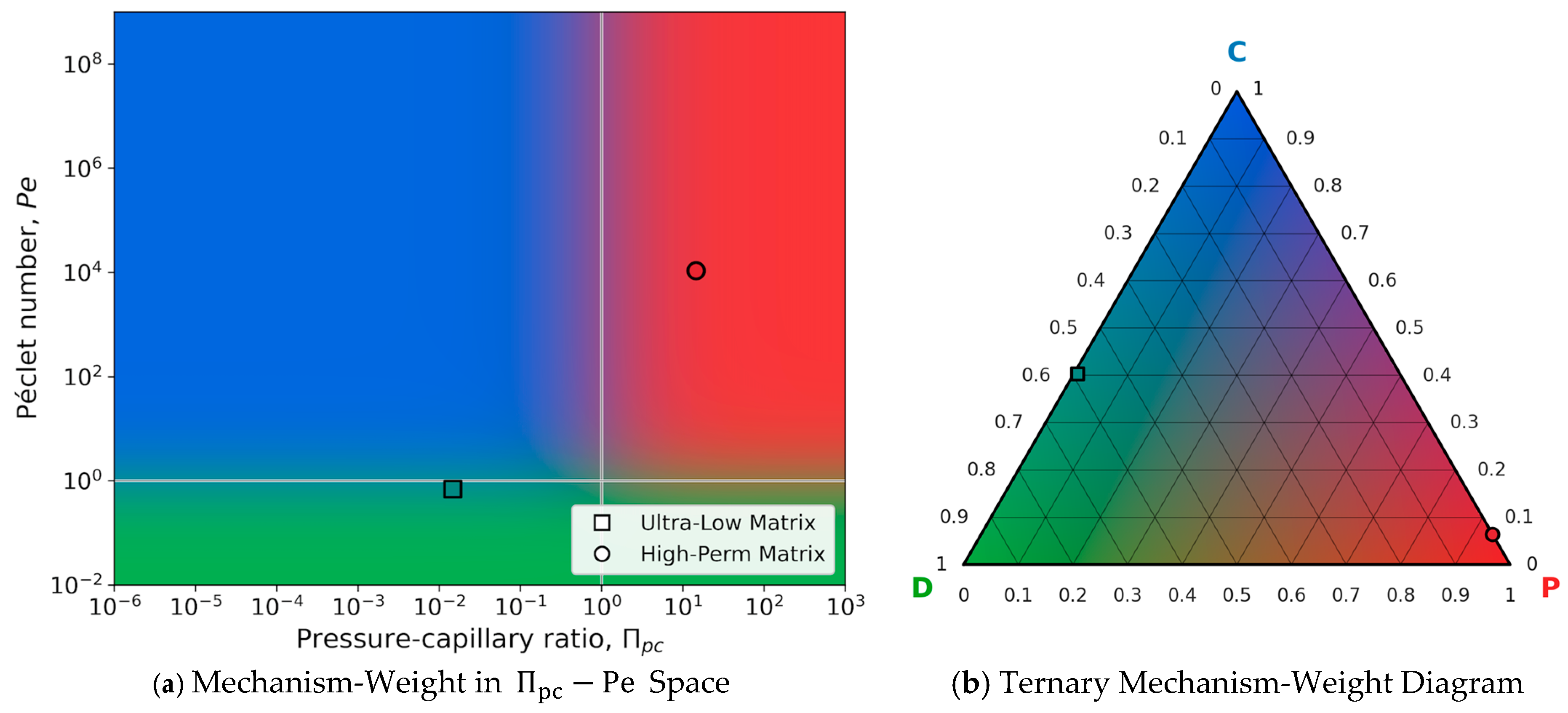
Figure 9. Dimensionless mechanism-weight interpretation for the weak pressure-assistance condition, ΔP = 2 atm. (a) Locations of the Ultra-Low Matrix and High-Perm Matrix in ${\mathsf{\Pi }}_{\mathrm{p}\mathrm{c}}-\mathrm{P}\mathrm{e}$ space. (b) Ternary mechanism-weight diagram showing ${\mathsf{\eta }}_{\mathrm{c}\mathrm{a}\mathrm{p}\mathrm{i}\mathrm{l}\mathrm{l}\mathrm{a}\mathrm{r}\mathrm{y}}$, ${\mathsf{\eta }}_{\mathrm{p}\mathrm{r}\mathrm{e}\mathrm{s}\mathrm{s}\mathrm{u}\mathrm{r}\mathrm{e}}$, and ${\mathsf{\eta }}_{\mathrm{d}\mathrm{i}\mathrm{f}\mathrm{f}\mathrm{u}\mathrm{s}\mathrm{i}\mathrm{o}\mathrm{n}}$ for the two matrix cases. The letters C, P, and D denote capillary-driven advection, pressure-driven advection, and diffusion, respectively.

Figure 8 summarizes the dimensionless interpretation for ΔP = 20 atm. In Figure 8a, the background map provides a qualitative visualization of the dominant mechanism over a broad range of pressure–capillary and advection–diffusion conditions, while the reference lines ${\mathsf{\Pi }}_{\mathrm{p}\mathrm{c}}=1$ and $\mathrm{P}\mathrm{e}=1$ indicate approximate transitions between capillary versus pressure driving and diffusion versus advection tendency. The Ultra-Low Matrix is located at ${\mathsf{\Pi }}_{\mathrm{p}\mathrm{c}}=0.146$ and $\mathrm{P}\mathrm{e}=0.784$. The ternary diagram in Figure 8b gives ${\mathsf{\eta }}_{\mathrm{c}\mathrm{a}\mathrm{p}\mathrm{i}\mathrm{l}\mathrm{l}\mathrm{a}\mathrm{r}\mathrm{y}}=0.383$, ${\mathsf{\eta }}_{\mathrm{p}\mathrm{r}\mathrm{e}\mathrm{s}\mathrm{s}\mathrm{u}\mathrm{r}\mathrm{e}}=0.056$, and ${\mathsf{\eta }}_{\mathrm{d}\mathrm{i}\mathrm{f}\mathrm{f}\mathrm{u}\mathrm{s}\mathrm{i}\mathrm{o}\mathrm{n}}=0.561$ indicating that diffusion has the largest normalized weight, with capillary-driven advection as the secondary contribution. In contrast, the High-Perm Matrix is located at ${\mathsf{\Pi }}_{\mathrm{p}\mathrm{c}}=146.3$ and $\mathrm{P}\mathrm{e}={10}^5$. Its ternary weights are ${\mathsf{\eta }}_{\mathrm{c}\mathrm{a}\mathrm{p}\mathrm{i}\mathrm{l}\mathrm{l}\mathrm{a}\mathrm{r}\mathrm{y}}=0.0068$, ${\mathsf{\eta }}_{\mathrm{p}\mathrm{r}\mathrm{e}\mathrm{s}\mathrm{s}\mathrm{u}\mathrm{r}\mathrm{e}}=0.9932$, and ${\mathsf{\eta }}_{\mathrm{d}\mathrm{i}\mathrm{f}\mathrm{f}\mathrm{u}\mathrm{s}\mathrm{i}\mathrm{o}\mathrm{n}}=0.00001$. This point lies deep in the pressure-driven advection region, consistent with the close overlap between the Full PAI-ADE and Pressure-driven Advection profiles in Figure 6b.

To evaluate whether this interpretation is controlled by the selected pressure-assistance level, Figure 9 repeats the same dimensionless analysis for a weak pressure-assistance condition, ΔP = 2 atm. Reducing ΔP shifts both matrix cases toward smaller ${\mathsf{\Pi }}_{\mathrm{p}\mathrm{c}}$ values and lower advective strength, but the two media respond differently. For the Ultra-Low Matrix, ${\mathsf{\Pi }}_{\mathrm{p}\mathrm{c}}$ decreases to 0.0146 and $\mathrm{P}\mathrm{e}$ decreases to 0.694. The corresponding weights are ${\mathsf{\eta }}_{\mathrm{c}\mathrm{a}\mathrm{p}\mathrm{i}\mathrm{l}\mathrm{l}\mathrm{a}\mathrm{r}\mathrm{y}}=0.404$, ${\mathsf{\eta }}_{\mathrm{p}\mathrm{r}\mathrm{e}\mathrm{s}\mathrm{s}\mathrm{u}\mathrm{r}\mathrm{e}}=0.006$ and ${\mathsf{\eta }}_{\mathrm{d}\mathrm{i}\mathrm{f}\mathrm{f}\mathrm{u}\mathrm{s}\mathrm{i}\mathrm{o}\mathrm{n}}=0.590$. Therefore, the Ultra-Low Matrix remains diffusion-dominant in the normalized mechanism-weight sense, while the pressure-driven contribution becomes nearly negligible. For the High-Perm Matrix, ${\mathsf{\Pi }}_{\mathrm{p}\mathrm{c}}$ decreases from 146.250 to 14.625 and $\mathrm{P}\mathrm{e}$ decreases from ${10}^5$ to ${10}^4$. Despite this reduction, the corresponding weights remain strongly pressure-driven, with ${\mathsf{\eta }}_{\mathrm{c}\mathrm{a}\mathrm{p}\mathrm{i}\mathrm{l}\mathrm{l}\mathrm{a}\mathrm{r}\mathrm{y}}=0.0640$, ${\mathsf{\eta }}_{\mathrm{p}\mathrm{r}\mathrm{e}\mathrm{s}\mathrm{s}\mathrm{u}\mathrm{r}\mathrm{e}}=0.9359$, and ${\mathsf{\eta }}_{\mathrm{d}\mathrm{i}\mathrm{f}\mathrm{f}\mathrm{u}\mathrm{s}\mathrm{i}\mathrm{o}\mathrm{n}}=0.0001$. Although weaker pressure assistance increases the relative capillary weight, the High-Perm Matrix remains pressure-advection dominated. Overall, Figure 8 and Figure 9 show that the Ultra-Low Matrix is governed by diffusion–capillary balance over this pressure range, whereas the High-Perm Matrix remains dominated by pressure-driven advection even under weak pressure assistance.

From an application perspective, separating pressure-driven advection, capillary-driven advection, and diffusion helps distinguish transport controlled primarily by operational pressure conditions from that governed by intrinsic rock–fluid properties. This distinction provides a mechanism-based basis for interpreting fracturing-fluid retention, near-fracture species penetration, and flowback-related behavior, and for identifying whether pressure management or fluid–rock interactions are likely to be more influential under a prescribed reservoir condition.

4.6. Assumptions and Limitations

The present formulation is a simplified front-based model for a homogeneous and isotropic matrix with one-dimensional transport normal to the fracture face. The matrix is assumed to be initially partially water-saturated and to contain connected aqueous pathways for dissolved-species transport. Wetting-phase invasion is represented by a characteristic moving front with a prescribed front saturation, and the corresponding wetting-phase relative permeability is held constant for each matrix case. Accordingly, the model predicts the characteristic wetting-front position and velocity rather than resolving the complete spatial and temporal evolution of the gas–water saturation distribution.

Local saturation evolution, saturation-dependent diffusion, relative permeability and capillary pressure, gas displacement and compressibility, residual gas trapping, and co-current or counter-current two-phase flow are not explicitly represented. Fracture pressure and species concentration are prescribed at the fracture–matrix boundary, while in-fracture concentration variation, filter-cake effects, chemical reactions, and interfacial mass-transfer resistance are also neglected. These assumptions are consistent with the focus of this study on pressure–capillary–diffusion mechanism analysis. Where fracture-side concentration variation or interfacial resistance is important, the framework may be extended by introducing an interfacial mass-transfer coefficient or a more detailed fracture–matrix coupling condition.

The analytical and numerical comparisons presented in this study constitute theoretical and numerical verification of the model formulation and computational implementation rather than experimental or field-scale validation. The framework has not been calibrated or validated against a matched laboratory experiment or field dataset. Consequently, water blocking, fluid retention, and flowback are treated as application contexts rather than direct predictive outputs. The results should therefore be interpreted as a conceptual and mechanism-based assessment of pressure-assisted imbibition and species transport, rather than as field-calibrated quantitative predictions.

Future extensions should consider saturation-resolved two-phase transport, saturation-dependent transport properties, fracture-side concentration variation, filter-cake and interfacial mass-transfer effects, reactive species transport, and validation against matched laboratory or field datasets.

5. Conclusions

This paper introduced a regime-adaptive pressure-assisted imbibition and advection–diffusion framework for interpreting fracturing-fluid species transport from a hydraulic fracture into a gas-bearing matrix. The PAI model provides a transient imbibition-front position and velocity, which are coupled with the ADE solver. Diagnostic limiting cases and dimensionless mechanism weights are then used to distinguish capillary-driven advection, pressure-driven advection, and diffusion-controlled transport tendencies. Based on the results presented in this study, the following conclusions can be drawn:

• The analytical PAI solution was accurately verified by the independent numerical PAI implementation. For the Ultra-Low Matrix, the analytical and numerical imbibition depths at 5 days were 2.602 cm and 2.599 cm, respectively, with corresponding velocities of 3.012 × 10⁻⁶ cm/s and 3.016 × 10⁻⁶ cm/s. For the High-Perm Matrix, the analytical and numerical imbibition depths at 0.20 day were 186.54 cm and 186.52 cm, respectively, with corresponding velocities of 5.3975 × 10⁻³ cm/s and 5.3980 × 10⁻³ cm/s. Together with the inertial-scale analysis, this agreement shows that neglecting the acceleration term has a negligible effect over the investigated time ranges and supports the use of the analytical PAI-derived velocity in the coupled transport calculations. The formulation also recovers the classical Lucas–Washburn relation under the pure-capillary limit.
• In the primary Ultra-Low Matrix case, the coupled Full PAI-ADE response remains confined to the near-fracture region over the 100-day simulation window. The PAI front advances from 3.680 cm at 10 days to 8.229 cm at 50 days and 11.638 cm at 100 days, while the PAI-derived velocity decreases from 2.130 × 10⁻⁶ cm/s to 9.524 × 10⁻⁷ cm/s and 6.735 × 10⁻⁷ cm/s over the same times. Using $C = 0.1$ as the concentration-front criterion, the Full PAI-ADE species penetration reaches approximately 31.9 cm at 100 days, indicating that dissolved species spread beyond the characteristic PAI front through the connected aqueous pathways represented by the effective diffusion coefficient.
• At 100 days, using $C=0.10$as the concentration-front criterion, the Full PAI-ADE front reaches approximately 31.9 cm, compared with 18.0 cm for Capillary-driven Advection, 9.2 cm for Pressure-driven Advection, and 21.7 cm for Diffusion-only. The multi-threshold analysis shows that diffusion extends farther than capillary-driven advection at $C=0.01$, 0.05, and 0.10, whereas capillary-driven advection extends farther at $C=0.50$. Pressure-driven advection remains the weakest reduced mechanism at all evaluated thresholds. Because neither capillary-driven advection nor diffusion alone reproduces the Full PAI-ADE response, the Ultra-Low Matrix is characterized as a mixed diffusion–capillary regime under the reference pressure condition.
• The High-Perm Matrix serves as a contrasting reference case and approaches the pressure-advection-dominated limit of the formulation. The close alignment between the Full PAI-ADE and Pressure-driven Advection profiles, together with the dimensionless mechanism weights, shows that pressure-driven advection controls the transport response under the reference condition. The analytical benchmark indicates that first-order upwinding broadens the sharp concentration front but does not change this mechanism classification.
• The dimensionless mechanism-weight analysis provides a compact quantitative interpretation of the profile-based results. Under the reference pressure-assistance condition, the Ultra-Low Matrix lies in a diffusion–capillary mixed regime, whereas the High-Perm Matrix lies in a pressure-advection-dominated regime. Reducing the pressure difference from 20 atm to 2 atm shifts both cases toward weaker pressure support, but the Ultra-Low Matrix remains diffusion-dominant with only a small pressure-driven contribution, while the High-Perm Matrix remains pressure-advection dominated. Therefore, the pressure–capillary ratio and front-scale Péclet number provide useful diagnostic indicators for classifying the expected transport regime.

References

- Birdsell, D.T.; Rajaram, H.; Dempsey, D.; Viswanathan, H.S. Hydraulic fracturing fluid migration in the subsurface: A review and expanded modeling results. Water Resour. Res. 2015, 51, 7159–7188. [Google Scholar] [CrossRef] [Scilit]
- Birdsell, D.T.; Rajaram, H.; Lackey, G. Imbibition of hydraulic fracturing fluids into partially saturated shale. Water Resour. Res. 2015, 51, 6787–6796. [Google Scholar] [CrossRef] [Scilit]
- Ge, H.; Yang, L.; Shen, Y.; Ren, K.; Meng, F.; Ji, W.; Wu, S. Experimental investigation of shale imbibition capacity and the factors influencing loss of hydraulic fracturing fluids. Pet. Sci. 2015, 12, 636–650. [Google Scholar] [CrossRef] [Scilit]
- Yang, F.; Zheng, H.; Guo, Q.; Lyu, B.; Nie, S.; Wang, H. Modeling water imbibition and penetration in shales: New insights into the retention of fracturing fluids. Energy Fuels 2021, 35, 13776–13787. [Google Scholar] [CrossRef] [Scilit]
- Li, C.; Singh, H.; Cai, J. Spontaneous imbibition in shale: A review of recent advances. Capillarity 2019, 2, 17–32. [Google Scholar] [CrossRef] [Scilit]
- Yang, L.; Wang, S.; Cai, J.; Gan, Y.; Salama, A. Main controlling factors of fracturing fluid imbibition in shale fracture network. Capillarity 2018, 1, 1–10. [Google Scholar] [CrossRef] [Scilit]
- Gao, Z.; Fan, Y.; Hu, Q.; Jiang, Z.; Cheng, Y.; Xuan, Q. A review of shale wettability characterization using spontaneous imbibition experiments. Mar. Pet. Geol. 2019, 109, 330–338. [Google Scholar] [CrossRef] [Scilit]
- Dehghanpour, H.; Lan, Q.; Saeed, Y.; Fei, H.; Qi, Z. Spontaneous imbibition of brine and oil in gas shales: Effect of water adsorption and resulting microfractures. Energy Fuels 2013, 27, 3039–3049. [Google Scholar] [CrossRef] [Scilit]
- Li, Q.; Jew, A.D.; Brown, G.E., Jr.; Bargar, J.R.; Maher, K. Reactive transport modeling of shale-fluid interactions after imbibition of fracturing fluids. Energy Fuels 2020, 34, 5511–5523. [Google Scholar] [CrossRef] [Scilit]
- Jew, A.D.; Druhan, J.L.; Ihme, M.; Kovscek, A.R.; Battiato, I.; Kaszuba, J.P.; Bargar, J.R.; Brown, G.E. Chemical and reactive transport processes associated with hydraulic fracturing of unconventional oil/gas shales. Chem. Rev. 2022, 122, 9198–9263. [Google Scholar] [CrossRef] [Scilit] [PubMed]
- Lucas, R. Ueber das Zeitgesetz des kapillaren Aufstiegs von Flüssigkeiten. Kolloid-Z. 1918, 23, 15–22. [Google Scholar] [CrossRef] [Scilit]
- Washburn, E.W. The dynamics of capillary flow. Phys. Rev. 1921, 17, 273–283. [Google Scholar] [CrossRef] [Scilit]
- Handy, L.L. Determination of effective capillary pressures for porous media from imbibition data. Trans. AIME 1960, 219, 75–80. [Google Scholar] [CrossRef] [Scilit]
- Cai, J.; Yu, B. A discussion of the effect of tortuosity on the capillary imbibition in porous media. Transp. Porous Media 2011, 89, 251–263. [Google Scholar] [CrossRef] [Scilit]
- Cai, J.; Jin, T.; Kou, J.; Zou, S.; Xiao, J.; Meng, Q. Lucas-Washburn equation-based modeling of capillary-driven flow in porous systems. Langmuir 2021, 37, 1623–1636. [Google Scholar] [CrossRef] [Scilit] [PubMed]
- Ghanbari, E.; Dehghanpour, H. Impact of rock fabric on water imbibition and salt diffusion in gas shales. Int. J. Coal Geol. 2015, 138, 55–67. [Google Scholar] [CrossRef] [Scilit]
- Zhou, Z.; Abass, H.; Li, X.; Bearinger, D.; Frank, W. Mechanisms of imbibition during hydraulic fracturing in shale formations. J. Pet. Sci. Eng. 2016, 141, 125–132. [Google Scholar] [CrossRef] [Scilit]
- Yang, Y.; Wang, S.; Feng, Q.; Cao, X.; Qin, Y.; Shu, C.; Zhong, A.; Wang, X. Imbibition mechanisms of fracturing fluid in shale oil formation: A review from the multiscale perspective. Energy Fuels 2023, 37, 9822–9840. [Google Scholar] [CrossRef] [Scilit]
- Xue, Y.; Li, X.; Wang, L.; Liu, Y.; Cao, X.; Zhang, Y. Mesoscopic damage enhancement in granite under cyclic liquid nitrogen shocks characterized by computed tomography and texture analysis. Int. J. Rock Mech. Min. Sci. 2025, 194, 106217. [Google Scholar] [CrossRef] [Scilit]
- Xue, Y.; Wang, L.; Cao, Z.; Xie, H.; Ranjith, P.G.; Cai, C. Thermo-mechanical degradation and crack evolution of granite subjected to liquid nitrogen cooling cycles for thermal reservoir stimulation. J. Rock Mech. Geotech. Eng. 2026, 18, 3447–3470. [Google Scholar] [CrossRef] [Scilit]
- Di, C.; Tian, F.; Zhao, L.; Deng, P.; Ma, H.; Liu, B.; Peng, L.; Chen, Z. Cooling Effects on Capillary Sealing in CO2-Plume Geothermal Systems: Capillary Pressure Modeling and Leakage Assessment. Environ. Sci. Technol. 2026, 60, 6149–6161. [Google Scholar] [CrossRef] [Scilit] [PubMed]
- Deng, L.; King, M.J. Theoretical investigation of the transition from spontaneous to forced imbibition. SPE J. 2019, 24, 215–229. [Google Scholar] [CrossRef] [Scilit]
- Kurotori, T.; Murugesu, M.P.; Zahasky, C.; Vega, B.; Druhan, J.L.; Benson, S.M.; Kovscek, A.R. Mixed imbibition controls the advance of wetting fluid in multiscale geological media. Adv. Water Resour. 2023, 175, 104429. [Google Scholar] [CrossRef] [Scilit]
- Lu, N.B.; Pahlavan, A.A.; Browne, C.A.; Amchin, D.B.; Stone, H.A.; Datta, S.S. Forced imbibition in stratified porous media. Phys. Rev. Appl. 2020, 14, 054009. [Google Scholar] [CrossRef] [Scilit]
- Gu, Q.; Liu, H.; Wu, L. Preferential imbibition in a dual-permeability pore network. J. Fluid Mech. 2021, 915, A138. [Google Scholar] [CrossRef] [Scilit]
- Mahmood, M.N.; Nguyen, V.; Guo, B. Challenges in mathematical modeling of dynamic mass transfer controlled by capillary and viscous forces in spontaneous fluid imbibition processes. Capillarity 2024, 11, 53–62. [Google Scholar] [CrossRef] [Scilit]
- Bear, J. Dynamics of Fluids in Porous Media; American Elsevier: New York, NY, USA, 1972. [Google Scholar]
- Domenico, P.A.; Schwartz, F.W. Physical and Chemical Hydrogeology, 2nd ed.; Wiley: New York, NY, USA, 1998. [Google Scholar]
- Huysmans, M.; Dassargues, A. Review of the use of Péclet numbers to determine the relative importance of advection and diffusion in low permeability environments. Hydrogeol. J. 2005, 13, 895–904. [Google Scholar] [CrossRef] [Scilit]
- Nordbotten, J.M.; Fernø, M.A.; Flemisch, B.; Kovscek, A.R.; Lie, K.-A.; Both, J.W.; Møyner, O.; Sandve, T.H.; Ahusborde, E.; Bauer, S.; et al. Benchmarking CO2 Storage Simulations: Results from the 11th Society of Petroleum Engineers Comparative Solution Project. Int. J. Greenh. Gas Control 2025, 148, 104519. [Google Scholar] [CrossRef] [Scilit]
- Patankar, S.V. Numerical Heat Transfer and Fluid Flow; Hemisphere Publishing Corporation: Washington, DC, USA, 1980. [Google Scholar]
- Kumar, A.; Jaiswal, D.K.; Kumar, N. Analytical solutions to one-dimensional advection–diffusion equation with variable coefficients in semi-infinite media. J. Hydrol. 2010, 380, 330–337. [Google Scholar] [CrossRef] [Scilit]
Disclaimer/Publisher’s Note: The statements, opinions and data contained in all publications are solely those of the individual author(s) and contributor(s) and not of MDPI and/or the editor(s). MDPI and/or the editor(s) disclaim responsibility for any injury to people or property resulting from any ideas, methods, instructions or products referred to in the content. |
© 2026 by the authors. Licensee MDPI, Basel, Switzerland. This article is an open access article distributed under the terms and conditions of the Creative Commons Attribution (CC BY) license.