


Abstract
The large-scale integration of renewable energy has significantly improved the low-carbon performance of power systems, but has also increased operational uncertainty. Under extreme weather conditions, wind and solar power may experience consecutive days of simultaneous output shortfalls—referred to as “renewable energy drought”—leading to persistently high net load and severe challenges to supply guarantee. To address this issue, this paper proposes a multi-source coordinated supply-guarantee dispatch strategy for consecutive-day renewable energy drought scenarios. First, net load is defined as the total system load minus the available wind and solar output. Based on magnitude and duration thresholds, renewable energy drought events are extracted from historical data to generate representative scarcity scenarios. Second, a multi-source coordinated optimization dispatch model is constructed, incorporating wind power, solar power, thermal units, battery energy storage, and pumped-storage hydro. The objective is to minimize the total system operating cost, which includes thermal fuel cost, start-up/shut-down costs, storage cycling cost, wind/solar curtailment penalty cost, and load shedding penalty cost. The load shedding penalty coefficient is set to a magnitude much higher than conventional costs to highlight the priority of supply guarantee. The model accounts for operational constraints such as minimum up/down times, deep regulation capability, ramping limits of thermal units, and charge/discharge power limits of storage. Taking a provincial power system in China for the year 2030 as a case study, a dispatch case covering four consecutive days (96 time periods) is designed. Based on a baseline scenario, eight groups of sensitivity analyses are conducted to comprehensively investigate the impacts of key factors on the supply-guarantee strategy, including: the minimum up/down time of thermal units, deep regulation capability, load shedding penalty cost, load level, rated energy capacity and charge/discharge efficiency of battery energy storage, rated energy capacity and pumping/generating efficiency of pumped-storage hydro, thermal fuel cost coefficient, and renewable energy capacity. Simulation results show that the proposed strategy can effectively coordinate multiple resources under consecutive-day drought conditions; reducing the minimum up/down time of thermal units improves supply flexibility but increases start-up/shut-down costs; enhancing deep regulation capability optimizes storage utilization and reduces total system cost; the load shedding penalty cost directly determines the trade-off between supply guarantee and economic efficiency; and as load level decreases by 5%, 10%, and 15%, the total system operating cost reduces by approximately 6.3%, 12.5%, and 18.8%, respectively. This study provides a quantitative method and technical support for supply-guarantee dispatch decisions and resource allocation in high-renewable power systems under persistent drought conditions.
1. Introduction
Globally, new energy sources such as wind power and photovoltaics are developing rapidly [1,2,3], and renewable energy power systems are undergoing a low-carbon transition as well as a reconstruction of their operation and dispatch modes [4,5]. In China, the government has set a target to achieve a total installed capacity of wind and solar power of 3.6 billion kilowatts by 2035. In the context of research on renewable energy power systems, renewable energy drought is defined as a novel type of compound event, specifically referring to the phenomenon of persistently and abnormally low wind and solar power generation within a specific region and over a certain timescale (typically lasting from several hours to several weeks) [6]. This term borrows the concept of “drought” from meteorology to characterize the prolonged absence of wind and solar resources within the power system. From the perspective of spatiotemporal distribution characteristics, renewable energy droughts exhibit significant persistence and regionality [7]. Distinct from instantaneous fluctuations, they emphasize the long-term cumulative effect of resource gaps and are typically triggered by stable, large-scale weather systems (such as stationary anticyclones). Such weather systems often lead to a situation over a wide area where “calm winds” coexist with “clear skies”: although there is some photovoltaic (PV) output during the day, PV output drops to zero at night while wind power remains persistently weak, thereby forming a “generation valley” period characterized by a sharp rise in the system’s net load curve.
For the safe and stable operation of a power system, renewable energy droughts pose a serious challenge [8]. During this period, the instantaneous penetration rate of renewable energy drops significantly, and the grid must rely on energy storage system discharge [9,10,11], fast-starting reserve thermal power [12], or large-scale demand response to maintain power balance [13,14,15]. If the system’s flexible resource allocation is insufficient, it will directly lead to power supply tension, potentially triggering controlled load shedding or blackouts. Therefore, in the clean energy transition, the secure dispatch of multiple power sources—including wind, solar, thermal, and storage—under renewable energy droughts has become a core issue in ensuring power supply security.
Extensive research has been carried out on the dispatch problem under renewable energy uncertainty and extreme scenarios. In terms of unit commitment, traditional models describe the regulation capability of thermal units through constraints such as minimum up/down times and ramping limits [16,17,18,19,20,21], and introduce flexible resources such as energy storage [22,23,24] and pumped-storage hydro [25] to smooth net load fluctuations [26]. In extreme scenario modeling [27], some studies adopt robust optimization or stochastic programming methods [28,29], considering the worst-case distribution or typical low-output scenarios of wind and solar power [30]. However, existing research mostly focuses on short-term (e.g., 24 h) periods or single low-output events of renewable energy, and insufficiently explores multi-source coordinated supply-guarantee dispatch strategies under consecutive days (e.g., 96 h) of wind and solar resource drought. Moreover, although most models include a load shedding penalty term to represent supply reliability, they often neglect the impact of detailed economic indicators such as start-up/shut-down costs and storage cycling degradation costs on supply-guarantee dispatch decisions, making it difficult to achieve a quantitative trade-off between supply priority and economic efficiency [31].
Unlike previous studies that primarily focus on short-term (e.g., 24 h) single-event renewable energy shortfalls, this work specifically targets consecutive-day drought scenarios which impose fundamentally different stress characteristics on power systems, including persistently high net load over multiple days, prolonged storage depletion, and cumulative thermal unit cycling stress. In contrast to robust optimization approaches that seek the worst-case distribution over an uncertainty set [28,29] or stochastic programming methods that rely on probabilistic scenarios, our study adopts a deterministic optimization framework based on historically derived scarcity scenarios. This choice is motivated by the practical need for a computationally tractable and interpretable tool that directly supports day-ahead dispatch decisions under predictable extreme drought patterns, without the over-conservatism often associated with robust methods or the computational burden of large-scale scenario-based stochastic programs. Furthermore, while existing renewable energy drought analyses [6,7] primarily focus on event identification and statistical characterization, and prior work on drought-aware dispatch [30] has touched upon multi-source coordination but has not specifically addressed the consecutive-day supply-guarantee challenge, our work bridges this gap by coupling drought event extraction with a detailed multi-source optimization model, thereby translating statistical drought characteristics into actionable supply-guarantee dispatch strategies.
The core novelty of this paper lies in three interconnected aspects. First, we propose a systematic modeling framework that finely characterizes the multi-source coupling operation mechanism driven by supply-guarantee priority under consecutive-day drought conditions, where the load shedding penalty coefficient is set at a significantly higher magnitude than conventional cost terms to explicitly prioritize supply reliability, while storage cycling costs and thermal unit start-up/shut-down costs are simultaneously incorporated to enable a quantitative trade-off between economic efficiency and reliability. Second, unlike most existing models that treat load shedding as a mere slack variable without rigorous economic weighting, our formulation introduces a differentiated penalty structure that allows flexible adjustment according to the actual Value of Lost Load (VOLL) in real-world applications, providing a practical basis for reliability-oriented dispatch. Through systematic comparisons between high and low penalty scenarios, we quantitatively reveal the trade-off between supply security and operational economy. Third, through extensive sensitivity analyses—covering minimum up/down times, deep regulation capability, penalty intensity, load levels, as well as storage and renewable capacity parameters—we systematically reveal the response mechanisms of key operational parameters under extreme scarcity, offering quantitative guidelines for resource configuration and operational decision-making in high-renewable power systems. These contributions collectively advance the understanding and practice of supply-guarantee dispatch under persistent renewable energy droughts, moving beyond conventional unit commitment applications to a dedicated reliability-constrained operational strategy.
To address the above shortcomings, this paper constructs a multi-source coordinated optimization dispatch model incorporating wind power, solar power, thermal units, battery energy storage, and pumped-storage hydro. The objective is to minimize the total system operating cost, which covers thermal fuel cost, start-up/shut-down costs, storage cycling costs (for both BESS and PSH), wind/solar curtailment penalty cost, and load shedding penalty cost. The load shedding penalty coefficient is set to a magnitude much higher than conventional costs to prioritize supply guarantee, while the inclusion of storage cycling costs provides a quantitative basis for balancing supply-guarantee capability against storage lifetime degradation. Based on magnitude and duration thresholds, renewable energy drought events are extracted from historical data to generate representative scarcity scenarios as model inputs.
To systematically verify the proposed model, a 96-period (4 consecutive days) dispatch case is designed for a 2030 provincial power system in China. A baseline scenario with typical parameter configurations is established to comprehensively analyze multi-source coordinated start-up/shut-down, output matching, and capacity support characteristics. On this basis, to comprehensively investigate the impacts of key factors on the supply-guarantee strategy, multiple groups of sensitivity analyses are conducted, covering key parameters such as the minimum up/down time and deep regulation capability of thermal units, load shedding penalty cost, load level, rated energy capacity and charge/discharge/pumping/generating efficiency of BESS and PSH, thermal fuel cost coefficient, and renewable energy capacity.
The remainder of this paper is organized as follows. Section 2 presents the renewable energy drought event extraction rule and the complete mathematical formulation of the multi-source coordinated dispatch model; Section 3 describes the test system parameters and case design, and analyzes the results of the baseline scenario; Section 4 presents the discussion, which analyzes the results of each sensitivity scenario in detail and reveals the impact mechanisms of key parameters; and Section 5 concludes the paper and points out future research directions.
2. Multi-Source Coordinated Supply-Guarantee Dispatch Strategy
2.1. Extraction Rules for Renewable Energy Drought Events
To quantify the severity of insufficient renewable energy output, this paper introduces the core concept of net load. Net load is defined as the total system load minus the available wind and solar power output. It represents the residual power demand that must be met by conventional generators (e.g., thermal units) and flexible resources (e.g., energy storage). The mathematical expression of net load is:
By definition, a higher net load indicates a larger shortfall in renewable energy output relative to demand—i.e., a more severe renewable energy drought. However, judging a meaningful drought event based solely on the net load at a single period is insufficient; the persistence of the high-net-load condition must also be considered. Therefore, this paper identifies renewable energy drought periods from two complementary dimensions: the magnitude threshold and duration threshold.
2.1.1. Magnitude Threshold
A net load magnitude threshold is set. This threshold can be chosen based on the statistical distribution of historical net load series (e.g., the 90th percentile) or as a certain percentage of the total installed capacity of the system (e.g., 80%). When the net load in a period satisfies the following inequality, that period is marked as a drought candidate period:
The magnitude threshold ensures that only periods with significantly high net load (i.e., severe renewable energy shortage) enter the candidate set, thereby excluding minor shortfalls within normal fluctuation ranges.
2.1.2. Duration Threshold
A minimum consecutive duration (e.g., 12 h or 24 h) is set. A continuous block of periods is formally identified as a renewable energy drought event only when the net load consecutively satisfies the magnitude threshold for a length not less than . This criterion ensures that the model captures only persistent, systemic generation shortfalls, rather than short term random fluctuations or isolated anomalies. In practice, can be flexibly set according to the system’s regulation capability, storage capacity, or scheduling horizon: systems with weaker regulation ability should use a larger to reflect more severe drought scenarios.
Based on the above two criteria, renewable energy drought events can be systematically extracted from historical data (or from generated time series). The net load profiles of these events are then used as representative input scenarios for the subsequent multi-source coordinated dispatch model. This approach captures the most adverse operating conditions while avoiding the inclusion of numerous insignificant short-duration low-output periods, thus balancing computational burden and scenario representativeness.
2.2. Key Operation Constraints of Thermal Power Units
Due to the physical characteristics and mechanical limitations of thermal power generation equipment, thermal power units are subject to multiple key operational constraints, including minimum up/down time constraints, state transition logic constraints, start/shut-down mutual exclusivity constraints, ramping constraints, and output limit constraints. Together, these constraints determine the flexibility and responsiveness of thermal power units. In the context of renewable energy integration and the renewable energy droughts central to this study, these constraints become particularly critical for power system operation:
(1) Limited Flexibility: Thermal power units cannot instantaneously respond to rapid fluctuations in renewable energy output. Once a unit is shut down, its restart process may require several hours, during which it remains unavailable to provide reserve support. This inherent latency fundamentally limits the system’s ability to compensate for sudden changes in net load.
(2) Unit Commitment Dilemma: System operators face a strategic trade-off in unit commitment decisions: maintaining thermal units online incurs minimum output costs and fuel consumption, while decommitting them risks insufficient rapid-response capacity should renewable generation unexpectedly decline. This dilemma is exacerbated during periods of high renewable penetration, where forecasting uncertainties compound decision complexity.
(3) Drought Response Delay: During renewable energy droughts, a particularly challenging scenario emerges. If thermal units were previously decommitted due to abundant wind and solar generation, their minimum down time constraints may prevent timely recommitment when renewable output plummets. This creates a critical temporal disconnect: the very units needed to compensate for the generation shortfall are physically incapable of restarting quickly enough to fill the power gap.
2.2.1. Minimum Up Time
This constraint ensures that once a unit starts up, it must remain online for at least consecutive periods. The core idea is: if the unit has started up in any period within the last periods (i.e., at some time in that window), then the unit status at current period must be 1 (online). Specifically, the summation window on the left covers the periods from to . If at least one start-up occurs within that window (left-hand side ≥ 1), the inequality forces , and since is binary, . Conversely, if no start-up occurs in the window (left-hand side = 0), the constraint does not impose any requirement on .
Suppose the unit starts up in period (). Then, for every period satisfying (i.e., the periods immediately after start-up), that start-up action lies inside the summation window, so must be 1 for all these periods. Only when does the window shift to , and the start-up action drops out of the window, releasing the forced commitment.
2.2.2. Minimum Down Time
This constraint ensures that once a unit shuts down, it must remain offline for at least consecutive periods. The logic is symmetric to the up time constraint: if the unit has shut down in any period within the last periods (i.e., ), then the current status must be 0 (offline). The left-hand sum window has length . If at least one shut-down occurs in that window (left-hand side ≥ 1), the inequality gives , i.e., , so . If no shut-down occurs in the window (left-hand side = 0), the constraint is automatically satisfied ( always holds).
Moving to the left yields , which is more intuitive: in any consecutive periods, the sum of shut-down actions and the online status cannot exceed 1—either there is no shut-down and the unit may be online, or a shut-down has occurred and the unit must remain offline.
2.2.3. State Transition Logic
This equality exactly describes the relationship between the change in unit status and the start-up/shut-down actions: the change in unit status (current minus previous status) equals the start-up action minus the shut-down action. It is the core link between the status variable and the action variables .
Correspondence for all four cases:
(1) Start-up: → left side = +1 → right side must be +1 → requires .
(2) Shut-down: → left side = −1 → right side must be −1 → requires .
(3) Stay online: → left side = 0 → right side = 0 → requires .
(4) Stay offline: → left side = 0 → right side = 0 → requires .
Thus, this constraint uniquely and mutually exclusively captures every possible state transition. Note that (5) itself does not prohibit (because 1 – 1 = 0), but such a situation is physically impossible; therefore, the mutual exclusivity constraint (6) is added to exclude it. For , the initial status must be known (from the previous scheduling period’s final state or a given initial condition).
2.2.4. Start-Up/Shut-Down Mutual Exclusivity
This constraint prohibits a unit from starting up and shutting down simultaneously in the same period—an obvious physical restriction. Allowed combinations are (0, 0) (no action), (1, 0) (start-up), and (0, 1) (shut-down); (1, 1) is forbidden.
Although Constraint (5) would allow when (since 1 – 1 = 0), such a combination does not correspond to any actual state change and would create contradictions in the minimum up time/down time constraints. Therefore, Constraint (6) serves as a redundant but beneficial constraint that enhances numerical stability and solution efficiency while explicitly excluding an illegal combination.
2.2.5. Ramping Constraints
The change in power output between consecutive periods is limited by mechanical inertia and thermal processes. The upper ramping constraint (right inequality) limits the increase in output to at most , while the lower ramping constraint (left inequality) limits the decrease in output to at most . Both and are taken as positive values (MW/period).
Constraint (7) is mathematically decomposed:
(1) Ramp-up: .
(2) Ramp-down: ⇔ .
If the unit is offline at period () and starts up at period (), the ramping constraint becomes . This means that the output in the first period after start-up cannot exceed , which is often stricter than . Therefore, many practical models add explicit “start-up ramping” constraints or set a start-up minimum output. Similarly, the reduction during shut-down must respect the ramp-down rate. The standard form above assumes that the ramping capability applies equally during start-up and shut-down; for more detailed modeling, separate ramp rates for start-up/shut-down can be introduced. For , the initial power output must be known.
2.2.6. Output Limits
This is a classic “indicator variable” conditional constraint. When the unit is online (), the output is restricted between the minimum stable output and the maximum output . When the unit is offline (), the inequality becomes , forcing the output to zero.
is usually greater than 0 (e.g., the minimum stable combustion load of a thermal unit). If a unit type allows output to smoothly increase from zero (such as hydro units or some gas turbines), one can set ; the constraint then simplifies to , meaning zero output when offline and non-negative output when online. Together with Constraint (7), this constraint ensures the physical plausibility of the output variables and serves as the bridge between discrete status and continuous power.
The six constraints above together form the core dynamic part of a multi-source coordinated dispatch model, with a clear hierarchical structure. In the status definition layer, Constraint (5) precisely links the status variable with the action variables and , enabling the model to “remember” start-up/shut-down history. In the minimum duration layer, Constraints (3) and (4) use accumulations of the action variables to enforce that after a start-up, the unit must stay online long enough, and after a shut-down, it must stay offline long enough, thereby preventing excessive switching. In the mutual exclusivity and integrity layer, Constraint (6) prohibits the illegal combination of simultaneous start-up and shut-down, ensuring the action variables are well defined. In the power range layer, Constraint (8) binds the status variable to the continuous power output variable, guaranteeing zero output when offline and an output within the permissible interval when online. In the dynamic response layer, Constraint (7) limits the rate of change in the output, ensuring that the schedule can be physically executed by real units. The six constraints presented here are the indispensable foundation of the multi-source coordinated dispatch model, and their correctness directly determines the feasibility of the overall schedule.
2.3. Multi-Source Coordinated Dispatch Model
2.3.1. Overview of Model Objective Function
This model is a multi-source coordinated optimal dispatch model for power systems under insufficient renewable energy output. The core objective is to minimize the total system operating cost while ensuring system supply reliability.
The overall objective function is given below:
where the individual cost components correspond to thermal unit operating cost, battery energy storage cycling cost, pumped-storage hydro cycling cost, wind/solar curtailment penalty cost, and load shedding penalty cost, respectively.
2.3.2. Objective Function Components
(1) Thermal unit operating cost :
The above includes fuel cost, start-up cost, and shut-down cost, reflecting the actual operating characteristics of thermal units—start-up and shut-down processes not only consume extra fuel but also incur equipment wear. Ignoring these costs would lead to overly aggressive schedules with frequent and uneconomical start-stops. Using a linear approximation for unit fuel cost is the most common simplification in power system optimization, offering good practicality and solution efficiency for large-scale scheduling problems.
The practical engineering meaning of Equation (10) is given below:
- : Fuel cost of unit in period due to power generation, determined by the unit generation cost coefficient, unit output, and period duration; this is the main part of the thermal operating cost.
- : Start-up cost of unit in period , incurred only when the unit changes from offline to online (), covering fuel consumption and equipment wear during start-up.
- : Shut-down cost of unit in period , incurred only when the unit changes from online to offline (), covering fuel consumption and maintenance during shut-down.
Equation (10) is suitable for power system dispatch involving conventional thermal units (coal-fired, gas-fired). Especially when renewable energy output is insufficient, thermal units serve as the main backup; detailed modeling of start-up/shut-down costs effectively avoids frequent unit cycling and reduces overall operating cost.
(2) Battery energy storage cycling cost :
The lifetime degradation cost of battery storage is approximated as a “cost per unit of cycled energy”. The total cycled energy is the sum of the charging energy and discharging energy, matching the physical characteristic that battery life degrades with charge/discharge cycles (cycled energy). It avoids complex non-linear lifetime models, is easy to implement in engineering optimization, and effectively encourages “low-cycling, high-efficiency” operation, extending battery life.
The practical engineering meaning of Equation (11) is given below:
- : Unit cycling cost coefficient of battery storage, derived from battery purchase cost and total lifetime cycle count, reflecting the lifetime degradation cost per kWh of cycled energy.
- , : Charging power and discharging power of the battery in period , respectively. Multiplying each by the period duration gives the charging/discharging energy; their sum is the total cycled energy in that period.
Equation (11) is applicable to the dispatch of electrochemical storage (e.g., lithium-ion batteries) at distribution or generation side. Particularly during renewable energy drought periods, battery storage acts as a fast-responding short-term resource; modeling cycling cost avoids excessive charge/discharge and balances “supply gap support” with “storage lifetime loss”.
(3) Pumped-storage hydro cycling cost :
The operating losses of pumped-storage hydro are mainly reflected in pumping energy consumption, equipment wear, and water losses during generation. The cost is proportional to the total energy of pumping and generation, which matches the “pumping–generating” bidirectional operation characteristics of pumped storage. In practice, the unit cycling cost of pumped storage is relatively stable. A linear form directly reflects its operating losses and is easy to solve in optimization models, suitable for coordinated dispatch with other sources.
The practical engineering meaning of Equation (12) is given below:
- : Unit cycling cost coefficient of pumped-storage hydro, derived from plant operation and maintenance costs and equipment depreciation, reflecting the operating cost per kWh of pumped/generated energy.
- , : Pumping power and generating power of the pumped-storage plant in period , respectively. Multiplying each by the period duration gives the pumping energy and generating energy; their sum is the total cycled energy in that period.
Equation (12) is suitable for the dispatch of pumped-storage hydro in large power systems. During renewable energy drought periods, pumped storage acts as a large-capacity, long-duration storage resource that can supplement system output by releasing water for generation. Modeling cycling cost guides its rational use, avoiding efficiency losses from excessive pumping/generation.
(4) Wind/solar curtailment penalty cost :
By setting a curtailment penalty cost, the “obligation to accommodate renewable energy” is converted into an economic cost. The optimization model will automatically prioritize the use of wind and solar output, reducing curtailment. This aligns with the current dispatching principle of “priority accommodation of renewable energy”. The penalty cost is proportional to the curtailed energy. In practice, the penalty coefficient can be adjusted according to policy requirements or renewable accommodation targets, offering high flexibility and ease of implementation.
The practical engineering meaning of Equation (13) is given below:
- : Unit penalty cost coefficient for wind/solar curtailment. It can be set with reference to renewable energy subsidies, lost revenue from curtailment, or policy requirements. A higher coefficient indicates a higher priority for accommodating renewables.
- , : Curtailed wind power and curtailed solar power in period , respectively. Multiplying each by the period duration gives the curtailed energy, reflecting the renewable output that the system cannot absorb.
Equation (13) is applicable to the dispatch of power systems with a high penetration of renewables. Even during drought periods when wind and solar output are low, the penalty cost still avoids unnecessary curtailment, maximizing the use of the limited renewable resources.
(5) Load shedding penalty cost :
Load shedding means the interruption of customer supply, causing significant economic losses and social impact. Therefore, the load shedding penalty coefficient is usually much higher than other cost coefficients. In the optimization model, resources such as thermal units and storage are preferentially used to fill supply gaps; load shedding is allowed only in extreme situations. The penalty cost is proportional to the load-shed energy. The penalty coefficient can be adjusted based on customer importance and reliability requirements; for example, a much higher coefficient for critical loads, enabling differentiated reliability guarantees.
The practical engineering meaning of Equation (14) is given below:
- : Unit penalty cost coefficient for load shedding. It can be derived from customer interruption cost data or reliability indices. A higher coefficient indicates a higher reliability requirement.
- : Load shedding power in period ; multiplying by the period duration gives the load-shed energy, reflecting the customer load that the system disconnects due to insufficient supply.
Equation (14) is suitable for the reliability-oriented dispatch of power systems, especially under supply-tight scenarios such as renewable energy drought periods or extreme weather. The load shedding penalty cost guides the system to prioritize supply to critical loads and minimizes interruption losses.
The model considers the costs of conventional generation, storage, renewable accommodation, and supply reliability, achieving a multi-objective balance of “economy—reliability—environmental friendliness”, avoiding the bias of single-cost optimization. Focusing on the “renewable energy drought period” scenario, it uses high penalty costs to limit curtailment and load shedding while fine-modeling thermal and storage costs, matching the characteristics of this scenario (prominent supply gap, high need for resource coordination).
2.3.3. Power Balance
The model incorporates constraints including power balance, renewable energy output, battery energy storage, pumped-storage hydropower, and load shedding. It aims to describe the physical limitations and logical relationships in power system dispatch and operation. The power balance constraint is an equality constraint that ensures real-time balance between power supply and demand at each moment, meaning that the total system generation (including conventional units, wind power, photovoltaic power, battery discharge, and pumped-storage generation) plus load shedding must equal the total load. In this paper, load shedding is introduced as a slack variable to ensure the feasibility of the model under any load scenario.
2.3.4. Battery Energy Storage Constraints
In consecutive-day renewable energy drought scenarios, battery energy storage and pumped storage are critical flexible resources to compensate for insufficient wind and solar output and to smooth net load fluctuations. This and the next sections establish the operational constraints for both types of storage, covering power limits, mutual exclusivity, energy state transitions, storage capacity limits, and terminal state requirements, thereby ensuring that the dispatch plan operates within physical safety boundaries for multi-day rolling optimization.
Battery storage features fast response and high flexibility, but its operation is constrained by charging/discharging power, state of charge (SOC), and cycle life. The following constraints collectively ensure safe and efficient participation in the dispatch.
(1) Charging/discharging power limits. The charging and discharging powers of the battery in any period must be no greater than their respective maximum allowable values, and their operation is controlled by binary status variables to avoid limit violation.
This constraint restricts dispatch commands within the rated capabilities of converters and cells, providing a fundamental safety boundary. When renewable output is extremely low, the battery may be frequently called upon for high-power discharge, and this constraint ensures that the output does not exceed the physical limit.
(2) Mutual exclusivity of charging and discharging. To prevent simultaneous charging and discharging, which would cause energy circulation losses and control conflicts, the sum of the two binary status variables is limited to 1.
This constraint enforces a single power flow direction per period, eliminating wasteful energy circulation and equipment wear, and is a key logical requirement for the practical controllability of dispatch instructions.
(3) Energy state transition. The state of charge evolves according to the law of energy conservation: charging increases stored energy (with charging efficiency) and discharging decreases it (with discharging efficiency). The initial period is calculated from the initial SOC, and subsequent periods are recursively updated from the previous period.
Physical meaning: This recursive relation accurately describes the accumulation and release of stored energy across time periods, forming the core dynamic equation for peak-shaving and inter-temporal energy shifting. In consecutive drought days, it directly determines the time-varying availability of battery capacity, which is essential for assessing whether supply gaps can be filled.
(4) Energy capacity limits. The stored energy must always remain within the safe operating range, i.e., neither exceeding the upper limit (to avoid overcharge) nor dropping below the lower limit (to avoid over-discharge).
This constraint protects the battery from damage due to overcharge or deep discharge, thus extending its service life. During droughts, the battery is often deeply cycled; these limits directly restrict the available storage capacity and hence the overall regulation margin of the system.
(5) Terminal energy constraint. For multi-day rolling dispatch, it is necessary to prevent the optimization from depleting the battery at the end of the horizon, which would undermine reserve capability for subsequent periods. Thus, the terminal stored energy is forced to be no less than a specified minimum.
This constraint embodies a “reserve-preserving” strategy in rolling optimization. It guarantees that a certain amount of emergency energy remains after the dispatch horizon, avoiding myopic depletion and enhancing the system’s long-term supply resilience and security under consecutive drought conditions.
2.3.5. Pumped Storage Constraints
Pumped storage offers large-capacity and long-duration energy storage, providing peak-shaving and reserve support on an hourly scale. Its operation is limited by pumping/generating power, upper-reservoir storage capacity, and efficiencies. The following constraints integrate it into the optimization model.
(1) Pumping/generating power limits. The pumping (power consumption) and generating (power supply) powers of the pumped-storage unit must not exceed their respective rated maximum values, and they are controlled by binary status variables.
These bounds keep the unit pumping and generating outputs within safe operational ranges for turbines and pumps. During renewable droughts, the pumped-storage unit is often required to generate at high power, and this constraint directly determines its maximum support capability.
(2) Mutual exclusivity of pumping and generating. The pumped-storage unit is not allowed to pump and generate simultaneously in the same period, to avoid hydraulic circulation losses and operational conflicts.
This constraint forces a single operating mode per period, eliminating energy waste and control ambiguity. It is an essential logical condition for normal unit dispatch.
(3) Stored energy transition of the upper reservoir. The stored energy in the upper reservoir changes according to pumping inflow (increase) and generation outflow (decrease), accounting for pumping and generation efficiencies. The initial period is computed from the initial stored energy, and subsequent periods are updated recursively.
This recursive equation precisely models the conversion between electricity and potential energy and its temporal evolution. It is the key dynamic link through which pumped storage participates in peak regulation, compensates for renewable fluctuations, and covers prolonged power deficits. During drought, it determines whether remaining water can sustain subsequent supply.
(4) Reservoir capacity limits. The stored energy in the upper reservoir must always be kept between the minimum (dead storage) and maximum (full storage) levels.
This constraint directly restricts the available water for generation and the space for pumping surplus energy. It is a critical physical capacity boundary governing pumped-storage flexibility, especially when inflow is scarce during droughts.
(5) Terminal stored energy constraint. To preserve sufficient reservoir capacity for peak regulation in subsequent dispatch cycles, the terminal stored energy is required to be no less than a safety threshold.
This reserve-preserving constraint prevents the optimization from depleting the reservoir at the end of the horizon, thus ensuring the sustainable utilization of pumped storage in consecutive-day dispatch. It is an important measure for improving long-term supply reliability.
2.3.6. Wind and PV Output and Curtailment Constraints
The actual dispatched output and curtailed power of wind and photovoltaic (PV) generation must satisfy the following equality and inequality constraints.
(1) Wind power:
(2) PV power:
Equations (28) and (31) are energy balance constraints, stipulating that the sum of the actual dispatched output and curtailed power for wind/PV must equal the available renewable output in each period, thereby ensuring that curtailment is accurately accounted for and penalized in the objective function. Equations (29), (30), (32) and (33) are bound constraints, limiting the actual output and curtailment to non-negative values not exceeding the available power. Together, these constraints provide operational flexibility for renewables—allowing curtailment when necessary (e.g., during low load or when storage is full) while preventing dispatched output from exceeding the upper limit of the resource.
The overall model with Equations (3)–(33) is a mixed-integer linear programming (MILP) model, solvable efficiently with commercial solvers (e.g., Gurobi, CPLEX), and suitable for large-scale real-world scheduling problems. It provides a quantitative optimization method for multi-source coordinated dispatch when renewable energy output is insufficient. It reduces system operating costs, curtailment, and load shedding, while supporting decision-making for storage configuration and unit commitment strategies.
3. Practical Applications
This paper conducts a case study on multi-source coordinated dispatch for power supply guarantee under a scenario of persistent wind and solar resource depletion, based on a typical provincial power system in China. The study verifies the proposed model’s capability to ensure power supply and its operational economy under renewable energy power shortage conditions. The baseline parameters of the practical system are derived from the 2030 planning of the provincial power system, and are set as follows: installed capacity of wind and solar power is 80 GW, pumped storage capacity is 9.12 GW, electrochemical energy storage capacity is 8 GW, and the load is derived by applying an annual compound growth rate of 7% to the 2023 load. This case simulates a continuous four-day depletion of wind and solar resources, with a total scheduling horizon of 96 periods at 24 periods per day. The experiment consists of two main modules: a baseline scenario in this section and sensitivity analyses in the next section, focusing on the core objective of supply security under renewable energy drought conditions, and investigating how different key parameters influence the multi-source coordinated dispatch strategy including wind, solar, thermal, pumped storage, and electrochemical energy storage.
Table 1 shows key parameters and statistical characteristics of the extracted drought event. The proposed model is a mixed-integer linear programming (MILP) problem, where the binary variables represent unit commitment statuses and storage mode selections, and all continuous variables appear linearly in the objective function and constraints. The decision variables include binary variables (online status of thermal unit at period , 1 if online, 0 if offline), continuous variables (power output of thermal unit at period ), battery charging/discharging power, pumped storage pumping/generating power, load shedding power , wind power output , and solar power output . The optimization model is solved using the Gurobi optimizer (version 13.0.0). The computational time for each case ranges from 6.2 to 8.9 s. Convergence is achieved for all scenarios, including the baseline and all sensitivity analysis cases.
Table 1.
Key parameters and statistical characteristics of the extracted drought event.
3.1. Baseline Scenario
The baseline scenario simulates a typical power shortage operating condition under continuous wind and solar resource depletion, serving as a uniform reference for all comparative sensitivity analyses. The core parameters are set as follows: minimum up/down time of thermal power units is 2 h; deep peak regulation capability of thermal units is 20%, meaning the minimum stable output of a unit is 20% of its rated capacity; and load shedding penalty cost is 100,000 ¥/MWh, reflecting the operational requirement of high supply reliability and priority on power supply guarantee. The load adopts the 2030 baseline load profile without any additional load reduction measures.
This scenario takes power supply guarantee as the core objective. Relying on the proposed objective function that includes the supply-guarantee penalty cost, it focuses on analyzing the coordinated start-up/shut-down, output matching, and capacity support characteristics of pumped storage, electrochemical energy storage, and thermal units under power shortage conditions caused by renewable energy drought. The scenario outputs key baseline data, including the total system operating cost, power output characteristics of each source, charging/discharging strategies of energy storage, load shortfall, and load shedding levels, providing a standard reference for subsequent comparative sensitivity analyses.
3.2. Pumped-Storage Hydropower Plant Dispatch
Based on the simulation results for a 4-day (96 h) resource depletion period, the dispatch behavior of pumped-storage hydropower (PSH) exhibits distinct operational characteristics, as illustrated in Figure 1. The pumping power remains zero throughout the entire scheduling horizon, indicating that the system lacks surplus electricity to charge the reservoir during the resource depletion period and can only release previously stored energy in a unidirectional manner. PSH generation is concentrated in four intervals coinciding with peak net load or low renewable output: on Day 1, hours 20–22 (periods 20–22), generation powers are 230.58 MW, 1016.66 MW, and 651.56 MW, respectively, with a total output of 1898.81 MWh; on Day 2, hours 18–21 (periods 42–45), generation powers are 3692.12 MW, 1585.79 MW, 477.58 MW, and 99.24 MW, totaling 5854.73 MWh; on Day 3, hours 19–21 and hour 23 (periods 67–71), generation powers are 517.43 MW, 615.88 MW, 3497.25 MW, and 536.52 MW, summing to 5167.09 MWh; and on Day 4, hour 20 (period 92), generation power is 1853.77 MW, with an output of 1853.77 MWh. The cumulative generation over these four blocks is 14,774.40 MWh. Consequently, the reservoir energy declines stepwise: from an initial level of 18,240.00 MWh to 16,130.21 MWh at the end of Day 1 (hour 24), further to 9624.96 MWh at the end of Day 2 (hour 45), to 3883.75 MWh at the end of Day 3 (hour 71), and finally to the minimum allowable level of 1824.00 MWh at the end of Day 4 (hour 92). Therefore, under the extreme scenario of resource depletion with persistently high net load, PSH is prioritized as a peaking power source, with its generation timing strictly aligned with net load peaks. As pumping is impossible, the reservoir can only release its stored energy once, leading to a stepwise decline until reaching the lower bound. This dispatch strategy represents an extreme form of “peak-shaving”—under resource depletion days, PSH serves solely to ensure supply reliability, rather than participating in cyclic arbitrage.
Figure 1.
Pumped-storage hydropower plant dispatch for a renewable energy drought lasting four consecutive days.
3.3. Battery Energy Storage System Dispatch
Based on the dispatch data of the battery energy storage system during the 4-day (96 h) resource depletion period, its operational behavior exhibits the following characteristics, as illustrated in Figure 2. During the first 66 periods (i.e., from Day 1 to the first 18 h of Day 3), the storage system maintains zero charging and discharging power, with its state of energy remaining constant at the initial value of 8000.00 MWh, indicating that the battery is not called upon during this interval. Starting from the late stage of Day 3, the battery enters a concentrated discharging phase: at period 68 (20:00 of Day 3), the discharge power is 1969.19 MW, reducing the energy from 8000.00 MWh to 5927.17 MWh; subsequently, at period 70 (22:00 of Day 3), the discharge power is 2918.37 MW, further lowering the energy to 2855.20 MWh. The energy then remains at 2855.20 MWh for 22 consecutive periods (periods 71–92) until the late stage of Day 4, when the battery discharges again: at period 93 (21:00 of Day 4), the discharge power is 1736.32 MW, decreasing the energy to 1027.50 MWh; finally, at period 94 (22:00 of Day 4), the discharge power is 976.12 MW, bringing the energy down to 0.00 MWh. The energy remains zero for the last two periods (periods 95 and 96). No charging occurs throughout the entire horizon. The total discharge energy amounts to 1969.19 + 2918.37 + 1736.32 + 976.12 = 7600.00 MWh, completely releasing the initial stored energy of 8000.00 MWh. Therefore, under resource depletion days, the battery energy storage is utilized as an emergency peaking source, discharging intensively only during the later stages when the net load pressure is highest, with the discharge timing strictly aligned with peak net load periods. Lacking any opportunity for recharging, the stored energy is released entirely to zero, reflecting an extreme dispatch strategy that prioritizes supply reliability over cyclic operation.
Figure 2.
Battery energy storage system dispatch for a renewable energy drought lasting four consecutive days.
3.4. Thermal Unit Dispatch
Based on the commitment status data of 40 thermal units during a 4-day (96 h) resource depletion period, the dispatch characteristics of thermal units are illustrated in Figure 3. The first 30 units (G1 to G30) remain online (status = 1) for all 96 periods, never being shut down, forming the backbone of system baseload generation. Among the remaining ten units, G33 stays online throughout the entire horizon; G36 is offline for the first 16 periods and starts up from period 17, remaining online thereafter; G37 is offline for the first 18 periods and starts up from period 19, staying online afterwards; and the other units (G31, G32, G34, G35, G38, G39, G40) remain offline (status = 0) for the whole scheduling horizon, without any start-up. Throughout the entire period, only two start-up events occur (G36 and G37 each once) and no shut-down events happen, indicating very limited changes in unit commitment. This reflects that during resource depletion days, the system net load remains persistently high, requiring a large number of thermal units to operate at full capacity for extended periods and even bring in additional reserve units to meet peak demand, without the need for frequent start-stop regulation. The units initially online maintain continuous operation, while only a few additional units are started later to handle load peaks, demonstrating the dual role of thermal power as both baseload and peaking source.
Figure 3.
Thermal unit commitment status and operational analysis.
3.5. Joint Dispatch of Wind, Solar, Thermal Power, and Energy Storage
Based on the joint dispatch data of wind, solar, thermal, and storage systems during a 4-day (96 h) resource depletion period, the system operation exhibits the following patterns, as illustrated in Figure 4. Throughout the entire scheduling horizon, thermal units cover the base load and maintain full output during peak net load periods, with a maximum generation of 33,000.00 MW. Wind and solar power are fully absorbed according to their availability, with no curtailment; their maximum outputs are 5855.21 MW (period 95) and 23,564.96 MW (period 86), respectively. Neither battery storage nor pumped storage performs any charging or pumping; instead, they only discharge intensively during the late stages when net load pressure is highest. The battery discharges 1969.19 MW at period 68 (20:00 of Day 3), 2918.37 MW at period 70 (22:00 of Day 3), 1736.32 MW at period 93 (21:00 of Day 4), and 976.12 MW at period 94 (22:00 of Day 4), totaling 7600.00 MWh, completely releasing its initial energy of 8000.00 MWh. The pumped storage generates 230.58 MW, 1016.66 MW, and 651.56 MW during periods 20–22 (20:00–22:00 of Day 1); 3692.12 MW, 1585.79 MW, 477.58 MW, and 99.24 MW during periods 42–45 (18:00–21:00 of Day 2); 517.43 MW, 615.88 MW, 3497.25 MW, and 536.52 MW during periods 67–71 (19:00–21:00 and 23:00 of Day 3); and 1853.77 MW at period 92 (20:00 of Day 4), with a cumulative generation of 14,774.40 MWh, reducing the reservoir energy from an initial 18,240.00 MWh to the lower limit of 1824.00 MWh. The peak load occurs at period 84 (12:00 of Day 4), reaching 40,510.47 MW, which is exactly met by thermal (18,663.50 MW), PV (21,213.71 MW), and wind (633.26 MW) without requiring storage discharge. No load shedding occurs throughout the horizon. In summary, during resource depletion days, the system prioritizes full thermal output, fully absorbs renewable energy, and utilizes the stored energy of battery and pumped storage to shave peak net load periods, achieving reliable supply without load shedding. The storage devices discharge only once without any charging opportunity, reflecting an extreme dispatch strategy that prioritizes supply reliability.
Figure 4.
Joint dispatch of wind, solar, thermal power, and energy storage for a renewable energy drought lasting four consecutive days.
4. Discussions
4.1. Sensitivity Analysis
To systematically clarify the influence of key operational parameters on dispatch decisions, supply-guarantee capability, and economic performance under wind and solar drought conditions, four groups of sensitivity experiments are designed. In each experiment, only a single variable is changed while all other parameters strictly follow the baseline scenario configuration. The influence mechanisms of the parameters are quantified through multi-dimensional comparisons.
4.2. Influence of Minimum Up/Down Time of Thermal Units
Minimum up/down time of thermal units is a critical rigid condition constraining the flexible response to power shortages, directly affecting the supply-guarantee dispatch space. This experiment sets three levels of minimum up/down time: 1 h, 2 h (baseline), and 3 h. By comparing the unit commitment schedules, multi-source output allocation, supply-guarantee capability, and total operating cost under different constraints, the restrictive effect of rigid up/down time constraints on dispatch flexibility and resource utilization potential under renewable energy drought is quantified.
When the minimum up/down time of thermal units is reduced from 2 h to 1 h, the commitment strategy of the 40 units changes significantly, demonstrating higher operational flexibility, as illustrated in Figure 5. The first 30 units (G1–G30) remain online throughout the horizon, providing baseload generation. Among the remaining ten units, G32 and G37 become online for the entire period (status = 1) instead of being offline; G33 changes from always online to always offline (status = 0); G36, which started late in the 2 h scenario, remains offline; G37, which started late in the 2 h scenario, now stays online from the beginning. The other units (G31, G34, G35, G38, G40) remain offline throughout. Over the entire scheduling horizon, only three commitment actions occur: one start-up for G32, one shut-down for G33, and one start-up for G37 (though G37’s start-up is effectively an initial state). Compared to the 2 h scenario, the system no longer forces G33 to stay online; instead, it selects the more economical units G32 and G37 as substitutes, while avoiding the late start-up of G36. This indicates that after relaxing the minimum up/down time constraint, the optimization model can more flexibly adjust unit commitment, preferring units with lower costs or better locations, reducing unnecessary forced online operation, and thus lowering operational costs while still ensuring supply reliability (no load shedding throughout). The total numbers of start-up/shut-down events remains very low, limited to initial state adjustments, reflecting that under high net load pressure during resource depletion days, the system tends to operate stably rather than frequently adjusting.
Figure 5.
Thermal unit commitment status and operational analysis with the minimum up/down time of 1 h.
When the minimum up/down time of thermal units is increased to 3 h, the commitment strategy becomes entirely static. As shown in Figure 6, the first 30 units (G1–G30) remain online (status = 1) for all 96 periods, forming an immutable baseload. Among the remaining ten units, G31, G35, and G40 also stay online throughout, while G32, G33, G34, G36, G37, G38, and G39 remain offline (status = 0) for the entire horizon. No start-up or shut-down events occur during the whole scheduling period; the unit commitment is fixed from the initial time and never changes. Compared to the scenarios with minimum up/down times of 1 h or 2 h, the stricter 3 h constraint prevents the system from adjusting commitment to follow load variations or optimize economics. Consequently, the system is forced to keep a large set of units online (33 units online, 7 offline). Nevertheless, this fixed combination still meets the load demand without any shedding. This indicates that excessively long minimum up/down times significantly reduce operational flexibility, leading to a static commitment strategy that sacrifices some economic efficiency for the sake of operational stability.
Figure 6.
Thermal unit commitment status and operational analysis with the minimum up/down time of 3 h.
4.3. Influence of Deep Peak Regulation Capability of Thermal Units
Deep peak regulation capability determines the lower output limit and flexible adaptability of conventional power sources, and is a core parameter for optimizing multi-source coordinated supply guarantee under renewable energy drought. Two comparative cases are set: a deep peak regulation capability of 20% (baseline, minimum stable output at 20% of rated capacity) and 30%. The output regulation space of thermal units, energy storage dispatch intensity, system shortage compensation ability, and operating cost differences under different peak regulation depths are compared, verifying the optimization effect of improved thermal flexibility on supply guarantee performance under renewable energy drought.
Comparing the unit commitment data under two deep peak-shaving scenarios (30% and 20% minimum output ratios respectively shown in Figure 7 and Figure 3) reveals the following patterns:
Figure 7.
Thermal unit commitment status and operational analysis with 30% deep peak-shaving.
(1) Deep peak-shaving of 30% (higher minimum output ratio): Units cannot reduce output significantly, so more units must remain online to meet the persistently high net load over the 96 h horizon. Specifically, G31 starts at period 2 and stays online thereafter, G33 remains online throughout, and G35 starts at period 19 and stays online. G36 and G37 remain offline for the whole period. Initially, 31 units are online (the first 30 units plus G33), and two more (G31 and G35) are started later, resulting in 33 online units at the end.
(2) Deep peak-shaving of 20% (lower minimum output ratio): Units can operate at lower outputs, allowing the system to select a more economical commitment. G31 remains offline throughout, G33 stays online, G35 stays offline, while G36 and G37 start later (G36 at period 17, G37 at period 19). Initially, 31 units are online (first 30 plus G33), and later, G36 and G37 are added, also ending with 33 online units, but with a different composition.
Lowering the minimum output ratio (enhancing deep peak-shaving capability) changes the optimal unit mix, favoring units with lower cost or better flexibility (here, G36 and G37 replace G31 and G35). Moreover, the system no longer needs to keep G31 online forcedly, potentially reducing operational costs. However, the total number of online units does not decrease because peak net load still requires sufficient capacity.
4.4. Influence of Load Shedding Penalty Cost
The load shedding penalty cost is a key weight parameter that balances system operational economy and supply reliability, anchoring the priority of supply guarantee. Two typical penalty values are set: 100 ¥/MWh and 100,000 ¥/MWh (baseline). The lower penalty (100 ¥/MWh) corresponds to a dispatching preference that allows moderate sacrifice of supply reliability to prioritize operational cost control; the higher penalty (100,000 ¥/MWh) reflects a stringent supply-guarantee requirement that minimizes load shedding. By comparing load shedding amounts, multi-source dispatch strategies, and total system operating cost between the two scenarios, the influence mechanism of the penalty coefficient on the trade-off between supply-guarantee decisions and economic operation under renewable energy drought is revealed.
When comparing the dispatch results under a high penalty coefficient of 100,000.00 ¥/MWh and a low penalty coefficient of 100.00 ¥/MWh respectively shown in Figure 4 and Figure 8, the following patterns can be observed:
Figure 8.
Joint dispatch of wind, solar, thermal power, and energy storage with a penalty coefficient of 100.00 ¥/MWh.
(1) Load shedding behavior: Under the high penalty scenario, the system completely avoids load shedding because the cost of unserved energy is extremely high. The load shedding variable is always 0.00 MW in all periods. Under the low penalty scenario, the system voluntarily sheds load during the most stressed periods (periods 70, 71, 93, and 94). The total amount of load shedding is 831.49 MW + 536.52 MW + 2336.32 MW + 1295.67 MW = 5000.00 MWh. This indicates that when the penalty is lower than the marginal cost of storage or thermal generation, allowing a small amount of load shedding becomes economically preferable.
(2) Changes in thermal and storage dispatch: Under the high penalty scenario, thermal units frequently reach their full output of 33,000.00 MW. Pumped storage and battery discharge work heavily to cover the deficit. For example, during periods 42–45, pumped storage generates 3692.12 MW + 1585.79 MW + 477.58 MW + 99.24 MW = 5854.73 MWh. During periods 68–70, battery discharge amounts to 1969.19 MW + 2918.37 MW = 4887.56 MWh. Under the low penalty scenario, thermal output is slightly reduced (for instance, at period 20, thermal output is 32,500.00 MW instead of 33,000.00 MW). Pumped storage generation drops significantly, with only 503.82 MW + 397.50 MW = 901.32 MWh during periods 42–45. Battery discharge increases in some periods (5035.55 MW at period 68), but overall, the intensity of storage usage is lower.
(3) Total system cost: The total cost under the high penalty scenario is 536,829,454.20 ¥. The total cost under the low penalty scenario is 536,341,454.20 ¥, which is 488,000.00 ¥ (about 0.09%) lower than the high penalty case. This cost reduction mainly comes from avoiding expensive storage cycling and full thermal operation, substituting them with cheaper load shedding.
(4) Trade-off between reliability and economy: A high penalty coefficient forces the system to maintain extremely high supply reliability (zero load shedding) at the expense of higher operational costs, such as deep discharge of storage and full output of thermal units. A low penalty coefficient allows the system to sacrifice a small amount of reliability in order to reduce costs, reflecting an economically oriented dispatch strategy where moderate load shedding is permitted.
The load shedding penalty coefficient is a critical parameter that balances system economy and reliability. In real power markets, this coefficient should be set according to the actual value of lost load to achieve an optimal trade-off between supply security and operational economy.
4.5. Influence of Load Level
Load level directly determines the scale of the supply-demand gap under renewable energy drought, and is a core variable affecting supply pressure. Based on the baseline load level, three load reduction scenarios (5%, 10%, and 15%) are set, and comparative experiments are conducted alongside the baseline scenario to comprehensively analyze the impact of changing load demand on multi-source coordinated supply-guarantee dispatch. The results are analyzed using four quantitative tables: Table 2 compares total system operating cost under different load levels; Table 3 compares total thermal power generation and total energy storage discharge under different load levels; Table 4 shows the power output composition of each source (in MW) under different load levels during a typical peak period (period 84); and Table 5 compares load change rates and cost change rates with elasticity coefficients, precisely quantifying the coupling relationship between load level and system supply-guarantee cost and resource dispatch intensity.
Table 2.
Comparison of total system operating costs under different load levels.
Table 3.
Comparison of total thermal output and storage discharge under different load levels.
Table 4.
Generation composition at a typical peak period (period 84) under different load levels (unit: MW).
Table 5.
Cost elasticity with respect to load variation.
Table 2 shows the comparison of total system operating costs under different load levels. As the load level is progressively reduced by 5%, 10%, and 15% from its baseline value, the total system operating cost decreases linearly, from 536,829,454.20 to 503,215,631.00, 469,609,807.90, and 436,011,984.70, respectively, with a percentage reduction slightly larger than the load reduction itself. This indicates that higher load forces the system to utilize more costly thermal and storage resources. Accordingly, the total thermal output declines significantly: under the baseline scenario, thermal units frequently reach the full output of 33,000.00 MW, whereas under the 15% reduction scenario, the peak thermal output drops sharply (e.g., only 16,089.42 MW at period 48), and the number of full-output periods is greatly reduced, alleviating the peak-shaving burden on thermal units. At the same time, the need for storage to meet peak demand weakens with decreasing load. Under the baseline scenario, pumped storage discharged 5854.73 MWh during periods 42–45 and the battery discharged 4887.56 MWh; under the 15% reduction scenario, pumped storage discharge falls drastically (only 717.23 MW at period 69), and battery discharge occurs in only a few periods (e.g., 6841.07 MW at period 48), with very small amounts elsewhere. Overall, both the depth and total amount of storage cycling decrease significantly. Notably, no load shedding occurs in any scenario, demonstrating that under the given high load shedding penalty, the system always prioritizes supply reliability and flexibly adjusts thermal output and storage dispatch to accommodate load variations. In conclusion, load level is a key determinant of system operating economics: reducing load directly cuts fuel consumption and storage wear, thereby linearly lowering total cost, while the system maintains sufficient flexibility to achieve zero load shedding across all load levels.
Table 3 shows that total thermal output, pumped storage discharge, and total battery discharge all decrease as load falls. Pumped storage discharge drops sharply from 14,774.40 MWh to 2309.00 MWh (an 84.4% reduction). Battery discharge decreases from 7600.00 MWh to 5449.00 MWh and 4324.00 MWh under 5% and 10% reductions, but rebounds to 6841.07 MWh under the 15% reduction, almost all of which occurs in a single period (period 48). The reason is that pumped storage, as a long-duration storage, performs daily peak-shaving under high load; when the load drops, the peak is flattened, and its requirement falls drastically. Battery discharge, however, is used for extreme short-term peaks; under the 15% reduction, there remains one period with a very high net load (likely at night when PV capacity is zero and wind is low), forcing a single concentrated battery discharge. The dispatch implication is that pumped storage capacity should be sized based on typical daily load profiles, while battery discharge should serve as a last resort for extreme peaks, and its capacity can be designed according to the maximum single-period deficit without needing significant expansion.
Table 4 fixes on period 84 (midday when PV output is high). PV output remains constant at 21,213.71 MW, wind at 633.26 MW, and thermal output decreases proportionally with load (from 18,663.50 MW to 12,586.93 MW). Neither storage nor load shedding is deployed. This indicates that during high renewable generation hours, the system fully absorbs PV and wind, depresses thermal output to near its minimum level, and does not require storage. The reason is that PV output alone exceeds half of the load (up to 62% of load), so renewables cover most of the demand, leaving only a small remainder for thermal. The dispatch implication is that thermal units must have deep peak-shaving capability (low minimum output and fast ramping) to avoid curtailment; storage should be reserved for night or evening peaks rather than being used at noon.
Table 5 presents the cost elasticity with respect to load variation. The elasticity coefficient remains stable between 1.252 and 1.254 for the three load reduction steps, averaging about 1.253. This indicates that a 1% decrease in load leads to a 1.25% decrease in total operating cost, showing that cost is relatively sensitive to load changes and the relationship is approximately linear. The reason for this stable elasticity is that the system’s marginal cost curve is convex in the peak region; each additional unit of energy under high load requires ever-higher cost resources (e.g., starting up units, deep storage discharge), so cost increases faster than load. Conversely, a load reduction saves more cost proportionally. The operational implication is that dispatching should focus on forecast errors during peak hours, because small deviations in peak load can cause large cost fluctuations. Furthermore, demand-side management that shifts peak load to off-peak periods can achieve about a 1.25-fold cost saving effect.
All sensitivity scenarios uniformly compute core evaluation indicators such as total system operating cost, thermal power output, energy storage utilization rate, load shedding amount, and output structure during typical periods. These are compared horizontally with baseline scenario results to systematically elucidate the influence mechanisms of key parameters on power system supply-guarantee capability and operational economy under wind and solar resource drought conditions, thereby verifying the adaptability and effectiveness of the proposed multi-source coordinated dispatch model.
4.6. Influence of BESS Parameters
BESS rated energy capacity and charge/discharge efficiency critically affect supply guarantee during renewable droughts. Capacity () limits total stored energy (MWh) for inter-temporal shifting, while efficiencies (, ) determine cycle losses and usable discharge. To quantify their impacts on cost and thermal generation, sensitivity experiments are conducted for capacity (Table 6) and efficiency (Table 7). Scenario configurations areas follows.
Table 6.
Sensitivity analysis results for BESS rated energy capacity.
Table 7.
Sensitivity analysis results for BESS charge/discharge efficiency.
Capacity sensitivity scenarios (Table 6):
- Baseline: = 16,000 MWh, MWh (50% SOC).
- S1: +50% capacity (24,000 MWh), unchanged (8000 MWh).
- S2: +50% capacity (24,000 MWh), proportionally to 12,000 MWh.
- S3: +100% capacity (32,000 MWh), unchanged.
- S4: +100% capacity (32,000 MWh), proportionally to 16,000 MWh.
Efficiency sensitivity scenarios (Table 7):
- Baseline: .
- E1: Both 92.5%.
- E2: Both 90%.
4.6.1. Sensitivity to BESS Rated Energy Capacity
(1) Total Operating Cost and Thermal Generation
The results in Table 6 show that when only the rated capacity is increased while the initial energy remains unchanged (Scenarios S1 and S3), the total system operating cost does not decrease but instead rises slightly—by 0.03% for S1 and 0.06% for S3 relative to the Baseline. This counter-intuitive phenomenon indicates that, in the initial phase of a prolonged drought, the actually usable energy of the BESS is constrained by the low initial state of charge (8000 MWh, i.e., 50% SOC). The additionally added “empty capacity” cannot be converted into effective supply capability before being adequately charged.
In contrast, when the rated capacity and initial energy are increased proportionally (Scenarios S2 and S4), the system possesses a larger initial energy reserve at the outset of the drought, enabling more electricity to be discharged to replace thermal power output. Scenario S2 (capacity + 50%, initial energy increased to 12,000 MWh) reduces total cost by about 0.27% relative to the Baseline, while Scenario S4 (capacity + 100%, initial energy increased to 16,000 MWh) achieves the largest reduction of about 0.54%. This clearly demonstrates that, for short-term (several days to one week) consecutive drought events, the initial available energy level of the BESS has a more direct and significant impact on supply-guarantee economics than the rated energy capacity itself. A configuration with “large capacity but low water level” yields limited value—or even detrimental effects—in such scenarios.
(2) BESS Discharge Behaviors
Notably, the total BESS discharge energy remains at 7600 MWh across all capacity scenarios, regardless of the capacity increase. This observation reveals a key constraint: under the prolonged drought scenario, the total discharge energy is limited by two factors: (i) limited available charging energy (due to insufficient renewable output, leaving few charging opportunities), and (ii) the fact that in the Baseline case, the storage has already been fully utilized down to its SOC lower bound. When the initial energy is unchanged (S1, S3), increasing the rated capacity only raises the upper capacity limit, while the lower bound and the charging opportunities remain unchanged; therefore, the total discharge volume does not increase—only the SOC operating range shifts (the upper limit is raised, but the actual depth of discharge remains the same). When the initial energy is proportionally increased (S2, S4), because the SOC lower bound was already reached in the Baseline, the additional available energy cannot be released without relaxing that lower bound. A prerequisite for greater discharge volume is thus an adjustment in the dispatch strategy (e.g., lowering the SOC operating floor).
In summary, the core conclusions from the capacity sensitivity analysis are: (i) the initial energy level is more critical than the rated capacity for short-term drought supply guarantee; (ii) capacity expansion without increasing initial energy brings near-zero or even negative benefits; and (iii) when both capacity and initial energy are increased proportionally, the law of diminishing marginal returns holds.
4.6.2. Sensitivity to BESS Charge/Discharge Efficiency
(1) Total Operating Cost and Thermal Generation
Table 7 presents the system responses when the charge/discharge efficiencies are reduced from 95% to 92.5% and 90%, respectively, under the Baseline capacity. The charge/discharge efficiency fundamentally determines the energy loss ratio in each cycle: with the same charging energy, a higher efficiency yields more usable discharge energy, while a lower efficiency leads to greater cycling losses. From the Baseline to Scenario E2 (a 5-percentage-point efficiency reduction), the total operating cost increases monotonically from ¥536,829,454.2 to ¥536,867,854.16 (E1, +0.007%) and then to ¥536,906,254.16 (E2, +0.014%). Thermal generation rises from 2683,427.78 MWh (Baseline) to 2683,627.78 MWh (E1, +200 MWh) and to 2683,827.78 MWh (E2, +400 MWh), showing a clear correspondence: for every 2.5-percentage-point reduction in efficiency, thermal output must increase by about 200 MWh to compensate for the cycling losses.
(2) BESS Discharge Behaviors
For maximum BESS discharge power, Scenario E1 drops to 2905.93 MW (at period 69), while Scenario E2 returns to 2918.37 MW (at period 70), identical to the Baseline. This fluctuation suggests that the maximum discharge power is primarily dictated by the peak amplitude of the net load; the influence of efficiency on the maximum power is indirect and non-monotonic—in E1, the slight efficiency reduction leads the system to slightly lower the discharge power to avoid extra losses, whereas in E2, because the losses are more severe, the rising marginal cost of thermal generation forces the system to again discharge at the power limit during the peak period. The maximum discharge timing remains essentially stable around periods 69–70 across all scenarios, indicating that the timing is mainly determined by the coupling of peak load and the minimum renewable output period, and efficiency changes do not alter the temporal demand for storage discharge.
4.6.3. Sensitivity to BESS Depth of Discharge
To quantify the impact of SOC lower bounds, three scenarios with minimum BESS energy limits of 0% (Baseline), 20%, and 30% are designed, with results shown in Table 8. The 20% and 30% scenarios increase total cost by +0.109% and +0.163%, respectively. BESS discharge drops from 7600.00 MWh to 4560.00 MWh (−3040.00 MWh) and 3042.95 MWh (−4557.05 MWh); and total thermal generation rises from 2,683,427.78 MWh to 2,686,467.78 MWh (+3040.00 MWh) and 2,687,988.10 MWh (+4560.32 MWh), with thermal increments essentially matching the reductions in BESS discharge on a 1:1 basis. Maximum discharge power first decreases then increases (2918.37 → 2307.87 → 3042.95 MW), indicating that at a 30% SOC lower bound, the system enters a “squeeze-discharge” mode.
Table 8.
Sensitivity analysis results for BESS depth of discharge.
In practice, the SOC lower bound should be dynamically adjusted according to drought severity—it can be raised during mild droughts to extend battery life, but should be lowered (even allowing deep discharge) during extreme droughts to ensure supply security. A fixed SOC lower bound strategy cannot achieve an optimal balance between lifetime protection and supply reliability.
Synthesizing the results from Table 6, Table 7 and Table 8, the following engineering insights can be drawn:
(1) Initial energy takes precedence over rated capacity. In consecutive-day renewable drought scenarios, the initial state of charge of the BESS has a more direct and significant impact on short-term supply-guarantee capability than the rated energy capacity. A configuration of “large capacity but low water level” delivers extremely limited value in such scenarios—Scenarios S1 and S3, where capacity expansion only leads to cost increases (0.03–0.06%) rather than reductions, fully demonstrate that blindly enlarging capacity without paying attention to energy state management yields a very poor return on investment.
(2) Marginal benefits exhibit a linear characteristic. When both the capacity and initial energy are increased proportionally, from +50% (S2, cost reduction of 0.27%) to +100% (S4, cost reduction of 0.54%), the cost reduction grows approximately proportionally with the capacity increase, indicating a linear rather than super-linear benefit. Combined with the observation that in Scenario S4, the maximum discharge power decreases rather than increases (from 3574.65 MW to 2595.67 MW), this further suggests that once capacity expansion reaches a certain level, the system dispatch strategy undergoes a qualitative shift—from concentrated release to sustained support—yet the marginal economic benefit remains rather limited.
(3) Dynamic SOC limit adjustments are recommended to balance battery life and supply reliability according to drought severity.
4.7. Influence of PSH Parameters
The rated energy capacity and pumping/generating efficiencies of pumped storage are key technical parameters affecting its supply-guarantee capability under consecutive-day renewable energy drought scenarios. The rated energy capacity () determines the maximum electricity equivalent that can be stored in the upper reservoir (in MWh), directly constraining the total inter-temporal energy shifting capability. The pumping efficiency () and generating efficiency () determine the energy losses during the pumping–generation cycle, affecting the actual usable generation output. To quantify the impacts of these two factors on system economic performance and thermal power substitution, this section conducts sensitivity experiments for rated energy capacity and pumping/generating efficiency, with results presented in Table 9 and Table 10, respectively. The specific configurations of the scenarios are as follows.
Table 9.
Sensitivity analysis results for PSH rated energy capacity.
Table 10.
Sensitivity analysis results for PSH efficiency.
Capacity sensitivity scenarios (Table 9):
- Baseline: = 36,480 MWh, MWh (50% reservoir capacity).
- P1: +50% capacity (54,720 MWh), unchanged (18,240 MWh).
- P2: +50% capacity (54,720 MWh), proportionally to 27,360 MWh.
- P3: +100% capacity (72,960 MWh), unchanged.
- P4: +100% capacity (72,960 MWh), proportionally to 36,480 MWh.
Efficiency sensitivity scenarios (Table 10):
- Baseline: .
- F1: Both 87.5%.
- F2: Both 85%.
4.7.1. Sensitivity to PSH Rated Energy Capacity
(1) Total Operating Cost and Thermal Generation
Results in Table 9 show that when only the rated capacity is increased without increasing initial stored energy (P1 and P3), the total system operating cost does not decrease but instead rises slightly—by 0.03% for P1 and 0.06% for P3 relative to the Baseline. This counter-intuitive phenomenon, consistent with the BESS sensitivity findings, indicates that in the initial phase of a consecutive drought, the actually usable water volume of pumped storage is constrained by the low initial reservoir level (18,240 MWh, i.e., 50% capacity). The additionally added “empty capacity” cannot be converted into effective generation before being adequately pumped.
In contrast, when the rated capacity and initial stored energy are proportionally increased (P2 and P4), the system possesses a larger initial energy reserve at the drought onset, enabling more electricity to be generated to replace thermal output. Scenario P2 (capacity + 50%, initial energy increased to 27,360 MWh) reduces total cost by about 0.27%, while P4 (capacity + 100%, initial energy increased to 36,480 MWh) achieves the largest reduction of about 0.54%. This clearly demonstrates that, for consecutive-day drought events, the initial available energy level of pumped storage has a more direct and significant impact on supply-guarantee economics than the rated energy capacity. A configuration with “large capacity but low water level” yields limited value in such scenarios.
(2) Pumped-Storage Generation Behaviors
The results in Table 9 reveal an important rule: the total generation of pumped storage is almost strictly proportional to the initial available energy (i.e., the initial reservoir level), and has no direct positive correlation with rated capacity—when initial energy is unchanged while capacity is doubled (P1 and P3), total generation actually decreases; only when initial energy is proportionally increased does total generation grow proportionally (P2 increases by about 50% and P4 by about 100% relative to the Baseline). This characteristic is consistent with BESSs but is more pronounced in pumped storage.
The core conclusions from the pumped-storage capacity sensitivity analysis are: (i) the total generation of pumped storage is strictly determined by the initial available energy rather than the rated capacity—expanding rated capacity without increasing initial energy actually reduces generation; (ii) capacity expansion yields nearly linear benefits when initial energy is proportionally increased (P2: total generation +50%; P4: total generation +100%); and (iii) the maximum generating power is constrained by both the initial available energy and the converter rating; only when both are sufficiently abundant can the full-power regulation potential be realized.
4.7.2. Sensitivity to PSH Pumping/Generating Efficiency
Table 10 presents the system responses when the pumping and generating efficiencies are progressively reduced from 90% to 87.5% and 85% under the Baseline capacity. The pumping/generating efficiency fundamentally determines the conversion losses in the “electricity → potential → electricity” cycle: higher efficiency means more usable potential energy can be stored, and consequently more generation can be delivered; lower efficiency leads to greater cycle losses and poorer overall round-trip efficiency.
(1) Total Operating Cost and Thermal Generation
From the Baseline to F2 (a 5-percentage-point efficiency reduction), the total operating cost increases monotonically from ¥536,829,454.2 to ¥536,909,892.56 (F1, +0.015%), and then to ¥536,990,330.96 (F2, +0.03%). The impact of efficiency losses begins to manifest within the 4-day horizon. Thermal generation rises from 2,683,627.78 MWh (Baseline) to 2,683,838.18 MWh (F1, +210.4 MWh) to 2,684,248.58 MWh (F2, +620.8 MWh). Similar to the BESS’s efficiency sensitivity, lower efficiency reduces the actual usable generation from pumped storage, requiring additional thermal output to compensate.
(2) Pumped-Storage Generation Behaviors
The total pumped-storage generation decreases as efficiency drops: from 14,774.4 MWh in the Baseline, to 14,364.0 MWh in F1 (−410.4 MWh), and further to 13,953.6 MWh in F2 (−820.8 MWh). Under the same pumping conditions, lower efficiency leads to greater cycle losses—less effective generation is delivered. The reduction in total generation (410.4 → 820.8 MWh) positively correlates with the incremental thermal generation (210.4 → 620.8 MWh), though not exactly equal, because efficiency changes also affect the timing of pumping operations and the overall system energy balance.
The maximum generating power exhibits more complex behaviors: with the Baseline at 3692.12 MW (period 42), F1 drops to 2936.52 MW (period 71), and F2 rebounds to 3497.25 MW (period 69), which is the same as in P1/P2. At a modest efficiency reduction (F1), the system actively lowers the peak discharge power to avoid additional conversion losses. However, when efficiency further drops to 85% (F2), the increased losses raise the marginal cost of thermal generation, forcing the system to increase pumped-storage discharge during peak periods to alleviate extreme thermal stress. The maximum discharge timing shifts from 42 to 69–71 across scenarios, indicating that efficiency degradation makes the system more inclined to reserve pumped-storage energy for later periods rather than releasing it intensively in the early drought stage.
Synthesizing the results from Table 9 and Table 10, the following engineering insights can be drawn:
(1) Initial stored energy takes precedence over rated capacity. In consecutive-day renewable drought scenarios, the initial reservoir level of pumped storage has a more direct and significant impact on short-term supply-guarantee capability than the rated energy capacity. A “large capacity but low water level” configuration yields not only limited value, but can even be counterproductive—P1 and P3 show cost increases (0.03–0.06%) rather than reductions, confirming that blindly expanding capacity without managing water levels provides very poor return on investment. This conclusion is consistent with the BESS case, but the “capacity occupancy” effect is even more pronounced for pumped storage.
(2) Pumped-storage marginal benefits are linear rather than diminishing. When pumped-storage capacity and initial energy are increased proportionally, total generation grows almost strictly linearly—from +50% (P2, total generation + 50%) to +100% (P4, total generation + 100%), with no sign of saturation. This is because the reservoir capacity limit was not fully reached in the Baseline; capacity expansion provides additional effective storage space, allowing the doubled initial energy to be fully utilized. This characteristic suggests that, for pumped storage where the existing capacity is not yet saturated, capacity expansion can maintain a high marginal value.
4.8. Influence of Thermal Fuel Cost Coefficient
The thermal fuel cost coefficient (, the unit generation cost coefficient) is a core economic parameter affecting the priority order of thermal power output in dispatch decisions. This coefficient directly determines the marginal generation cost of thermal units, thereby influencing the economic viability of calling thermal power when renewable output is insufficient. In consecutive drought scenarios, wind and solar outputs are significantly below rated levels, and thermal power assumes the primary task of compensating the power deficit. The magnitude of the fuel cost coefficient directly affects the total system operating cost and the output allocation among different power sources. To quantify its impact, three scenarios with the fuel cost increased by 5%, 10%, and 15% (Q1–Q3) are designed, with results in Table 11.
Table 11.
Sensitivity analysis results for thermal fuel cost coefficient.
Total cost increases almost linearly with fuel cost, with near-full pass-through. Thermal generation (2,683,427.78 MWh), wind, PV, BESS, and PSH outputs remain unchanged, indicating that under the hard supply-guarantee constraint, thermal power has reached its lower bound, and fuel cost rises only increase economic costs without altering physical dispatch.
4.9. Influence of Renewable Energy Capacity
The total installed capacity of wind and PV power is a fundamental planning parameter determining the system’s power supply capability under renewable energy drought scenarios. A larger installed capacity provides a higher upper limit of wind and PV output under the same resource conditions, helping to reduce the power deficit during drought periods and decreasing reliance on thermal power and storage. To quantify its impact, three scenarios with the total capacity increased by 5%, 10%, and 15% (R1–R3) are designed, with results in Table 12.
Table 12.
Sensitivity analysis results for renewable energy capacity.
Total cost and thermal generation decrease linearly with capacity increases; additional wind/PV output fully replaces thermal generation with constant marginal benefits (–1.22% per +5% capacity). BESS and PSH outputs remain unchanged, indicating that storage has no spare regulation margin and has become a hard constraint limiting further thermal substitution.
5. Conclusions
Taking the extracted drought cycles as inputs, a refined mixed-integer linear programming (MILP) model is established. The model incorporates thermal unit commitment constraints, ramping constraints, minimum up/down time constraints, as well as charging/discharging constraints, energy balance constraints, and state mutual exclusion constraints for electrochemical energy storage and pumped storage. With the objective of minimizing total system operating costs, the model achieves multi-source coordinated optimal dispatch of wind, solar, thermal, and storage resources. Based on the optimization results, this study systematically analyzes the charging/discharging strategies, reservoir level variation patterns, and peak-shaving contributions of pumped storage during multi-day drought cycles. It quantifies the start-stop frequency, output distribution, and economic indicators of thermal power units, thereby revealing the operational characteristics and coordination mechanisms of various resources under extreme scenarios. Finally, using the 2030 planning data of a provincial power grid as a case study, typical multi-day drought periods are selected for simulation validation. Key indicators such as system operating costs, renewable energy accommodation rate, and loss of load are analyzed to verify the effectiveness and practicality of the proposed methodology.
The above analysis characterizes the wind–solar–thermal–storage coordinated operation against the backdrop of renewable energy drought from different dimensions: PSH, as long-duration storage, continuously releases energy; a BESS, as an emergency reserve, is deployed centrally; and thermal units operate flexibly with start-ups/shut-downs and deep peak regulation. Together, they ensure reliable power supply during periods of resource scarcity.
Several limitations of this study should be acknowledged. First, the power balance constraint adopts a single-node “copper plate” model that does not explicitly account for transmission congestion or network topology constraints. While this simplification is adopted for computational tractability and due to data availability constraints, future work will extend the framework by incorporating DC power flow or security-constrained unit commitment to address spatial congestion effects. Second, the BESS cycling cost is modeled as a linear function of charged/discharged energy, which does not capture non-linear degradation effects associated with the Depth of Discharge (DoD). More detailed DoD-dependent degradation models will be integrated in future research to better reflect battery aging. Third, the renewable energy drought scenarios are represented deterministically based on historical threshold extraction; probabilistic or scenario-based representations could be explored to better capture uncertainty.
For future research, several directions are particularly promising: (i) incorporating transmission network constraints to enhance spatial resolution; (ii) developing DoD-dependent battery degradation models for more accurate lifecycle cost estimation; (iii) conducting benchmark comparisons with robust and stochastic dispatch models to evaluate the advantages and limitations of the proposed deterministic framework; and (iv) extending the framework to consider climate uncertainty, as renewable energy drought frequency and severity may intensify with changing climate patterns, requiring adaptive and robust operational strategies. Despite these limitations, the proposed model provides a quantitative method and technical support for supply-guarantee dispatch decisions and resource allocation in high-renewable power systems under persistent drought conditions, offering an important reference for the safe and stable operation of power systems with a high proportion of renewable energy.
Author Contributions
Conceptualization, X.P., B.Y. and Y.W.; methodology, X.P., B.Y., Y.W. and D.S.; software, B.Y.; validation, B.Y., M.Z., M.S., D.L. and D.S.; investigation, X.P., B.Y. and Y.W.; resources, X.P. and B.Y.; data curation, B.Y., M.Z. and M.S.; writing—original draft preparation, X.P., B.Y. and D.S.; writing—review and editing, B.Y., D.L. and D.S.; visualization, B.Y. and D.L.; supervision, X.P., B.Y. and Y.W.; project administration, X.P., B.Y. and Y.W.; funding acquisition, D.S., X.P., Y.W., M.Z., M.S. and D.L. All authors have read and agreed to the published version of the manuscript.
Funding
This research was supported by the Science and Technology Project of Central China Branch of State Grid Corporation of China (Grant No. 52992526000T), entitled “Key Technologies Research on Active Support Capability and Dispatching Control Optimization of Pumped Storage Units for Resilience Improvement of ‘Dual-High’ Power Systems”.
Data Availability Statement
The original contributions presented in this study are included in the article. Further inquiries can be directed to the corresponding authors.
Conflicts of Interest
Authors Xiaojie Pan, Dejun Shao, Mujie Zhang, Mengxuan Shi, Yajun Wu and Dongsheng Li were employed by the company Central China Branch of State Grid Corporation of China. The remaining authors declare that the research was conducted in the absence of any commercial or financial relationships that could be construed as a potential conflict of interest. The authors declare that this study received funding from Central China Branch of State Grid Corporation of China. The funder was not involved in the study design, collection, analysis, or interpretation of data, nor the writing of the article or the decision to submit it for publication.
Abbreviations
The following abbreviations are used in this manuscript:
| PSH | Pumped-Storage Hydropower |
| RE | Renewable Energy |
| PV | Photovoltaic |
| MILP | Mixed-Integer Linear Programming |
| MINLP | Mixed-Integer Non-Linear Programming |
| BESS | Battery Energy Storage System |
| Net load of the power system in period | |
| Total system load in period | |
| Available wind power output in period | |
| Available solar power output in period | |
| Net load magnitude threshold used to identify renewable energy drought periods | |
| Minimum consecutive duration threshold for a renewable energy drought event | |
| Time period index (e.g., ) | |
| Thermal unit index | |
| Auxiliary time index used in summation windows | |
| Specific time period where a start-up action occurs | |
| Minimum up time of unit (number of consecutive periods the unit must remain online after start-up) | |
| Minimum down time of unit (number of consecutive periods the unit must remain offline after shut-down) | |
| Start-up action binary variable of unit at period (1 if start-up occurs, 0 otherwise) | |
| Shut-down action binary variable of unit at period (1 if shut-down occurs, 0 otherwise) | |
| Online status binary variable of unit at period (1 if online, 0 if offline) | |
| Power output of unit at period | |
| Ramp-up rate limit of unit (maximum allowable increase in output between consecutive periods) | |
| Ramp-down rate limit of unit (maximum allowable decrease in output between consecutive periods, taken as a positive value) | |
| Minimum stable output of unit (minimum power when the unit is online) | |
| Maximum output (rated capacity) of unit | |
| Initial status of unit (before the first scheduling period) | |
| Initial power output of unit (before the first scheduling period) | |
| Total system operating cost | |
| Thermal unit operating cost | |
| Battery storage cycling cost | |
| Pumped-storage hydro cycling cost | |
| Wind/solar curtailment penalty cost | |
| Load shedding penalty cost | |
| Set of thermal units | |
| Set of dispatch periods | |
| Unit generation cost coefficient of thermal unit | |
| Single start-up cost of thermal unit | |
| Single shut-down cost of thermal unit | |
| Dispatch period duration | |
| Unit cycling cost coefficient of battery storage | |
| Charging power of battery storage in period | |
| Discharging power of battery storage in period | |
| Unit cycling cost coefficient of pumped-storage hydro | |
| Pumping power of pumped-storage plant in period | |
| Generating power of pumped-storage plant in period | |
| Unit penalty cost coefficient for wind/solar curtailment | |
| Curtailed wind power in period | |
| Curtailed solar power in period | |
| Unit penalty cost coefficient for load shedding | |
| Load shedding power in period | |
| Wind power output at period | |
| Solar power output at period | |
| Maximum battery charging power | |
| Maximum battery discharging power | |
| Charging status in period (1 = charging, 0 = otherwise) | |
| Discharging status in period (1 = discharging, 0 = otherwise) | |
| Battery stored energy at the end of period | |
| Initial battery stored energy | |
| Minimum allowable battery stored energy | |
| Maximum allowable battery stored energy | |
| Minimum required terminal battery stored energy | |
| Battery Charging efficiency | |
| Battery Discharging efficiency | |
| Maximum PSH pumping power | |
| Maximum PSH generating power | |
| Pumping status in period (1 = pumping, 0 = otherwise) | |
| Generating status in period (1 = generating, 0 = otherwise) | |
| Stored energy in upper reservoir at end of period | |
| Initial PSH stored energy | |
| Minimum PSH stored energy (dead storage) | |
| Maximum PSH stored energy (full storage) | |
| Minimum required terminal PSH stored energy | |
| PSH Pumping efficiency | |
| PSH Generating efficiency |
References
- Wu, H.; Ke, D.; Song, L.; Liao, S.; Xu, J.; Sun, Y.; Fang, K. A novel stochastic unit commitment characterized by closed-loop forecast-and-decision for wind integrated power systems. IEEE Trans. Power Syst. 2024, 39, 2570–2586. [Google Scholar] [CrossRef] [Scilit]
- Zappa, W.; Junginger, M.; van den Broek, M. Is a 100% renewable European power system feasible by 2050? Appl. Energy 2019, 233–234, 1027–1050. [Google Scholar] [CrossRef] [Scilit]
- China National Energy Administration. The Operation Situation of Grid-Connected Renewable Energy in 2024. 2025. Available online: https://www.nea.gov.cn/20250221/e10f363cabe3458aaf78ba4558970054/c.html (accessed on 27 January 2025).
- Yang, B.; Zhao, Z. Energy storage overcapacity can cause power system instability and blackouts, too. Nature 2024, 633, 286. [Google Scholar] [CrossRef] [Scilit] [PubMed]
- Tang, C.; Xu, J.; Tan, Y.; Sun, Y.; Zhang, B. Lagrangian relaxation with incremental proximal method for economic dispatch with large numbers of wind power scenarios. IEEE Trans. Power Syst. 2019, 34, 2685–2695. [Google Scholar] [CrossRef] [Scilit]
- Wert, J.L.; Safdarian, F.; Gonce, A.; Chen, T.; Cyr, D.; Overbye, T.J. Wind resource drought identification methodology for improving electric grid resiliency. In Proceedings of the IEEE Texas Power and Energy Conference (TPEC), College Station, TX, USA, 13–14 February 2023; pp. 1–6. [Google Scholar]
- Raynaud, D.; Hingray, B.; François, B.; Creutin, J.D. Energy droughts from variable renewable energy sources in European climates. Renew. Energy 2018, 125, 578–589. [Google Scholar] [CrossRef] [Scilit]
- Zhang, Q.; Shukla, A.; Xie, L. Efficient scenario generation for chance-constrained economic dispatch considering ambient wind conditions. IEEE Trans. Power Syst. 2024, 39, 5969–5980. [Google Scholar] [CrossRef] [Scilit]
- Child, M.; Bogdanov, D.; Breyer, C. The Baltic sea region: Storage, grid exchange and flexible electricity generation for the transition to a 100% renewable energy system. Energy Procedia 2018, 155, 390–402. [Google Scholar] [CrossRef] [Scilit]
- Basu, M.; Das, S. Short-term pumped storage hydrothermal generation scheduling considering uncertainty of load demand and renewable energy sources. J. Energy Storage 2023, 70, 107933. [Google Scholar] [CrossRef] [Scilit]
- Nezhad, A.E.; Jowkar, S.; Sabour, T.T.; Rahimi, E.; Ghanavati, F.; Esmaeilnezhad, F. A short-term wind-hydrothermal operational framework in the presence of pumped-hydro storage. E-Prime-Adv. Electr. Eng. Electron. Energy 2024, 8, 100577. [Google Scholar] [CrossRef] [Scilit]
- Lv, D.; Xiong, G.; Fu, X.; Wong, M.-C.; Dessaint, L.-A.; Al-Haddad, K. Economic emission dispatch with stochastic renewable power and voltage source converters via reinforcement learning multi-objective differential evolution. IEEE Trans. Power Syst. 2024, 39, 6889–6900. [Google Scholar] [CrossRef] [Scilit]
- Chen, Y.; Zhu, J.; Dong, H.; Zeng, C.; Pan, Z. Knowledge-augmented population-based deep reinforcement learning for real-time network-constrained economic dispatch of large-scale power grid. IEEE Trans. Power Syst. 2025, 40, 5369–5384. [Google Scholar] [CrossRef] [Scilit]
- Liu, B.; Liu, T.; Liao, S.; Lu, J.; Cheng, C. Short-term coordinated hybrid hydro-wind-solar optimal scheduling model considering multistage section restrictions. Renew. Energy 2023, 217, 119160. [Google Scholar] [CrossRef] [Scilit]
- Liu, B.; Liu, T.; Hu, Z.; Liao, S.; Cheng, C. Short-term scheduling model for cascade diversion hydropower-wind-solar hybrid systems with Wasserstein-based distributionally robust chance constraints. Renew. Energy 2025, 254, 123764. [Google Scholar] [CrossRef] [Scilit]
- Perez-Guerrero, R.E.; Heydt, G.T. Viewing the distribution restoration problem as the dual of the unit commitment problem. IEEE Trans. Power Syst. 2008, 23, 807–808. [Google Scholar] [CrossRef]
- Du, E.; Zhang, N.; Kang, C.; Xia, Q. A high-efficiency network-constrained clustered unit commitment model for power system planning studies. IEEE Trans. Power Syst. 2019, 34, 2498–2508. [Google Scholar] [CrossRef] [Scilit]
- Xavier, Á.S.; Qiu, F.; Wang, F.; Thimmapuram, P.R. Transmission constraint filtering in large-scale security-constrained unit commitment. IEEE Trans. Power Syst. 2019, 34, 2457–2460. [Google Scholar] [CrossRef] [Scilit]
- Tuo, M.; Jiang, F.; Li, X.; Van Hentenryck, P. Inertia-constrained generation scheduling: Sample selection, learning-embedded optimization modeling, and computational enhancement. IEEE Trans. Power Syst. 2026, 41, 1950–1962. [Google Scholar] [CrossRef] [Scilit]
- Wu, L. A tighter piecewise linear approximation of quadratic cost curves for unit commitment problems. IEEE Trans. Power Syst. 2011, 26, 2581–2583. [Google Scholar] [CrossRef] [Scilit]
- Meus, J.; Poncelet, K.; Delarue, E. Applicability of a clustered unit commitment model in power system modeling. IEEE Trans. Power Syst. 2018, 33, 2195–2204. [Google Scholar] [CrossRef] [Scilit]
- Arroyo, J.M. Ensuring physically realizable storage operation in the unit commitment problem. IEEE Trans. Power Syst. 2022, 37, 4966–4969. [Google Scholar] [CrossRef] [Scilit]
- Sehloff, D.; Kwon, J.; Mehrtash, M.; Levin, T.; Hobbs, B.F. Assessing the reliability benefits of energy storage as a transmission asset. IEEE Trans. Ind. Appl. 2025, 61, 994–1005. [Google Scholar] [CrossRef] [Scilit]
- Hyder, F.; Quang, U.N.; Yan, B. A novel machine learning-based automated formulation tightening approach for energy storage resources in unit commitment. IEEE Trans. Autom. Sci. Eng. 2026, 23, 4039–4052. [Google Scholar] [CrossRef] [Scilit]
- Wu, Y.; Chen, R.; Lin, Z.; Chen, X.; Wang, J.; Yao, W.; Chen, K.; He, X. A Day-ahead unit commitment model for pumped-storage hydropower plants considering state-of-charge uncertainty and reserve activation probabilities. IEEE Trans. Sustain. Energy 2026, 17, 1470–1484. [Google Scholar] [CrossRef] [Scilit]
- Akbari, A.; Alavi-Koosha, A.; Moradi-Sepahvand, M.; Toulabi, M.; Amraee, T.; Bathaee, S.M.T. An incentive mechanism for electric vehicles participation in security constrained unit commitment of renewable-integrated smart grids. IEEE Trans. Ind. Inf. 2024, 20, 3824–3834. [Google Scholar] [CrossRef] [Scilit]
- Lee, Y.-C.; Tan, W.-S.; Wu, Y.-K. Resilience oriented unit commitment considering transportable energy system under typhoon impact. IEEE Trans. Ind. Appl. 2024, 60, 2673–2684. [Google Scholar] [CrossRef] [Scilit]
- Wang, W.; Shao, Z.; Liu, Y.; Eldridge, B.; Somani, A.; Holzer, J.T.; Wu, L. Multi-transmission node der aggregation: Chance-constrained unit commitment with bounded hetero-dimensional mixture model for uncertain distribution factors. IEEE Trans. Power Syst. 2026, 41, 354–368. [Google Scholar] [CrossRef] [Scilit]
- Osipov, D.; Naqvi, S.A.R.; Palepu, S.R.K.M.S.; Onyejizu, J.; Kirk-Davidoff, D.; Du, P.; Kar, K.; Chow, J.H.; Gupta, A. Unit commitment with risk-adjusted tranching of renewable energy resources. IEEE Trans. Energy Mark. Policy Regul. 2026, 4, 93–105. [Google Scholar] [CrossRef] [Scilit]
- Pan, X.; Yang, B.; Shao, D.; Shi, M.; Wu, Y.; Shaheen, H.I. Multi-source coordinated dispatch strategy under renewable energy droughts. In Proceedings of the 11th Asia Conference on Power and Electrical Engineering (ACPEE), Macau, China, 14–17 April 2026. [Google Scholar]
- Raqabi, E.M.E.; Bani, A.; Morabit, M.; Massé, A.B.; Besner, A.; Fournier, J.; El Hallaoui, I. A decomposition matheuristic for the transient stability constrained unit commitment at hydro-Quebec. IEEE Trans. Power Syst. 2026, 41, 1037–1048. [Google Scholar] [CrossRef] [Scilit]
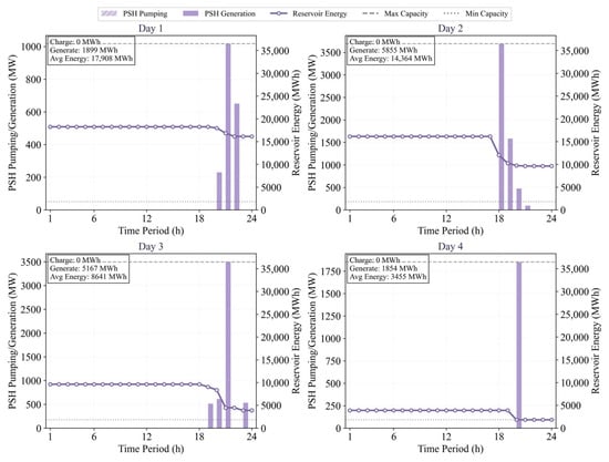
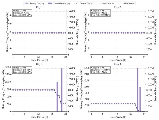
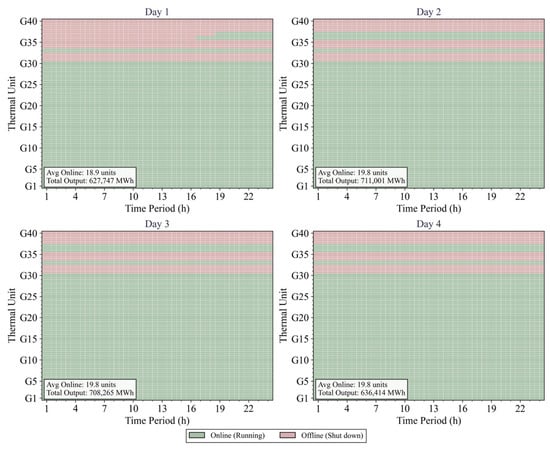
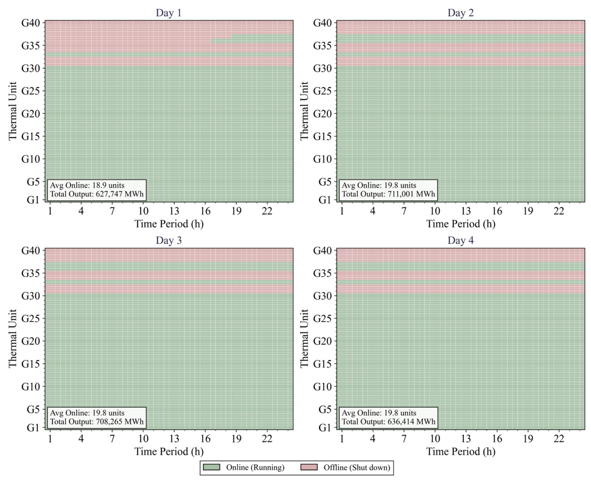
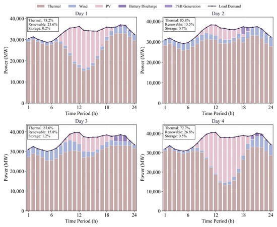
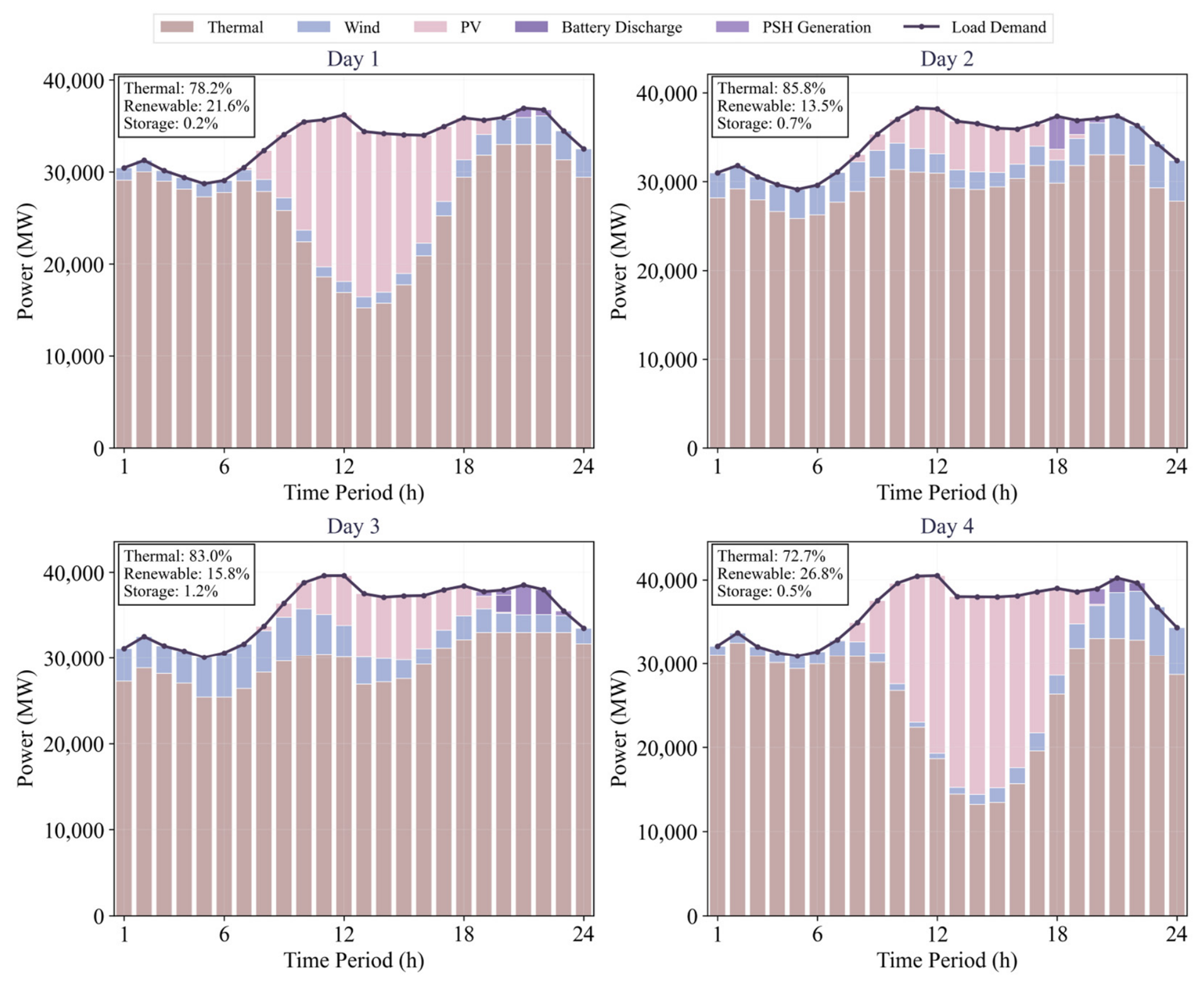
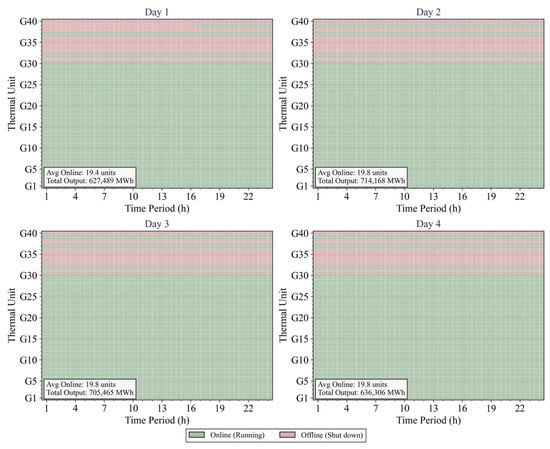
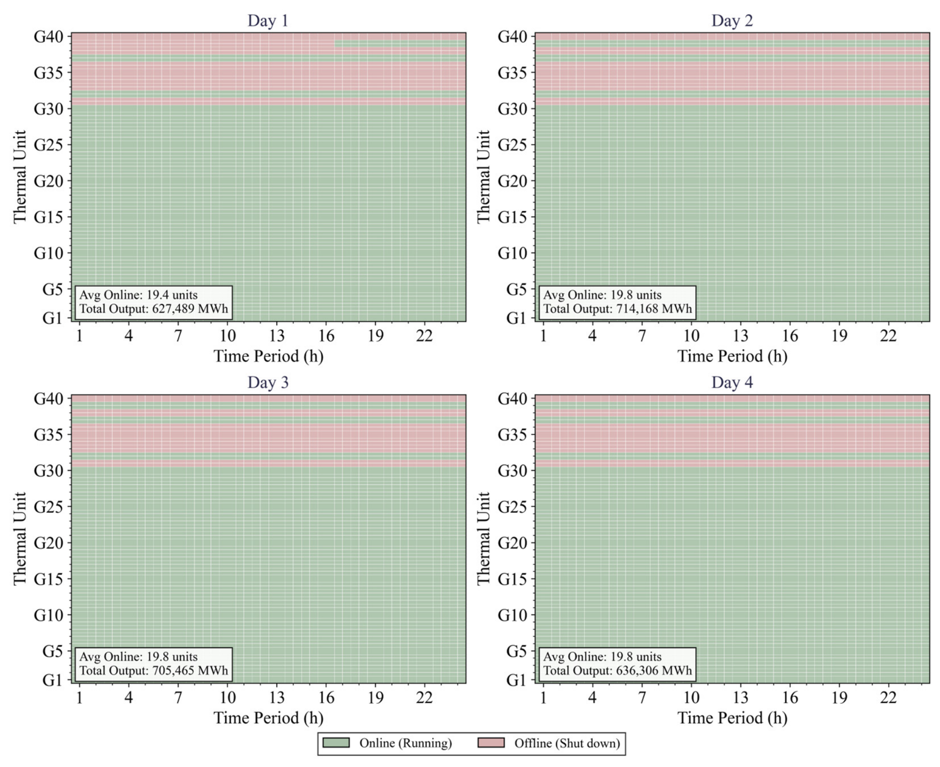
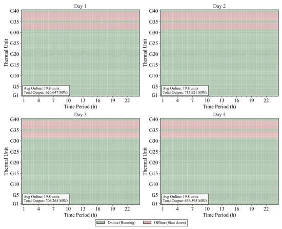
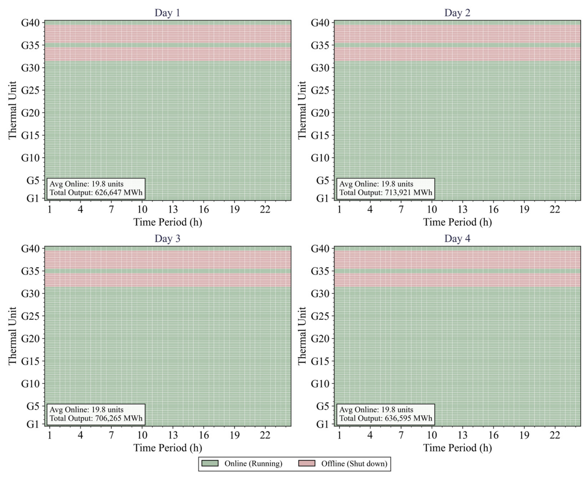
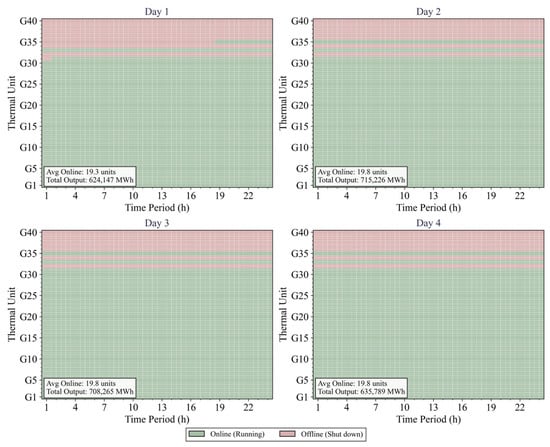
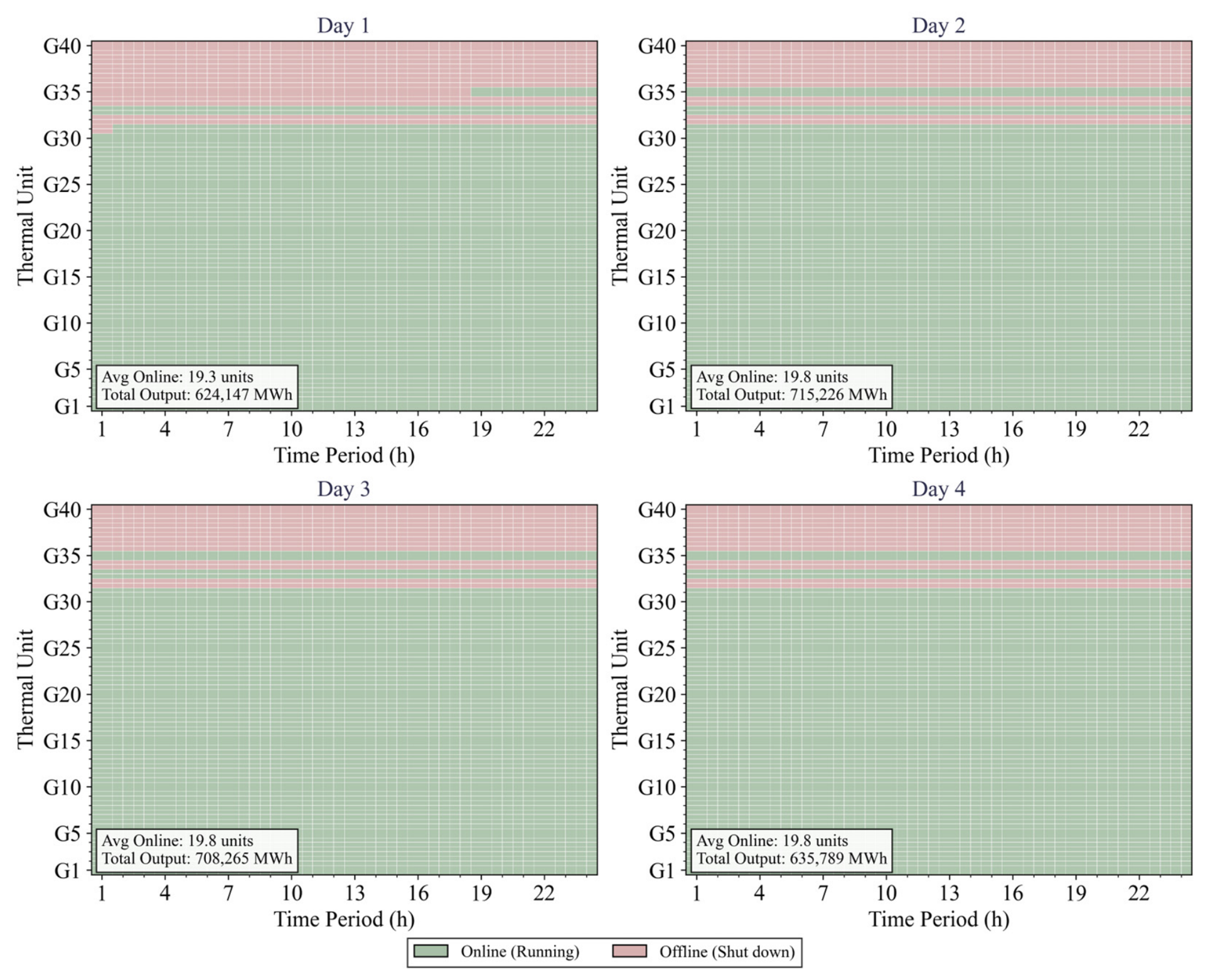
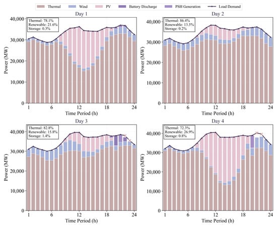
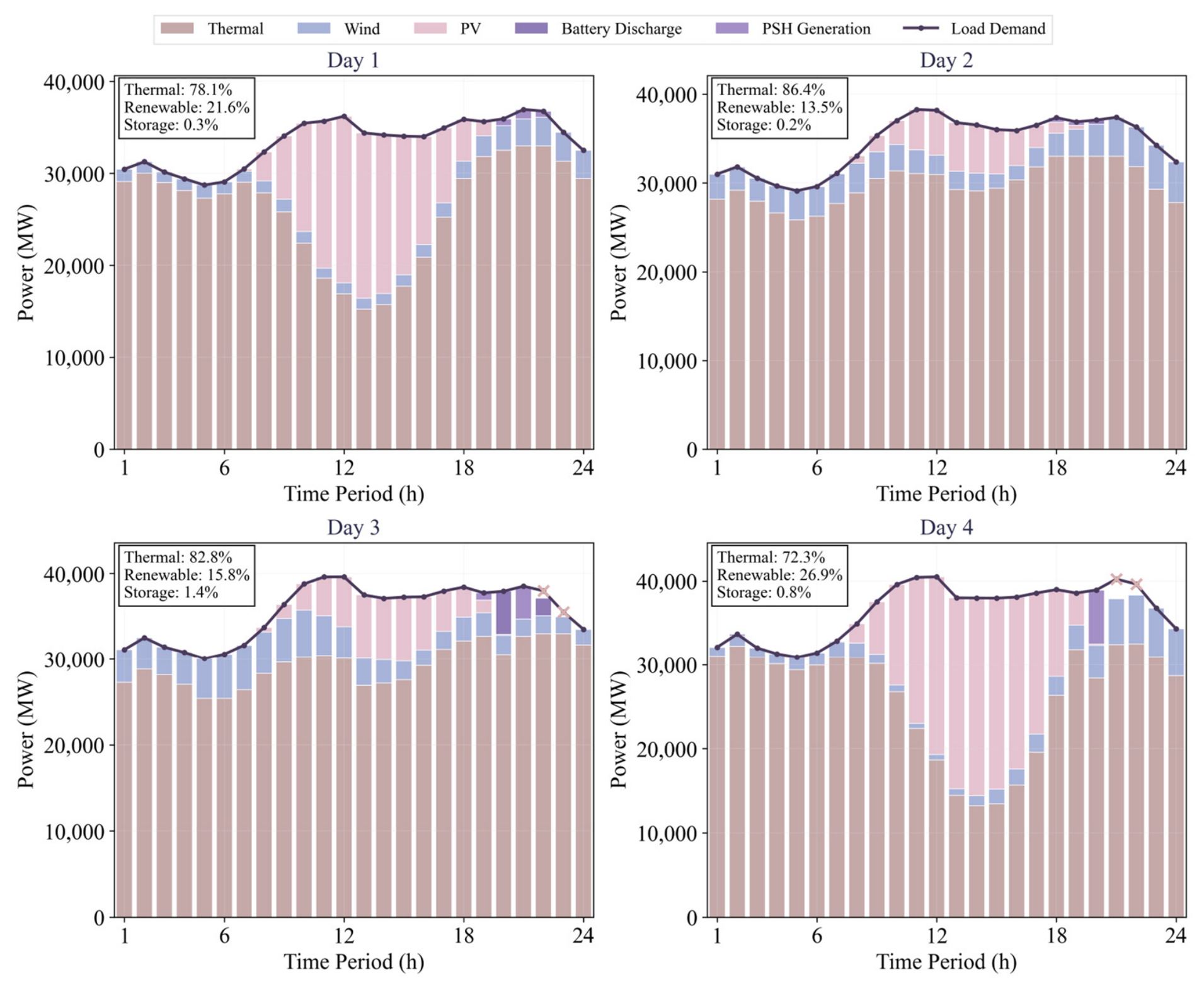

Disclaimer/Publisher’s Note: The statements, opinions and data contained in all publications are solely those of the individual author(s) and contributor(s) and not of MDPI and/or the editor(s). MDPI and/or the editor(s) disclaim responsibility for any injury to people or property resulting from any ideas, methods, instructions or products referred to in the content. |
© 2026 by the authors. Licensee MDPI, Basel, Switzerland. This article is an open access article distributed under the terms and conditions of the Creative Commons Attribution (CC BY) license.