Article

Improved Dung Beetle Algorithm for Multi-Objective Environmental Economic Dispatch of Microgrid

1
Key Laboratory of Regional Multi-Energy System Integration and Control, Shenyang Institute of Engineering, Shenyang 110136, China
2
Graduate School, Shenyang Institute of Engineering, Shenyang 110136, China
3
College of Automation, Shenyang Institute of Engineering, Shenyang 110136, China
*
Author to whom correspondence should be addressed.
Energies 2026, 19(13), 3206; https://doi.org/10.3390/en19133206
Submission received: 9 June 2026 / Revised: 25 June 2026 / Accepted: 29 June 2026 / Published: 6 July 2026

Abstract

With the widespread integration of renewable energy, microgrid environmental economic dispatch (EED) faces challenges such as uncertainties in wind and solar power outputs and multi-objective conflicts. This paper proposes a stochastic expected dispatch framework based on an improved multi-objective dung beetle optimization algorithm (MO-CLDBO). First, considering both wind–solar uncertainties and demand response, a Gaussian Copula function is employed to characterize the 24-h temporal correlations among wind speed, solar irradiance, and load, and typical scenarios are generated via Monte Carlo sampling and simultaneous backward reduction; a time-of-use demand response model is also introduced. Second, taking expected operational cost and environmental emission as dual objectives, three improvements are proposed to address the issues of uneven initial population, easy local convergence, and Pareto front collapse in the standard dung beetle algorithm: a Folded Two-Dimensional Modified Coupled Logistic-Sine Map (Folded 2D-MCLSM) is used to initialize a high-quality population, a non-dominated sorting mechanism is introduced, and a dynamic lens imaging backward learning strategy is designed. Finally, the proposed algorithm is compared with several classical algorithms in the mathematical model of microgrid optimal dispatch through 50 independent runs. Experimental results show that the improved dung beetle optimization algorithm achieves not only the lowest average operating cost, but also the best hypervolume (HV) indicator, demonstrating excellent comprehensive performance in multi-objective search convergence and solution set diversity.

1. Introduction

With the low-carbon transformation of the global energy structure and the further advancement of the “dual carbon” strategy, the large-scale integration of high-penetration distributed renewable energy (e.g., wind power and photovoltaics) into the grid has become a core feature of modern power systems [1,2,3]. According to official statistics, China’s total installed capacity of wind and photovoltaic power exceeded 1.84 billion kW by the end of 2025, accounting for more than 47.3% of the national total installed power generation capacity [4]. Northwest China, represented by Xinjiang, Inner Mongolia, Gansu, Qinghai, and Tibet (with Lhasa as the core load center), is endowed with superior wind and solar energy resources and has become the core cluster of China’s large-scale renewable energy bases. The combined installed capacity of wind and PV in the above five provinces accounts for over 40% of the national total, forming a distinct spatial pattern of “power generation in the west and load consumption in the east”.
To address the spatial mismatch between energy bases and load centers, China has built the world’s largest ultra-high voltage direct current (UHVDC) transmission network [5]. At present, dozens of ±800 kV UHVDC projects have been put into operation, and the world’s first ±1100 kV UHVDC transmission project has achieved large-capacity, long-distance cross-regional power transmission across 3300 km [6]. Meanwhile, research and engineering planning for ±1500 kV next-generation UHVDC technology are also advancing steadily, which will further improve the transmission capacity and economic efficiency of cross-regional energy allocation. Nevertheless, UHVDC transmission mainly addresses the large-scale outward power delivery from centralized renewable energy bases; for distributed renewable energy and terminal load clusters widely distributed in load centers, relying solely on long-distance transmission will lead to excessive line losses and insufficient operational flexibility. As a local integration carrier for distributed generation, multi-type energy storage systems, and flexible end-user loads, the microgrid plays a key supporting role in improving clean energy utilization efficiency and grid resilience [7]. In addition, with the liberalization of the retail electricity market, prosumer-oriented operation planning is of great significance for optimizing microgrid–grid interaction and BESS operation [8]. However, the strong randomness of renewable energy output and the dynamic fluctuations on the demand side pose severe technical challenges to the day-ahead operation scheduling of microgrids. Therefore, how to coordinate the output of heterogeneous distributed generation units while ensuring real-time power balance and achieve bilateral synergistic optimization of comprehensive economic cost and pollutant emissions remains a core scientific problem to be solved in the field of microgrid environmental economic dispatch (EED) [9,10,11].
Microgrid EED is essentially a typical high-dimensional, nonlinear, strongly constrained multi-objective optimization problem. At a fundamental level, wind speed and solar irradiance are governed by complex meteorological processes, exhibiting pronounced diurnal, seasonal, and interannual variations. In power system planning and baseline scheme design, typical meteorological year (TMY) data—screened from 10- to 30-year long-term observation series—are widely used to construct operation scenarios that reflect long-term average climatic conditions. However, TMY inherently filters out extreme meteorological events and interannual fluctuation features by selecting representative months, making it inadequate for supporting the refined operation of high-renewable-penetration distribution networks.
In contrast, complete long-term meteorological series offer great potential for the operation of such networks. First, they provide a full-sample data foundation for stochastic optimal dispatch: long-term series retain multi-scale statistical laws of meteorological elements, which support the construction of more realistic uncertainty models, enabling generated scenarios to cover both normal and extreme fluctuation conditions, thus effectively enhancing the robustness of day-ahead dispatch schemes. Second, they support extreme-risk identification and response: typical extreme scenarios—such as consecutive low-radiation days, prolonged wind lulls, and rapid wind ramp events—can be extracted from long-term meteorological records to guide spinning reserve configuration and emergency operation strategies, thereby mitigating operational risks caused by renewable energy fluctuations. Third, they enable multi-time-scale coordination: long-term series contain fluctuation information from interannual to intra-day levels, which can support medium- and long-term operation planning, seasonal storage scheduling, and the linkage between day-ahead and real-time dispatch, improving the overall economic efficiency of distribution networks.
To effectively translate these long-term profiles into reliable dispatch strategies, however, traditional deterministic day-ahead models must be re-evaluated, as they often fail to capture severe power imbalances and operational risks [12,13]. To tackle this issue, researchers have increasingly introduced scenario generation and stochastic programming techniques to quantify the uncertainties on both the supply and demand sides [14]. However, early studies mostly adopted single-variable probability distribution assumptions, which are often based on the strict premise that random variables are independent of each other, thereby neglecting the multi-dimensional spatiotemporal coupling characteristics among wind power, photovoltaic generation, and local load within the same geographical region over time. To more accurately capture such spatiotemporal dependencies, recent studies have gradually introduced Copula functions (e.g., Frank Copula or Gaussian Copula) to construct multivariate joint probability distributions [15,16,17]. Compared with traditional methods, Copula theory, by separating marginal distributions from correlation structures, can generate day-ahead typical operation scenarios that are more consistent with the physical reality of microgrids [18]. Building upon this, the present study constructs its Gaussian Copula modeling framework based on historical meteorological and load series, fully exploiting the temporal correlation information contained in the historical data. Through scenario generation and reduction techniques, this framework achieves the high-fidelity reproduction of wind–solar–load fluctuation characteristics.
On the other hand, under extreme scheduling scenarios with drastic fluctuations in wind and solar power output, relying solely on the flexible regulation of conventional gas turbines or diesel generators on the supply side is often constrained by their ramp rates, making it difficult to maintain real-time power balance on their own [19]. Therefore, introducing demand response (DR) on the load side, especially price-based demand response (PBDR) driven by time-of-use pricing signals, has become a key means of smoothing source–load fluctuations in microgrids by guiding users to shift electricity consumption away from peak hours [20,21]. However, existing models for constructing PBDR mechanisms often rely on static price elasticity matrices, generally neglecting the physical ramp limits of end-use loads during inter-temporal load shifting and the effect of user fatigue decay over time [22,23,24]. In practical engineering, such simplified linear modeling can easily lead to a systemic “rebound peak” due to the excessive load concentration shifted to low-price periods [25,26], thus significantly undermining the physical feasibility of optimal scheduling schemes.
At the algorithmic solving level, the high-dimensional, non-convex, and discontinuous characteristics of the microgrid EED problem render traditional gradient-based mathematical programming methods prone to failure when dealing with complex multi-objective frontiers [27]. Metaheuristic swarm intelligence algorithms, represented by the fast non-dominated sorting genetic algorithm (NSGA-II) [28] and the multi-objective particle swarm optimization algorithm (MOPSO) [29], have become the tools of choice for solving multi-objective day-ahead dispatch due to their independence from gradient information and strong global search capabilities. The dung beetle optimizer (DBO), a novel bio-inspired algorithm proposed by Xue and Shen in 2023, has demonstrated excellent convergence accuracy in engineering optimization owing to its unique multi-modal behavior mechanisms such as rolling, breeding, and foraging [30]. However, when the standard DBO is extended to a multi-objective optimization framework and faces high-dimensional microgrid dispatch models involving the complex temporal coupling of energy storage, it still suffers from poor spatial ergodicity of the initial population and a tendency to fall into specific local optima in the later stages of iteration. More importantly, when traditional non-dominated sorting handles high-dimensional conflicting objectives (e.g., the trade-off between economy and environmental protection) without an effective population diversity preservation mechanism to guide the search, the population is prone to excessive aggregation toward specific local extreme regions of the Pareto front. This significant drawback in multi-objective optimization, known as “Pareto front collapse”, prevents the algorithm from providing decision-makers with widely and evenly distributed flexible dispatch alternatives.
To address the above shortcomings, this paper constructs a multi-objective environmental economic dispatch model for microgrids that accounts for the spatiotemporal dependence of wind and solar power and refined demand response, and proposes an improved multi-objective dung beetle optimization algorithm (MO-CLDBO). The core innovative work of this paper is mainly reflected in the following three aspects:
  • Deep improvement of algorithm mechanism: A Folded Two-Dimensional Modified Coupled Logistic-Sine Map (Folded 2D-MCLSM) is constructed to replace pseudo-random numbers for enhancing the quality of the initial population; a fast non-dominated sorting and crowding distance mechanism is integrated; and a dynamic lens imaging backward learning (DLIBL) strategy is designed to provide strong momentum for the population to escape from non-convex local deadlocks.
  • Characterization of spatiotemporal dependence uncertainty: A multivariate joint probability model of wind speed and solar irradiance is established using the Gaussian Copula function, coupled with Monte Carlo sampling and simultaneous backward reduction for typical scenario reduction, closely restoring the physical temporal characteristics.
  • Model engineering refinement and validation: A PBDR model incorporating a time decay factor and transfer ramp constraints is introduced. Simulation results demonstrate that MO-CLDBO achieved the best performance in both the comprehensive hypervolume (HV) indicator and emission reduction benefit assessment, and passed the Wilcoxon rank-sum test.
It is worth emphasizing that the novelty of this paper does not stem from the use of non-dominated sorting, chaotic maps, or opposition-based learning per se, but rather from: (i) the specific mathematical improvements made to the chaotic map (the folded 2D-MCLSM with a modulo folding operator) and the opposition-based learning strategy (DLIBL with dynamic target-guided adaptation); (ii) their synergistic integration into a unified multi-objective optimization framework (MO-CLDBO); and (iii) the application of this enhanced algorithm to a comprehensive microgrid environmental economic dispatch model that explicitly incorporates spatiotemporal correlations and refined demand response. By coordinating these interdependent elements, this work offers a potential alternative for alleviating certain algorithmic and engineering challenges that conventional stochastic dispatch models may struggle to fully conquer. These three interconnected aspects collectively constitute the original contributions of this work.

2. Microgrid Operation Structure

The day-ahead multi-objective dispatch system for microgrids constructed in this paper encompasses distributed renewable energy (wind turbine, WT; photovoltaic, PV), controllable generation units (micro gas turbine, MT; diesel generator, DG), a battery energy storage system (BESS), as well as flexible end-user loads participating in price-based demand response (PBDR). The system enables bidirectional power exchange via the grid connection line. The core objective of dispatch is to optimize the power output of each controllable unit over a 24-h scheduling horizon while satisfying multiple stringent physical constraints, thereby achieving an optimal trade-off between comprehensive operating costs and pollutant emissions.

2.1. Basic Structure of Microgrid

2.1.1. Photovoltaic Array

The photovoltaic output is closely related to solar irradiance and ambient temperature. This paper adopts an engineering practical model, and its output power is given by:
P PV ( t ) = P STC G ( t ) G STC [ 1 + α T ( T ( t ) T STC ) ]
where P STC is the rated power of the photovoltaic module under standard test conditions (kW), G ( t ) is the actual solar irradiance (W/m2), G STC is the solar irradiance under standard test conditions (W/m2), α T is the temperature coefficient (/°C), T ( t ) is the panel temperature (°C), and T STC is the temperature of the photovoltaic module under standard test conditions (°C, typically 25). It is worth noting that the photoelectric conversion efficiency of the PV module is inherently integrated into the rated power parameter PSTC under standard test conditions.

2.1.2. Wind Turbine

Wind energy is another major source of renewable energy. The mathematical model of wind turbine output power can be expressed as:
P W T = { 0 , v h u b < v c i   or   v h u b > v c o v h u b v c i v N v c i P N , v c i v h u b v N P N , v N < v h u b v c o
In the formula, v ci , v N , v co are the cut-in wind speed, rated wind speed, and cut-out wind speed, respectively (m/s), and P N is the rated power (kW).

2.1.3. Micro Gas Turbine

Micro gas turbines are small, efficient distributed generation units, typically with a single-unit power output ranging from 25 kW to 500 kW. The operating efficiency of a micro gas turbine is given as follows:
η M T = 0.0753 [ P M T ( t ) 65 ] 3 0.3095 [ P M T ( t ) 65 ] 2 + 0.4174 [ P M T ( t ) 65 ] + 0.1068
Among them, η M T is the operating efficiency of the micro gas turbine, and P MT ( t ) is the active power output of the micro gas turbine (kW). The fuel cost of the gas turbine can be expressed as follows:
C M T = C L H V η M T ( t ) P M T ( t )
Operation and maintenance cost is expressed as:
C M T , o m = K M T . o m P M T ( t )
In the formula, P MT is the output power of the micro gas turbine (kW), η MT is the efficiency of the micro gas turbine, LHV is the low heating value (kWh/m3), C is the natural gas price (fixed at 2.5 CNY/m3), and K MT is the maintenance coefficient of the micro gas turbine (CNY/kWh).

2.1.4. Diesel Generator

In the microgrid architecture with an increasing share of clean energy, retaining an appropriate number of diesel generators as backup units is an important strategy for balancing power supply stability and transitional economy. Their fuel cost is a quadratic function:
C D G ( t ) = a P D G 2 ( t ) + b P D G ( t ) + c
Operation and maintenance cost is expressed as:
C D G , o m ( t ) = K D G , o m P D G ( t )
where C DG ( t ) and C DG , om ( t ) are the fuel cost and operation (CNY) and maintenance cost of the diesel generator at time t , respectively; P DG ( t ) is the power generation of the diesel generator at time t ; K DG , om is the operation and maintenance cost coefficient of the diesel generator (CNY/kWh); and a (CNY/kW2·h), b (CNY/kW.h), c (CNY/h) are the coefficients of the diesel generator.

2.1.5. Energy Storage System

The energy storage system is used for peak shaving and valley filling as well as power balancing. The mathematical expression of its state of charge (SOC) is given as follows:
S O C ( t ) = { S O C ( t 1 ) P E S S ( t ) Δ t η d i s E m a x , P E S S ( t ) > 0 S O C ( t 1 ) P E S S ( t ) η c h Δ t E m a x , P E S S ( t ) 0
where P ESS ( t ) > 0 represents discharging, P ESS ( t ) < 0 represents charging, η ch and η dis are the charging and discharging efficiencies, and E max is the maximum capacity of the energy storage system (kWh).

2.1.6. Interaction with Main Grid

In the grid-connected operation mode, the microgrid can perform bidirectional power exchange with the main grid. The corresponding grid interaction cost is given as follows:
C g r i d ( t ) = { c b u y ( t ) P g r i d ( t ) , P g r i d ( t ) > 0 c s e l l ( t ) P g r i d ( t ) , P g r i d ( t ) 0
where P grid ( t ) > 0 indicates electricity purchase, P grid ( t ) < 0 indicates electricity sale, the purchase price is c buy ( t ) (CNY/kWh), and the sale price is c sell ( t ) (CNY/kWh).

2.2. Demand Response Model

Price-based demand response (PBDR) actively guides users to adjust their electricity consumption behavior through price signals by formulating a reasonable time-of-use (TOU) pricing strategy, thereby achieving the peak load shifting and valley filling of microgrid loads. According to the price elasticity of demand theory in microeconomics, the rate of change in load is positively correlated with the rate of change in electricity price. This paper quantifies this response characteristic by constructing a price elasticity matrix E :
E = [ E 1,1 E 1,2 E 1,24 E 2,1 E 2,2 E 2,24 E 24,1 E 24,2 E 24,24 ]
E ( i , j ) = Δ L ( i ) / L 0 ( i ) Δ p ( j ) / p 0
In the formula, Eij is the elasticity coefficient at the i -th row and j -th column, representing the percentage change in load at time i in response to a percentage change in electricity price at time j . L 0 ( i ) is the initial load at time i (kW), and Δ L ( i ) is the load change at time i (kW); Δ p ( j ) is the electricity price change at time j (CNY/kWh), and p 0 is the base electricity price (CNY/kWh). When i = j , the coefficient is the self-elasticity (typically negative); when i j , it is the cross-elasticity (typically positive).
Traditional PBDR models usually assume that users can shift loads without any restrictions to any time period. However, in practical engineering, users’ willingness to shift loads significantly decays as the time span increases. To address this, this paper constructed a cross-elasticity coefficient model that accounts for time-coupled decay:
E ( i , j ) = ε e x p ( γ m i n ( | i j | , 24 | i j | ) ) ( i j )
In the formula, ε is the base cross-elasticity coefficient; γ is the time decay factor (h−1, taken as 0.15 in this paper); the min function in the formula perfectly accommodates the circular time characteristic of the 24-h operation scheduling of the microgrid.
Based on the above elasticity matrix, the preliminary response load L DR after implementing PBDR is calculated as follows:
L D R ( t ) = L 0 ( t ) [ 1 + j = 1 24 E ( t , j ) Δ p ( j ) p 0 ]
In the formula, L D R ( t ) is the preliminary response load at time t after implementing PBDR (kW), and Δ p ( j ) is the electricity price change at time j (CNY/kWh).
To ensure physical feasibility and prevent rebound peaks, the following constraints are imposed on the load adjustment:
Ramp constraint for rebound peak prevention: The hourly load variation is limited to avoid secondary peaks:
| L D R ( t ) L D R ( t 1 ) | 0.10 L ˉ 0 , t [ 2,24 ]
where L ˉ 0 is the daily average load. The same limit applies between t = 24 and t = 1 to ensure smooth transition across the daily boundary. This constraint explicitly enforces the claimed transfer ramp limit [31].
Load transfer limit: The hourly load adjustment is capped to prevent excessive shifting:
| L D R ( t ) L 0 ( t ) | 0.15 L 0 ( t )
This reflects the practical reality that only flexible loads can participate in DR, while rigid loads remain unchanged.
Circular boundary constraint: The same ramp limit applies across the daily boundary:
| L D R ( 1 ) L D R ( 24 ) | 0.10 L ˉ 0
This ensures smooth load transition between the end and the beginning of the 24-h horizon.
Total daily energy conservation is not strictly enforced, as price signals may induce genuine conservation rather than pure load shifting; excessive deviations are penalized via C DR . Only shiftable loads participate, enforced by the 15% hourly cap, while rigid loads remain unchanged. The compensation coefficient C comp = 0.12 (CNY/kWh) is calibrated based on typical DR programs, where incentive rates generally range from 0.10 to 0.20 (CNY/kWh) [32].
In the proposed PBDR model, several practical considerations are addressed. First, user comfort is respected by capping hourly load adjustments at 15% of the original load, preventing excessive disruption to consumption patterns. Second, the ramp rate constraint—limiting hourly load variations to 10% of the daily average load—mitigates the load rebound effect, i.e., the formation of secondary peaks when curtailed loads are recovered during adjacent off-peak periods [33]. Third, following the load classification scheme in [34,35], only shiftable loads participate in load shifting, while rigid loads remain unchanged. Fourth, the time decay factor γ = 0.15 quantifies the decay of users’ willingness to shift load with time separation—each additional hour reduces the cross-elasticity coefficient by approximately 13.9%, reflecting behavioral resistance to temporally distant adjustments. Finally, the model adopts standard assumptions including price-taking behavior, rational economic response, and homogeneous user characteristics, consistent with common PBDR practices [33,35].

3. Multi-Objective Optimization Model of Microgrid

3.1. Objective Function

Microgrid dispatch pursues two conflicting objectives: minimizing the expected economic cost and minimizing the expected environmental emission.

3.1.1. Expected Economic Cost

The first objective function F 1 represents the comprehensive expected operating cost of the system under K typical scenarios. This cost covers the fuel cost of micro gas turbines and diesel generators, equipment operation and maintenance costs, power exchange cost with the main grid, demand response compensation cost, and the physical violation penalty cost triggered by extreme power imbalance. Its mathematical expression is given as follows:
F 1 = k = 1 K π k ( C g e n , k + C O M , k + C g r i d , k + C p e n , k + C D R , k )
where K is the total number of typical scenarios after simultaneous backward reduction; π k is the occurrence probability of the k -th typical scenario; C gen , k is the comprehensive fuel cost of power generation (CNY); C OM , k is the equipment operation and maintenance cost (CNY); C grid , k is the grid interaction cost (CNY); C DR , k is the demand response compensation cost (CNY); and C pen , k is the physical violation penalty cost (CNY).
The power generation fuel cost C gen , k (CNY) is divided into the fuel cost of micro gas turbines C MT , k (CNY) and the fuel cost of diesel generators C DG , k (CNY), expressed as follows:
C g e n , k = C M T , k + C D G , k
{ t = 1 T i = 1 N M T c L H V η M T ( t ) P M T ( t ) t = 1 T j = 1 N D G a D G , j P D G , j , t 2 + b D G , j P D G , j , t + c D G , j
In the formula, T is the dispatch period, set to 24 h; N MT and N DG are the numbers of MT and DG units, respectively, P MT ( t ) and P DG ( t ) are the output powers (kW), and a DG , j (CNY/kW2), b DG , j (CNY/kW), and c DG , j (CNY) are the cost coefficients for the diesel generators.
The equipment operation and maintenance cost C OM , k (CNY) includes the wear and depreciation expenses of all distributed power sources and the energy storage system during the operation period:
C O M , k = t = 1 T ( K M T P M T , t + K D G P D G , t + K P V P P V , t + K W T P W T , t + K E S S | P E S S , t | )
In the formula, K is the unit operation and maintenance cost coefficient of each corresponding device (CNY/kWh).
The grid interaction cost C grid , k (CNY) represents the electricity purchase and sale expenses when the microgrid exchanges power with the external grid:
C g r i d , k = t = 1 T P g r i d , t ( c b u y ( t ) I b u y + c s e l l ( t ) I s e l l )
In the formula, P grid , t is the power transmitted through the tie line (kW), with positive values indicating electricity purchase by the microgrid and negative values indicating electricity sale; c buy ( t ) and c sell ( t ) are the time-of-use purchase and sale prices, respectively (CNY/kWh); and I buy and I sell represent the status of electricity purchase and sale.
The demand response compensation cost C DR , k (CNY) is the economic incentive issued by the microgrid dispatch center to users participating in load shifting:
C D R , k = t = 1 T C c o m p | P L o a d , t k P L o a d , o r i g , t k |
In the formula, C comp is the unit compensation price per unit of transmitted power (CNY/kWh), which is 0.15 CNY/kWh; P Load , t k and P Load , orig , t k are the load power after and before the demand response, respectively (kW).
The physical violation penalty cost is C pen , k (CNY). When the tie-line power exchange reaches its upper limit and still cannot satisfy the supply–demand balance, the system will forcibly shed load or curtail wind and solar power, resulting in penalties for load loss and power curtailment:
C p e n , k = t = 1 T ( λ l o s s P l o s s , t + λ c u r t a i l P c u r t a i l , t )
In the formula, λ l o s s (CNY/kWh) and λ curtail (CNY/kWh) are the unit penalty coefficients for load shedding and wind/solar power curtailment, respectively.

3.1.2. Minimization of Expected Environmental Emissions

The second objective function F 2 (kg) aims to reduce the emissions of greenhouse gases (CO2) and pollutant gases (NOₓ) released into the atmosphere during microgrid operation:
F 2 = k = 1 K π k t = 1 T [ E M T P M T , t + E D G P D G , t + E g r i d P g r i d , t b u y + E p e n P l o s s , t ]
In the formula, E MT (g/kWh), E DG (g/kWh), and E grid (g/kWh) are the comprehensive pollutant emission factors for the micro gas turbine, diesel generator, and power purchased from the main grid, respectively; E pen (kg/kWh) is the indirect social and environmental penalty equivalent caused by forced load shedding. Note that the emission factors for MT, DG, and the grid adopt the unit of g/kWh, while the final total emission F 2 is obtained by summing the weighted contributions and converting the result into kilograms (kg) by dividing by 1000.

3.2. Operation Constraints

To ensure the safe and stable operation of the microgrid under complex operating conditions, the solution of the above objective functions must strictly satisfy the following physical constraints.

3.2.1. Power Balance Constraint

In any scenario and at any time period, the total power supply within the microgrid must maintain real-time balance with the load after demand response:
i = 1 N M T P M T , i , t + j = 1 N D G P D G , j , t + P P V , t + P W T , t + P g r i d , t + P E S S , t = P L o a d , t
It should be noted that in this paper, it is stipulated that P ESS , t > 0 when the energy storage system is discharging, and P ESS , t < 0 when it is charging.

3.2.2. Unit Output Bound and Ramp Rate Constraints

The output power of conventional controllable units must be limited by their rated capacity, and the ramp rates of power changes between adjacent time periods are constrained by mechanical performance.
P i m i n ( t ) P i ( t ) P i m a x ( t )
D R i P i ( t ) P i ( t 1 ) U R i
In the formula, P i m i n and P i m a x are the minimum and maximum technical output of the i -th unit, respectively (kW); D R i and U R i are its maximum downward and upward ramp rates, respectively (kW/h).

3.2.3. Operation Constraints of Energy Storage System

The state of charge (SOC) of the battery energy storage system exhibits time-coupled characteristics. Its charging and discharging behavior must satisfy capacity limits and ensure energy balance at the beginning and end of the dispatch period to maintain the capacity for cyclic operation on the following day:
S O C m i n S O C ( t ) S O C m a x
S O C ( 24 ) = S O C ( 0 ) = S O C i n i t
Among them, S O C m i n and S O C m a x are the allowable extreme values of the state of charge; S O C init is the initial value of the state of charge set by the system at the beginning and end of the dispatch period.

3.2.4. Tie-Line Power Exchange Constraints

The tie-line power exchange constraint is expressed as:
P g r i d m i n ( t ) P g r i d ( t ) P g r i d m a x ( t )
In the formula, P g r i d m i n ( t ) is the lower physical capacity limit of the tie line connecting to the main grid (kW); P g r i d m a x ( t ) is the upper physical capacity limit of the tie line connecting to the main grid (kW).

3.2.5. Constraint Handling Strategy

A hybrid constraint-handling strategy is implemented to ensure the physical viability of the solutions. For hard constraints—including generation capacity limits, ramp-rate boundaries, and state of charge (SOC) limits—infeasible solutions are directly repaired by clamping variables to their permissible operational ranges and adaptively adjusting the battery charging/discharging profiles. Crucially, a terminal constraint is enforced to force the SOC back to its initial state at the end of the 24-h scheduling horizon. Conversely, soft constraints—encompassing power balance and tie-line exchange limits—are managed by incorporating penalty costs into the multi-objective fitness function. Specifically, the penalty coefficients are configured as 50 CNY/kWh for load shedding and 20 CNY/kWh for renewable curtailment, coupled with an additional environmental penalty of 1.5 kg/kWh for load shedding events.

3.3. Wind and PV Uncertainties

The uncertainty model is constructed from one-year hourly data (wind speed, solar irradiance, and load), reshaped into daily 24-h profiles. The data are preprocessed through standard procedures including outlier filtering and reshaping into daily profiles. Marginal distributions are fitted using the empirical cumulative distribution function for wind speed (to avoid parametric bias), the beta distribution for solar irradiance, and the normal distribution for load. The Gaussian Copula correlation matrix is estimated via maximum likelihood. Load uncertainty is explicitly included in the joint distribution, and its statistical fidelity is validated in Section 5.2.1.

3.3.1. Gaussian Copula Joint Distribution

To capture the temporal correlations among wind speed, solar irradiance, and load (including multivariate correlations at the same time slice and autocorrelations of the same variable at different time instants), this paper introduces the Gaussian Copula.
Let U = [ U 1 , U 2 , , U d ] be the vector of uniform distributions obtained from each random variable through probability integral transformation, where d = 24 (wind speed) +   N solar (effective sunshine hours) +   24 (load). The joint cumulative distribution function of the Gaussian Copula is given by:
C ( u 1 , u 2 , , u d ; ρ ) = Φ R ( Φ 1 ( u 1 ) , Φ 1 ( u 2 ) , , Φ 1 ( u d ) )
In the formula, d is the total dimension; u d is the probability integral transformation value of the empirical marginal distribution for each variable; Φ R is the standard multivariate normal distribution function with correlation matrix ρ ; and Φ 1 is the inverse function of the standard normal distribution.

3.3.2. Mechanism of Characterizing Temporal Correlation via Gaussian Copula

The conventional independent probability distribution assumption forcibly disconnects the continuity of time series and the physical coupling between devices. Based on Sklar’s theorem, the Gaussian Copula function can map multiple random variables with different marginal distributions into a unified joint probability space without loss of information, thereby accurately separating and extracting the dependency structure among variables. In the model construction stage, historical meteorological and load data are first reconstructed into a high-dimensional time series matrix according to daily characteristics. To avoid truncation errors caused by prior parametric assumptions, the wind speed sequence adopts a nonparametric empirical cumulative distribution function (Empirical CDF) to directly extract marginal distributions through sample ranks; the solar irradiance and load sequences are fitted using the beta distribution and normal distribution, respectively.
To address the issues of “zero-value stacking” in high-dimensional joint distributions and covariance matrix singularity caused by the zero output of photovoltaics at night, a dynamic physical dimensionality reduction mechanism is introduced. By removing ineffective radiation periods at night, the dimension of the dependency structure is compressed. The reduced effective time series are mapped to the standard uniform distribution domain through probability integral transformation, and then substituted into the Gaussian Copula function to solve the correlation matrix ρ . This matrix mathematically and accurately captures the nonlinear dependencies and fluctuation coupling characteristics of wind, solar, and load at 24 daily time nodes.
In addition, t-Copula, vine Copula, and KDE-Copula were considered but not adopted due to their high computational cost in high-dimensional settings, complex parameter estimation, or limited scalability. The Gaussian Copula strikes a favorable balance between modeling fidelity and computational tractability for the day-ahead dispatch problem considered in this study.

3.3.3. Monte Carlo Sampling and Synchronous Backward Reduction

Based on the Gaussian Copula joint probability model that incorporates the real temporal correlations described above, the generation and refinement process of uncertainty scenarios is carried out in two stages:
Stage 1: Large-scale generation of dependent scenarios. Monte Carlo sampling (MCS) is used to generate a large number (set to 1000 groups) of initial joint random samples in the standard uniform distribution domain. Subsequently, the inverse cumulative distribution functions of each variable (e.g., quantile inverse mapping for wind speed, beta inverse transform for solar irradiance) are applied to map the uniform distribution samples back into actual physical power time series. At the end of the inverse mapping, absolute extreme value clamping is applied to the generated physical sequences to filter out violation distortion data caused by tail divergence.
Stage 2: Simultaneous backward reduction (SBR): To avoid the curse of dimensionality, the SBR algorithm reduces the initial scenario set. Guided by the Kantorovich distance, it uses the Euclidean distance as the transport cost. At each iteration, the scenario with the smallest probability-weighted distance to its nearest neighbor is removed, and its probability is transferred to that neighbor. This procedure ensures minimal loss of the original probability distribution.
After multiple rounds of iterative backward reduction, the large set of scenarios is reduced to the set number K of discrete typical scenarios (set to 5 in this paper). This physical evolution process achieves a dimensionality reduction transformation from strong uncertainty to discrete deterministic scenarios and their corresponding occurrence probabilities π k , while preserving the original multivariate joint probability distribution characteristics and strict temporal dependency structures to the greatest extent possible.

4. Improved Multi-Objective Dung Beetle Optimizer

4.1. Dung Beetle Optimizer

The DBO algorithm simulates four main operational processes of dung beetles: rolling, breeding, foraging, and stealing, and finally selects the optimal solution.
(1) Ball-rolling dung beetles
During the rolling process, dung beetles use a celestial navigation mechanism to change their path, and their movement trajectory is influenced by both light source intensity and environmental disturbances.
{ x i ( t + 1 ) = x i ( t ) + a k x i ( t ) + b Δ x Δ x = | x i ( t ) X ω |
In the formula, t is the iteration number; x i ( t ) represents the position of the i -th dung beetle at the t -th iteration; k is a constant in the interval ( 0 , 0.2 ] ; b is a constant in the interval ( 0 , 1 ) ; a is an environmental disturbance coefficient taking the value 1 or 1 ; X ω is the global worst solution; and Δ x represents the change in light intensity.
(2) Breeding dung beetles
Female individuals select the optimal egg-laying area through a dynamic boundary strategy. The egg-laying area is dynamically adjusted with the number of iterations, and the position of the brood ball also changes dynamically accordingly.
B i ( t + 1 ) = X + b 1 ( B i ( t ) L b ) + b 2 ( B i ( t ) U b )
In the formula, B i ( t ) represents the position of the i -th brood ball at the t -th iteration; b 1 and b 2 are both 1 × D independent random vectors; D is the dimension of the optimization problem.
(3) Small dung beetles
The position update of small dung beetles during the foraging process is as follows:
x i ( t + 1 ) = x i ( t ) + C 1 ( x i ( t ) L b b ) + C 2 ( x i ( t ) U b b )
In the formula, C 1 is a random number following a normal distribution; C 2 is a random number in the interval ( 0 | 1 ) .
(4) Thieving dung beetles
Thieving dung beetles steal the dung balls of other dung beetles, and their position update method is as follows:
x i ( t + 1 ) = X b + S × g ( | x i ( t ) X * | + | x i ( t ) X b | )
In the formula, S is a constant representing the intensity of competition; g is a 1 × D random vector following a normal distribution.

4.2. Improvement Strategy 1: Two-Dimensional Modulus-Based Coupled Chaotic Map

In swarm intelligence optimization algorithms, the quality of the initial population directly determines the global exploration capability in the early stage and the convergence speed in the later stage. The standard DBO algorithm typically uses a pseudo-random number generator to uniformly distribute the initial population within a given solution space. However, when facing high-dimensional non-convex economic-environmental dispatch problems, conventional random initialization can easily lead to an uneven distribution of the population in the solution space, resulting in the clustering of individuals or blind spots in promising regions, causing the algorithm to fall into local optima at the early stage of iteration.
To achieve better ergodicity of the population, traditional algorithms often employ one-dimensional chaotic maps (such as the tent or logistic map). Nevertheless, under limited computer floating-point precision, one-dimensional maps are prone to falling into short-period orbits. Moreover, the topological projection characteristics of continuous chaotic maps determine that their probability density exhibits a typical “U-shaped” distribution, leading to severe accumulation of initial solutions at the boundaries of the multi-dimensional search space.
To address the above issues and achieve nearly complete ergodicity and unbiased distribution of the population, this paper proposes a two-dimensional coupling chaotic map based on the modulo operator, termed the Folded 2D Modified Coupled Logistic-Sine Map (Folded 2D-MCLSM). Unlike existing chaotic maps, Folded 2D-MCLSM adopts the modulo (mod) operation instead of the sine function as the boundary constraint mechanism, combined with a parameter amplification strategy. This allows the chaotic state to fully expand during iteration and then be folded back into a bounded interval via the modulo operation, thereby achieving two key advantages: First, complete ergodicity—the modulo operation fundamentally eliminates the distribution preference introduced by the sine function, enabling the chaotic sequence to cover the entire domain without gaps in the phase space. Second, highly uniform numerical distribution—the modulo folding operation breaks the nonlinear distortion caused by sine compression, ensuring that the output sequence maintains absolute uniformity in probability density. Its mathematical model is expressed as follows:
{ z x t + 1 = mod ( α z x t ( 1 z x t ) + β sin ( π z y t ) , 1 ) z y t + 1 = mod ( α z y t ( 1 z y t ) + β sin ( π z x t ) , 1 )
where z x t , z y t ( 0 , 1 ) are the chaotic state variables of the two dimensions, α and β are control parameters, and mod   ( , 1 ) denotes the fractional part operation. In this paper, α = β = 4 was chosen to maximize the complexity and ergodicity of the chaotic system.
Compared with the standard DBO algorithm, the MO-CLDBO algorithm using the two-dimensional coupled chaotic map based on the modulo operator achieves a more uniform distribution of initial solutions in the objective space, effectively reducing the probability of the initial population falling into local Pareto traps, thereby laying a solid foundation for subsequent efficient multi-objective optimization.

4.3. Improvement Strategy 2: Dynamic Lens Imaging Backward Learning (DLIBL)

In the middle and late stages of multi-objective microgrid dispatch iteration, the population tends to quickly converge toward the current non-dominated solution set (i.e., the local Pareto front). Due to the creation of a large number of local valleys in the high-dimensional solution space, the conventional DBO algorithm has strong exploitation capability near local extreme points but insufficient global escape ability to jump out of deep local traps. To address this issue, this paper introduces a dynamic lens imaging backward learning mechanism while retaining the non-dominated sorting framework.
(1) Mathematical model of dynamic lens imaging backward learning
The symmetry center of standard lens imaging backward learning is still the geometric center C of the search region. However, in the multi-objective economic-environmental dispatch of microgrids with complex nonlinear constraints, the geometric center often does not possess high-quality fitness information, leading to blindness in standard backward learning. The standard imaging formula can be expressed as:
X l e n s , j = l b j + u b j 2 + l b j + u b j 2 k X b e s t , j k
In this paper, the static optical center C of the lens is dynamically mapped to the Pareto-optimal individual X best with Rank-1 in the non-dominated sorting at each iteration, and the refracted object X is mapped to the inferior individual X worst with poor fitness. Substituting these into the above formula yields the dynamic target-guided refraction formula proposed in this paper:
X l e n s = X b e s t + X b e s t X w o r s t k
where k lens > 0 is called the lens adjustment coefficient.
(2) Design of dynamic adaptive mechanism
To perfectly match the search requirements of microgrid dispatch at different iteration stages, this paper adopts a dual dynamic nonlinear design for the trigger probability and the scaling factor k :
1. Nonlinear trigger probability P DLIBL
To avoid wasting computational resources and disrupting the converged excellent population by performing backward learning at every iteration, an intervention probability P DLIBL that decays nonlinearly with the number of iterations is introduced:
P D L I B L = e x p ( 5 ( t M ) 2 )
2. Dynamic scaling factor k
A fixed scaling factor cannot balance the broad exploration in the early stage and the deep exploitation in the later stage. This paper designs it as a variable that dynamically increases with the number of iterations:
k = 1 + 2 ( t M )
From the formula, it can be seen that in the early stage of iteration, the value of k is small, resulting in a larger refraction step size, which allows newly generated individuals to transition to emerging search regions farther from the optical center. As the iteration progresses, the value of k increases linearly, the refraction step size shortens, and the generated individuals will closely surround the Pareto optimal solution for refined fine-tuning.

4.4. Non-Dominated Sorting Mechanism

Multi-objective optimization problems are significantly different from single-objective ones. When multiple objectives exist, conflicts among them make it impossible to directly compare solutions, and thus it is difficult to find a single solution that simultaneously optimizes all objective functions. To address this issue, this paper introduces a non-dominated sorting mechanism to improve the selection process of the dung beetle algorithm. The non-dominated sorting mechanism originates from the non-dominated sorting genetic algorithm and performs well in high-complexity scenarios such as microgrid optimal dispatch.
(1) Definition of Pareto dominance relation
Let any two candidate solutions be x i and x j , and their corresponding objective function vectors be:
F ( x ) = [ f 1 ( x ) , f 2 ( x ) , , f M ( x ) ]
where M is the number of objective functions. For a minimization problem, if candidate solution x i is not worse than x j in all objectives and is strictly better than x j in at least one objective, then x i is said to dominate x j , denoted as x i x j . Its mathematical expression is:
{ f m ( x i ) f m ( x j ) , m = 1,2 , , M m , f m ( x i ) < f m ( x j )
Based on the above dominance relation, all individuals in the population can be divided into several non-overlapping non-dominated fronts. Among them, individuals in the first non-dominated front are not dominated by any other individuals in the population and possess the highest Pareto superiority; individuals in the second non-dominated front are only dominated by individuals in the first front, and so on. By stratifying the candidate solutions, a ranking of the multi-objective solution set can be achieved, providing a basis for subsequent environmental selection and Pareto set updates.
(2) Crowding distance calculation
To ensure the uniformity and diversity of the Pareto solution set in the objective space, this paper introduces the crowding distance to measure the sparsity of individuals within the same non-dominated layer. The crowding distance for individuals in each non-dominated layer is calculated sequentially according to Equation (40) based on the m objective functions, followed by internal sorting within the non-dominated layer.
L ( x i ) = m = 1 M f m i + 1 f m i 1 f m m a x f m m i n
In the formula, f m i + 1 and f m i 1 are the m -th objective function values of individuals i + 1 and i 1 , respectively; f m m a x and f m m i n are the maximum and minimum values of the m -th objective function among all individuals in the population, respectively.
(3) Elite preservation strategy
This paper adopts an elite strategy. First, the parent population is merged with the newly generated individuals, followed by layered screening based on the non-dominated sorting results. For individuals within the same non-dominated front, further selection is performed according to their crowding distances. Finally, individuals with higher non-dominated ranks and more uniform distribution are retained for the next generation. This strategy can effectively preserve excellent solutions and enhance the diversity and stability of the Pareto solution set.
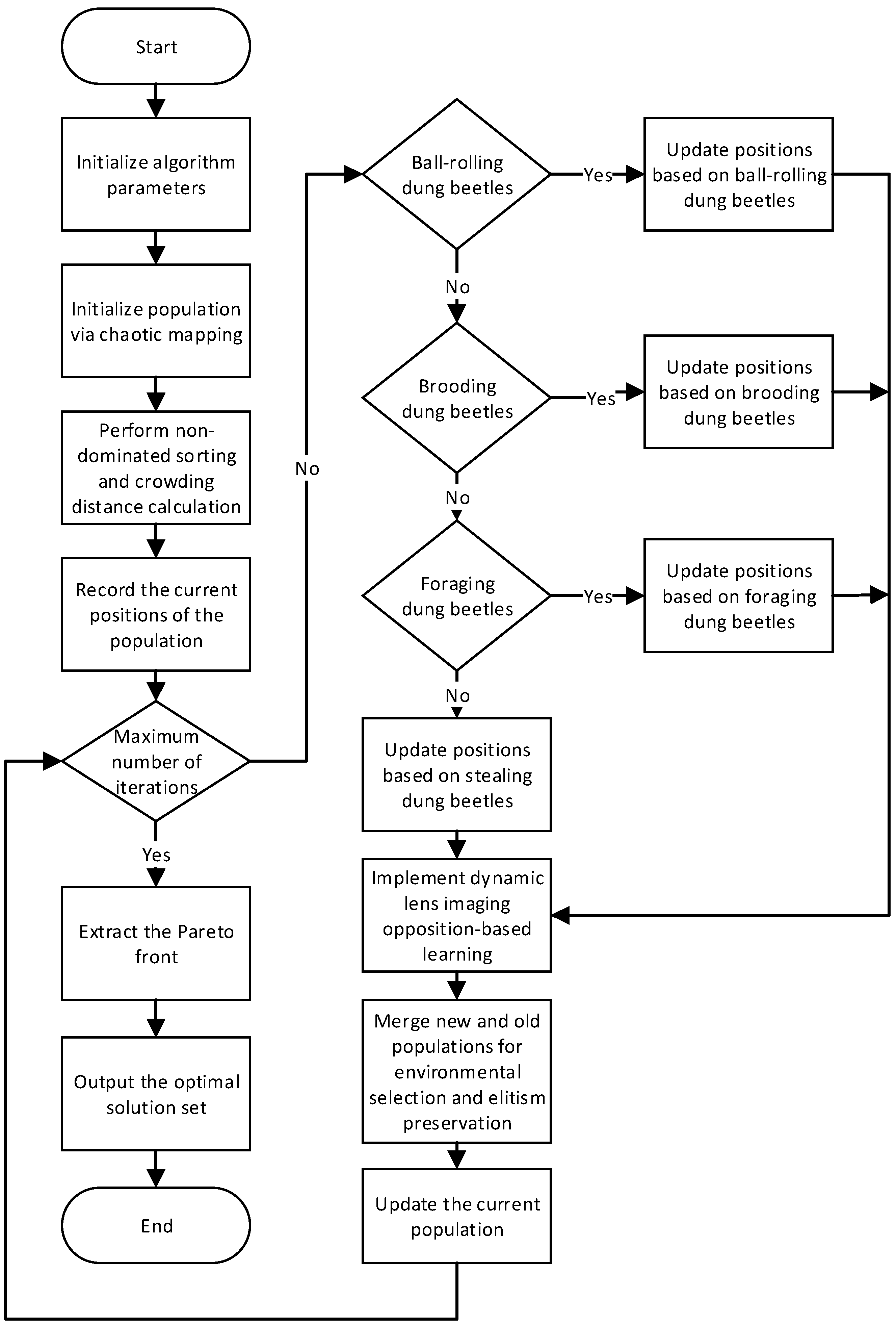
The flowchart of the MG optimization scheduling model based on MO-CLDBO is shown in Figure 1.
Figure 1 depicts the step-by-step workflow of the MO-CLDBO algorithm for microgrid economic-environmental dispatch. The algorithm first initializes parameters and generates an initial population using chaotic mapping. Individuals are evaluated via non-dominated sorting and crowding distance calculation before entering the main iteration loop. If the termination criterion is unmet, positions are updated by simulating four dung beetle behaviors. A dynamic lens imaging opposition-based learning strategy is then adaptively activated with a nonlinearly decaying probability, followed by population merging and elite-preserving environmental selection. The algorithm stops upon reaching the maximum iterations and outputs an evenly distributed Pareto optimal front for microgrid scheduling.

5. Simulation Results and Discussion

To validate the effectiveness of the proposed stochastic expected dispatch model for multi-objective economic-environmental microgrid dispatch and the superiority of the MO-CLDBO algorithm in solving high-dimensional complex optimization problems, comprehensive simulation tests are conducted on the MATLAB R2025a platform in this section.

5.1. Parameter Settings of the Microgrid System

This section presents a case study on a typical microgrid system. The dispatch horizon is 24 h with a 1-h time step. The system comprises three micro gas turbines (MTs), three diesel generators (DGs), a battery energy storage system (BESS), wind and solar power units. With continuous decision variables for each time slot, the established multi-objective economic-environmental dispatch model forms a high-dimensional nonlinear optimization problem with 168 variables (3 MTs, 3 DGs, 1 BESS, 24 hourly outputs for each unit). The parameters of the dispatchable distributed generators in the microgrid system are presented in Table 1, the pollutant treatment coefficients are shown in Table 2, the parameters of the energy storage system are listed in Table 3, and the time-of-use electricity prices are given in Table 4.
In the main comparison, all algorithms were configured with a population size of N = 50 and a maximum iteration count of T = 500 to ensure sufficient convergence. For the ablation study, all four variants shared identical configurations with N = 50 and T = 300 , as the objective was to compare the relative performance among algorithm variants rather than their absolute convergence behavior. Within each independent experiment, all compared algorithms adopted the same parameter settings and the same stopping criterion—strictly terminating upon reaching the maximum iteration count—to guarantee a fair comparison. Furthermore, all solvers employed a unified hybrid constraint-handling approach and a unified penalty function for power balance, ensuring the fairness of the benchmark results.

5.2. Optimal Scheduling of Microgrid Under Typical Wind-PV Output Scenarios

5.2.1. Wind-PV Scenario Generation Based on Gaussian Copula and Monte Carlo Sampling

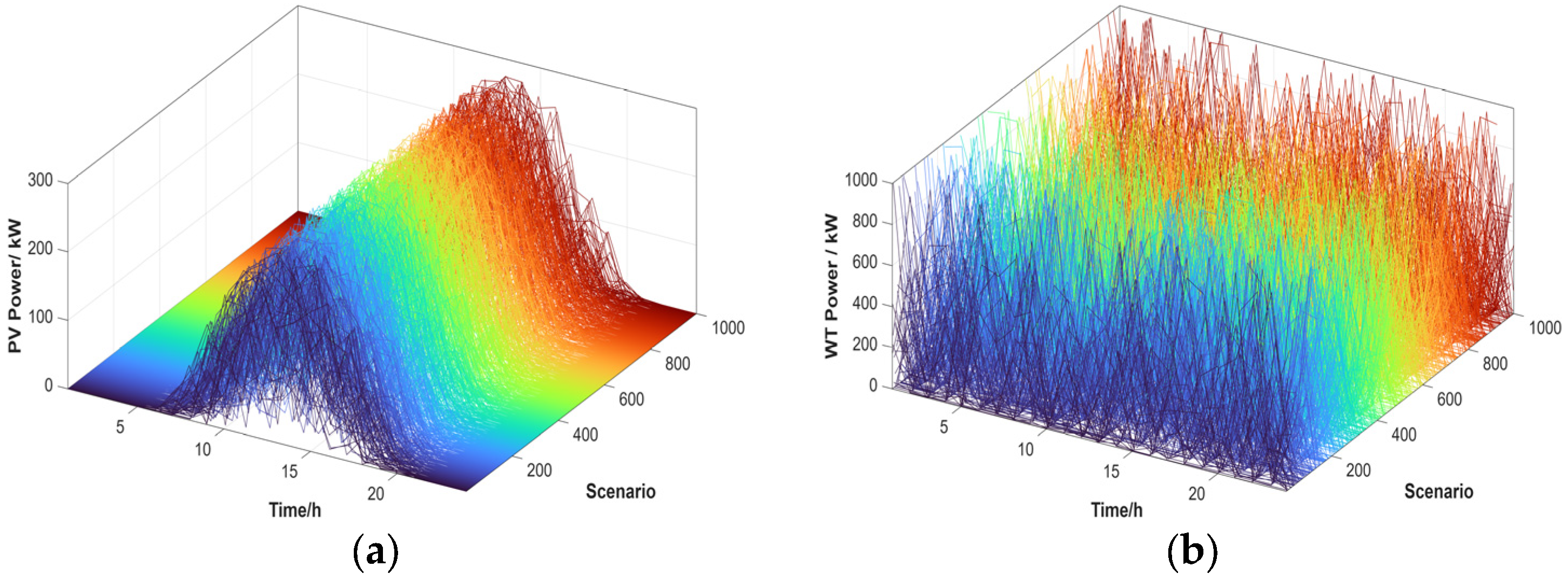
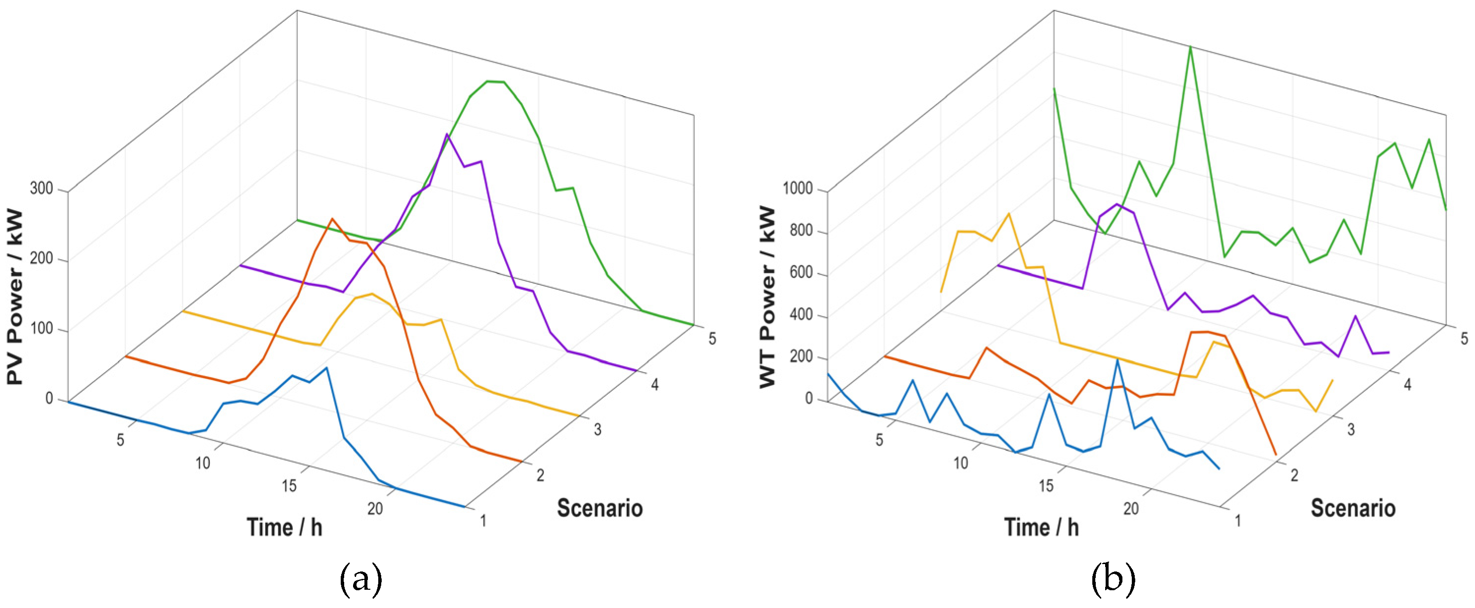
The actual outputs of wind power and photovoltaic arrays are not only subject to random disturbances from extreme weather conditions but also exhibit strong temporal autocorrelation over the 24-h day-ahead operation cycle. To faithfully reproduce this physical characteristic in the microgrid dispatch model, this paper abandons the traditional independent probability assumption and adopts a composite strategy of “Gaussian Copula function joint modeling + Monte Carlo sampling (MCS)” to generate the basic scenario set, as shown in Figure 2.
The generated scenarios conform to the diurnal variation rule of renewable energy output. PV power falls to zero at night and presents a typical parabolic distribution in daytime.
In terms of power magnitude and scenario range, the generated samples covered both normal operating states and extreme conditions, including a sharp PV drop due to sudden severe weather and high nighttime wind power output. Such diverse samples facilitate the robustness test of the multi-objective dispatch algorithm.
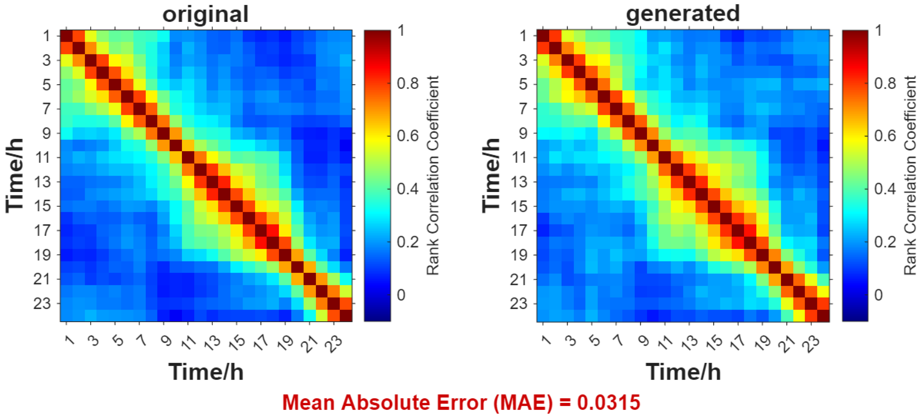
To further verify whether the generated scenarios preserve the temporal correlation of actual natural variations, the Spearman correlation matrix was adopted. Figure 3 presents the 24-h correlation heatmap between the original wind speed data and Copula-generated series.
The bilateral matrix topological features in Figure 3 indicate that both the generated scenarios and the original data exhibited a strong positive correlation coupling (highlighted in dark red) near the main diagonal. Moreover, the correlation decayed nonlinearly and smoothly as the time span increased, with the color gradually changing from dark red to blue, indicating a gradual weakening of the correlation. Quantitative calculation showed that the mean absolute error (MAE) between the two matrices was as low as 0.0315. This extremely small error quantitatively confirms that the proposed Copula framework accurately reconstructs the 24-h real spatiotemporal dependence structure, overcoming the issues of temporal fragmentation and physical distortion caused by traditional independent sampling. For example, it eliminated unrealistic phenomena such as strong wind at 9 a.m. but sudden zero wind speed at 10 a.m. in the generated samples.
Table 5 summarizes the goodness-of-fit results of the marginal distributions and the overall accuracy of the generated scenarios. For parametric marginal models, the one-sample Kolmogorov–Smirnov (K–S) test yielded an average p-value of 0.1896 for beta-fitted solar irradiance (daytime hours) and 0.1844 for the normal-fitted electric load (24 h), both above the 0.05 significance level, which supports the validity of the selected distribution forms. For wind speed, a rank-based nonparametric empirical cumulative distribution function was adopted for marginal transformation, and wind power output was further derived via the turbine power curve. This data-driven approach avoids parametric fitting bias by preserving the full statistical characteristics of raw data; the parametric one-sample K–S test is therefore not applicable (marked as N/A in Table 5).
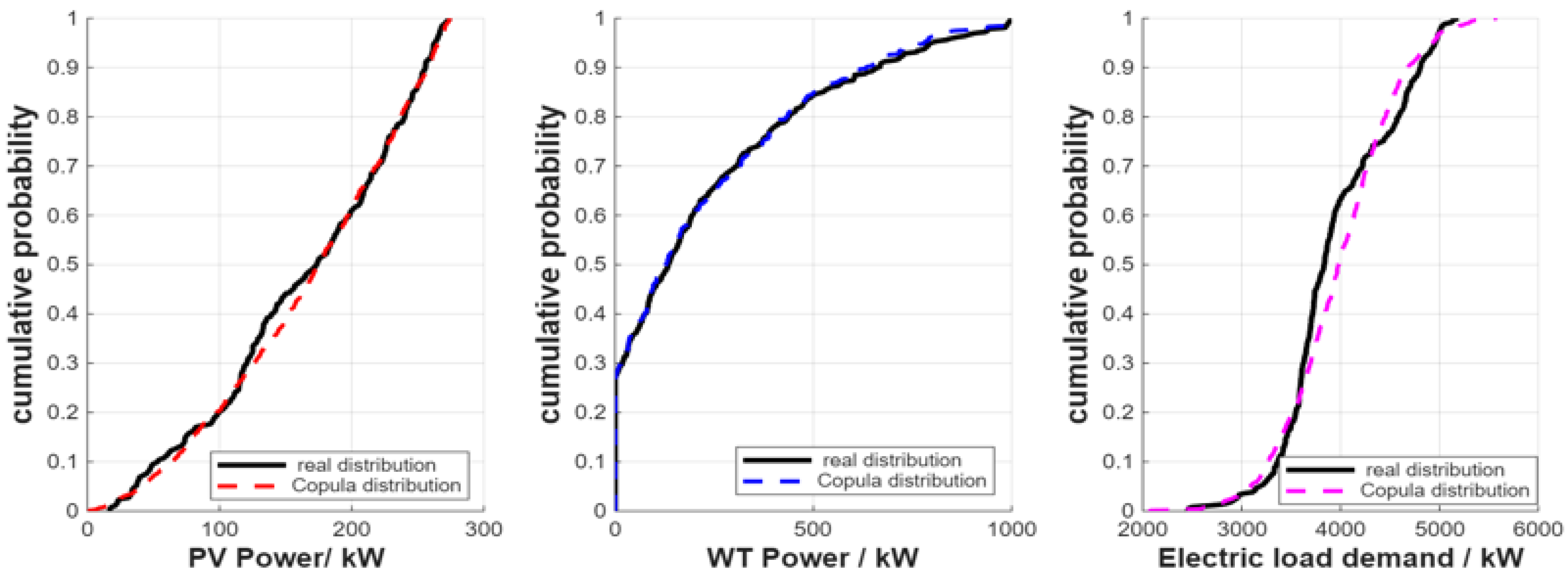
To further validate the overall fidelity of the generated scenarios, Figure 4 presents a comparison of the cumulative distribution functions (CDFs) between 1000 scenarios generated by the Gaussian Copula model and 8760-h full-year historical data, selected at typical peak hours (12:00 for photovoltaic output, 18:00 for wind turbine output and electrical load). The CDF curves of the generated scenarios aligned closely with those of the historical data, demonstrating that the proposed method can effectively reproduce the near-normal distribution characteristics of the electrical load, the nonlinear fluctuation of photovoltaic output, and the two-end clamping behavior of wind power output at zero and rated capacity. Over a 24-h horizon, the average errors of the mean and standard deviation for each variable were 2.00%/1.81% for photovoltaic output, 1.91%/2.14% for wind power output, and 0.65%/0.76% for electrical load, respectively.
The marginal goodness-of-fit tests, consistent visual CDF performance, and low quantitative moment errors together suggest the high-fidelity reproduction capability of the proposed model for probability distributions, which can provide reasonable uncertainty boundaries for subsequent microgrid optimal dispatch.

5.2.2. Scenario Reduction Based on Simultaneous Backward Reduction (SBR)

Although the large number of Copula-sampled scenarios can comprehensively cover the uncertainty boundaries, directly incorporating all of them into the multi-objective dispatch model with 168 decision variables would inevitably lead to the curse of dimensionality. Therefore, this paper introduces the simultaneous backward reduction (SBR) algorithm to reduce the initial scenario set. Moreover, it is worth emphasizing that in light of the multi-source heterogeneous characteristics of microgrids, this paper abandons the conventional paradigm of independently reducing wind and solar scenarios, which tends to break the spatial and physical correlations within the same meteorological day. Instead, it innovatively concatenates the time-series outputs of wind and solar power at each interval into a joint state vector. Based on this high-dimensional joint space, the SBR method sequentially eliminates redundant scenarios with the smallest probability-weighted distance and strictly transfers their occurrence probabilities to the nearest scenarios in the retained set.
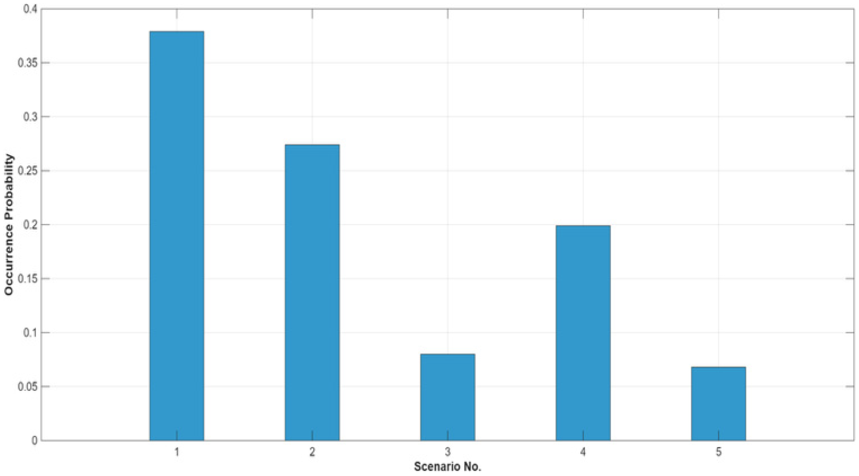
After SBR dimensionality reduction, the system successfully reduced 1000 initial joint scenarios to 5 highly representative typical joint scenarios with high fidelity. Due to the joint reduction mechanism, the photovoltaic and wind power outputs in any typical scenario set share the same occurrence probability, effectively preserving the “spatial synchrony” under the same meteorological conditions. Figure 5 shows the evolution curves of photovoltaic and wind power outputs under the five typical scenarios, respectively.
As shown in Figure 5, the five typical scenarios after reduction not only had distinct physical characteristics but also perfectly inherited the fluctuation envelopes of the initial scenario set. For example, the photovoltaic output accurately reflects the day-ahead radiation differences between “clear sky and intense sunlight” and “cloudy and rainy” conditions across different typical scenarios, while the wind power output reproduces the physical memory of high-frequency fluctuations at night and sustained long-duration outputs.
The discrete occurrence probability distribution of each typical scenario after simplification is illustrated in Figure 6 and Table 6.

5.2.3. Price-Based Demand Response (PBDR)

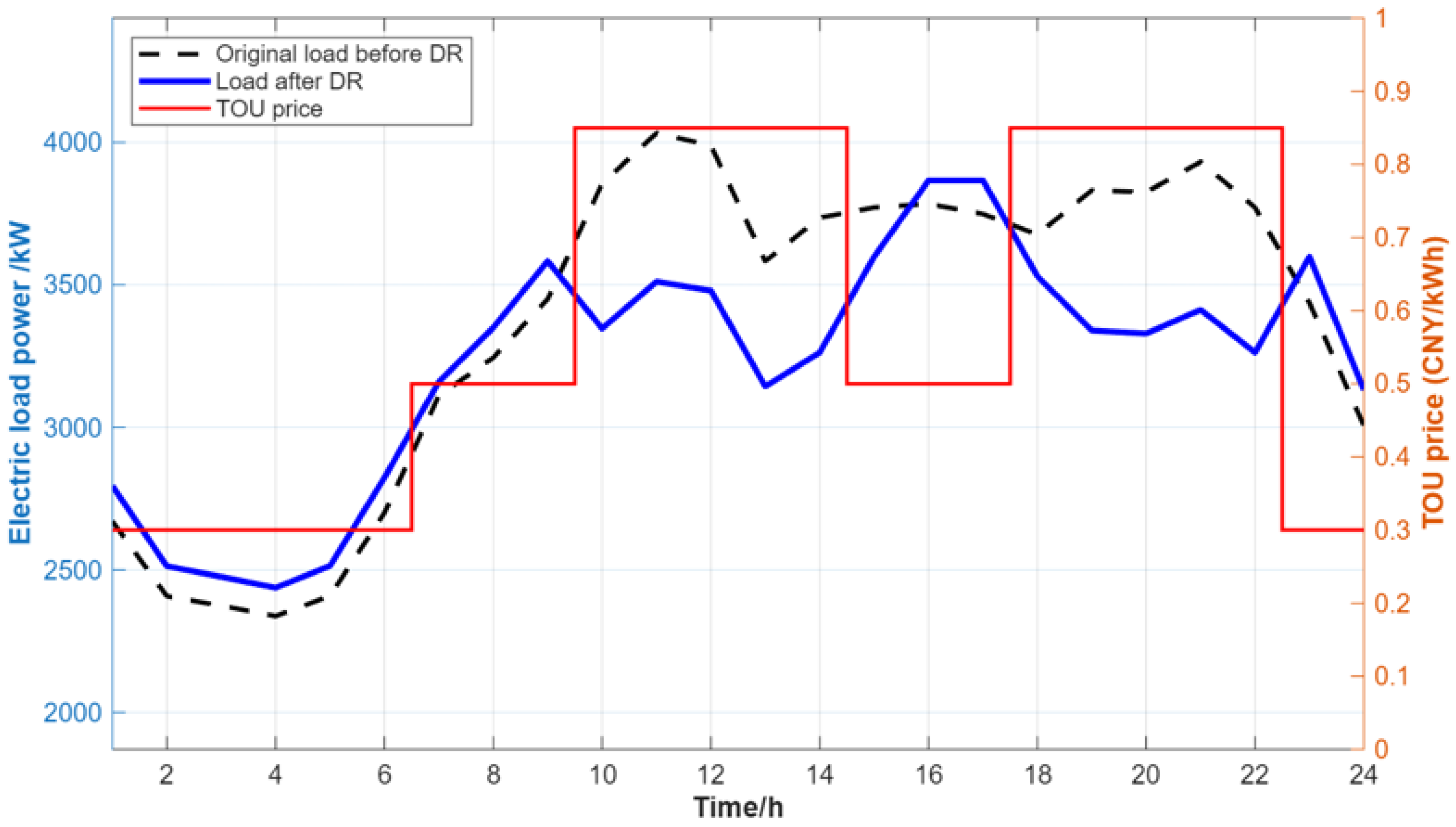
This paper introduces a price-based demand response (PBDR) model on the load side of the day-ahead dispatch. Driven by the time-of-use (TOU) tariff mechanism of the day-ahead main grid and the price elasticity matrix, the original rigid load of the microgrid achieves effective peak shaving and valley filling on the time axis. The comparison of the system total load evolution curves before and after the introduction of PBDR optimization is shown in Figure 7.
As can be seen from Figure 7, during the high time-of-use electricity price periods of 10:00–12:00 and 19:00–21:00, the system successfully shed a large amount of shiftable load. Most of the reduced peak load was shifted to the off-peak nighttime period from 01:00 to 08:00. Quantitative analysis shows that the PBDR mechanism reduced the peak load by 4.13% and increased the valley load by 4.26%, effectively flattening the load curve.

5.2.4. Ablation Study

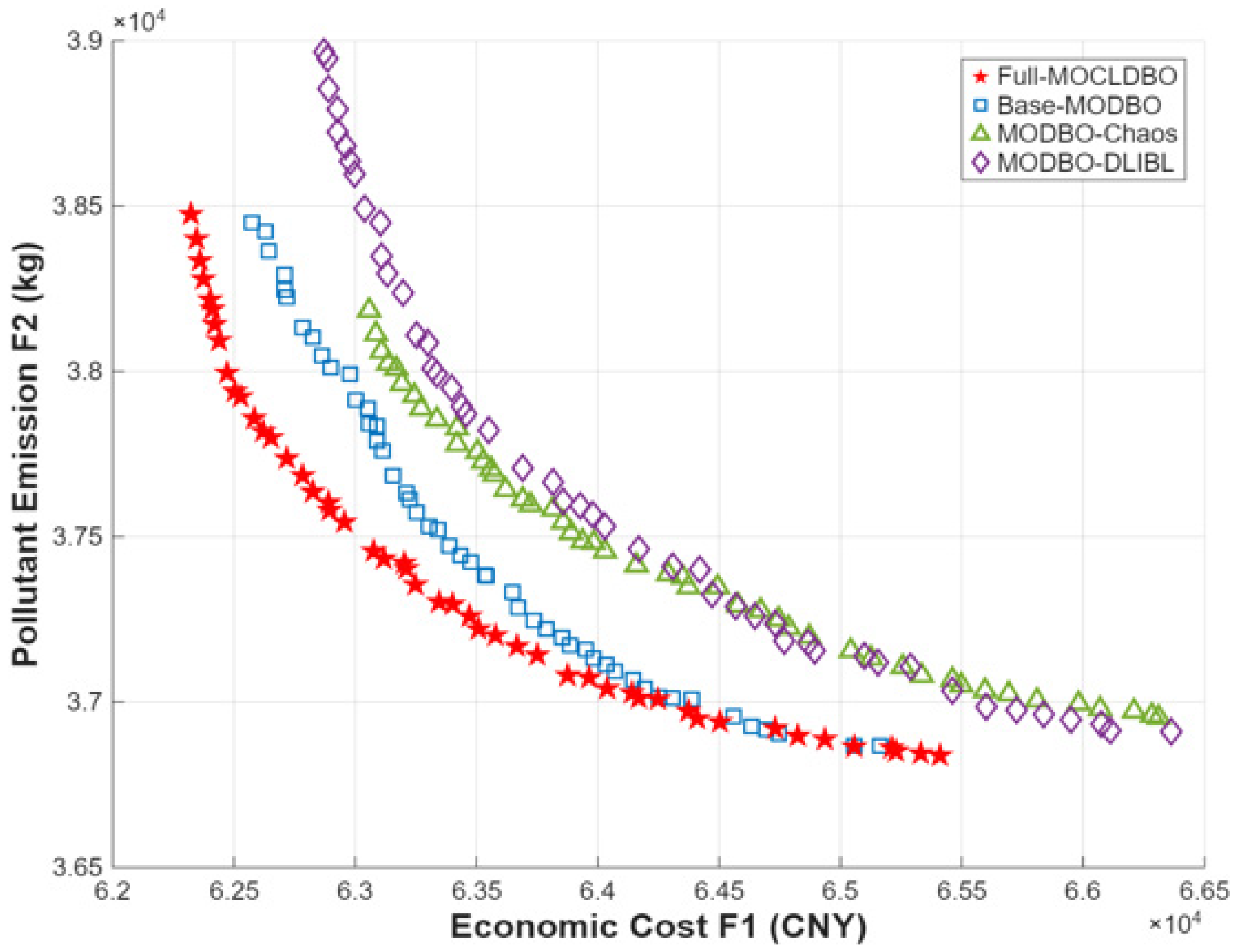
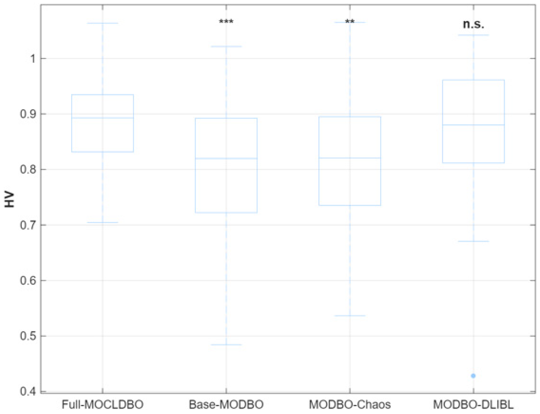
To verify the contribution of each improved module in the proposed MO-CLDBO, an ablation study involving four comparative schemes constructed based on the basic multi-objective dung beetle optimizer was conducted. All algorithms were run independently 50 times under the same parameter settings and scheduling constraints. The Pareto front comparison of different algorithmic variants in the multi-objective ablation study is shown in Figure 8, and each metric is listed in Table 7. Furthermore, the boxplot of the hypervolume (HV) indicator distributions for different algorithmic variants in the ablation study is illustrated in Figure 9.
As validated by the quantitative results in Table 7 and the statistical distributions in Figure 9, the hypervolume (HV) metrics showed a consistent upward trend from the baseline algorithm to the full MO-CLDBO framework (rising from 0.7987 to 0.8842), reflecting the positive contribution of each added improvement module to the overall algorithm performance. Visually, the representative Pareto front trajectories in Figure 8 confirm that the proposed Full-MOCLDBO achieved the leftmost bottom boundary among all variants, and performed geometric dominance over the baseline and single-improvement variants. Notably, although the MODBO-Chaos variant achieved the lowest average cost among all counterparts, its overall HV remained significantly inferior to that of the complete Full-MOCLDBO. This phenomenon demonstrates that while relying solely on chaotic initialization can aggressively accelerate early-stage convergence toward cost-optimal individuals, it fails to preserve population diversity along the emission dimension, ultimately triggering a structural deflation and fragmentation of the resulting Pareto front. With a Wilcoxon p-value of 0.801, the performance gap between Full-MOCLDBO and MODBO-DLIBL failed to reach the 0.05 significance level, verifying DLIBL as the core driver of performance enhancement. The introduction of Folded 2D-MCLSM chaotic initialization delivered a marginal improvement in average HV, making the full framework the top-performing variant. This marginal gain, despite statistical insignificance, still contributed positively to the robustness and uniform distribution of the Pareto front.
Additionally, it should be noted that the HV was computed using a normalized objective space with a reference point set slightly above the maximum observed values, following the standard HV definition. This ensures that the HV metric accurately reflects both the convergence and diversity of the obtained Pareto fronts.

5.2.5. Performance Comparison of Multi-Objective Optimization Algorithms

In this section, the performance of the proposed improved algorithm is compared with four mainstream advanced algorithms. Considering the inherent randomness of swarm intelligence algorithms, all algorithms were configured with the same population size N = 50 and maximum number of iterations T = 500 in the 168-dimensional decision space, and each algorithm was independently run 50 times to eliminate accidental errors.
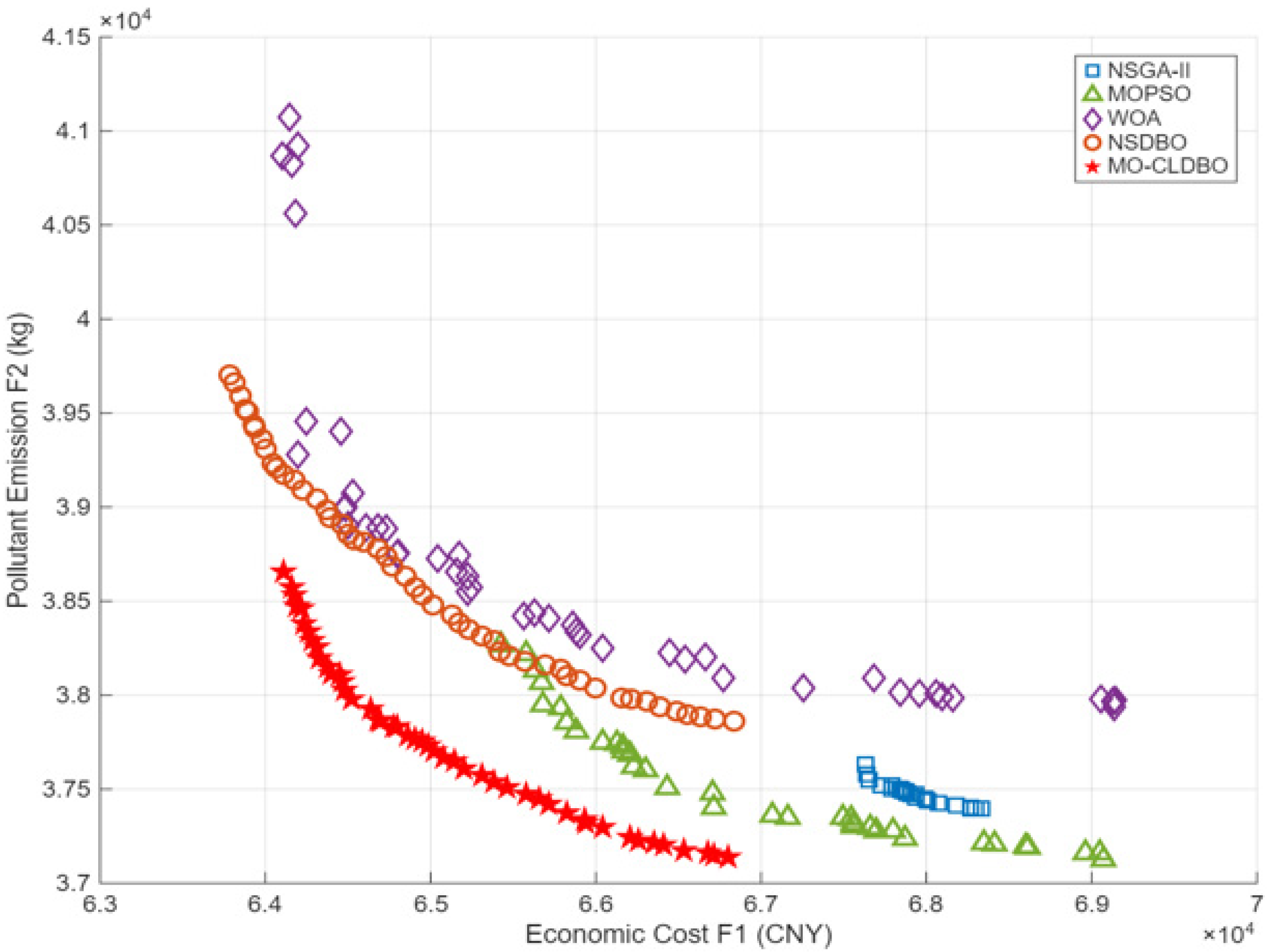
Figure 10 presents the Pareto front comparison of the five algorithms under the dual objectives of economic cost and environmental emission. It is evident that MO-CLDBO achieved a wider distribution of the front and a higher degree of approximation to the true frontier. Compared with the obvious discontinuities or clustering phenomena observed in the fronts of traditional algorithms such as NSGA-II, the front constructed by MO-CLDBO exhibited excellent continuity and smoothness, which directly demonstrates that the proposed chaotic mapping initialization and backward learning strategies effectively prevent the “front collapse” problem of the algorithm in the dispatch model.
Under the same experimental environment, each algorithm was tested with 50 independent runs, and the comprehensive performance statistical indicators are shown in Table 8 and Table 9. The results show that MO-CLDBO achieved the highest hypervolume (HV) value among all compared algorithms, which indicates that the proposed algorithm obtained the best overall Pareto-front quality and the most balanced cost–emission trade-off.
In terms of individual objective performance, MO-CLDBO obtained the lowest average comprehensive operating cost of 64,879 CNY with a standard deviation of 412, demonstrating stronger optimization stability and local optima avoidance capability than algorithms such as WOA and NSGA-II. It should be noted that NSGA-II and MOPSO yielded lower average emission values, but this came at the cost of higher operating costs. This indicates that these algorithms tend to converge to a different region of the objective space, which prioritizes emissions reduction at the expense of economic performance. In contrast, MO-CLDBO avoids the partial premature convergence trap and achieves a compromise solution with higher engineering application value by well coordinating the two conflicting objectives.
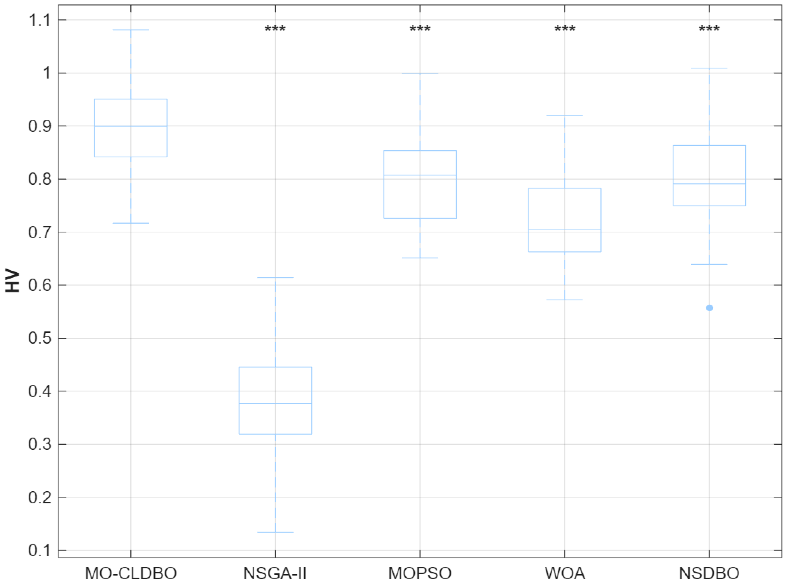
Second, in terms of the core metric for evaluating the overall quality of multi-objective Pareto fronts, i.e., the hypervolume (HV), MO-CLDBO achieved an average HV as high as 0.8992, far exceeding the other algorithms. Moreover, as shown in Figure 11, the boxplot of MO-CLDBO exhibited the highest overall position, the highest median value, and the narrowest interquartile range, indicating minimal dispersion across runs and the strongest robustness. This visual evidence is further corroborated by the quantitative results in Table 9, which presents the mean and standard deviation (±Std) of all metrics over 50 independent runs, along with the Wilcoxon rank-sum test results. Rather than relying on arbitrary single-run trajectory curves, this work quantifies the multi-objective convergence behavior through the statistical distribution of the hypervolume (HV) metric. Since the HV metric simultaneously reflects both convergence accuracy and Pareto front diversity, the superior mean HV (0.8992) and remarkably small standard deviation (±0.0778) of the proposed MO-CLDBO quantitatively demonstrate its stable and reliable convergence performance. In addition, the proposed algorithm also achieved favorable performance in terms of the spacing metric. Regarding computational efficiency, Table 9 presents the detailed statistical runtime results from 50 independent runs. The proposed MO-CLDBO achieved an average execution time of only 18.34 s, corresponding to a 59.4% reduction in runtime compared with NSGA-II (45.14 s) and a 46.1% reduction compared with WOA (34.04 s). More importantly, compared with the baseline NSDBO (17.37 s), the newly introduced operators incurred a negligible overhead of less than 1 s, corresponding to a mere 5.6% increment. This quantitatively demonstrates that the proposed algorithm achieves substantial multi-objective optimization performance gains at an extremely low additional computational cost.
Finally, the Wilcoxon rank-sum test shows that the p-values of all comparative algorithms versus MO-CLDBO were strictly below the significance level of 0.05, which statistically validates the effectiveness and superiority of the proposed improvement strategies.
To further quantify the magnitude of the observed differences, we calculated Cohen’s d effect sizes and 95% confidence intervals for HV comparisons, as shown in Table 10. The effect sizes were 8.542, 1.362, 2.046, and 0.576 for MO-CLDBO vs. NSGA-II, MOPSO, WOA, and NSDBO, respectively. The 95% confidence intervals did not cross zero for any comparison, confirming the statistical reliability of the improvements. These results indicate that MO-CLDBO provides very large to medium effects over the compared algorithms.
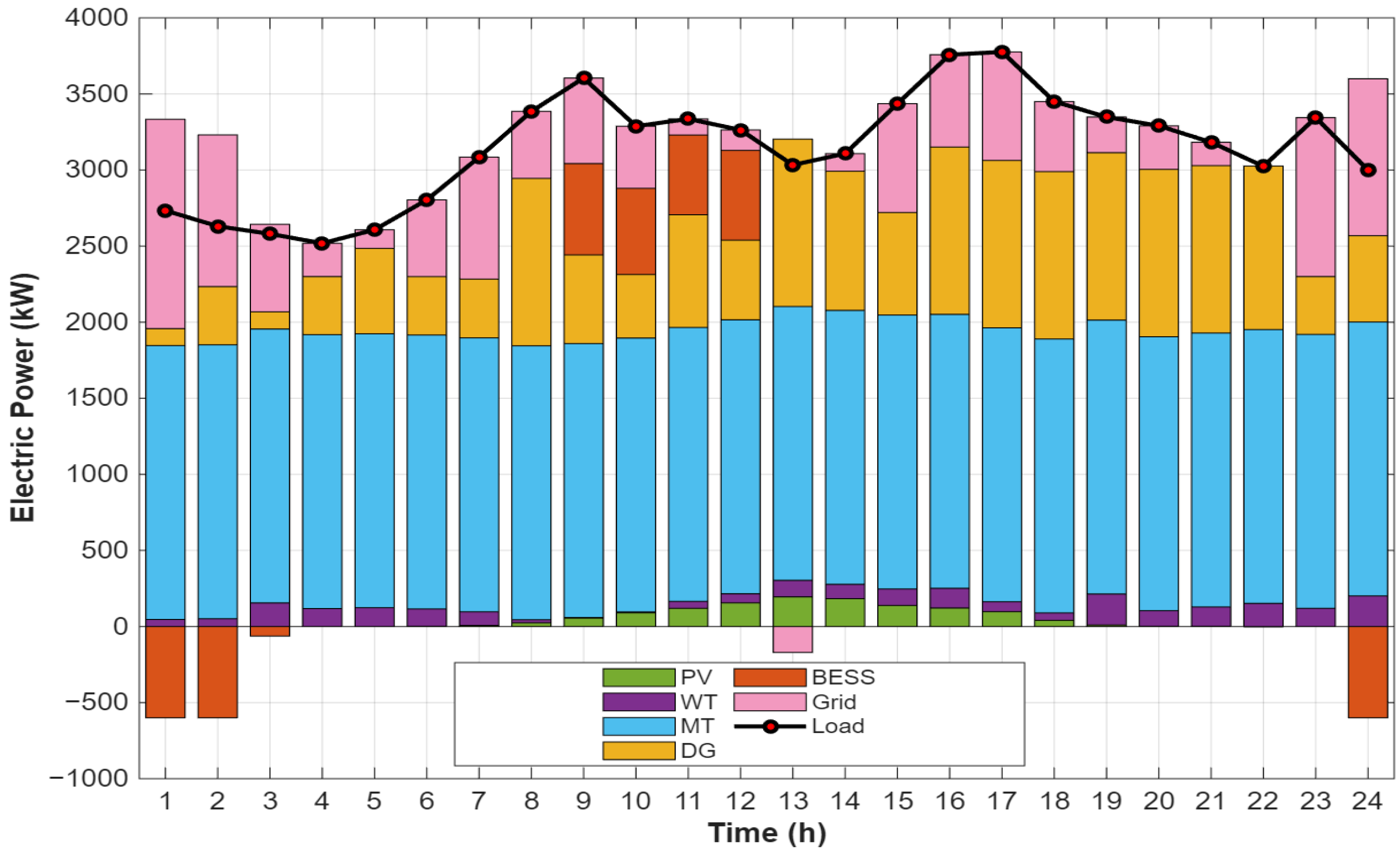
Figure 12 shows the power output configuration of the microgrid when considering demand response and wind–solar uncertainty.
As can be seen from Figure 12, at any time throughout the 24-h day, the sum of the positive power supply bars exactly equaled the sum of the absolute values of the net load curve and the negative absorption bars. This proves that after the complex high-dimensional non-convex multi-objective optimization, the algorithm always strictly satisfies the power balance equality constraint of the microgrid, and no physical violation of the solution occurs. The distribution of the PV and wind power bars in the figure shows that renewable energy outputs are prioritized by the system, which not only maximizes the utilization of renewable energy, but also greatly reduces the overall pollutant emissions of the system. The energy storage system exhibits significant activity. During the early morning hours when the load is low and wind power is abundant, the energy storage system performs charging; during the daytime peak hours and the evening peak, it discharges intensively to shave the peaks. This charging/discharging strategy not only alleviates the power supply pressure on the main grid and conventional units, but also achieves significant economic arbitrage by exploiting the peak–valley electricity price difference. Additionally, when the PV output drops sharply during the evening peak, the micro-turbines and diesel generators ramp up rapidly, supplemented by an appropriate amount of power purchased from the main grid, firmly covering the load deficit.
In summary, the dispatch scheme produced by the MO-CLDBO algorithm is a highly coordinated “source–grid–load–storage” strategy that deeply integrates renewable energy accommodation, temporal arbitrage of energy storage, and smooth power output of controllable units, fully demonstrating the algorithm’s outstanding engineering applicability in complex microgrid operation scenarios.

6. Conclusions

This paper addresses the day-ahead dispatch problem of microgrids with high-penetration distributed generation and complex flexible loads by constructing a multi-objective environmental economic dispatch model that accounts for wind–solar uncertainty and price-based demand response. An improved multi-objective dung beetle optimization algorithm integrating hyperchaotic mapping and dynamic lens imaging backward learning was proposed. Through simulations and rigorous statistical tests, the following core conclusions can be drawn:
(1) Uncertainty modeling and demand response mechanism: The multivariate joint probability model based on the Gaussian Copula function effectively captures the physical coupling characteristics of wind speed and solar irradiance in temporal evolution. The introduction of the PBDR mechanism achieves deep peak shaving and valley filling of the load curve, significantly enhancing the physical feasibility and security of the day-ahead microgrid dispatch scheme.
(2) Algorithmic optimization performance: The combination of Folded 2D-MCLSM chaotic initialization and the DLIBL backward learning strategy effectively alleviates the premature convergence defect of the original DBO algorithm when dealing with high-dimensional non-convex constraints. MO-CLDBO effectively mitigates the Pareto front collapse tendency that easily occurs in the late stage of traditional multi-objective evolution with non-dominated sorting, and maintains favorable population diversity and uniform distribution capability in complex multimodal solution spaces.
(3) Multi-objective comprehensive benefits and statistical verification: Statistical results from 50 independent runs show that MO-CLDBO achieved the lowest average comprehensive operating cost (64,879 CNY) and the highest average hypervolume (HV, 0.8992) among compared classical algorithms such as NSGA-II and MOPSO. The highest HV value indicates that the proposed algorithm delivered the best overall Pareto-front quality and the most balanced cost–emission trade-off. The Wilcoxon rank-sum test results (all p-values far below 0.05) rigorously verify the statistically significant improvement of the proposed algorithm in overall multi-objective optimization performance. The proposed scheduling framework can provide microgrid decision-makers with well-distributed optimal compromise solutions, realizing a coordinated balance between economic benefits and low-carbon environmental protection.
Future work will consider extending this dispatch framework to multi-microgrid cluster interconnection scenarios and explore the introduction of deep reinforcement learning techniques to cope with real-time dynamic fluctuations of sources and loads on shorter time scales.


Author Contributions

Conceptualization, J.L.; methodology, J.L. and L.K.; software, J.L.; validation, J.L. and L.K.; data curation, F.C.; writing—original draft preparation, J.L.; writing—review and editing, L.K. and H.L. All authors have read and agreed to the published version of the manuscript.

Funding

This work was supported by the Project of the Educational Department of Liaoning Province (LJ242511632005, LJ212411632068).

Data Availability Statement

The data presented in this study are available on request from the corresponding author. The data are not publicly available due to the data in the text relating to the privacy of electricity use in the regional distribution grid.

Conflicts of Interest

The authors declare no conflicts of interest.

References

  1. Wang, H.; Xu, Y.; Yi, Z.; Xu, J.; Xie, Y.; Li, Z. A review on economic dispatch of power system considering atmospheric pollutant emissions. Energies 2024, 17, 1878. [Google Scholar] [CrossRef]
  2. Hirsch, A.; Parag, Y.; Guerrero, J. Microgrids: A review of technologies, key drivers, and outstanding issues. Renew. Sustain. Energy Rev. 2018, 90, 402–411. [Google Scholar] [CrossRef]
  3. Xiang, Y.; Li, L.; Li, R.; Zhang, X.; Gu, C.; Zeng, P.; Pu, T.; Liu, J. Design flexible renewable energy penetrated power system to address long-run and short-run interactive inference. Innov. Energy 2024, 1, 100042. [Google Scholar]
  4. National Energy Administration of China. National Energy Administration Releases 2025 National Power Statistics [EB/OL]; National Energy Administration: Beijing, China, 2026.
  5. Shu, Y. Research and application of UHV power transmission in China. High Volt. 2018, 3, 3–13. [Google Scholar] [CrossRef]
  6. Mao, C.; Wang, R.; Zhou, Y.; Yuan, Y.; Zhong, J.; Huang, K. Research on Typical DC Fault Characteristics of±1100 kV Converter Station. In Proceedings of the 2021 6th International Conference on Power and Renewable Energy (ICPRE); IEEE: New York, NY, USA, 2021; pp. 250–255. [Google Scholar]
  7. Olivares, D.E.; Mehrizi-Sani, A.; Etemadi, A.H.; Canizares, C.A.; Iravani, R.; Kazerani, M.; Hajimiragha, A.H.; Gomis-Bellmunt, O.; Saeedifard, M.; Palma-Behnke, R.; et al. Trends in microgrid control. IEEE Trans. Smart Grid 2014, 5, 1905–1919. [Google Scholar] [CrossRef]
  8. Blinov, I.V.; Parus, Y.e.V.; Artemchuk, V.O. Prosumer Operation Planning Model in the Retail Electricity Market. Tech. Electrodyn. 2026, 1, 50–61. [Google Scholar] [CrossRef]
  9. Abido, M.A. Environmental/economic power dispatch using multiobjective evolutionary algorithms. IEEE Trans. Power Syst. 2003, 18, 1529–1537. [Google Scholar] [CrossRef]
  10. Al-kubragyi, S.; Abdulla, S.; Ali, I.I.; Alwazni, H.; Mohsen, S. Solving the Multi-objective Economic-Emission Load Dispatch Optimization Problem Using Hybrid GWO-PSO Algorithm. Int. J. Intell. Eng. Syst. 2024, 17. [Google Scholar] [CrossRef]
  11. Zhu, X.; Ruan, G.; Geng, H.; Liu, H.; Bai, M.; Peng, C. Multi-objective sizing optimization method of microgrid considering cost and carbon emissions. IEEE Trans. Ind. Appl. 2024, 60, 5565–5576. [Google Scholar] [CrossRef]
  12. Zakaria, A.; Ismail, F.B.; Lipu, M.H.; Hannan, M. Uncertainty models for stochastic optimization in renewable energy applications. Renew. Energy 2020, 145, 1543–1571. [Google Scholar] [CrossRef]
  13. Mishra, S.; Shaik, A.G. Solving bi-objective economic-emission load dispatch of diesel-wind-solar microgrid using African vulture optimization algorithm. Heliyon 2024, 10, e24993. [Google Scholar] [PubMed]
  14. Zheng, K.; Sun, Z.; Song, Y.; Zhang, C.; Zhang, C.; Chang, F.; Yang, D.; Fu, X. Stochastic scenario generation methods for uncertainty in wind and photovoltaic power outputs: A comprehensive review. Energies 2025, 18, 503. [Google Scholar] [CrossRef]
  15. Sklar, M. Fonctions de répartition à n dimensions et leurs marges. Ann. De L’ISUP 1959, 8, 229–231. [Google Scholar]
  16. Zhao, B.; Jiang, M.; Wang, X.; Wang, R.; Xiong, J.; Yang, N.; Li, Z. A Typical Scenario Generation Method Based on KDE-Copula for PV Hosting Capacity Analysis in Distribution Networks. Processes 2026, 14, 617. [Google Scholar] [CrossRef]
  17. Tan, J.; Zhang, J.; Liu, H.; Lan, B. A high dimensional uncertain scenario generating method for wind power and photovoltaic considering spatiotemporal correlation. Energy 2025, 340, 139224. [Google Scholar] [CrossRef]
  18. Shahryari, E.; Shayeghi, H.; Mohammadi-Ivatloo, B.; Moradzadeh, M. A copula-based method to consider uncertainties for multi-objective energy management of microgrid in presence of demand response. Energy 2019, 175, 879–890. [Google Scholar]
  19. Siano, P. Demand response and smart grids—A survey. Renew. Sustain. Energy Rev. 2014, 30, 461–478. [Google Scholar] [CrossRef]
  20. Li, D.; Jayaweera, S.K. Uncertainty modeling and price-based demand response scheme design in smart grid. IEEE Syst. J. 2014, 11, 1743–1754. [Google Scholar] [CrossRef]
  21. Wang, C.; Li, X. Optimization scheduling of microgrid comprehensive demand response load considering user satisfaction. Sci. Rep. 2024, 14, 16034. [Google Scholar] [CrossRef] [PubMed]
  22. Ma, Y.; Wang, P.; Hou, D.; Yu, Y.; Li, S.; Gao, T. Optimization Model of Time-of-Use Electricity Pricing Considering Dynamical Time Delay of Demand-Side Response. Energies 2025, 18, 2637. [Google Scholar]
  23. Tostado-Véliz, M.; Kamel, S.; Hasanien, H.M.; Turky, R.A.; Jurado, F. Uncertainty-aware day-ahead scheduling of microgrids considering response fatigue: An IGDT approach. Appl. Energy 2022, 310, 118611. [Google Scholar]
  24. Escamilla, J.E.A.; Zhou, L.; Zhu, X.; Wang, H. Towards Affordable Energy: A Gymnasium Environment for Electric Utility Demand-Response Programs. arXiv 2026, arXiv:2605.12462. [Google Scholar]
  25. Dewangan, C.L.; Singh, S.; Chakrabarti, S.; Singh, K. Peak-to-average ratio incentive scheme to tackle the peak-rebound challenge in TOU pricing. Electr. Power Syst. Res. 2022, 210, 108048. [Google Scholar]
  26. Alghamdi, H.; Hua, L.-G.; Hafeez, G.; Murawwat, S.; Bouazzi, I.; Alghamdi, B. Optimal adaptive heuristic algorithm based energy optimization with flexible loads using demand response in smart grid. PLoS ONE 2024, 19, e0307228. [Google Scholar] [CrossRef] [PubMed]
  27. Nassef, A.M.; Abdelkareem, M.A.; Maghrabie, H.M.; Baroutaji, A. Review of metaheuristic optimization algorithms for power systems problems. Sustainability 2023, 15, 9434. [Google Scholar] [CrossRef]
  28. Deb, K.; Pratap, A.; Agarwal, S.; Meyarivan, T. A fast and elitist multiobjective genetic algorithm: NSGA-II. IEEE Trans. Evol. Comput. 2002, 6, 182–197. [Google Scholar] [CrossRef]
  29. Coello, C.A.C.; Pulido, G.T.; Lechuga, M.S. Handling multiple objectives with particle swarm optimization. IEEE Trans. Evol. Comput. 2004, 8, 256–279. [Google Scholar] [CrossRef]
  30. Xue, J.; Shen, B. Dung beetle optimizer: A new meta-heuristic algorithm for global optimization. J. Supercomput. 2023, 79, 7305–7336. [Google Scholar]
  31. Palensky, P.; Dietrich, D. Demand side management: Demand response, intelligent energy systems, and smart loads. IEEE Trans. Ind. Inform. 2011, 7, 381–388. [Google Scholar] [CrossRef]
  32. Zhai, C.; Cao, Z.; Wang, Y.; Abdou-Tankari, M.; Yu, J.; Lei, Z. A reverse incentive-based demand response strategy for shared energy storage in industrial microgrids: Optimization, scheduling, and investment analysis. Energy 2025, 330, 136882. [Google Scholar] [CrossRef]
  33. Wang, R.; Ma, Y.; Zhao, X.; Tang, C.; Zhu, H.; Lu, S.; Sun, Y. A Grid-Friendly Aggregation Control Method for Split Air Conditioning Clusters Using Temperature-Gradient Strategy to Achieve Peak Shaving with Improved Comfort and Reduced Rebound. J. Build. Eng. 2026, 128, 116545. [Google Scholar]
  34. Zakariazadeh, A.; Jadid, S.; Siano, P. Smart microgrid energy and reserve scheduling with demand response using stochastic optimization. Int. J. Electr. Power Energy Syst. 2014, 63, 523–533. [Google Scholar] [CrossRef]
  35. Hassan, Z.M.; El-Saadawi, M.M.; Hatata, A.Y.; Sanjeevikumar, P.; Sedhom, B.E. Leveraging modified golden jackal optimization for enhanced demand-side management in microgrids with different tariffs. Energy Rep. 2025, 13, 3672–3685. [Google Scholar] [CrossRef]
Figure 1. Flowchart of MO-CLDBO.
Energies 19 03206 g001
Figure 2. PV and WT output curve of simulated scenario. (a) PV output; (b) WT output.
Energies 19 03206 g002
Figure 3. Comparison of 24-h temporal rank correlation coefficient matrices between the original historical wind speed and Copula-generated samples.
Energies 19 03206 g003
Figure 4. Empirical CDF comparison between full-year historical profiles and generated scenarios at representative peak hours.
Energies 19 03206 g004
Figure 5. Reduced photovoltaic power scenarios (a) and reduced wind power scenarios (b).
Energies 19 03206 g005
Figure 6. Probability of occurrence of typical scenarios.
Energies 19 03206 g006
Figure 7. Comparison of load curves before and after price-based demand response.
Energies 19 03206 g007
Figure 8. Pareto front comparison of different algorithmic variants in the multi-objective ablation study.
Energies 19 03206 g008
Figure 9. Comparison of hypervolume (HV) metrics for different algorithmic variants in the ablation experiment. *** denotes an extremely strong statistical dominance with a p -value less than 0.001 ( p < 0.001 ), ** represents a highly significant difference ( p < 0.01 ), n.s. (not significant) implies that the performance disparity is not statistically meaningful ( p 0.05 ).
Energies 19 03206 g009
Figure 10. Comparison of Pareto fronts for multi-unit microgrid.
Energies 19 03206 g010
Figure 11. Comparison of HV distribution of various algorithms after 50 independent runs. *** denotes an extremely strong statistical dominance with a p -value less than 0.001 ( p < 0.001 ).
Energies 19 03206 g011
Figure 12. MG output at the lowest total cost considering DR and the uncertainty of wind and solar power.
Energies 19 03206 g012
Table 1. Distributed generation parameters.
Equipment TypeUnit No.Power Limit/kWMaximum Ramp Rate/(kW/h)Operation & Maintenance Cost/(CNY/kWh)
MTMT 1[50, 500]2000.020
MT 2[50, 500]2000.020
MT 3[80, 800]3000.020
DGDG 1[30, 300]1500.025
DG 2[30, 300]1500.025
DG 3[50, 500]2500.025
WTWT 1[0, 250]00.008
PVPV 1[0, 200]00.005
Table 2. Pollutant emission coefficients.
Types of Pollutant GasesPollutant Emission Factor/(g/kWh)
MTDG
CO2450650
NOX1.02.0
Table 3. Parameter information of battery.
Parameter NameParameter
Max. Capacity/kWh3000
Max. Charge–Discharge Power/kW600
Min. Capacity/kWh300
Base Capacity/kWh1500
O&M Cost/[CNY/(kWh)]0.01
Charge–Discharge Rate0.95
Table 4. Time-of-use electricity price.
Time PeriodOff-PeakMid-PeakOn-Peak
00:00–06:5907:00–10:5911:00–13:59
22:00–23:5914:00–17:5918:00–21:59
Purchase Price/[CNY/(kWh)]0.30.71.2
Selling Price/[CNY/(kWh)]0.240.560.96
Table 5. Statistical goodness-of-fit and moment error verification.
Variable TypeOne-Sample K–S Test (Average p-Value)Mean ErrorStd Error
WTN/A1.91%2.14%
PV0.18962.00%1.81%
Load0.18440.65%0.76%
Table 6. Occurrence probability of typical joint scenarios.
Typical Scenario NumberProbability of Wind Power ScenariosProbability of PV Scenarios
10.3790.379
20.2740.274
30.080.08
40.1990.199
50.0680.068
Table 7. Quantitative ablation comparison.
AlgorithmAvg Cost (CNY)Avg HVAvg SpacingWilcoxon (p)
Full-MOCLDBO63,5430.88420.0118
Base-MODBO63,6100.79870.00968.59 × 10−4
MODBO-Chaos63,4900.81680.01042.80 × 10−3
MODBO-DLIBL63,5980.87030.01158.01 × 10−1
Table 8. Algorithm results.
AlgorithmMean Final ValueStandard Deviation of Final ValueMean Emission ValueStandard Deviation of Emission Value
MO-CLDBO64,87941238,146210
NSGA-II68,29348537,472103
MOPSO66,77167137,373214
WOA65,55484238,408337
NSDBO65,01038338,290167
Table 9. Algorithm metrics.
AlgorithmHV (Mean ± Std)Mean SpacingAvg Time (s)Wilcoxon Rank-Sum Test
MO-CLDBO0.8992 ± 0.07780.008418.34 s-
NSGA-II0.3820 ± 0.09460.004245.14 s7.07 × 10−18
MOPSO0.7992 ± 0.08260.016816.84 s8.65 × 10−8
WOA0.7183 ± 0.08230.022134.04 s2.65 × 10−14
NSDBO0.7943 ± 0.09170.007117.37 s1.09 × 10−7
Table 10. Effect sizes (Cohen’s d) and 95% confidence intervals for HV comparisons between MO-CLDBO and other algorithms.
ComparisonCohen’s d95% CI
MO-CLDBO vs. NSGA-II8.542[0.772, 0.825]
MO-CLDBO vs. WOA2.046[0.177, 0.233]
MO-CLDBO vs. MOPSO1.362[0.117, 0.179]
MO-CLDBO vs. NSDBO0.576[0.042, 0.125]
Disclaimer/Publisher’s Note: The statements, opinions and data contained in all publications are solely those of the individual author(s) and contributor(s) and not of MDPI and/or the editor(s). MDPI and/or the editor(s) disclaim responsibility for any injury to people or property resulting from any ideas, methods, instructions or products referred to in the content.