


Abstract
The classical Fortescue symmetrical-component transform remains fully invertible as a similarity transform when the complete sequence-domain matrix is retained. In practice, however, untransposed three-phase overhead lines are often summarized by the diagonal sequence quantities and , while the asymmetry appears through coupled off-diagonal terms that are less convenient for compact parameterization and measurement-based interpretation. This paper presents an Extended Sequence Transform that reorganizes the six independent entries of the phase-domain impedance matrix into six structured parameters by means of a lossless, invertible linear mapping. The first two parameters are identical to the classical zero- and positive-sequence impedances, which preserves backward compatibility. The remaining four parameters isolate asymmetry information in a form from which all entries of the classical sequence matrix can be recovered exactly, and from which the full phase-domain matrix is reconstructed to machine precision. The proposed representation does not diagonalize an untransposed line; rather, it provides a compact and explicit six-scalar parameterization that separates the classical sequence pair from four asymmetry descriptors. Numerical validation on a 50 km untransposed overhead line confirms exact round-trip reconstruction and exact agreement of the unbalance factors obtained from the classical and extended representations. A stochastic perturbation study further shows that round-trip reconstruction remains at numerical precision and that, within the tested perturbation grid, the factor is more sensitive than . Line-constant calculations performed in OpenDSS for two typical 400 kV tower geometries link the four asymmetry parameters to specific geometric features, a worked offline measurement example recovers them from simulated three-phase terminal tests, and a distributed-model study confirms that the lumped-parameter description of the asymmetry remains accurate to within about 0.6% up to 150 km.
1. Introduction
The Fortescue symmetrical-component transform [1] is the standard tool for power-system analysis. When applied to a three-phase overhead line, it diagonalises the impedance matrix of a perfectly transposed line into independent zero-sequence and positive-sequence networks. In practice, however, most high-voltage transmission lines are either untransposed or only partially transposed, resulting in a phase-domain impedance matrix with six distinct complex entries rather than two [2,3].
When the Fortescue transform is applied to the phase-domain impedance matrix of an untransposed three-phase line, non-zero off-diagonal terms appear in the sequence matrix, coupling the zero-, positive-, and negative-sequence networks and inducing voltage unbalance even under balanced loading.
The inductive unbalance factors [4] provide a standard approach to quantifying this coupling through two dimensionless percentages normalised against the zero- and positive-sequence impedances respectively, and serve effectively as asymmetry metrics for line characterisation. In common engineering use, however, the classical representation is often reduced to the two diagonal quantities and . That reduced description is not sufficient for an untransposed line, because the off-diagonal sequence couplings carry essential asymmetry information. If the complete matrix is retained, the Fortescue transform remains lossless and the original can be recovered exactly. The practical difficulty is therefore not mathematical invertibility, but rather that the full sequence matrix mixes asymmetry effects across several coupled terms and does not offer a compact six-scalar parameterization aligned with the familiar pair . Applications that require knowledge of the complete matrix, such as parameter identification from terminal voltage and current measurements on untransposed lines, therefore need a representation that retains the full information while exposing the asymmetry structure more explicitly [5,6].
The problem is further compounded when the line is supplied from an unbalanced source. When both the supply voltage and the line geometry are asymmetric, the measured sequence voltages and currents at the terminals reflect a combination of source asymmetry and line asymmetry that cannot be separated by inspection of terminal quantities alone. The line characteristics must therefore be described by a representation that is independent of the terminal voltages and currents and that admits lossless reconstruction of the full phase-domain impedance matrix.
Several alternative transformation frameworks have been proposed to address the limitations of symmetrical components for untransposed and asymmetric lines. Phase-domain methods replace sequence decomposition with direct phase variables so that a single circuit topology represents common shunt faults while explicitly modelling mutual coupling between phases [7]. The Clarke transform and related single-real transformation matrices offer a compact real-valued modal basis suitable for time-domain overvoltage studies and non-transposed line analysis [8,9]. The Karrenbauer transform and its corrected variants are derived specifically to restore modal decoupling for untransposed configurations where standard sequence transforms are inadequate [10]. Modal optimisation methods recast the eigenvalue problem as a constrained optimisation to obtain smooth, continuous transformation matrices across frequency, avoiding the eigenvector discontinuities of direct eigendecomposition [11,12].
These approaches pursue a different objective from the one considered here. Modal methods seek propagation-mode decoupling for simulation and frequency-dependent line modeling [11,12,13,14], whereas the present work seeks a compact parameterization of the full phase-domain impedance matrix that remains anchored to the classical sequence quantities and . The proposed transform therefore should not be viewed as a replacement for modal decomposition. Its role is to provide a structured six-parameter representation of the same reciprocal line matrix, with exact forward and inverse mappings and with asymmetry collected into four dedicated parameters.
This paper presents the Extended Sequence Transform, a lossless invertible six-by-six linear mapping from the six independent entries of the phase-domain impedance matrix to six extended sequence parameters. The key novelty is not the invertibility of the full Fortescue similarity transform itself, but the introduction of a structured six-parameter representation in which the classical pair is retained explicitly and the remaining four parameters capture the line asymmetry. This reparameterization preserves all six independent entries of the reciprocal phase-domain matrix and reconstructs them exactly. A further property is that two of the four new asymmetry parameters, denoted as the difference parameters and defined precisely in Section 4, are formed as differences of self- and mutual-impedance components at the same Fortescue wavenumber. This structure is potentially attractive in parameter-identification settings because it separates the mean sequence content from asymmetry content, as discussed in Section 6. To be precise about the scope of the contribution, the transform is an information-preserving change of basis on the six independent entries of the phase-domain matrix; it does not reduce the information dimension and it is not a new physical decomposition. It is also distinct in purpose from the Fortescue, Clarke, and Karrenbauer transforms, which act on the phase voltages and currents to pursue propagation-mode decoupling, whereas the proposed map acts on the entries of the impedance matrix itself. Invertibility is therefore a prerequisite rather than the result; the practical value, demonstrated in the revised manuscript, lies in relating the four asymmetry parameters to tower geometry (Section 6) and in recovering them from three-phase terminal measurements (Section 7).
All entries of the classical Fortescue sequence matrix are exactly expressible in terms of the extended parameters, and the inductive unbalance factors are completely determined by the four extended asymmetry parameters. The extended representation does not replace these classical metrics but provides a lossless complement suitable for analysis requiring the complete matrix.
The paper is organised as follows. Section 2 defines notation. Section 3 reviews the Fortescue transform and the unbalance factors. Section 4 presents the extended transform and its inverse. Section 5 expresses all sequence matrix entries and the unbalance factors in terms of the extended parameters. Section 6 discusses the difference-parameter property and its potential use in parameter identification. Section 7 validates the approach numerically. Section 8 concludes. Appendix A and Appendix B give step-by-step derivations.
2. Notation
Table 1 lists the principal symbols. A hat accent (e.g., , ) always denotes a quantity derived from the classical Fortescue similarity transform. Unaccented symbols (e.g., , ) belong to the proposed extended transform. The four new extended parameters use Greek-letter subscripts to avoid any visual confusion with the classical entries , , etc.
Table 1.
Principal symbols and definitions.
3. Fortescue Transform of the Impedance Matrix
The phase-domain impedance matrix of a three-phase overhead line is symmetric by reciprocity (, etc.) and fully described by six independent complex entries collected in the vector .
A transposed (geometrically balanced) line has identical self-impedances on all three phases () and identical mutual impedances between every pair of conductors (), giving:
An untransposed line has conductors at unequal heights and unequal spacings throughout its entire length, so all three self-impedances and all three mutual impedances are generally distinct: and .
The classical Fortescue transform matrix and its inverse are [1]:
Applying the similarity transform yields the classical sequence matrix:
For a transposed line, the identical self- and mutual-impedance structure of Equation (1) causes all off-diagonal entries to vanish identically, leaving only the two classical sequence impedances and on the diagonal [15]. For an untransposed line, the distinct entries of produce non-zero off-diagonal terms in , indicating coupling between the sequence networks:
where the diagonal entries are the sequence self-impedances:
- is the zero-sequence impedance;
- is the positive-sequence impedance;
- is the negative-sequence impedance.
The off-diagonal entries are mutual coupling impedances between the sequence networks. For example:
- couples the zero- and positive-sequence networks;
- couples the zero- and negative-sequence networks;
- couples the positive- and negative-sequence networks.
For any symmetric , the positive- and negative-sequence diagonal entries are always equal: [16]. This equality holds precisely because is symmetric by reciprocity (, etc.), a property valid for all passive, non-rotating network elements such as overhead lines, underground cables, and transformers. It does not hold for rotating machines, which break reciprocity and produce . The extended transform inherits this assumption. It is formulated for passive, reciprocal matrices, and the identity is used implicitly throughout. The transform should not be applied directly to the sequence networks of rotating machines without modification.
4. The Extended Sequence Transform
4.1. Intermediate Variables
The key idea is to apply the Fortescue transform separately to , the self-impedance vector (diagonal of ), and , the mutual-impedance vector (lower triangle of ), producing intermediate scalars for each Fortescue wavenumber :
where is the Fortescue rotation operator. The index weights all three phases equally (), giving arithmetic means. The indices and apply progressive phase rotations that isolate deviations from those means in the two conjugate asymmetry directions.
Treating and separately preserves the physical distinction between self-impedance imbalance and mutual-impedance imbalance.
4.2. Coupling Block and Backward Compatibility
At , since , Equation (5) reduces to arithmetic means:
where and denote the arithmetic means of the self- and mutual-impedance entries, respectively. The classical sequence impedances are then recovered exactly:
This algebraic identity holds for any symmetric , transposed or not, and follows purely from the definitions of and as arithmetic means, with no assumption of transposition.
The linear map is encoded by the coupling block:
so that . Because , the coupling step is invertible and no information is lost.
4.3. Extension to All Wavenumber Groups
The same coupling block is applied identically to each of the three wavenumber groups , yielding six extended parameters:
The six resulting parameters are listed in Table 2. For a transposed line for , so identically, confirming backward compatibility.
Table 2.
Extended sequence parameters by Fortescue wavenumber group.
Collecting the six parameters into the extended sequence parameter vector:
Because all three group-k pairs are coupled by the same invertible , the full matrix (built from three independent blocks acting on the three Fortescue groups) is also invertible, and the complete transform is lossless.
4.4. Forward and Inverse Transform Matrices
Collecting all six expressions from Table 2 into matrix form gives the forward transform :
Column ordering of : . Row-by-row derivation is in Appendix A. Because , the transform is fully invertible. The inverse is:
One can verify , confirming that the transform is lossless. Row-by-row derivation is in Appendix B.
It is important to note that the extended parameters and are identical to the classical Fortescue diagonal entries: and . The transform therefore adds no new information to the two diagonal sequence impedances. Its contribution lies entirely in the four new parameters that encode the asymmetry.
Because the six entries of a symmetric can be re-parameterized by infinitely many invertible maps, minimality and invertibility alone do not single out a preferred basis. The map is selected by three explicit requirements. First, it leaves the classical impedances and exactly invariant, preserving backward compatibility with established sequence-network practice. Second, it aligns each parameter with a definite Fortescue wavenumber , so the asymmetry separates into a primary pair at and a secondary pair at . Third, it produces the difference parameters and , which are immune to common-mode perturbations (Section 6.4). A generic non-degenerate combination of the same six entries would mix and into the asymmetry parameters and forfeit both the backward compatibility and the common-mode-immunity properties.
5. Relationship Between Extended Parameters and Classical Fortescue Matrix
The complete classical Fortescue sequence impedance matrix can be expressed exactly in terms of the six extended parameters .
The diagonal entries are identical between the two representations:
The six off-diagonal entries of are linear combinations of the four asymmetry parameters:
Each off-diagonal entry mixes contributions from both the group and the group with complex rotation factors. This mixing is precisely why classical Fortescue analysis cannot separate self-impedance imbalance from mutual-impedance imbalance.
Unbalance Factors in Terms of Extended Parameters
The inductive unbalance factors [4] are defined as:
Substituting Equations (15) and (17) expresses both factors directly in terms of the extended parameters:
These expressions confirm that and are completely determined by the six extended parameters and are therefore recoverable from the extended representation. Conversely, knowledge of and alone is not sufficient to invert back to , since both factors combine all four asymmetry parameters with complex rotation factors, and the third independent off-diagonal entry is not captured by either factor. The extended representation provides the minimal complete set from which the full can be recovered via .
6. Discussion, Applications, and Relation to Existing Approaches
The principal novelty of the extended transform is a structured reparameterization of the reciprocal phase-domain impedance matrix. The full Fortescue similarity transform is already lossless when the entire matrix is retained. The contribution here is different: reorganizes the same six independent degrees of freedom into the classical pair and four explicit asymmetry parameters , with exact recovery through and . The proposed transform therefore does not claim complete decoupling of an untransposed line. Its value lies in providing a compact six-scalar description that keeps backward compatibility with classical sequence quantities while making the asymmetry content explicit.
6.1. Relation to Reduced Sequence Models and Modal Methods
Table 3 positions the proposed representation with respect to the reduced Fortescue description, the full Fortescue matrix, and modal decompositions used in electromagnetic transient studies.
Table 3.
Conceptual comparison of common representations for untransposed three-phase lines.
This distinction is important for practical interpretation. In measurement-based line parameter estimation, the quantities of interest are often the individual self and mutual terms of the line matrix or compact parameterizations derived from them rather than propagation modes [5,6]. From this perspective, the proposed transform complements rather than competes with modal analysis.
Beyond modal methods, several frameworks address untransposed lines directly. Phase-domain fault models retain the full and represent the inter-phase coupling explicitly [7]; the Clarke transform and single real transformation matrices give a compact real modal basis for time-domain studies [8,9]; and the Karrenbauer transform and its corrected variants restore modal decoupling for untransposed configurations [10]. All of these act on the phase voltages and currents and target propagation-mode decoupling. Measurement-based estimators instead identify the entries of , or of the full sequence matrix, from terminal voltage and current data [5,6]. The extended transform is complementary to both groups: it acts on the six independent entries of the already-identified and re-expresses them as the backward-compatible pair plus four normalized asymmetry indices. The practical distinctions are concrete rather than conceptual: the forward and inverse maps are a single multiplication, so the computational cost is negligible; the indices are normalized by and are therefore directly comparable across geometries, voltage classes and lengths (Section 6.2); and the difference parameters are exactly common-mode immune (Section 6.4). We do not claim improved identification accuracy over any specific estimator because the transform is applied after the matrix has been identified; its role is interpretation and structuring, not estimation.
A structural property of the transform is that the parameters and are defined as differences of the self- and mutual-impedance Fortescue components at wavenumber k:
while and are weighted sums:
If a common-mode perturbation shifts both and by the same amount, the difference is unaffected, while the sum accumulates the error. When the extended parameters are computed alongside the classical and , the parameters and may therefore offer partial immunity to common-mode errors in parameter identification. This property is noted here as a possible advantage in applications such as line parameter analysis from positive-sequence dominated measurements. A rigorous treatment for specific estimation methods is left for future work.
6.2. Physical Interpretation of the Asymmetry Parameters
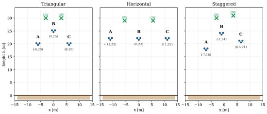
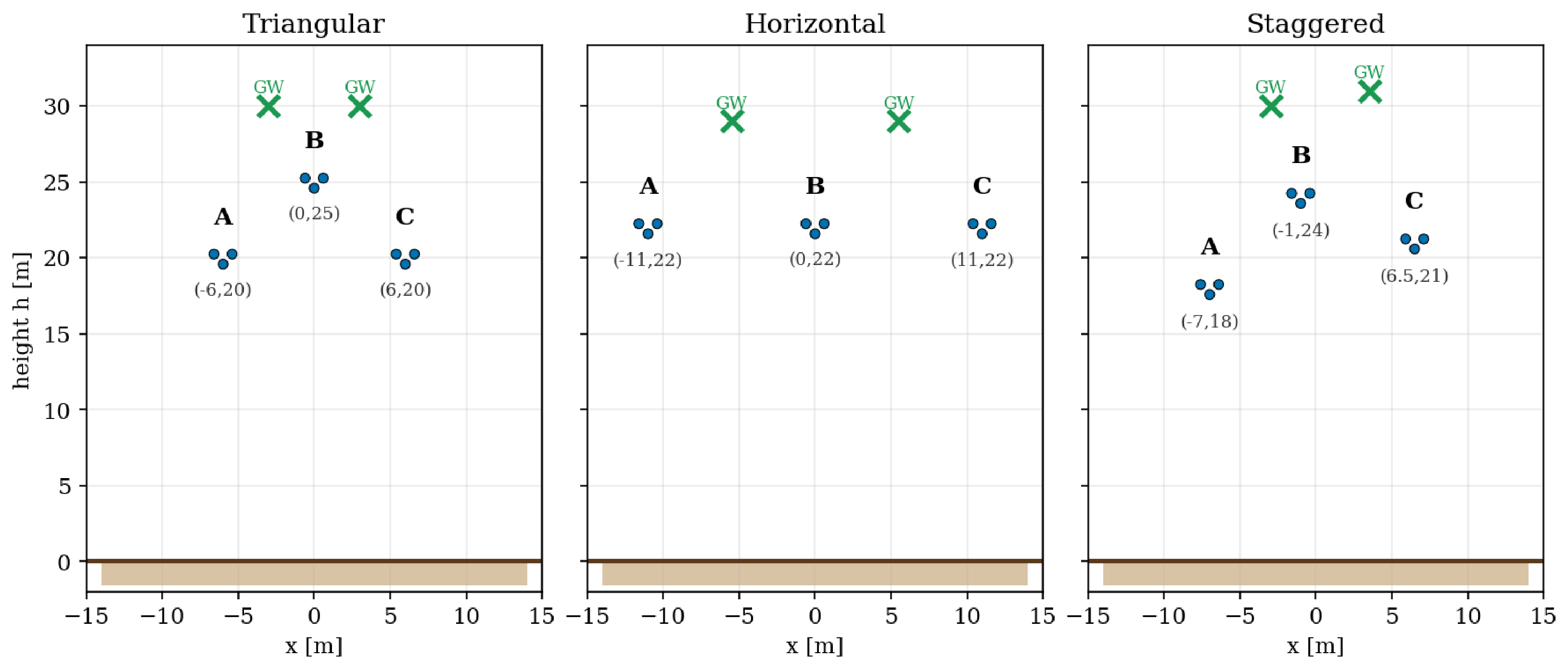
The four asymmetry parameters acquire a direct physical meaning when the line constants are computed from the tower geometry. To make this explicit, the reduced phase-domain matrix of a 400 kV single-circuit line was computed with OpenDSS (Carson earth-return model, 50 Hz) for the three tower arrangements shown in Figure 1: a triangular arrangement in which the centre phase is raised above the two outer phases, a horizontal (flat) portal arrangement with the three phases in one plane, and a staggered arrangement with no plane of symmetry. All three use the same conductors—a triple-bundle phase conductor and two ground wires—whose electrical data are listed in Table 4 and whose tower coordinates are given in Figure 1. The extended transform was then applied to each resulting matrix.
Figure 1.
The three 400 kV tower geometries (conductor coordinates in metres). A, B, C denote the phase conductors, each a three-conductor bundle; GW denotes the ground wires. Coordinate labels use the minus sign for negative positions.
Table 4.
Conductor data used for the OpenDSS line-constant calculations (50 Hz, Carson earth return). Each phase is a three-conductor bundle represented by its equivalent geometric mean radius (GMR) and equivalent capacitive radius.
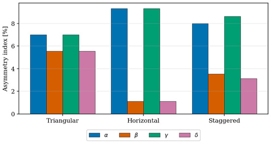
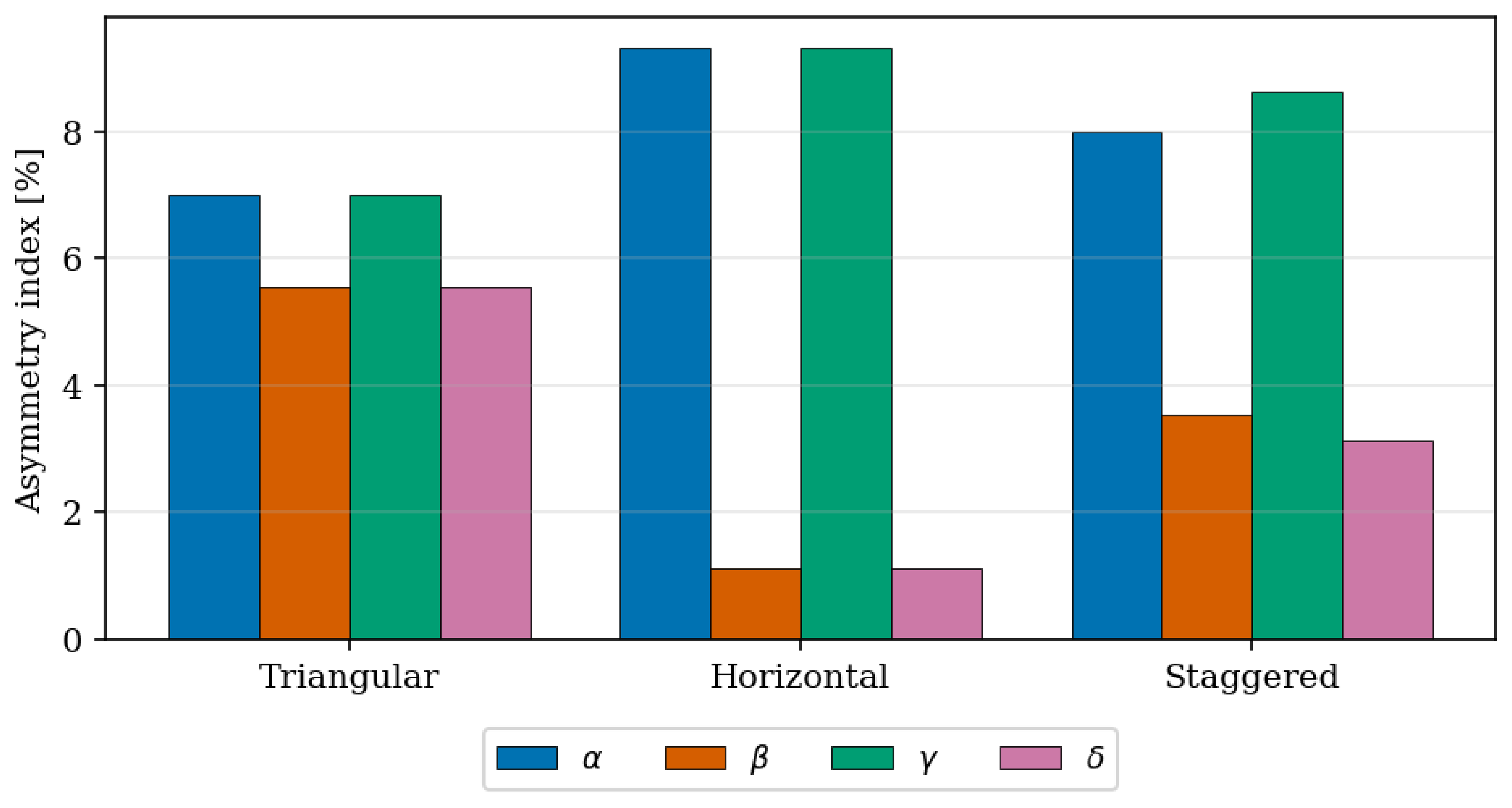
The results in Table 5 and Figure 2 reveal a clear structure. The pair measures the primary asymmetry, i.e., the deviation of the centre phase from the outer phases, while the pair measures the secondary asymmetry, i.e., the left–right imbalance between the two outer phases. A tower that possesses a vertical plane of symmetry (centre phase on the axis, outer phases mirrored) produces the exact numerical signature and ; this is observed for both the triangular geometry (, ) and the horizontal geometry (, ). The two tower types are nonetheless clearly distinguished by the parameters: the flat arrangement has a markedly larger “sum” asymmetry but a much smaller difference asymmetry . When the geometry has no symmetry plane—illustrated by a staggered arrangement with conductors at unequal horizontal offsets and heights—the degeneracy is broken and all four parameters become distinct (, , , ), confirming that the four indices carry independent geometric information rather than a redundant restatement of two quantities.
Table 5.
Extended-sequence asymmetry indices (% of ) for two typical 400 kV towers and a staggered (no-symmetry-plane) case, computed from tower geometry in OpenDSS for a 50 km section.
Figure 2.
Asymmetry indices for the three 400 kV geometries (50 km).
In summary, the four indices exhibit distinct dominant sensitivities: and (the pair) respond mainly to the primary asymmetry, namely the vertical offset of the centre phase relative to the outer phases, whereas and (the pair) respond mainly to the secondary asymmetry, the left–right imbalance between the two outer phases; within each pair the sum parameter (, ) reflects the combined self- and mutual-impedance deviation, while the difference parameter (, ) isolates the imbalance between them.
6.3. Extended Parameters in Terms of Phase-Domain Impedances
Substituting the definitions of and (Equation (5)) directly into Table 2 gives each extended parameter as a single linear combination of the six entries of :
where . The self-impedance entries () always carry weights of magnitude ; the mutual-impedance entries () carry weights of magnitude in the sum parameters and in the difference parameters.
6.4. Error Propagation Through the Extended Transform
Suppose every entry of is perturbed by an independent additive error :
Because is linear, the error in each extended parameter is obtained by applying the same rows of to the error vector :
Consider the special case for all (a uniform shift of every matrix entry):
For the asymmetry parameters, the self-impedance sums with equal weights are and , so:
All four asymmetry parameters are immune to a uniform common-mode error because their computation involves weights or which sum to zero. Only accumulates the full error (); and all four asymmetry parameters are unaffected.
7. Numerical Validation at the Fundamental Frequency
A 50 km overhead line with per-unit-length impedances computed by the Carson method [17] is used as the test case. The transposed equivalent has equal self-impedances and equal mutual impedances . The untransposed line retains the individual per-phase values, which differ due to unequal conductor heights and spacings.
7.1. Phase-Domain Matrices
The transposed and untransposed impedance matrices are, respectively:
7.2. Transposed Line
Applying the classical Fortescue transform yields a diagonal sequence matrix, confirming that a transposed line has no coupling between sequence networks:
The equality holds, as expected for any symmetric (reciprocal) .
Applying the extended transform gives:
All four asymmetry parameters vanish exactly, confirming backward compatibility with the classical result.
7.3. Untransposed Line
For the untransposed line, the classical sequence matrix is no longer diagonal. All three independent off-diagonal entries are non-zero, indicating cross-coupling between all sequence networks:
The diagonal entries remain equal because is still symmetric by reciprocity.
The extended transform yields four non-zero asymmetry parameters, while and are identical to the classical diagonal entries (Table 6):
Table 6.
Extended sequence parameters for the untransposed 50 km line.
The round-trip inverse recovers to machine precision (), confirming that the extended transform is lossless. This machine-precision agreement is an expected consequence of the non-singularity of and is reported only as a numerical consistency check on the implementation, not as a principal result.
7.4. Common-Mode Error Injection
To verify the immunity property analytically, a common-mode perturbation is added uniformly to every entry of :
where is the all-ones matrix. Applying the extended transform to gives (Table 7):
Table 7.
Extended sequence parameters for the perturbed untransposed 50 km line.
Comparing with shows that only is affected:
while the remaining five parameters are unchanged to machine precision. Since and a uniform perturbation shifts every entry of both and by , we have and , so:
For and the four asymmetry parameters, the same shift cancels in every expression.
7.5. Unbalance Factors from Extended Parameters
This section verifies numerically that all three off-diagonal entries of and the unbalance factors , can be recovered exactly from the extended parameters .
Inserting from Table 6 into Equations (15)–(17) recovers all three independent off-diagonal entries of (Table 8):
Table 8.
Reconstruction of off-diagonal sequence matrix entries from extended parameters versus direct computation.
All three values agree to machine precision. Note that the third entry is not captured by the unbalance factor characterisation (which uses only and ) but is fully determined by the extended parameters.
Computing and via both routes confirms agreement:
Both routes agree exactly. The extended representation encodes all information required for the unbalance factors, while additionally providing the third off-diagonal entry and enabling lossless round-trip reconstruction of .
7.6. Stochastic Perturbation Study
To complement the common-mode example, a Monte Carlo study was carried out in which the six independent entries of were perturbed independently in polar form. For each unique impedance entry, the magnitude was multiplied by with and the phase was shifted by an independent Gaussian perturbation with standard deviation expressed in degrees. The tested grid covered and , with 3000 trials per grid point.
Table 9 summarizes representative results. For the smallest-noise case, the sample means of the unbalance factors remained close to the deterministic baseline values, namely and , with standard deviations of and , respectively. Across the full tested grid, the inverse transform remained numerically exact, with the largest observed round-trip error equal to .
Table 9.
Summary of the stochastic perturbation study.
The same study also shows that the derived metrics do not respond equally to independent perturbations. Over the tested grid, the spread of was consistently larger than that of , which indicates that the negative-sequence coupling metric is more sensitive to entrywise uncertainty in this line example. The parameter-magnitude spreads show a similar ranking effect: the largest observed standard deviations were for , for , for , for , for , and for . Within the tested perturbation grid, increasing had a stronger influence than increasing . These results do not constitute a complete measurement-error model, but they do show that the proposed transform preserves exact algebraic reversibility while making it straightforward to study how independent entrywise perturbations propagate into the extended parameters and unbalance factors.
7.7. Line Length, the Distributed Model, and the Shunt Admittance
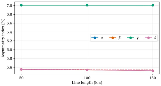
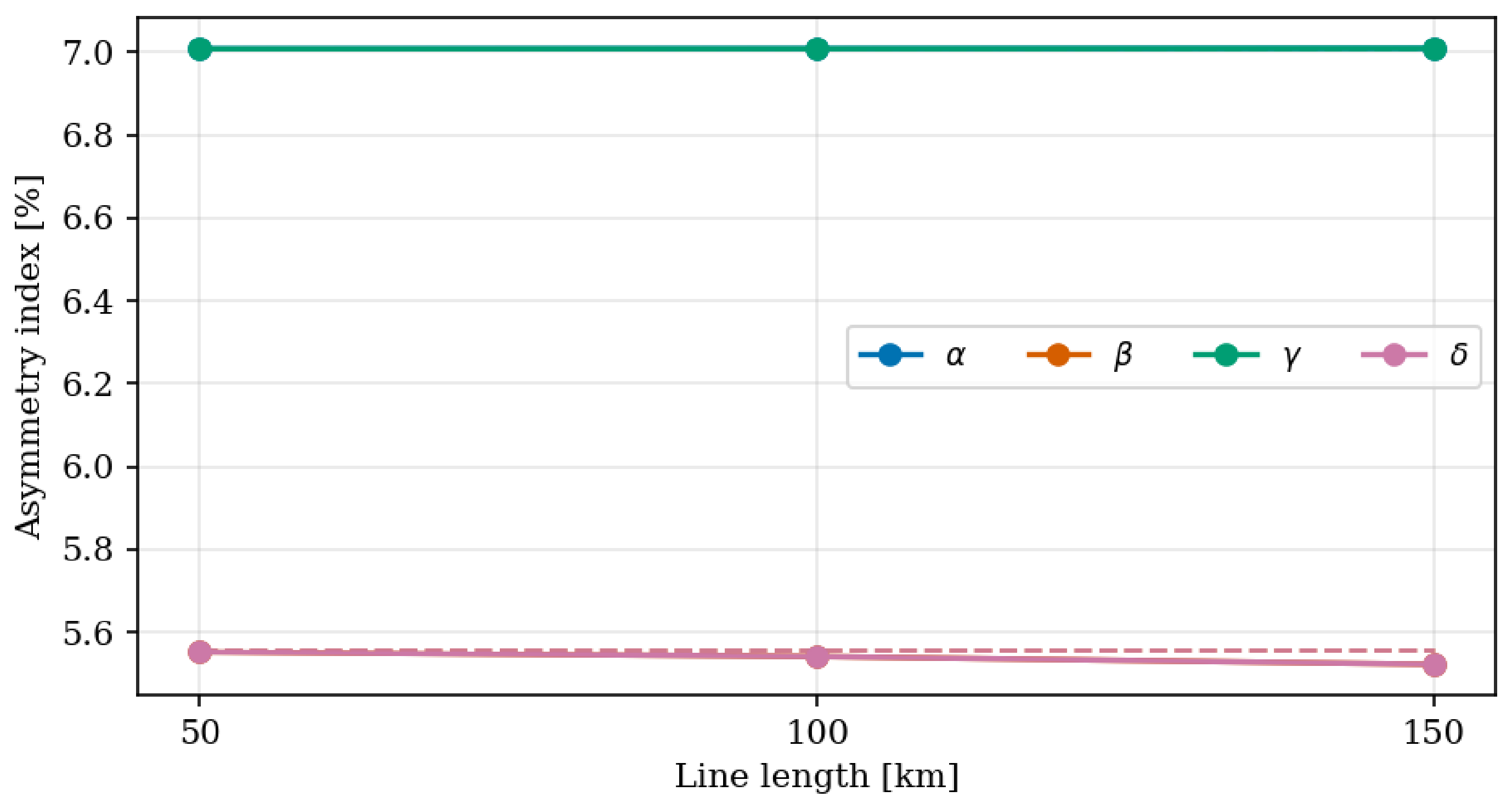
The numerical study above and the original example use a lumped series matrix at a single length. To examine the effect of line length, the triangular 400 kV geometry of Section 6.2 was evaluated at 50, 100, and 150 km, the upper range reported as feasible for untransposed operation. Two models were compared: the lumped series matrix , and the exact equivalent- series impedance obtained from the multiconductor two-port, with , which includes the full shunt admittance .
A useful property emerges for the lumped model: the asymmetry indices are ratios in which the common length factor cancels, so are exactly length-invariant (, at all three lengths). When the distributed model is used, the indices acquire a weak length dependence through the shunt admittance, but the relative change stays below about even at 150 km (Table 10, Figure 3). This quantifies the range over which the lumped-series characterisation of the asymmetry is adequate and justifies the simplification adopted in the rest of the paper. For the 50–150 km lengths considered, shunt reactors—which are external lumped compensation elements—do not alter the line matrix or its extended parameters, although they affect terminal behaviour; uncompensated operation is therefore representative for the present purpose. Frequency-dependent and broadband (transient) behaviour lies outside the intended fundamental-frequency scope and remains the domain of modal and electromagnetic-transient methods.
Table 10.
Length dependence of the asymmetry indices for the triangular 400 kV line (here and by tower symmetry). The lumped-series indices are length-invariant; the distributed model deviates by less than up to 150 km.
Figure 3.
Asymmetry indices (blue) and (orange) versus line length for the triangular tower: dashed lines, lumped-series model; solid lines, distributed model. For this symmetric tower and , so only and are plotted.
The shunt admittance itself is handled by exactly the same machinery. The capacitance matrix of a reciprocal line is symmetric and is transformed by the identical Fortescue similarity, so the same map applies to it without modification, yielding admittance counterparts with the same lossless round trip (< nF/km). For the triangular tower this gives and nF/km with and ; for the horizontal tower , nF/km with and . This is the reason the admittance was not treated as a separate development in the original manuscript—the transformation is the same—but the result is reported here for completeness.
7.8. Offline Measurement-Based Identification
The line is de-energised and isolated and its far end is earthed; the objective is the complete phase-domain matrix (six independent complex entries), from which , and follow through the extended transform. This can be carried out either with a three-phase source (Section 7.8.1) or with a single-phase source (Section 7.8.2). The two routes differ in the excitation and in where the current is read: the three-phase test applies voltage at the sending end and measures the short-circuit current at the earthed receiving end, whereas the single-phase test reads the injected current and the phase-to-earth voltages at the sending end.
7.8.1. Three-Phase Method
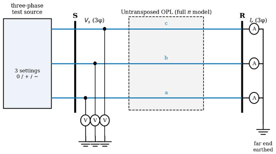
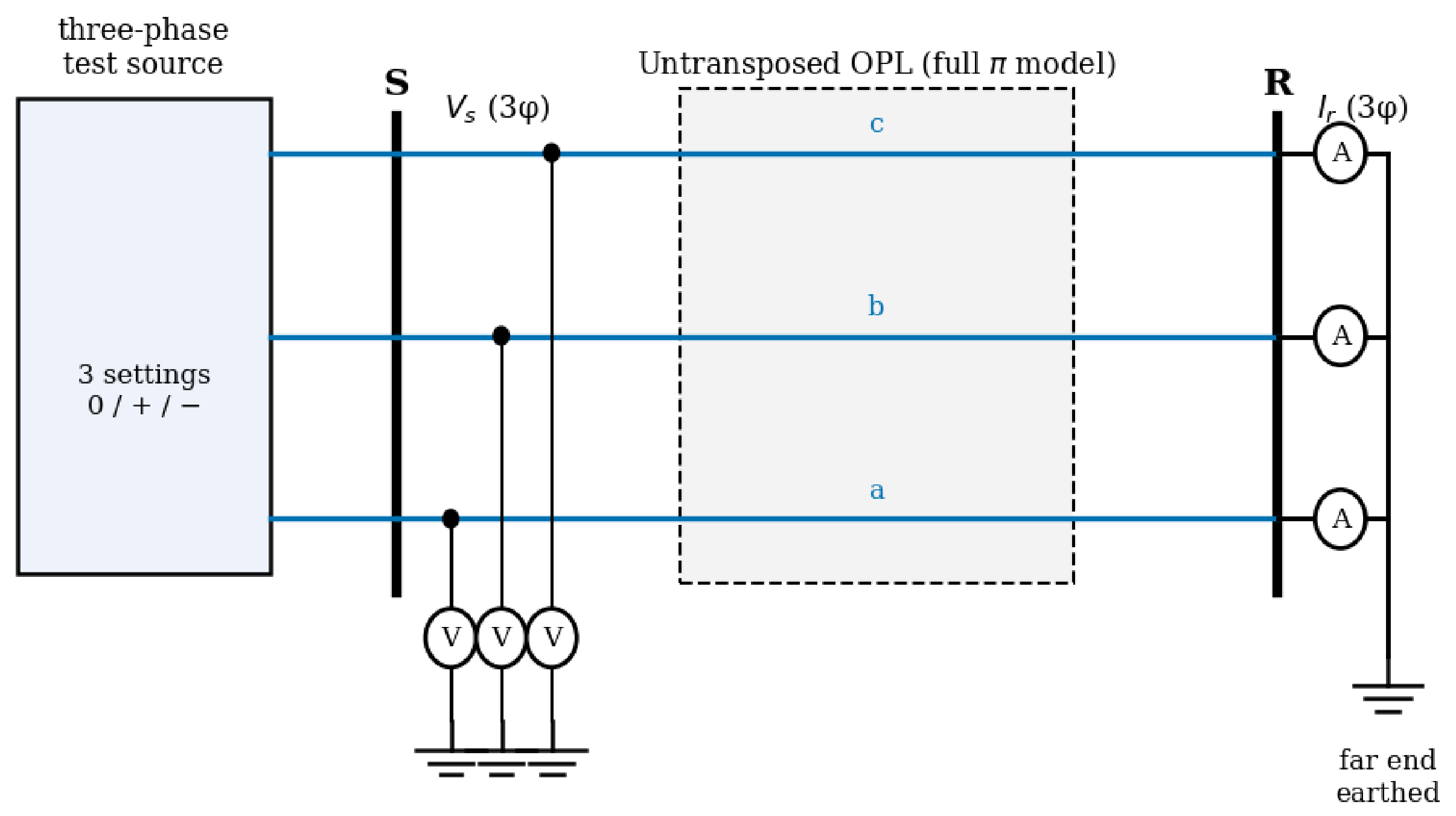
To demonstrate practical recoverability rather than asserting it, an offline (de-energised) staged test of the 50 km triangular line was simulated with an opendssdirect model that uses the full line description—the series impedance together with the complete shunt admittance (capacitance) matrix, i.e., the nominal- representation. The arrangement is shown in Figure 4. The receiving end is solidly earthed (three-phase short). A three-phase test source applies a known set of sending-end phase voltages , and the short-circuit current is measured at the earthed receiving end. Because the receiving end is shorted, the series (through) current dominates: for this line the sending-end shunt branch carries only about – of the through current, so essentially all of it reaches the earthed end and is captured by . With the receiving voltage forced to zero, the two-port reduces to , where is the series impedance. Three linearly independent excitations give and as matrices, the identified matrix is (symmetrised for reciprocity), and the extended transform is applied to obtain . Applying a known voltage and reading the short-circuit current is the natural offline procedure and is well conditioned: the applied sequence voltages form an orthogonal basis (condition number unity), whereas pure current injection would let part of the zero-sequence current return through the shunt capacitance and degrade the conditioning.
Figure 4.
Three-phase offline test: a known sending voltage is applied, the far end is shorted to earth, and the short-circuit current is measured. Here S and R are the sending and receiving terminals, V and A denote the voltmeter and ammeter, and a, b, c are the three phases.
This arrangement follows established offline practice. The conservative and consistent offline tests for AC transmission-line impedance are standardised in IEEE Std 1870-2019 [18], in which one- and three-phase voltage and current measurements on a de-energised, far-end-shorted line are the inputs for estimating the series impedance matrix; the same family of tests was applied experimentally to an overhead line in our earlier experimental study. In that practice the balanced three-phase test (all phases energised, far end shorted and earthed) yields the positive-sequence impedance , whereas bonding the three phases together and supplying them from a single-phase source against earth yields the zero-sequence impedance [18,19]. Only the zero-sequence test energises all three phases at the same voltage; the positive- and negative-sequence tests do not. The identification used here applies exactly this campaign—realised as three independent single-phase sources, equivalently a controllable three-phase source—but retains the complete identified matrix instead of collapsing each test to a single sequence scalar. The classical and are therefore obtained exactly as in the standard procedure, and the four asymmetry parameters follow from the same measurements at no additional cost.
An identifiability requirement follows directly from the structure of the problem and clarifies how the asymmetry parameters relate to the classical measurement of and . Each of and is a quantity obtained from a single matched excitation ( from a positive-sequence injection, from a zero-sequence injection). The four asymmetry parameters are and quantities describing differences between phases; they cannot be read from a single injection. Since a symmetric has six independent complex entries and each terminal excitation provides only three complex equations, a single excitation—however unbalanced—is underdetermined, and even two independent excitations leave the identification rank-deficient. Three linearly independent excitations are required and sufficient. They need not be the pure sequence sets; any independent set rich in zero- and negative-sequence content makes the asymmetry observable, while the zero/positive/negative triplet is simply the optimally-conditioned canonical choice (condition number unity). In other words, are obtained from the same three-phase tests already used for and , provided the full matrix is retained and the transform applied.
A worked example makes the procedure concrete. The three excitations are three three-phase voltage settings applied sequentially—one test after another, not at the same time—all at the same magnitude kV phase-to-earth. Setting 1 (zero sequence) drives the three phases at the same angle, on a, b and c. Setting 2 (positive sequence) drives , , . Setting 3 (negative sequence) drives , , . Collected as the columns of a matrix (in the order setting 1, 2, 3), the applied sending voltages and the measured short-circuit currents are
the three columns corresponding to the zero-, positive- and negative-sequence settings. Each column obeys , so the full matrix follows from a single inversion,
Applying the extended transform to the six independent entries of (the vector ) gives the six parameters directly (all in ):
The normalised indices are , , and . The classical and come out exactly as in the standard sequence tests, while the four asymmetry parameters are obtained from the very same three measurements.
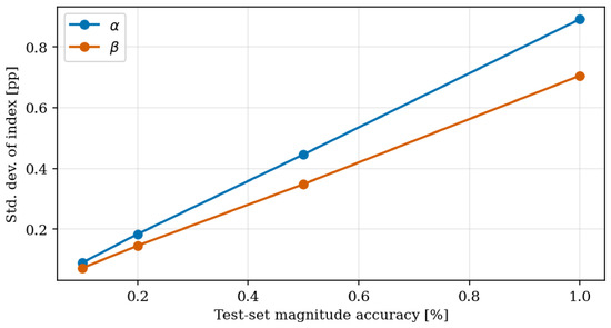
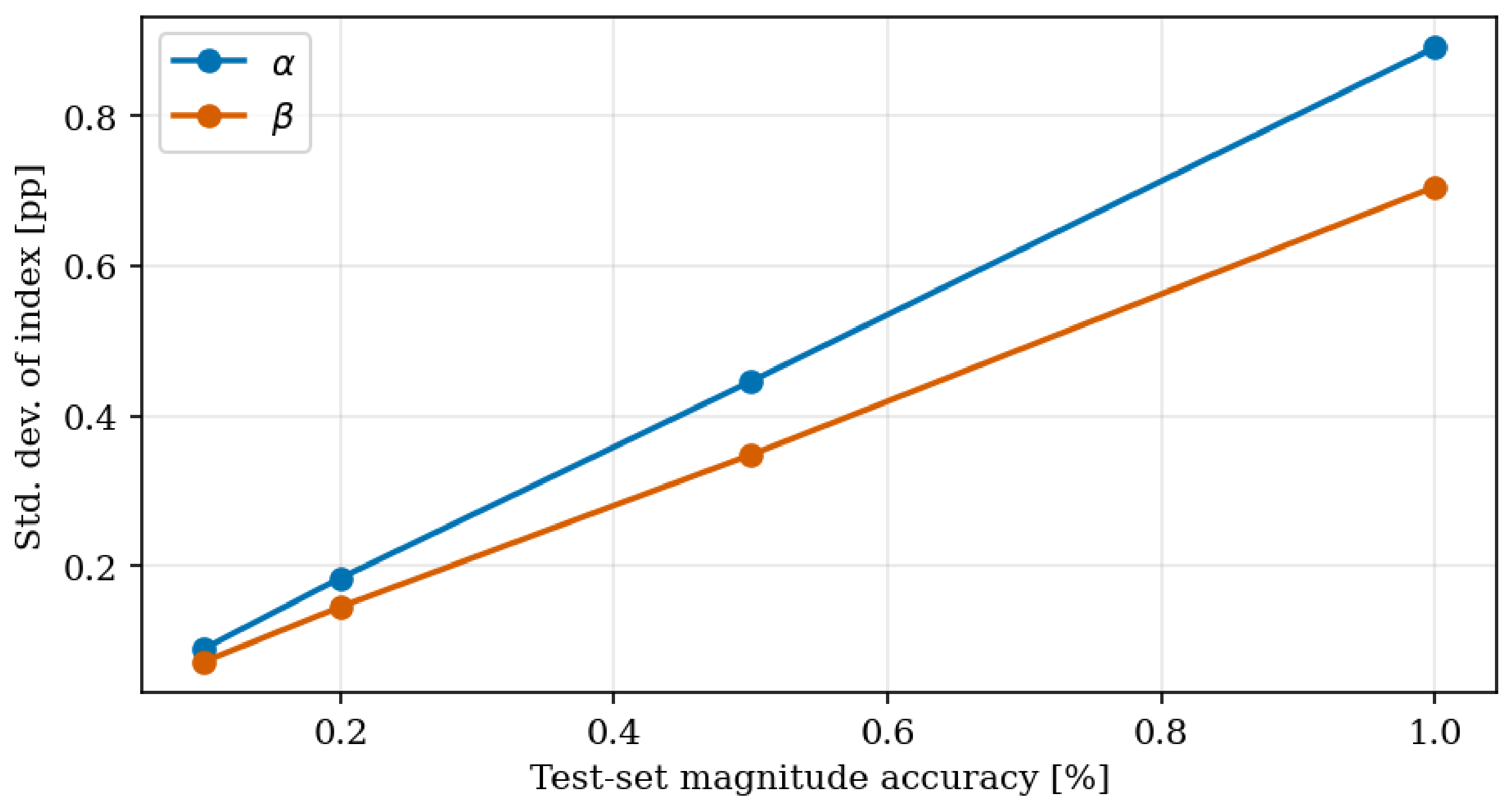
With noiseless data the identification is essentially exact (, the residual being the finite earthing resistance of the simulated short) and the indices are recovered to the same accuracy. Under realistic test-set instrument error (independent Gaussian magnitude and angle errors on every recorded phasor) the indices are recovered with the modest, quantified spread listed in Table 11 and plotted in Figure 5. For a magnitude/ class the standard deviations stay below percentage points on parameters of – (about relative); at / they remain below percentage points. For this symmetric tower and , so only and are reported; the sum parameter shows a slightly larger spread than the difference parameter .
Table 11.
Offline identification of the triangular 400 kV line: standard deviation (percentage points) of the recovered asymmetry indices over 5000 Monte Carlo trials, versus test-set accuracy class (magnitude/angle). For this symmetric tower and , so only and are listed.
Figure 5.
Spread of the recovered indices versus test-set magnitude accuracy (here , ).
This error analysis assumes a lumped-parameter line. As established in Section 7.7, that assumption changes the asymmetry indices by less than about up to 150 km—smaller than the instrument-induced spread already at the accuracy class—so it is adequate for the present measurement-error analysis; for longer lines, or where sub-percent accuracy is required, the distributed model of Section 7.7 should be used instead.
7.8.2. Single-Phase Method
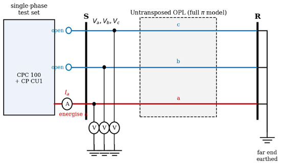
The same complete matrix—and therefore — can be obtained with a single-phase source, which is practically attractive because single-phase line test sets are common; for example, the OMICRON CPC 100 test system paired with the CP CU1 coupling unit is used for offline overhead-line parameter measurement. The governing requirement is unchanged: six independent scalar measurements are needed for the six independent entries of .
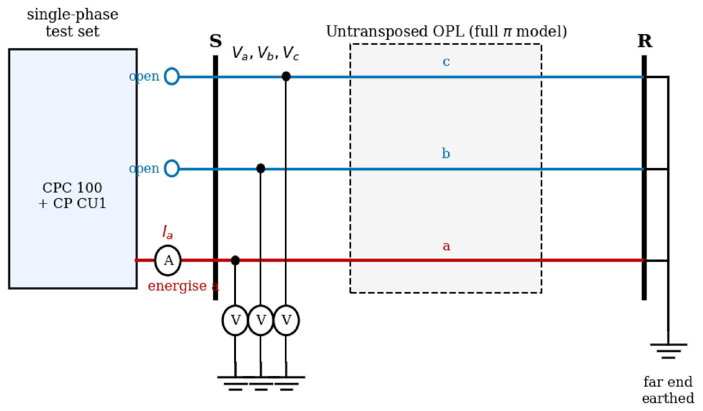
A convenient single-phase procedure is the column-at-a-time test of Figure 6. One phase is energised against earth, the other two phases are left open at the sending end, and the far end is earthed. Measuring the injected current together with all three sending phase-to-earth voltages yields one column of because with . Three such tests (energising a, then b, then c) complete the matrix; applying the extended transform to the triangular 400 kV line recovers to within about of the reference values.
Figure 6.
Single-phase column test: one phase energised, the other two open at the sending end, far end earthed. Here S and R are the sending and receiving terminals, V and A denote the voltmeter and ammeter, a, b, c are the three phases, and the open symbol marks the open-circuited sending terminals.
An equivalent route uses the classical single-phase tests directly: three phase-to-earth self measurements give the diagonal entries, and three phase-to-phase loop measurements give , from which the mutual terms follow as . The mutual coupling can also be probed by energising two phases and observing the third. If the third phase is earthed only at the far end and left open at the sending end it carries no current, but its induced open-circuit sending voltage equals ; if instead it is earthed at both ends it carries an induced current . Both quantities expose the mutual terms, and two excitations with different separate from . In every case the asymmetry parameters follow once the full has been assembled, which confirms that neither a balanced three-phase source nor any particular connection is essential—only a set of independent measurements sufficient to determine the six matrix entries.
8. Conclusions
This paper has presented the Extended Sequence Transform, a structured six-parameter representation of reciprocal untransposed overhead line impedance matrices.
The principal contribution is a linear mapping from the six independent entries of the phase-domain impedance matrix to six extended sequence parameters , together with its exact inverse . The transform is lossless in the sense that , so the full is recoverable to machine precision from the six parameters alone. The two classical sequence impedances and are preserved without modification, which makes the representation backward compatible with existing sequence-network analysis while collecting the asymmetry into four additional parameters.
All nine entries of the classical Fortescue sequence matrix are expressible as exact linear combinations of the six extended parameters, and the inductive unbalance factors and are completely determined by the four asymmetry parameters . Numerical validation at the fundamental frequency confirms exact round-trip reconstruction and exact agreement between unbalance factors computed from the classical and extended representations. The third independent off-diagonal entry , which is not captured by the standard unbalance factors alone, is also recovered directly.
The proposed transform is not a modal decoupling method and does not replace the full Fortescue matrix or frequency-dependent modal representations used in transient simulation. Its contribution is a compact parameterization in which the familiar pair is kept explicitly and the remaining asymmetry content is separated into four additional descriptors. This form is potentially useful in applications that need the complete reciprocal line matrix but also benefit from a small set of interpretable scalar parameters, including line modeling, comparison of untransposed configurations, and measurement-based parameter estimation.
These three uses are now supported by direct evidence rather than asserted. The comparison of untransposed configurations is demonstrated by OpenDSS calculations for two typical 400 kV towers, in which the four parameters relate to specific geometric features and discriminate between tower types (Section 6.2). Measurement-based estimation is demonstrated by a worked offline identification on a simulated line, including the requirement of three independent three-phase excitations and the resulting recovery accuracy under instrument error (Section 7.8). The length range of validity is established by the distributed-model study, which shows that the lumped-series asymmetry indices change by less than up to 150 km (Section 7.7). The exact invertibility of the transform should be understood as a prerequisite that makes these uses possible, not as the contribution in itself. The scope is correspondingly delimited: the development concerns reciprocal, passive line matrices at the fundamental frequency under a lumped-parameter treatment, and does not extend to rotating machines, frequency-dependent transient modeling, or modal-domain simulation. Field validation on measured data and integration with a specific estimation method remain the principal items of future work.
Author Contributions
Conceptualization, J.B. and M.C.; methodology, J.B. and M.C.; software, J.B.; validation, J.B. and M.C.; formal analysis, J.B. and M.C.; investigation, J.B. and M.C.; writing—original draft preparation, J.B.; writing—review and editing, J.B. and M.C. All authors have read and agreed to the published version of the manuscript.
Funding
This work was supported by the agency VEGA MŠVVaŠ SR under Grant No. VEGA 1/0380/26.
Data Availability Statement
The numerical data used for validation are contained within the article. The Python script used for the stochastic perturbation analysis can be made available by the corresponding author upon reasonable request.
Acknowledgments
The authors thank the reviewers for their constructive comments, which helped improve the technical positioning and validation of the manuscript. AI-assisted tools were not used in drafting any aspect of this manuscript beyond superficial language editing.
Conflicts of Interest
The authors declare no conflicts of interest.
Appendix A. Row-by-Row Derivation of M6
The rows follow from expanding Equation (5) and applying for each group k. All coefficients carry the factor from .
Group :
Group :
Group (using ):
Appendix B. Row-by-Row Derivation of M6−1
Apply : , , where are the plus/minus parameters of group k (Table 2). Then apply .
Recovering (rows 1–3):
Recovering (rows 4–6):
References
- Fortescue, C.L. Method of Symmetrical Co-Ordinates Applied to the Solution of Polyphase Networks. Trans. Am. Inst. Electr. Eng. 1918, XXXVII, 1027–1140. [Google Scholar] [CrossRef] [Scilit]
- Kiessling, F.; Nefzger, P.; Kaintzyk, U.; Nolasco, J.F. Overhead Power Lines: Planning, Design, Construction; Springer Science & Business Media: Berlin/Heidelberg, Germany, 2003. [Google Scholar]
- Survilo, J. Impact of Untransposed Power Lines. Power Electr. Eng. 2014, 32, 29–34. [Google Scholar] [CrossRef] [Scilit]
- EPRI. AC Transmission Line Reference Book—200 kV and Above, 3rd ed.; EPRI: Palo Alto, CA, USA, 2024. [Google Scholar]
- Ritzmann, D.; Wright, P.S.; Holderbaum, W.; Potter, B. A Method for Accurate Transmission Line Impedance Parameter Estimation. IEEE Trans. Instrum. Meas. 2016, 65, 2204–2213. [Google Scholar] [CrossRef] [Scilit]
- Wehenkel, A.; Mukhopadhyay, A.; Le Boudec, J.Y.; Paolone, M. Parameter Estimation of Three-Phase Untransposed Short Transmission Lines From Synchrophasor Measurements. IEEE Trans. Instrum. Meas. 2020, 69, 6143–6154. [Google Scholar] [CrossRef] [Scilit]
- Chase, S.; Sawai, S.; Kathe, A. Analyzing faulted transmission lines: Phase components as an alternative to symmetrical components. In Proceedings of the 2018 71st Annual Conference for Protective Relay Engineers, College Station, TX, USA, 26–29 March 2018; p. 19. [Google Scholar] [CrossRef] [Scilit]
- Dell’Olmo, J.; Gatta, F.M.; Geri, A.; Graziani, M.; Lauria, S.; Maccioni, M. Clarke Transform Based Fast Assessment of Switching Overvoltages in an MV Distribution Network. Electr. Power Syst. Res. 2022, 212, 108255. [Google Scholar] [CrossRef] [Scilit]
- Prado, A.; Pissolato, J.; Kurokawa, S.; Bovolato, L. Transmission line analyses with a single real transformation matrix-non-symmetrical and non-transposed cases. In Proceedings of the International Conference on Power Systems Transients (IPST’05), Montreal, Canada, 19–23 June 2005. [Google Scholar]
- Zhang, H.; Zhang, Q.; Gao, W.; Zheng, M. A Novel Transformation Matrix Based on Karrenbauer Transformation. Appl. Mech. Mater. 2014, 521, 260–263. [Google Scholar] [CrossRef] [Scilit]
- Nguyen, T.; Chan, H. Evaluation of modal transformation matrices for overhead transmission lines and underground cables by optimization method. IEEE Trans. Power Deliv. 2002, 17, 200–209. [Google Scholar] [CrossRef] [Scilit]
- Torrez Caballero, P.; Marques Costa, E.C.; Kurokawa, S. Modal decoupling of overhead transmission lines using real and constant matrices: Influence of the line length. Int. J. Electr. Power Energy Syst. 2017, 92, 202–211. [Google Scholar] [CrossRef] [Scilit]
- Faria, J.A.B.; Briceno, J.A. On the modal analysis of asymmetrical three-phase transmission lines using standard transformation matrices. IEEE Trans. Power Deliv. 1997, 12, 1760–1765. [Google Scholar] [CrossRef] [Scilit]
- Kurokawa, S.; Prado, A.J.; Pissolato, J.; Bovolato, L.F.; Daltin, R.S. Alternative proposal for modal representation of a non-transposed three-phase transmission line with a vertical symmetry plane. IEEE Lat. Am. Trans. 2009, 7, 182–188. [Google Scholar] [CrossRef]
- Tleis, N. Symmetrical components analysis of faulted three-phase networks containing voltage and current sources. Power Syst. Model. Fault Anal. 2019, 41–99. [Google Scholar] [CrossRef] [Scilit]
- Glover, J.D.; Sarma, M.; Overbye, T. Power Systems Analysis and Design; Cengage Learning: Singapore, 2007. [Google Scholar]
- Dommel, H.W. EMTP Theory Book; Microtran Power System Analysis Corporation: Fremont, CA, USA, 1992. [Google Scholar]
- IEEE 1870-2019; IEEE Guide for the Parameter Measurement of AC Transmission Lines. IEEE: New York, NY, USA, 2019.
- Cintula, B.; Eleschová, Ž.; Cenký, M.; Janiga, P.; Bendík, J.; Beláň, A. Three-Phase and Single-Phase Measurement of Overhead Power Line Impedance Evaluation. Energies 2021, 14, 6314. [Google Scholar] [CrossRef] [Scilit]

Disclaimer/Publisher’s Note: The statements, opinions and data contained in all publications are solely those of the individual author(s) and contributor(s) and not of MDPI and/or the editor(s). MDPI and/or the editor(s) disclaim responsibility for any injury to people or property resulting from any ideas, methods, instructions or products referred to in the content. |
© 2026 by the authors. Licensee MDPI, Basel, Switzerland. This article is an open access article distributed under the terms and conditions of the Creative Commons Attribution (CC BY) license.