


Abstract
Accurate electricity consumption forecasting is essential for the efficient planning and operation of modern power systems. The development of predictive models based on machine learning and deep learning strongly depends on the availability of well-documented and publicly accessible electricity consumption datasets. However, most existing databases are concentrated in Europe and North America and are typically focused on residential measurements obtained from smart meters, resulting in limited representation of equatorial regions. This work presents a structured review of public electricity consumption repositories, analyzing characteristics such as geographical coverage, temporal resolution, user type, and accessibility. Based on the limitations identified in the literature, a new electricity consumption dataset obtained from real measurements collected at distribution substations located in an equatorial region is presented. The dataset was organized through a systematic preprocessing workflow that included temporal standardization, construction of 48-h sliding windows, normalization, and stratified partitioning into training, validation, and test subsets. The descriptive statistical analysis confirms the consistency of the generated subsets and reveals differences between working-day and non-working-day consumption patterns. The proposed dataset provides a reproducible resource for the development and evaluation of multi-horizon electricity demand forecasting models, as well as for load analysis and energy management studies in equatorial regions.
1. Introduction
The sustained growth in electricity demand and the increasing complexity of modern power systems have driven the development of new methodologies for the analysis and prediction of energy consumption [1]. In recent years, the large volume of data generated by monitoring systems, smart meters, and electrical grid supervision platforms has enabled the application of advanced data analysis techniques, including machine learning and deep learning methods, with the aim of improving the planning, operation, and management of power systems [2].
Accurate electricity demand forecasting plays a fundamental role in the efficient management of energy generation, the operation of distribution networks, and energy planning in both the short and long term [3]. Several studies have shown that data-driven predictive models can significantly contribute to improving the stability of power systems, optimizing energy dispatch processes, and reducing operational costs associated with electricity generation and distribution [4,5].
The development and evaluation of these models largely depend on the availability of properly documented and accessible electricity consumption databases for the scientific community. Public repositories play a key role in enabling research reproducibility, comparison between different predictive models, and the execution of comparative studies across various methodologies. Over the past decade, several electricity consumption databases have been published for research purposes. Among the most widely used in the literature are UK-DALE [6], REDD [7], REFIT [8] and AMPds [9], which have served as benchmarks in numerous studies related to energy demand modeling and residential consumption analysis.
Despite the availability of these datasets, several relevant limitations still exist. First, many publicly available repositories focus primarily on household-level or smart meter consumption data, meaning they represent the behavior of individual users rather than the aggregated demand behavior at the level of electrical distribution networks. Second, most publicly available electricity consumption databases originate from Europe, North America, or parts of Asia, whereas databases from tropical and equatorial regions remain scarce.
Furthermore, a significant portion of publicly available open energy data consists of aggregated measurements from national power systems or high-voltage transmission networks, where operational information is more readily available. In contrast, datasets focused on low-voltage power distribution networks and at the feeder level remain considerably more limited, especially in equatorial regions. This lack of data hinders the development and evaluation of predictive models for real-world operating scenarios in power distribution systems [10,11].
Climatic, social, and economic conditions in regions near the equator can significantly influence electricity consumption patterns. Factors such as lower seasonal temperature variability, particular urban dynamics, and different energy consumption habits may generate load profiles that differ from those observed in temperate regions [12]. However, the scarcity of open databases from these regions limits the ability to study these characteristics and to develop predictive models adapted to such contexts.
For these reasons, expanding the geographical diversity of publicly available electricity demand datasets is essential to improve the representativeness of energy studies and to support the development of more robust and generalizable forecasting methodologies.
In this context, this work pursues two main objectives. First, a structured review of public electricity consumption databases used in the scientific literature is conducted, analyzing their main characteristics, geographic coverage, temporal resolution, and types of users represented. This review aims to provide an overview of the data resources currently available for electricity demand forecasting research and to facilitate their identification by the scientific community.
Second, this work presents and documents a new electricity consumption dataset from an equatorial region, constructed from real measurements obtained from electrical substations. The proposed dataset contains electricity consumption time series structured into 48 h prediction windows, allowing its use in the development and evaluation of multi-horizon electricity demand forecasting models. Additionally, the data acquisition, preprocessing, and structuring procedures are described in detail, including stages of data cleaning, temporal standardization, generation of temporal windows, and stratified partitioning into training, validation, and test sets, in order to ensure the reproducibility of experiments and facilitate its use in future research.
The rest of the article is organized as follows. Section 2 presents a review of public electricity consumption databases reported in the literature. Section 3 describes the proposed equatorial repository and the data acquisition environment. Section 4 details the dataset organization and preprocessing process. Section 5 describes the construction of the datasets used for the analysis. Section 6 addresses aspects related to dataset availability, procedural reproducibility, and ethical considerations. Section 7 presents a descriptive analysis of the proposed database. Finally, Section 8 presents the conclusions of the study, integrating the main implications, limitations, and future research directions.
2. Review of Public Electricity Consumption Databases
2.1. Importance of Databases in Electricity Consumption Forecasting
The prediction of electricity consumption depends largely on the availability of extensive, consistent, and representative time series that reflect the real behavior of energy demand. Machine learning models require large volumes of data to identify temporal patterns, capture nonlinear relationships, and generalize adequately to new operational scenarios [13].
In this context, databases constitute an essential component for the development of predictive models applied to electrical systems. The quality, diversity, and representativeness of the data directly influence model performance and their ability to adapt to different operating conditions of the electrical grid.
Furthermore, the availability of public repositories enables objective comparisons among different forecasting methodologies. This benchmarking process is fundamental for evaluating the performance of new algorithms and determining their applicability to real-world energy management problems [14].
Likewise, the electricity consumption datasets available in the literature present important differences in terms of geographical coverage, temporal resolution, aggregation level, and type of users represented. These characteristics determine the type of analysis that can be performed and the applicability of the predictive models developed using such datasets [15].
2.2. Criteria for Reviewing and Classifying Datasets
The comparison of electricity consumption datasets requires the consideration of technical criteria that make it possible to evaluate their scope, structure, and applicability in demand forecasting tasks [16]. In this study, the reviewed repositories were classified based on dimensions related to geographical coverage, climate type, aggregation level, temporal resolution, observation period, approximate sample volume, and public availability of the data.
The aggregation level is a fundamental criterion, since some datasets record consumption at the appliance or household level, while others provide aggregated information at the building, commercial customer, feeder, or electrical grid level. This difference directly conditions the type of problem that can be addressed, distinguishing between load disaggregation applications, residential analysis, aggregate demand forecasting, or operational planning of distribution networks [17].
Likewise, temporal resolution makes it possible to distinguish datasets oriented toward the analysis of high-frequency events, such as those with records every second or minute, from databases designed for hourly or daily forecasting. The observation period and the number of users, households, customers, or feeders included allow the temporal and spatial representativeness of each dataset to be assessed [18].
Finally, the public availability and aspects of documentation of each dataset were considered, since these aspects directly influence the reproducibility of studies and the possibility of benchmarking predictive methodologies as is show in Table 1.
Table 1.
Criteria used for the classification of electricity consumption datasets.
2.3. Quantitative Comparison of Public Electricity Consumption Datasets
Table 2 summarizes the main characteristics of the reviewed public repositories and makes it possible to compare their applicability with the dataset proposed in this study. Widely used datasets in the literature are included, such as UK-DALE, REDD, REFIT, AMPds, Pecan Street [19], and UCI Electricity Load Diagrams [20], due to their relevance in load disaggregation studies, residential analysis, consumption forecasting, and model benchmarking.
Table 2.
Quantitative comparison of public electricity consumption datasets.
As shown in Table 2, most of the widely used public databases are concentrated on residential measurements at the household or appliance level. These datasets are especially useful for load disaggregation studies, analysis of domestic energy behavior, and evaluation of smart metering algorithms. However, their direct applicability to demand forecasting tasks in distribution networks is limited, since they do not represent the aggregated behavior of electrical feeders or substations.
In contrast, data resources such as UCI Electricity Load Diagrams provide aggregated information from commercial and industrial customers, making them closer to aggregate load forecasting problems. Nevertheless, these data do not directly correspond to operational measurements of feeders within a real electricity distribution network.
The proposed dataset differs from the previous ones in three main aspects: first, it is built from real measurements at the feeder and substation level; second, it comes from an equatorial region, which is scarcely represented in existing public datasets; and third, it is specifically structured for multi-horizon forecasting tasks through 48 h temporal windows and stratified partitioning into training, validation, and test sets.
2.4. Characteristics and Limitations of Currently Available Datasets
The comparative analysis shows that public electricity consumption databases present important differences in terms of geographical coverage, temporal resolution, aggregation level, and operational applicability. Residential datasets such as UK-DALE, REDD, REFIT, AMPds, and Pecan Street offer high temporal resolution and make it possible to study consumption patterns at the household or device level. However, their scope is mainly oriented toward residential analysis and load disaggregation; therefore, they do not directly represent the aggregated dynamics of electricity distribution networks [21].
Another relevant limitation is the geographical concentration of the available datasets. Most of the reviewed repositories come from Europe and North America, regions with climatic conditions, consumption habits, and electrical infrastructure that differ from those observed in equatorial regions. This may limit the generalization capacity of predictive models trained exclusively with this type of data when applied to tropical or equatorial contexts.
In addition, there is lower availability of public datasets with real measurements at the feeder or substation level. Although open sources of aggregated demand at the national or transmission system level exist, operational data from distribution networks are usually less accessible due to technical, commercial, or security restrictions. This situation limits the development of predictive models aimed at planning, operation, and energy management in real distribution networks.
Finally, some databases present limited documentation regarding cleaning, normalization, temporal window construction, or splitting procedures into training, validation, and test subsets. This lack of standardization makes it difficult to reproduce studies and objectively compare forecasting methodologies.
In this context, the proposed dataset seeks to complement existing resources by publishing a real, documented, and structured dataset at the feeder and substation level, specifically oriented toward multi-horizon electricity demand forecasting in an equatorial region.
3. Contribution of a New Equatorial Electricity Consumption Dataset
3.1. Motivation and Contribution of the Proposed Dataset
The availability of public repositories focused on low-voltage electrical distribution networks remains limited compared to other levels of energy aggregation [22]. Although there are multiple data sources related to residential electricity consumption or aggregated demand at the national level, the availability of real operational measurements from distribution feeders and substations remains scarce in the scientific literature.
To contribute to addressing this issue, the present study introduces a new electricity consumption dataset obtained from real measurements collected at electrical substations located in Ecuador. Unlike many datasets available in the literature, which focus on individual residential consumption or building-level measurements, the proposed dataset incorporates aggregated measurements at the feeder and substation levels within a real electrical distribution network.
This approach makes it possible to capture the behavior of electricity demand under real operational conditions of the distribution system, providing a representative database that can be used for the development, training, and evaluation of predictive models focused on multi-horizon forecasting, load profile analysis, and energy management in electrical distribution systems.
Likewise, the proposed dataset includes information corresponding to the 2018–2022 period, including the interval associated with the COVID-19 pandemic, which allows for the analysis of operational variations and changes in electricity consumption patterns under different temporal and socioeconomic contexts.
3.2. Study Environment and Geographical Location
The dataset used in this study was constructed from measurements obtained at electrical substations located in different areas of Ecuadorian territory, which are part of the national electricity distribution system. These substations operate under real load conditions and supply different types of consumers, including residential, commercial, and light industrial sectors.
The substations considered include Alluriquín, Quito, El Carmen, Patricia Pilar, and La Concordia. These areas present relevant differences in terms of altitude, urban–rural environment, and climatic conditions, making it possible to capture heterogeneous demand profiles within an equatorial region. In particular, Quito represents a high-altitude Andean urban area, while Alluriquín, El Carmen, Patricia Pilar, and La Concordia are located in lower-altitude areas, with greater tropical influence and the presence of peri-urban, rural, and productive sectors.
Table 3 summarizes the main geographical and operational characteristics of the substations considered in the study. This characterization makes it possible to contextualize the spatial variability of the dataset and justify its usefulness for analyzing electricity demand patterns in equatorial distribution networks.
Table 3.
General characteristics of the substations considered in the dataset.
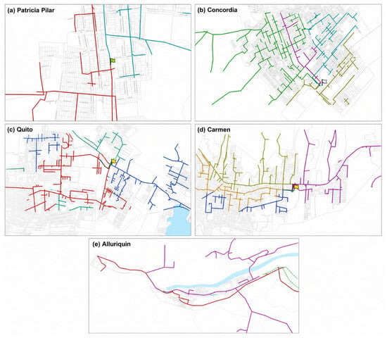
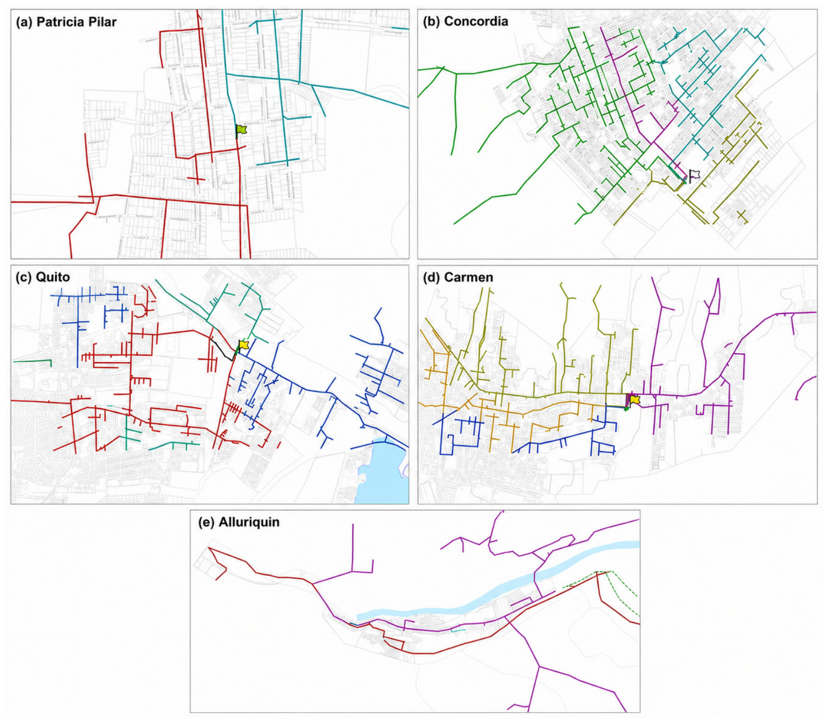
The geographical distribution of the substations and feeders included in the dataset is presented in Figure 1, which shows the location of the measurement points within the Ecuadorian electricity distribution system. This map makes it possible to visualize the spatial arrangement of the analyzed substations and provides geographical context for the subsequent interpretation of the data.
Figure 1.
Geographical location of the electrical substations and distribution feeders used in the dataset within the Ecuadorian electrical system: (a) Patricia Pilar; (b) Concordia; (c) Quito; (d) Carmen; and (e) Alluriquín. Colored flags identify the electrical substations, whereas colored lines represent the distribution feeders associated with each sub-station.
The inclusion of multiple feeders from different substations makes it possible to capture heterogeneous demand profiles. This diversity is especially relevant for the development of robust predictive models, since it incorporates consumption patterns associated with urban, peri-urban, and rural areas, as well as different climatic and altitudinal conditions within Ecuadorian territory.
3.3. Data Acquisition Infrastructure
The data used in this study were acquired through a monitoring and management infrastructure for electrical networks based on modern automation systems. This infrastructure integrates different functional levels that allow capturing, transmitting, storing, and managing operational information of the electrical distribution system.
At the supervision level, a SCADA system (Supervisory Control and Data Acquisition) is used, responsible for the real-time acquisition of electrical variables measured in the field. The SCADA system allows continuous monitoring of the operational status of substations and feeders, as well as recording electrical measurements from devices installed in the network [23].
The data collected by the SCADA system are subsequently integrated into an ADMS (Advanced Distribution Management System), specifically the EcoStruxure™ ADMS version 3.4.2 software, which provides advanced tools for the management and analysis of the electrical network. This system allows performing operational analyses, scenario simulations, and decision-making support within the distribution system [24].
The overall data acquisition and management architecture is based on the international IEC 61850 standard, widely used in electrical substation automation systems. This standard defines communication protocols and data models that enable interoperability between different measurement devices and control systems within the electrical network.
Electrical measurements are recorded using high-precision electronic devices manufactured by Schneider Electric (Rueil-Malmaison, France) from the PowerLogic ION Series family, including models from the ION 7000, ION 8000, and ION 9000 series. These meters receive signals from current transformers (CT) and potential transformers (PT), which allow measuring the three-phase electrical variables present in the distribution feeders.
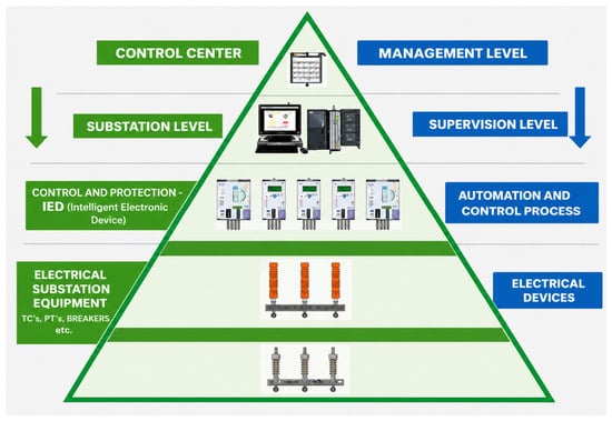
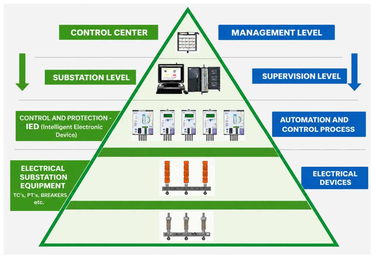
The general data acquisition flow, from field measurement devices to electrical network management systems, is illustrated in Figure 2, where the main levels of the supervision and management architecture used in the study are presented.
Figure 2.
Hierarchical architecture of the SCADA–ADMS system used for the acquisition and management of electrical data in the distribution system [25].
3.4. Dataset Description
3.4.1. Data Source
The final dataset corresponds to aggregated measurements at the feeder level, allowing the representation of the collective behavior of multiple users connected to each distribution circuit. This characteristic differentiates the proposed dataset from other widely used datasets in the literature, which usually focus on household- or device-level measurements.
3.4.2. Measured Electrical Variables
The database includes a set of fundamental electrical variables. Among the main recorded variables are those in Table 4.
Table 4.
Variables recorded in the original dataset.
These variables on Table 4 allow describing the operational state of the electrical system and constitute the basis for analyzing demand behavior. In particular, the total three-phase apparent power variable (kVA_tot) was used as the main variable for constructing the time series used in forecasting tasks, due to its ability to represent the electrical load behavior in an integrated manner.
Additionally, the dataset includes auxiliary variables related to the spatial and operational identification of the records, such as feeder, substation, number of customers, and geographic coordinates. These complementary variables enrich the descriptive analysis of the dataset and facilitate its traceability within the electrical distribution system.
3.4.3. Temporal Sampling Frequency and Observation Period
Electrical measurements were originally recorded with a temporal resolution of 15 min, allowing the capture of relevant operational variations in electricity consumption throughout the day. This type of temporal resolution is common in SCADA systems and provides an adequate level of detail for analyzing demand behavior.
Subsequently, as part of the dataset organization and preprocessing process described in the following sections, these measurements were standardized to an hourly resolution in order to reduce data redundancy and facilitate the training of multi-horizon predictive models. To perform this temporal standardization, only the record corresponding to the exact hour (HH:00) was selected from each hourly block, discarding observations recorded at 15, 30, and 45 min past each hour. This procedure allowed constructing a uniform hourly time series while maintaining temporal consistency.
The transformation from a 15 min temporal resolution to an hourly resolution preserves the main electricity consumption trends while reducing data volume and simplifying the structure of the time series used in predictive modeling. However, the published dataset also retains the original 15 min resolution records so that future studies can use the full temporal resolution or alternatively generate equivalent datasets by applying the same methodological procedure to the records corresponding to minutes 15, 30, and 45 of each hour. This approach would allow construction of additional dataset variants and a significant increase in the number of samples available for predictive modeling tasks.
Regarding the observation period, the dataset covers records from January 2018 to December 2022, providing a sufficiently broad temporal coverage to capture short- and medium-term variations in electricity consumption behavior. This interval also includes the period corresponding to the COVID-19 pandemic, an event that significantly altered certain electricity consumption patterns and therefore constitutes a relevant characteristic of the temporal context represented in the dataset.
4. Dataset Organization and Preprocessing
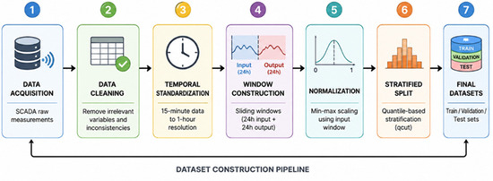
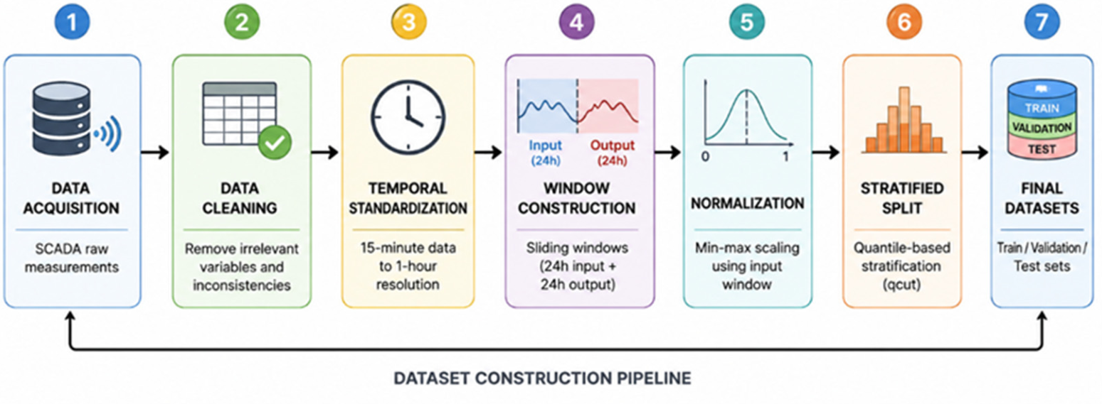
The dataset organization and preprocessing process was carried out through a structured sequence of five main stages aimed at ensuring the quality, consistency, and usefulness of the data for predictive modeling. These stages include: (i) the removal of irrelevant variables and cleaning of inconsistent records, (ii) the temporal standardization of the series at an hourly resolution, (iii) the construction of input and output time windows for multi-horizon forecasting, (iv) data normalization to reduce scale effects, and (v) record stratification to ensure a balanced distribution across the training, validation, and test sets. Each of these stages is described in detail below.
In order to provide an overview of the methodological procedure followed for the construction of the dataset, Figure 3 presents a summarized scheme of the processing workflow applied from the acquisition of the original measurements to the final generation of the training, validation, and test subsets.
Figure 3.
General methodological flow for the organization and preprocessing of the electricity consumption dataset.
4.1. Cleaning of Irrelevant Variables
The original dataset obtained from the SCADA system includes multiple electrical variables associated with feeder operation, such as voltages, currents, active power, reactive power, and three-phase apparent power.
However, not all these variables are necessary for the specific objective of this study, which focuses on forecasting aggregated electricity consumption at the feeder level. For this reason, an initial filtering stage was performed to select only those variables relevant for the analysis.
In particular, priority was given to the use of the total three-phase apparent power variable (kVA_tot) as a representative indicator of overall electricity demand behavior. This variable simultaneously integrates the effects of active and reactive power in the electrical system and is widely used in load modeling studies in distribution networks.
During this stage, the presence of missing values, incomplete records, or inconsistencies in the time series was also verified. Records containing null values, temporal discontinuities, or measurement inconsistencies were removed to ensure the integrity of the time series used in subsequent processing stages.
4.2. Temporal Standardization
The original electrical measurements were recorded with a temporal resolution of 15 min, which generates four records per hour for each feeder. Although this level of detail makes it possible to capture fine operational variations in the electrical system, it also introduces redundancy when the objective is to model consumption patterns at larger temporal scales.
In order to simplify the structure of the time series and reduce the volume of data without losing relevant information about demand behavior, a temporal standardization process was carried out, oriented toward working with hourly records.
Instead of averaging the four intra-hour measurements, only the records corresponding to each exact hour were retained, thus obtaining a uniform hourly time series. This approach makes it possible to preserve consumption dynamics at the hourly scale, reduce information redundancy, and decrease the computational cost associated with training predictive models. In particular, it was observed that variations among measurements recorded within the same hour were generally small, while the most representative changes in load profiles tended to appear at the hourly scale.
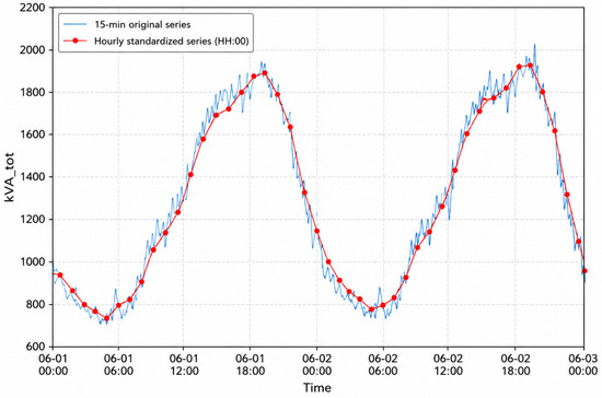
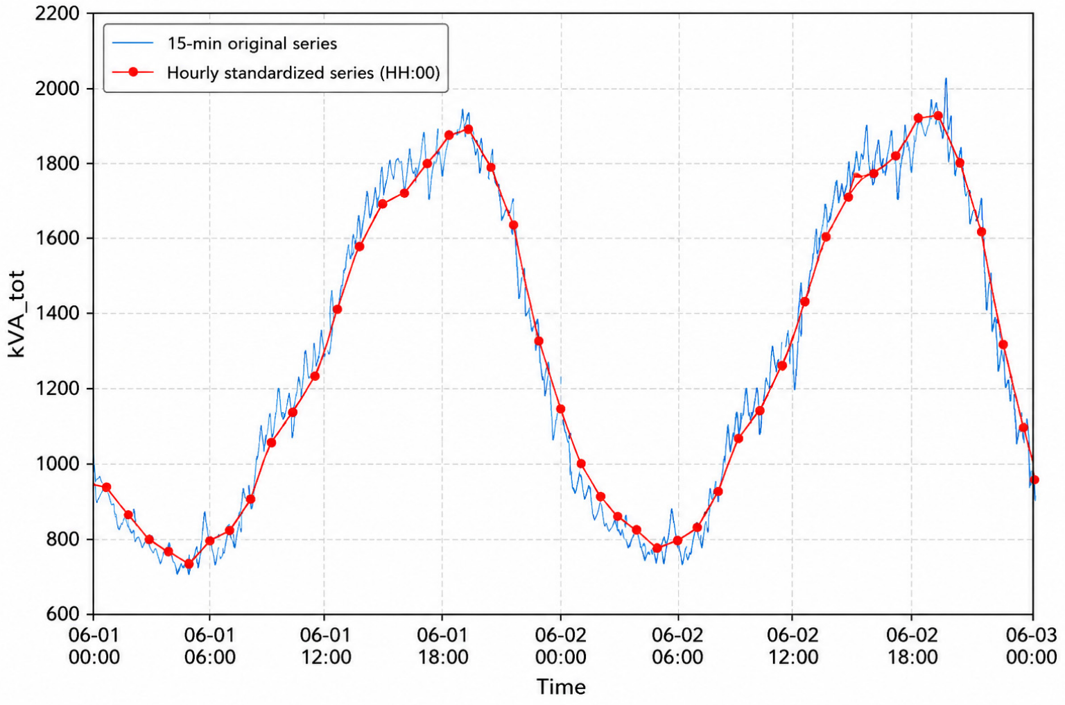
To support this decision, a visual comparison was performed between the original series with 15 min resolution and the hourly series obtained by selecting records at the exact hour. Figure 4 shows a representative example for one feeder during a 48 h period, where it can be observed that the hourly series preserves the main trend of the daily load profile, while the intra-hour measurements show minor variations with respect to the general behavior. This evidence supports the use of hourly resolution for constructing the multi-horizon forecasting dataset.
Figure 4.
Comparison between the original kVA_tot series with 15 min resolution and the series standardized to hourly resolution by selecting records at the exact hour.
Hourly resolution was selected because the main objective of the dataset is the development of multi-horizon electricity demand forecasting models at the operational scale of distribution systems. In this context, hourly representation makes it possible to adequately capture daily load profiles and general consumption patterns, maintaining a balance between the level of temporal detail and computational complexity. In addition, the use of hourly data facilitates comparison with numerous electricity demand forecasting studies reported in the literature.
Although the use of the series corresponding to minutes 15, 30, and 45 could be considered as a data augmentation strategy, this alternative was not applied in this study.
Likewise, the records were ordered chronologically according to the feeder and the corresponding timestamp, ensuring the temporal coherence required for the subsequent construction of continuous observation sequences.
4.3. Construction of Temporal Windows
Once the time series were organized, 48 h temporal windows were constructed, which constitute the basic units of analysis used in the dataset.
For an hourly time series of electricity consumption associated with a given feeder, the sequence is defined as:
where (xt) represents the hourly value of the variable (kVA_tot) at time (t), and (T) corresponds to the total number of observations available for that feeder.
Each temporal window was constructed from two consecutive segments: a 24 h input segment and a 24 h output segment. Formally, for an initial position (i), the window is defined as:
where (Xi) represents the input vector used by the predictive model, and (Yi) corresponds to the future horizon to be estimated. In this way, each sample in the dataset is represented as the pair:
with a total length of 48 consecutive hourly values.
To ensure the temporal coherence of these windows, it was verified that the records included in each vector maintained strict hourly continuity. Data blocks presenting interruptions or inconsistencies in the temporal sequence were discarded.
Additionally, an independent test set was defined by extracting vectors without temporal overlap, preventing the models from being evaluated with data that shared temporal information with those used during training.
Subsequently, as a temporal data augmentation strategy, the remaining set was expanded by generating shifted windows with a one-hour step. In this case, two consecutive windows are constructed as (Wi) and (Wi + 1), sharing part of the temporal information while preserving the chronological coherence of the series. This strategy made it possible to increase the number of examples available for model training without introducing inconsistencies into the time series.
4.4. Normalization
Electricity consumption time series may present significantly different amplitudes depending on the feeder considered. These differences can affect the training process of machine learning models, especially in neural network-based architectures, because variables with larger magnitudes may dominate the learning process.
To reduce this effect, a min–max normalization procedure was applied individually to each temporal window. In particular, the normalization parameters were calculated exclusively from the 24 h input segment, in order to avoid the use of future information during preprocessing.
The applied transformation is defined as:
where (xt) represents the consumption value at time (t), (Xi) corresponds to the input vector of window (i), (min(Xi)) and (max(Xi)) represent the minimum and maximum values observed in the 24 h input segment, and ε is a small term used to avoid division by zero in windows with constant values.
With this procedure, the values corresponding to the input segment are scaled within the interval ([0,1]). The values of the output horizon (Yi), corresponding to the future 24 h to be predicted, were normalized using the same parameters (min(Xi)) and (max(Xi)) calculated from the input. This criterion is fundamental from a methodological perspective, since in a real forecasting scenario future values are unknown and, therefore, should not be used to estimate normalization parameters.
As a consequence, the normalized values of the output horizon are not necessarily restricted to the interval ([0,1]), since future demand may exceed the maximum or fall below the minimum observed during the 24 h input segment. This behavior does not represent a methodological inconsistency, but rather an expected consequence of avoiding information leakage. Furthermore, in time series forecasting tasks, the output layer of the models usually uses a linear activation function, so the predictions are not bounded to a fixed interval. For this reason, the possible presence of normalized values outside ([0,1]) does not limit the application of the dataset in forecasting models, as long as the architecture used employs an unbounded output and the corresponding denormalization is applied to interpret the results in real units.
4.5. Data Stratification
To ensure a balanced distribution of electricity consumption patterns across the different subsets of the dataset, a stratification process based on the level of electricity demand was implemented.
Each time window was labeled using the average electricity consumption during the 24 input hours. Specifically, the variable used to define the strata was the average electricity consumption of the kVA_tot variable corresponding to the 24 input hours of each time window, since this variable represents the overall demand level associated with each temporal vector.
Based on this criterion, different electricity demand strata were defined by discretizing the mean kVA_tot values computed over the 24 h input window into representative intervals. Specifically, the strata were generated using quantile-based discretization (qcut), dividing the distribution of the mean input demand into ten groups with similar numbers of samples. This approach ensured a balanced representation of different electricity demand levels across the training, validation, and test subsets.
Subsequently, a stratified split was applied to divide the data into three main subsets: training set, validation set, and test set.
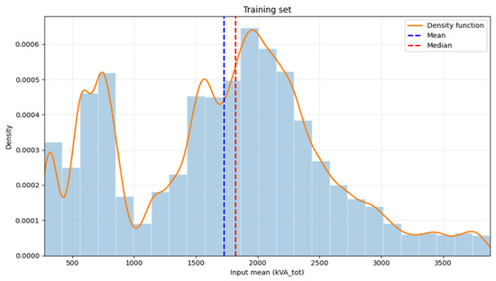
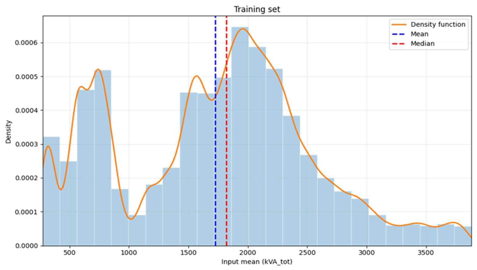
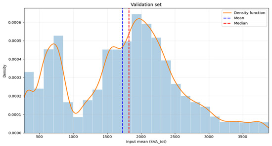
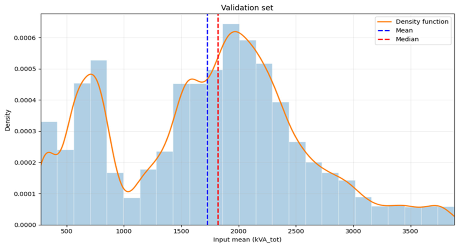
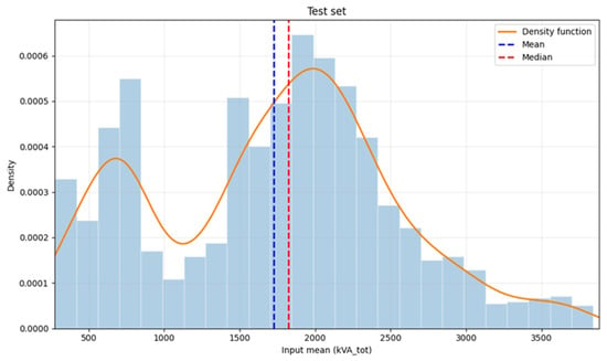
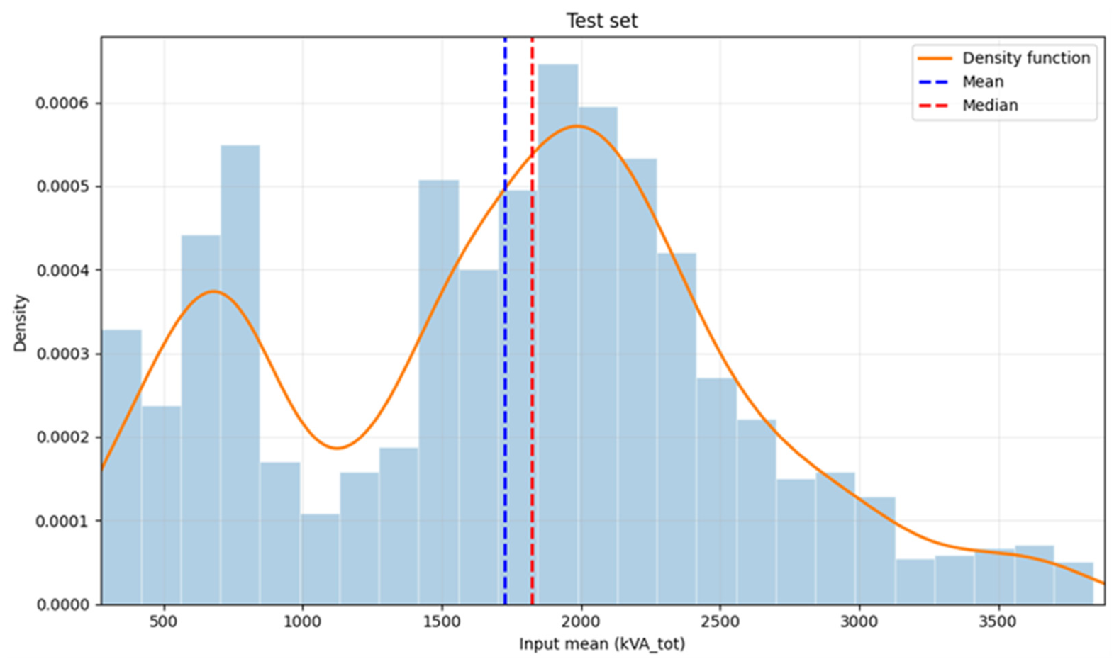
To visually verify the consistency of the stratification process, the distributions of the mean input demand, computed over the 24 h input window, were compared across the three generated subsets using histograms and density curves. Figure 5, Figure 6 and Figure 7 present the distributions for the training, validation, and test sets, respectively, using a common horizontal scale to facilitate comparison. In each figure, the mean and median values are also indicated to characterize the central tendency of the corresponding distribution.
Figure 5.
Distribution of the training dataset, showing histogram, density curve, and positions of the mean, median, and bimodal distribution.
Figure 6.
Distribution of the validation dataset, showing histogram, density curve, and positions of the mean, median, and bimodal distribution.
Figure 7.
Distribution of the test dataset, showing histogram, density curve, and positions of the mean, median, and bimodal distribution.
The results show that the three distributions have very similar shapes, which confirms that the stratified split adequately preserves the statistical representativeness of the electricity demand levels across the different subsets of the dataset.
The comparison of the probability distributions corresponding to the training, validation, and test sets reveals a persistent bimodal behavior, characterized by the presence of two clearly differentiated local maxima in the density curves. This behavior reflects the existence of different operating regimes within the electrical distribution system.
The first mode is mainly associated with base-load conditions, linked to periods of lower electricity demand, typically observed during nighttime and the early hours of the day. In contrast, the second mode corresponds to higher-demand conditions, associated with periods of greater economic and social activity, especially during working and evening hours.
Likewise, the high similarity observed among the distributions of the training, validation, and test subsets confirms that the stratified partitioning procedure adequately preserves the structural complexity and diversity of electricity consumption patterns present in the original dataset. In this context, the relatively close positions of the mean and median reflect the recurrent alternation between both demand regimes, providing a balanced representation of different operating states for the training and evaluation of predictive models.
5. Dataset Construction
Once the organization and preprocessing of the time series were completed, the construction of the final datasets used in the study was carried out [26].
As a result of this process, two main dataset configurations were generated: a base dataset, representing the general behavior of electricity consumption, and a specific dataset for non-working days, aimed at analyzing demand patterns during holidays and weekends.
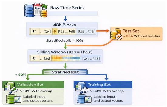
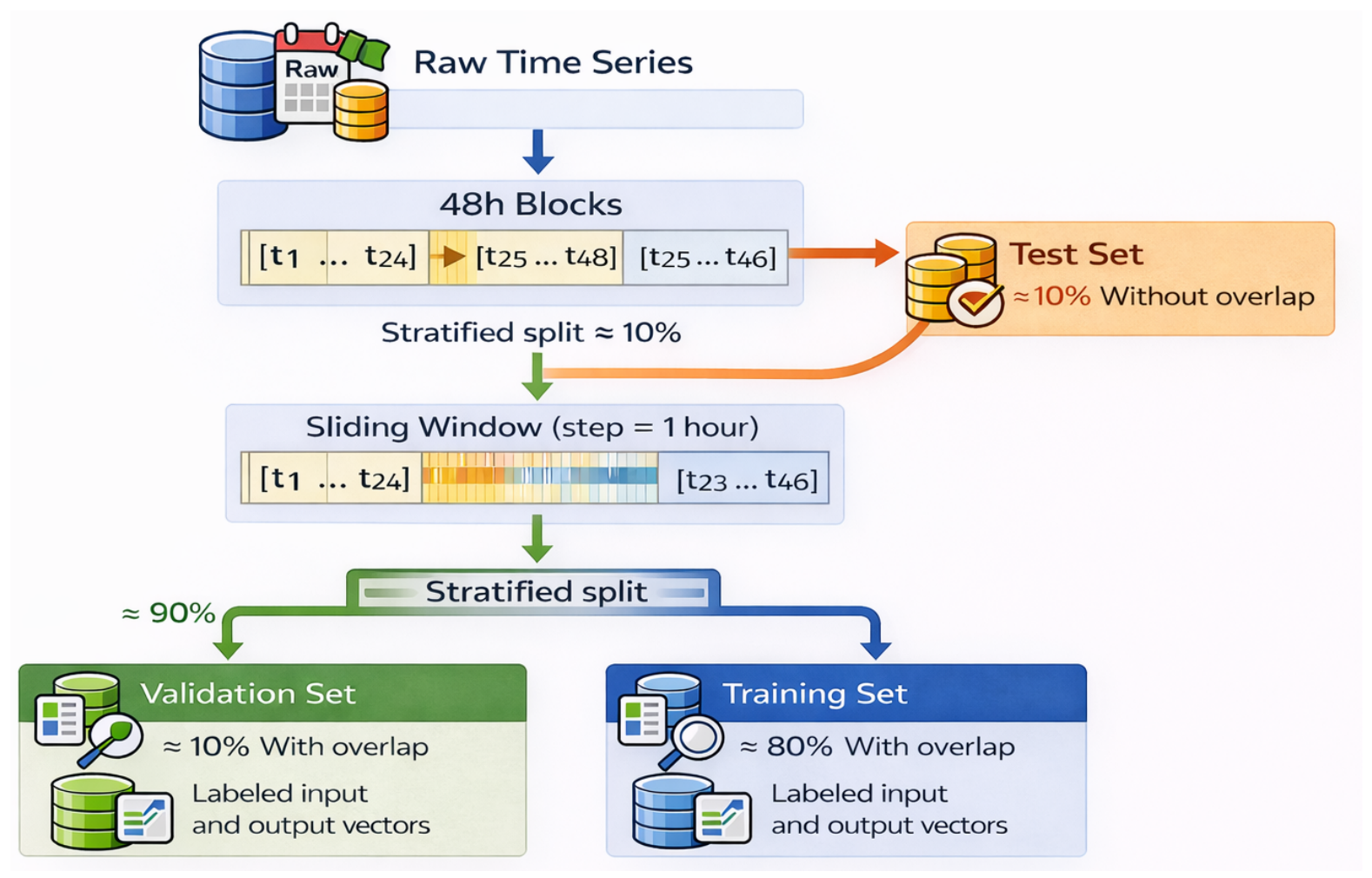
The general procedure followed for constructing the subsets is summarized in Figure 8. It shows, first, the preprocessed and labeled time series; then, the generation of temporal windows using a sliding window scheme with a one-hour step; followed by the extraction of an independent test set without temporal overlap; and finally, the stratified partitioning of the remaining dataset based on the mean value of the kVA_tot variable to obtain the training and validation subsets.
Figure 8.
Methodological workflow for constructing dataset subsets from preprocessed time series, showing the generation of sliding windows with a one-hour step, the extraction of a non-overlapping test set, and the stratified partitioning of the remaining dataset into training and validation sets based on the mean kVA_tot value. The ellipsis (…) indicates the continuation of the sliding-window generation process through the complete time series.
5.1. General Dataset
The base dataset corresponds to the main dataset used to represent the general behavior of electricity consumption recorded in the analyzed feeders. This dataset was constructed from complete time series of apparent power recorded at substations, organized chronologically and structured into 48 h temporal windows.
Each temporal vector is composed of two clearly defined segments:
- 24 h of input, containing the historical information used by predictive models.
- 24 h of output, corresponding to the prediction horizon that the model must estimate.
Thus, each dataset record represents a temporal vector composed of 48 consecutive hourly values.
To ensure an objective evaluation of predictive model performance, an independent test set was first defined using temporal windows without overlap with those in the training and validation sets. This procedure ensures that models are evaluated using completely independent temporal information.
Subsequently, the remaining dataset was expanded by generating temporally shifted windows with one-hour increments. This strategy increases the number of training examples while maintaining temporal consistency.
Finally, a stratified partition was applied to this expanded dataset to generate the training and validation subsets, maintaining a balanced distribution of electricity consumption levels.
5.2. Non-Working Days Dataset
In addition to the base dataset, a second dataset was constructed to analyze electrical consumption patterns under non-working operational conditions.
This dataset is composed exclusively of records corresponding to national holidays and Sundays, which typically exhibit demand profiles different from those observed on working days.
The selection of these records was carried out using the temporal information contained in the original dataset. Specifically, Sundays were identified by extracting the day of the week from the date variable, while holidays were defined based on the official national holiday calendar corresponding to the study period.
Based on this criterion, a subset of data was built that includes only observations belonging to these days. Subsequently, 48 h temporal windows were generated from this filtered subset, considering only cases where complete temporal continuity existed among the selected records. As a result, only sequences that maintained a coherent temporal structure were retained for use in predictive modeling, while those presenting interruptions or incompleteness were discarded.
Afterward, the same methodological procedure used for the base dataset was applied to this subset, including the verification of temporal continuity, the construction of 48 h vectors, and the division into training, validation, and test subsets.
This strategy allows for the analysis of predictive model performance under specific operating conditions of the electrical system.
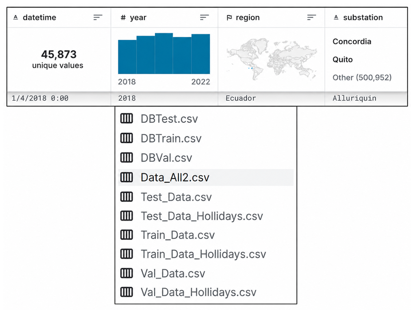
5.3. Dataset File Structure
As a result of the dataset construction process, an organized file structure was generated to facilitate its use in analysis and modeling processes.
The files Train_Data.csv, Val_Data.csv, and Test_Data.csv contain the numerical vectors corresponding to the 48 h temporal windows, which were previously normalized using min–max scaling applied per window. These files are organized in tabular format and can be directly used for training, validation, and evaluation of predictive models.
Additionally, the files DBTrain.csv, DBVal.csv, and DBTest.csv store metadata associated with each temporal vector, including feeder identification, start and end timestamps of each window, and the unique identifier of each record.
Furthermore, specific versions for non-working condition analysis were generated, corresponding to the files Train_Data_Holidays.csv, Val_Data_Holidays.csv, and Test_Data_Holidays.csv, which contain only filtered data for holidays and weekends.
Likewise, the file Data_All2.csv contains the complete set of preprocessed data before subset partitioning, allowing exploratory analysis or reconstruction of the data segmentation process.
This file organization facilitates data traceability, experiment reproducibility, and flexibility to apply different modeling approaches on the same dataset. The overall structure of the generated files is presented in Figure 9.
Figure 9.
Structure of generated dataset files, including training, validation, and test subsets, as well as specific versions for non-working days (holidays) and associated metadata files [26].
5.4. Future Applications of the Dataset
The dataset constructed in this study constitutes a structured foundation for the development and evaluation of electricity consumption forecasting models based on machine learning and deep learning techniques.
In this work, the primary focus is on the organization, documentation, and publication of the dataset, with the aim of providing a reproducible and well-structured data source for future research.
The proposed dataset enables the exploration of different modeling approaches for multi-horizon electricity demand forecasting, including traditional machine learning models, statistical methods, and advanced deep neural network architectures.
Additionally, the availability of this dataset facilitates the development of comparative studies between different forecasting methodologies, contributing to advances in research on smart electrical systems and energy demand analysis.
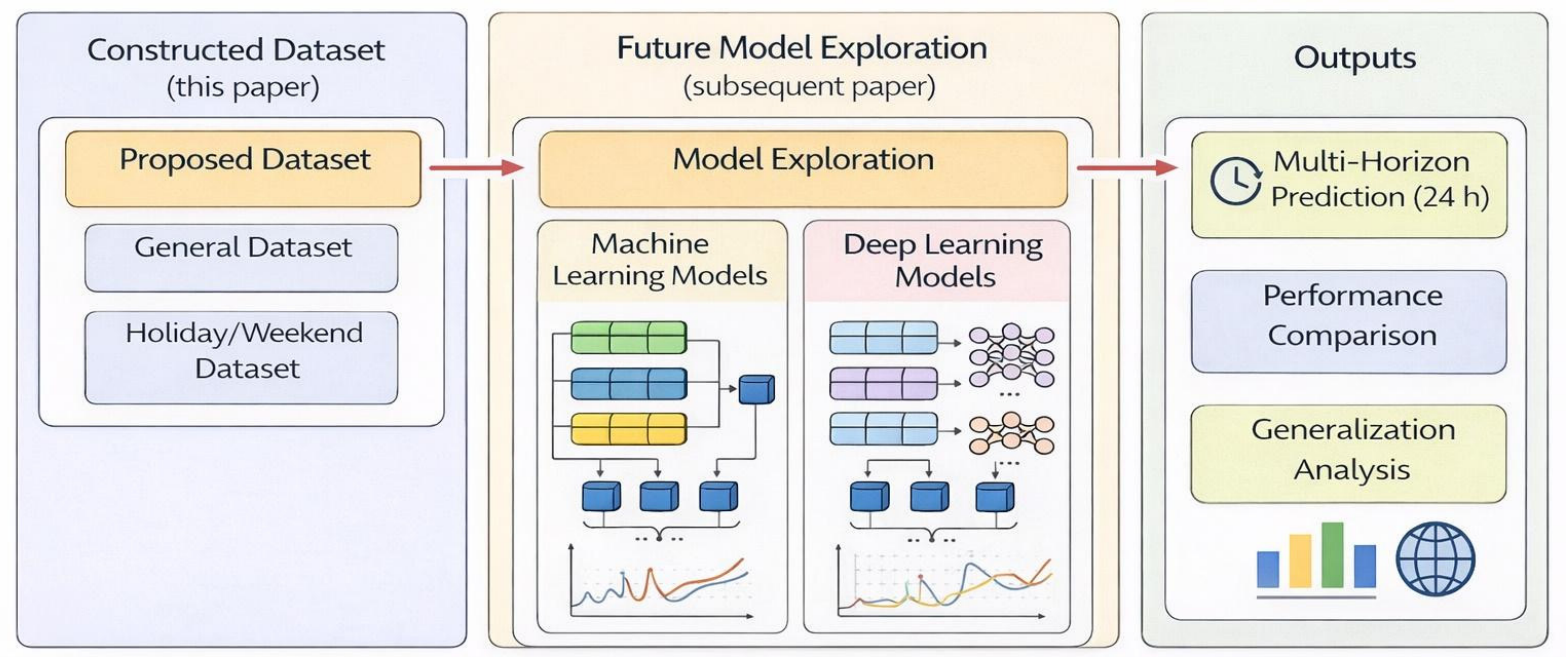
Figure 10 illustrates the conceptual framework for the potential use of the dataset in future research, from data preparation to predictive model training and performance evaluation.
Figure 10.
Conceptual framework for future exploration of predictive models using the proposed dataset, illustrating the transition from dataset construction to model training, prediction, and performance evaluation.
6. Availability, Reproducibility, and Ethical Considerations
6.1. Tools and Libraries Used
The processing, organization, and structuring of the data were implemented using widely adopted tools within the Python v3.10 scientific ecosystem, which enable the development of reproducible workflows for time series analysis and machine learning model training.
In particular, the following libraries were used:
- Pandas: This library was used for the manipulation and organization of tabular data, including file reading, management of temporal variables, and structuring of electricity consumption series. Pandas allowed chronological ordering of records by feeder and timestamp, as well as the generation of auxiliary variables required for labeling and segmenting the time series.
- NumPy: It was used to support efficient numerical operations and manipulation of multidimensional arrays. This library enabled basic statistical calculations, vector transformations, and operations required during the construction of 48 h temporal windows used in the dataset.
- Scikit-learn: It was used to implement the stratified data partitioning process. In particular, the StratifiedShuffleSplit method was applied, allowing the division of temporal vectors into training, validation, and test sets while preserving the distribution of electricity consumption levels across subsets.
The combined use of these tools enabled consistent and reproducible implementation of the methodological procedures described in previous sections, ensuring traceability of data cleaning, segmentation, and organization processes.
6.2. Ethical Considerations and Anonymization
This study was developed using operational data from real electrical system infrastructures. Consequently, strict confidentiality and anonymization criteria were applied to ensure responsible use of the information.
The data used correspond exclusively to aggregated measurements of electrical variables at the feeder level, such as apparent power, active power, and reactive power. These measurements reflect the overall behavior of the distribution system and do not contain information that allows identification of individual consumption habits or user-specific data.
Prior to processing, the data underwent an anonymization process involving the removal of sensitive identifiers related to electrical infrastructure. In particular, internal substation codes, specific operational references, and any information that could compromise system security were removed.
In this way, the published dataset maintains the scientific value required for research in electricity demand forecasting while preserving infrastructure confidentiality and complying with fundamental ethical principles related to responsible handling of technical information.
7. Descriptive Analysis of the Proposed Dataset
7.1. Descriptive Statistics
The first stage of the analysis consisted of examining the fundamental statistical properties of the dataset, including measures of central tendency and dispersion of electricity consumption recorded in the feeders.
The final dataset used in this study contains 882,570 hourly records, corresponding to the period from January 2018 to December 2022. These records come from multiple feeders within the Ecuadorian electrical distribution system and were obtained from real operational measurements recorded through SCADA infrastructure.
In particular, metrics such as mean, standard deviation, minimum and maximum values, as well as different percentiles of the electricity consumption distribution were calculated. These measures allow describing the range of variation of electricity demand and evaluating the presence of outliers in the time series.
Table 5 presents a summary of the main descriptive statistics of the variable kVA_tot, used as the main variable of the dataset.
Table 5.
Descriptive statistics of the variable kVA_tot.
The results show that electricity consumption presents considerable variability, reflected in the high observed standard deviation. This variability is associated with the diversity of consumption profiles across different feeders and with operational fluctuations in the electrical system over time.
Additionally, statistical consistency across dataset subsets was verified. The distributions corresponding to training, validation, and test sets were compared, showing similar statistical properties in terms of central tendency and dispersion. This confirms that the stratified partitioning procedure preserves the diversity of electricity consumption patterns.
7.2. Temporal Characteristics of Electricity Consumption
In addition to the global statistical analysis, the temporal characteristics of electricity consumption were examined in order to identify patterns associated with daily, annual, and contextual variations in demand.
The analysis of daily load profiles shows that electricity consumption presents characteristic variations throughout the day, with increases in demand mainly associated with periods of greater economic and social activity. These patterns reflect the typical behavior of electricity distribution systems, where demand usually increases during daytime and evening hours and decreases during the early morning.
Likewise, the temporal analysis makes it possible to identify variations across the different years included in the study period. These variations may be influenced by climatic factors, economic activity patterns, and changes in users’ consumption habits. In particular, the analyzed interval includes the period corresponding to the COVID-19 pandemic, which constitutes a relevant aspect of the dataset. During this period, mobility restrictions, the temporary reduction in certain commercial and industrial activities, and the increase in time spent at home may have modified the temporal distribution of electricity demand. Therefore, this interval may introduce atypical patterns that should be considered in subsequent studies involving the training, validation, and generalization of predictive models.
In equatorial regions such as Ecuador, although seasonal thermal variations are smaller than in temperate regions, there are climatic differences associated with rainy and dry seasons. These conditions may influence electricity consumption patterns through changes in temperature, humidity, productive activity, mobility, and the use of electrical equipment. In addition, the country’s geographical variability, including altitude differences among Andean, coastal, and tropical areas, may generate differentiated demand profiles even within the same equatorial region.
The identification of these temporal characteristics is fundamental for the development of predictive models capable of capturing the dynamics of electricity consumption at different temporal scales and under variable operational contexts. Likewise, these elements should be considered when using the dataset for studies on transfer learning across regions, model comparison, or generalization analysis in electrical systems with different climatic and socioeconomic conditions.
7.3. Comparison Between Working Days and Non-Working Days
To analyze potential differences in electricity consumption patterns under different operational conditions, a descriptive comparison was performed between the base dataset and the dataset corresponding to holidays and weekends.
The results show that consumption profiles for non-working days present different characteristics compared to those observed on working days. In particular, working days exhibit more pronounced demand peaks associated with commercial, industrial, and service activities.
In contrast, demand profiles for Sundays and holidays tend to present smoother load curves with lower variability throughout the day. This behavior reflects reduced economic activity and changes in consumption patterns associated with non-working conditions.
The comparison between both datasets allows identifying these structural differences in electricity demand behavior, which is especially relevant for developing predictive models capable of adapting to different operational contexts of the electrical system.
7.4. Illustrative Prediction Example
In order to demonstrate the applicability of the constructed dataset, an illustrative multi-horizon electricity consumption forecasting experiment was developed using a Long Short-Term Memory (LSTM) recurrent neural network model. This experiment is not intended to establish a definitive benchmarking among models, but rather to show that the structure of the dataset allows predictive models to be trained and evaluated using temporal input and output windows.
The model was trained using the base dataset, considering the previous 24 h of each temporal window as input and the following 24 h of the (kVA_tot) variable as output. Therefore, the forecasting strategy used corresponds to a 24 → 24 scheme, where the model receives a complete daily sequence and estimates the demand profile for the following day. The general configuration of the LSTM model was as follows:
- Model: General LSTM.
- Forecasting strategy: 24 input hours → 24 output hours.
- Architecture: 24:256:128:64:24.
- Trainable parameters: 512,280.
- Loss function: MAE.
- Optimizer: Adam.
- Learning rate: 0.0008.
- Batch size: 32.
- Maximum epochs: 500.
- Early stopping: patience = 12; min_delta = (1\times 10^{−4}).
- Framework: TensorFlow/Keras.
- Approximate training time: 65.3 h.
- Training samples: 730,778.
- Parameter/sample ratio: 0.7010.
- Parameter/input hour ratio: 21,345.
- Parameter/global value ratio: 0.0292.
The model performance was evaluated on the test set using global error metrics. The results obtained were as follows:
- Global MAPE: 4.123937%.
- Mean MAPE: 4.123899%.
- MAPE standard deviation: 5.305586.
- Median MAPE: 3.126412%.
- Minimum MAPE: 1.020097%.
- Maximum MAPE: 155.808378%.
- Global MAE: 62.986224.
- Global RMSE: 112.008865.
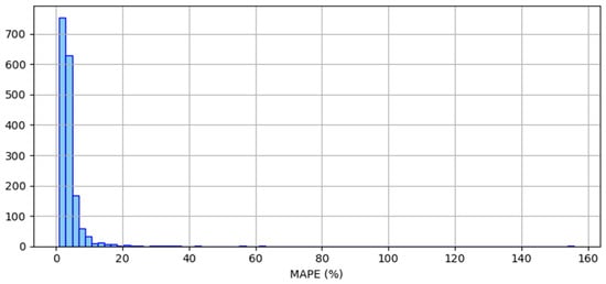
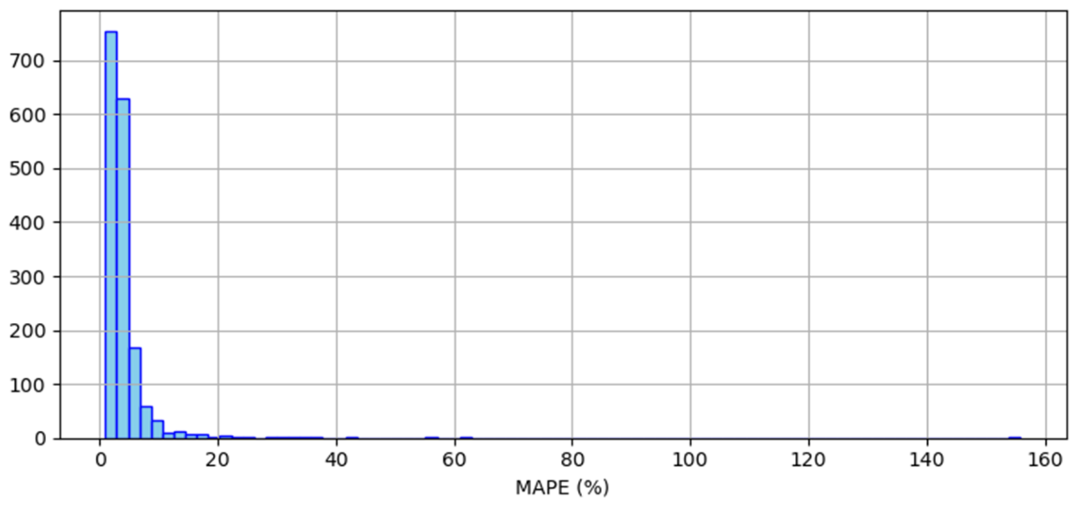
The results show that the LSTM model achieves a global MAPE of 4.12%, which indicates that the dataset contains sufficient temporal information to capture relevant patterns in electricity demand. Likewise, the median MAPE, equivalent to 3.13%, indicates that most predictions present relatively low errors. However, the maximum MAPE value reveals the existence of some atypical cases with high errors, possibly associated with abrupt load variations or non-recurring operational conditions.
As a first approximation to the model’s performance, the global distribution of the mean absolute percentage error was examined. Figure 11 presents the histogram of the MAPE values obtained for the evaluated vectors, making it possible to observe the main concentration of errors in low ranges and the presence of some isolated cases with higher errors.
Figure 11.
Histogram of the MAPE error distribution (%) obtained in the evaluation of the LSTM model on the general dataset.
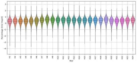
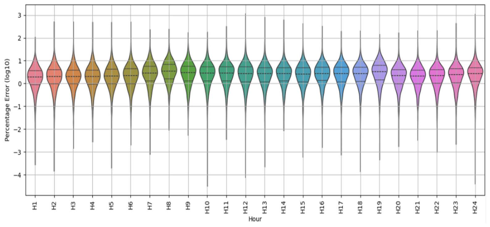
In order to further analyze the behavior of the error, its distribution along the 24 h forecasting horizon was examined. For this purpose, the error was calculated for each of the output hours and its distribution was represented using a violin plot. Figure 12 shows the distribution of the error expressed as (\log_{10}(MAPE)) for each hour of the output horizon, making it possible to identify error dispersion and evaluate whether there are hours with greater predictive variability.
Figure 12.
Distribution of the hourly prediction error expressed as (\log_{10}(MAPE)) for the 24 h of the LSTM model output horizon.
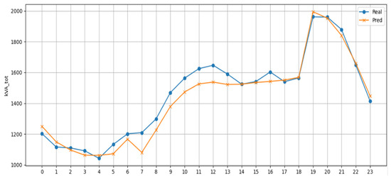
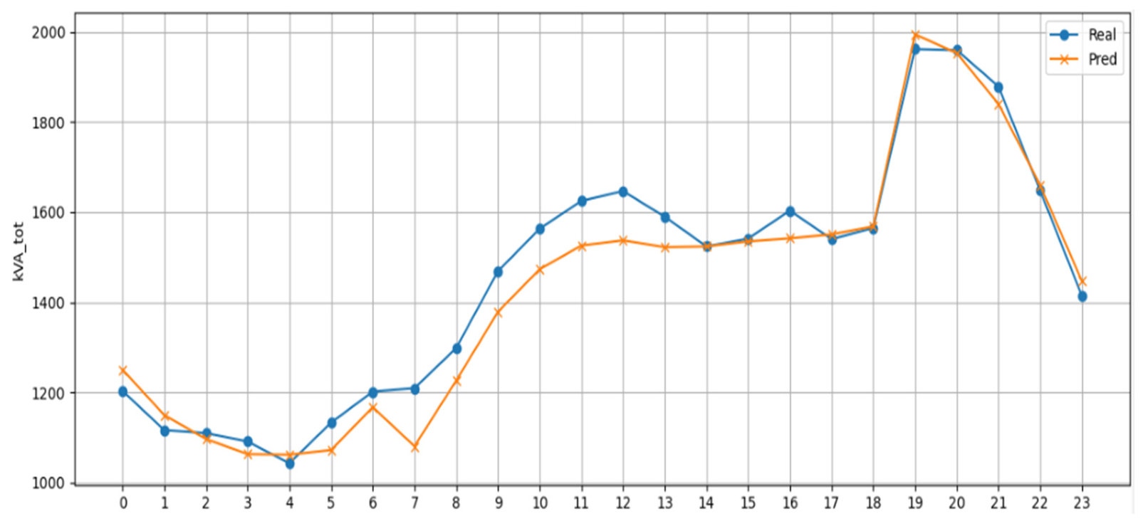
Finally, to directly illustrate the predictive behavior of the model on a specific sequence, a representative comparison example between measured and estimated values is presented. Figure 13 shows a 24 h prediction case for a representative feeder, where it can be observed that the model adequately reproduces the general trend of electricity consumption, including the approximate location of peaks and valleys in the daily load profile.
Figure 13.
Measured vs. forecasted 24 h (kVA_tot) profile using the LSTM model for a representative feeder (multi-step forecasting example).
These results show that the proposed dataset constitutes a suitable basis for the development and evaluation of multi-horizon electricity consumption forecasting models. However, this experiment should be interpreted as an initial demonstration of applicability. A comprehensive comparison against baseline models, such as persistence, ARIMA, SVR, or other Deep Learning architectures, will be necessary in future work to establish a complete benchmarking framework.
7.5. Evaluation Metrics
To evaluate the performance of the predictive model, three metrics widely used in time series forecasting problems were applied: MAPE, MAE, and RMSE. The mean absolute percentage error (MAPE) is defined as:
where represents the actual value, the predicted value, and (n) the total number of observations evaluated.
The mean absolute error (MAE) is calculated as:
The root mean square error (RMSE) is defined as:
These metrics make it possible to evaluate the model’s performance from different perspectives. MAPE expresses the error in percentage terms, MAE measures the average magnitude of the error in the real units of the analyzed variable, and RMSE penalizes large errors more strongly.
8. Conclusions
This work presented a structured review of public datasets used in research on electricity consumption forecasting, along with the description and publication of a new electricity demand dataset from an equatorial region.
The review made it possible to identify that many of the datasets widely used in the literature are concentrated in Europe and North America and are mainly oriented toward residential, appliance-level, or individual customer measurements. This characteristic limits their direct applicability in studies focused on electricity distribution networks, where aggregated data at the feeder or substation level are required.
As the main contribution, this study documented a dataset constructed from real measurements obtained from electrical substations in Ecuador during the 2018–2022 period. The dataset was standardized to a temporal resolution of 1 h and organized through 48 h temporal windows, composed of 24 input hours and 24 output hours, which enables its use in multi-horizon electricity demand forecasting tasks.
The dataset was structured into training, validation, and test subsets, generated through a stratified partition based on the mean value of the (kVA_tot) variable during the 24 input hours. This strategy made it possible to preserve a balanced distribution of demand levels across the different subsets and improve the consistency of the predictive experiments.
The descriptive analysis showed that the dataset contains 882,570 hourly records and captures significant variability in electricity consumption, associated with differences among feeders, daily patterns, working- and non-working-day conditions, and relevant temporal changes, including the period of the COVID-19 pandemic. In addition, the illustrative experiment using an LSTM model demonstrated the applicability of the dataset for multi-horizon forecasting tasks, achieving a global MAPE of 4.12%, a global MAE of 62.99, and a global RMSE of 112.01.
Despite these contributions, the dataset presents some limitations. First, it corresponds to a specific geographical region; therefore, its direct transfer to other electrical systems should be carried out with caution. Equatorial climatic conditions, the altitude of the analyzed areas, the structure of the distribution network, and local consumption patterns may influence the generalization of models trained with these data.
Likewise, the dataset does not incorporate external variables such as temperature, precipitation, humidity, solar radiation, socioeconomic information, or detailed holiday attributes. The future inclusion of these variables would allow the development of more robust models, the evaluation of domain adaptation strategies, and the improvement of the transferability of predictive models to other climatic or operational regions.
Finally, the publication of this dataset is expected to contribute to expanding the geographical diversity of data available for research in energy systems and to facilitate the development of comparative studies aimed at improving electricity demand forecasting in distribution networks located in equatorial regions.
Author Contributions
Conceptualization, E.F.M.-G. and D.B.; methodology, E.F.M.-G.; software, E.F.M.-G.; validation, E.F.M.-G., D.B. and M.P.C.; formal analysis, E.F.M.-G.; investigation, E.F.M.-G.; resources, D.B. and M.P.C.; data curation, E.F.M.-G.; writing—original draft preparation, E.F.M.-G.; writing—review and editing, D.B. and M.P.C.; visualization, E.F.M.-G.; supervision, D.B. and M.P.C.; project administration, E.F.M.-G.; funding acquisition, N/A. All authors have read and agreed to the published version of the manuscript.
Funding
This research received no external funding.
Data Availability Statement
The original contributions presented in this study are included in the article. Further inquiries can be directed to the corresponding author.
Conflicts of Interest
The authors declare no conflict of interest.
References
- Salas, J.; Maldonado, J.; Llerena, V. Evolución Del Consumo y Generación de Energía Eléctrica en Ecuador: Análisis del Balance Energético y Diversificación de la Matriz Energética (2021–2024). Talentos Revista de Investigación. 2025. Available online: https://doi.org/10.33789/talentos.12.1.204 (accessed on 10 January 2026). [CrossRef] [Scilit]
- Li, W.; Li, T. Comparison of deep learning models for predictive maintenance in industrial manufacturing systems using sensor data. Sci. Rep. 2025, 15, 23545. [Google Scholar] [CrossRef] [Scilit] [PubMed]
- Hu, H.; Gong, S.; Taheri, B. Energy demand forecasting using convolutional neural network and modified war strategy optimization algorithm. Heliyon 2024, 10, e27353. [Google Scholar] [CrossRef] [Scilit] [PubMed]
- Ragupathi, C.; Dhanasekaran, S.; Vijayalakshmi, N.; Salau, A.O. Prediction of electricity consumption using an innovative deep energy predictor model for enhanced accuracy and efficiency. Energy Rep. 2024, 12, 5320–5333. [Google Scholar] [CrossRef] [Scilit]
- Akhtar, S.; Adeel, M.; Iqbal, M.; Namoun, A.; Tufail, A.; Kim, K.-H. Deep learning methods utilization in electric power systems. Energy Rep. 2023, 10, 2138–2151. [Google Scholar] [CrossRef] [Scilit]
- Kelly, J.; Knottenbelt, W. The UK-DALE dataset, domestic appliance-level electricity demand and whole-house demand from five UK homes. Sci. Data 2015, 2, 150007. [Google Scholar] [PubMed]
- Kolter, J.; Johnson, M. A Public Data Set for Energy Disaggregation Research. 2011. Available online: https://www.semanticscholar.org/paper/REDD-%3A-A-Public-Data-Set-for-Energy-Disaggregation-Kolter-Johnson/db3ea129add716192f11d41e605c0020ee2488d7 (accessed on 15 January 2026).
- Murray, D.; Stankovic, L. An electrical load measurements dataset of United Kingdom households from a two-year longitudinal study. Sci. Data 2017, 4, 160122. [Google Scholar] [CrossRef] [Scilit] [PubMed]
- Makonin, S.; Ellert, B.; Bajic, I.; Popowich, F. Electricity, water, and natural gas consumption of a residential house in Canada from 2012 to 2014. Sci. Data 2016, 3, 160037. [Google Scholar] [CrossRef] [Scilit] [PubMed]
- Ginzburg, E.; Lifshits, P.; Machlev, R.; Belikov, J.; Krieger, Z.; Levron, Y. Technical Challenges of AI Data Center Integration into Power Grids—A Survey. Energies 2025, 19, 137. [Google Scholar] [CrossRef] [Scilit]
- Quesada, C.; Astigarraga, L.; Merveille, C.; Borges, C.E. An electricity smart meter dataset of Spanish households: Insights into consumption patterns. Sci. Data 2024, 11, 59. [Google Scholar] [CrossRef] [Scilit] [PubMed]
- Ramos Alvarado, E.J.; Llerena Guevara, R.M.; Flowers Jaen, M.Q.; Rivas Pinargote, B.A.; Cornejo Mantuano, J.A. La importancia del consumo energético en el desarrollo económico de Ecuador. LATAM Lat. Am. J. Soc. Sci. Humanit. 2025, 6, 877–892. [Google Scholar] [CrossRef] [Scilit]
- Banad, Y.M.; Sharif, S.S.; Rezaei, Z. Artificial intelligence and machine learning for smart grids: From foundational paradigms to emerging technologies with digital twin and large language model-driven intelligence. Energy Convers. Manag. X 2025, 28, 101329. [Google Scholar] [CrossRef] [Scilit]
- Defaz, V.; Ortiz, L. Predicción de Consumo de Energía Eléctrica en Hogares Utilizando Modelos de Aprendizaje Automático. 2025. Available online: https://repositorio.uide.edu.ec/bitstream/37000/8546/1/UIDE-Q-TCDM-2025-21.pdf (accessed on 2 February 2026).
- Sivarajah, U.; Mustafa, M.; Irani, Z.; Weerakkody, V. Critical analysis of Big Data challenges and analytical methods. J. Bus. Res. 2017, 70, 263–286. [Google Scholar] [CrossRef] [Scilit]
- Laurencio, R.M.; Breff, O.T.; Ramirez, S.M.; Jiménez, J.D. Predicción de Consumo y Demanda de Electricidad Mediante Redes Neuronales Artificiales y Algoritmo Iterativo. Rev. Politécnica 2024, 54, 3. [Google Scholar] [CrossRef] [Scilit]
- Godahewa, R.; Bergmeir, C. Electricity Hourly Dataset. 2020. Available online: https://zenodo.org/records/4656140 (accessed on 25 January 2026).
- Sierra, D.; Petro, J.; Ruiz, D. Machine learning models for predicting geomagnetic storms across five solar cycles using Dst index and heliospheric variables. Adv. Space Res. 2024, 74, 3483–3495. [Google Scholar] [CrossRef] [Scilit]
- Pecan Street. Consumo Energético y Generación Solar. 2023. Available online: https://www.pecanstreet.org/dataport/explore/ (accessed on 1 February 2026).
- Trindade, A. ElectricityLoadDiagrams20112014. 2015. Available online: https://archive.ics.uci.edu/ml/datasets/ElectricityLoadDiagrams20112014 (accessed on 26 January 2026).
- Truong, D.; Chou, J. Scientific approach to problem solving-inspired optimization of stacking ensemble learning for enhanced civil engineering informatics. Artif. Intell. Rev. 2025, 58, 404. [Google Scholar] [CrossRef] [Scilit]
- Altamimi, E.; Al-Ali, A.; Malluhi, Q.M.; Al-Ali, A.K. Smart grid public datasets: Characteristics and associated applications. IET Smart Grid 2024, 7, 503–530. [Google Scholar] [CrossRef] [Scilit]
- Molina, J.; Quezada, D. Análisis Operativo-Comercial de la Implementación del Sistema SCADA/OMS-MWM/DMS en Subestaciones y Redes de Distribución de la Empresa Eléctrica Azogues. Energia 2024, 11, 162–168. [Google Scholar]
- Romero, R.E.; Carmona, D.R.; Wagner, D.M.; Carillo, S.; Rojo, J.L. Sistemas avanzados de gestión de la distribución (ADMS). Ind. Econ. 2024, 431, 131–144. [Google Scholar]
- AVENSYS. Estructura de Relés de Protección Digital. 2020. Available online: http://www.avensys.co.kr/463565164853560-4837254840442285120444592-4439651312.html (accessed on 30 January 2026).
- Méndez, E.F. Electrical Power Data Equatorial Regions (Ecuador). 2026. Available online: https://www.kaggle.com/datasets/erikfmndez/electrical-power-data-equatorial-regions-ecuador (accessed on 1 April 2026).

Disclaimer/Publisher’s Note: The statements, opinions and data contained in all publications are solely those of the individual author(s) and contributor(s) and not of MDPI and/or the editor(s). MDPI and/or the editor(s) disclaim responsibility for any injury to people or property resulting from any ideas, methods, instructions or products referred to in the content. |
© 2026 by the authors. Licensee MDPI, Basel, Switzerland. This article is an open access article distributed under the terms and conditions of the Creative Commons Attribution (CC BY) license.