Power Path Dynamic Reconfiguration Method for Integrated Energy Storage-Soft Open Point

Abstract

Conventional soft open points (SOPs) suffer from limited transfer capacity during distribution network faults. To address this issue, this paper proposes an integrated energy storage system and soft open point (ES-SOP) along with a power path dynamic reconfiguration method. The device consists of an M × N AC switch matrix, N AC/DC converters, and a common DC bus with energy storage. This structure provides three distinct power paths: a mechanical direct path, a third-party grid path, and an energy storage path. A seamless reconfiguration technology is developed to eliminate inrush currents during mechanical switching. It combines multi-unit virtual synchronous generator (VSG) pre-synchronization with a DC bus voltage droop coordination mechanism. The overall control follows a two-time-scale strategy. On a long time scale, a heuristic rule selects the most suitable healthy grid as the mechanical source. On a short time scale, the droop parameters of the converters are optimized to autonomously share the remaining power between the third-party grid path and the energy storage path. This allocation minimizes losses and requires no fast communication. Hardware-in-the-loop experiments verify the performance: the proposed method completely suppresses inrush current, keeps DC bus voltage fluctuation below 20 V during mode transitions, and achieves a transfer efficiency of approximately 98.5%.

1. Introduction

In recent years, with the widespread integration of distributed generation and electric vehicles, the operation scenarios of distribution networks have become increasingly complex. Traditional distribution networks are mostly radial, with feeder interconnections via normally open points (NOPs), and rely on mechanical switches for power transfer during faults. However, mechanical switches operate slowly and cause large inrush currents, making it difficult to meet the supply continuity requirements of sensitive loads [1].

The soft open point (SOP) is a power electronic device based on back-to-back converters. It replaces conventional normally open points (NOPs) to enable flexible feeder interconnection [1]. SOPs can regulate active and reactive power rapidly and continuously, which helps to optimize power flow. During a grid fault, an SOP can quickly switch to voltage source mode. This supports the off-grid side voltage and frequency and allows for seamless load transfer [2,3,4]. In recent years, multi-terminal SOPs and energy storage-integrated SOPs (ES-SOPs) have further expanded the regulation capability of these systems [5,6]. Efficient coordination between energy storage and multiple power sources is essential for resilient and autonomous operation, as highlighted in a recent overview of self-sufficient energy-harvesting devices [7]. Academic research on SOPs covers many aspects, including topologies [8,9,10], control strategies [11,12,13], optimal scheduling [14,15,16,17], and reliability assessment [18].

Fault transfer control of SOPs can be divided into two main categories. The first category is mode-switching control. In normal conditions, the SOP operates in grid-following mode; after a fault, it switches to grid-forming mode to support the off-grid voltage [19]. This approach enables fast voltage support, but the mode transition itself can cause voltage and current transients. It also relies on fast communication and precise synchronization. Pre-synchronization control and virtual synchronous generator (VSG) methods have been proposed to make the switching smoother [20]. These improvements reduce transients, yet they still operate within a purely power-electronic path. All the transferred power must pass through AC-DC-AC converters, which leads to conversion losses and limits the transfer capacity to the converter rating.

The second category is the hybrid soft open point (HSOP), which places a mechanical switch in parallel with the SOP [21]. During normal operation, the SOP manages the power flow. After a fault, the mechanical switch closes and provides a low-loss bypass for the load current. This reduces long-term operating losses compared with a pure SOP. However, the mechanical switch in an HSOP connects to a fixed healthy grid. It cannot select the most suitable source based on real-time spare capacity. Moreover, when the mechanical switch closes, a phase difference between the two sides can cause a large inrush current, which threatens equipment safety [21].

More recently, multi-port SOPs have drawn attention to the combination of an AC switch matrix and multiple power converters. Using the switch matrix, several converters can connect flexibly to different grids and share a common DC bus with energy storage. This structure can, in principle, provide multiple power paths: a low-loss mechanical direct path, a third-party grid path via AC-DC-AC conversion, and an energy storage path. The core challenge is how to dynamically reconfigure these paths and optimally allocate power according to grid capacity, storage state, and load demand while keeping the switching process smooth and safe. Existing studies on path reconfiguration and power allocation have two main limitations. First, they tend to treat mechanical and power-electronic paths separately without coordinating them. Second, their power allocation methods usually rely on centralized optimization and heavy communication, which is difficult to realize in distribution networks with limited measurements [22,23].

Furthermore, the strong volatility of renewable generation and load forecast errors challenges the robustness of SOP operation. Deterministic optimization cannot guarantee voltage security. Stochastic programming needs accurate probability distributions, which are hard to obtain in practice [5]. Robust optimization [4,15] and model predictive control [14] have been applied to SOP scheduling under uncertainty. Yet these methods still depend on global system models and high-speed communication, which are not always available in actual distribution networks.

To address the above problems, this paper proposes a power path dynamic reconfiguration method for ES-SOP. The device consists of an M × N AC switch matrix, N AC-DC converters, and a common DC bus with energy storage access. The main contributions of this paper are as follows: (1) First, the seamless technology for power path reconfiguration is elaborated in detail, including a multi-unit virtual synchronous generator (VSG) pre-synchronization method and a DC bus voltage droop coordination mechanism. (2) A two-time-scale power path dynamic reconfiguration strategy is proposed. On the long time scale, the mechanical direct path is optimized based on the long-term available capacity of each grid. On the short time scale, automatic power allocation between the third-party grid path and the energy storage path is achieved by optimizing the DC voltage droop parameters. The rest of the paper is organized as follows: Section 2 introduces the system topology and definitions of the three power paths, Section 3 elaborates the seamless reconfiguration technology, Section 4 presents the two-time-scale power path dynamic allocation strategy, Section 5 verifies the proposed method through simulations, and Section 6 concludes the paper.

2. Proposed Methodology

2.1. System Topology Definition

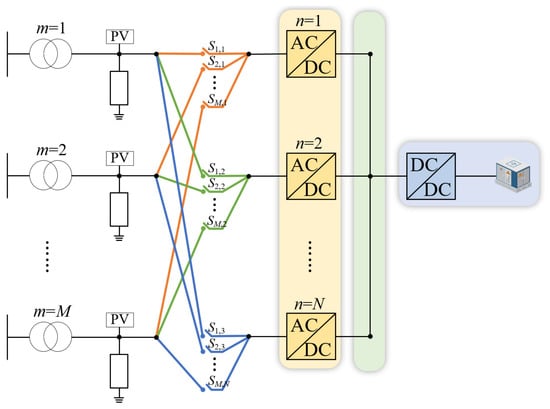
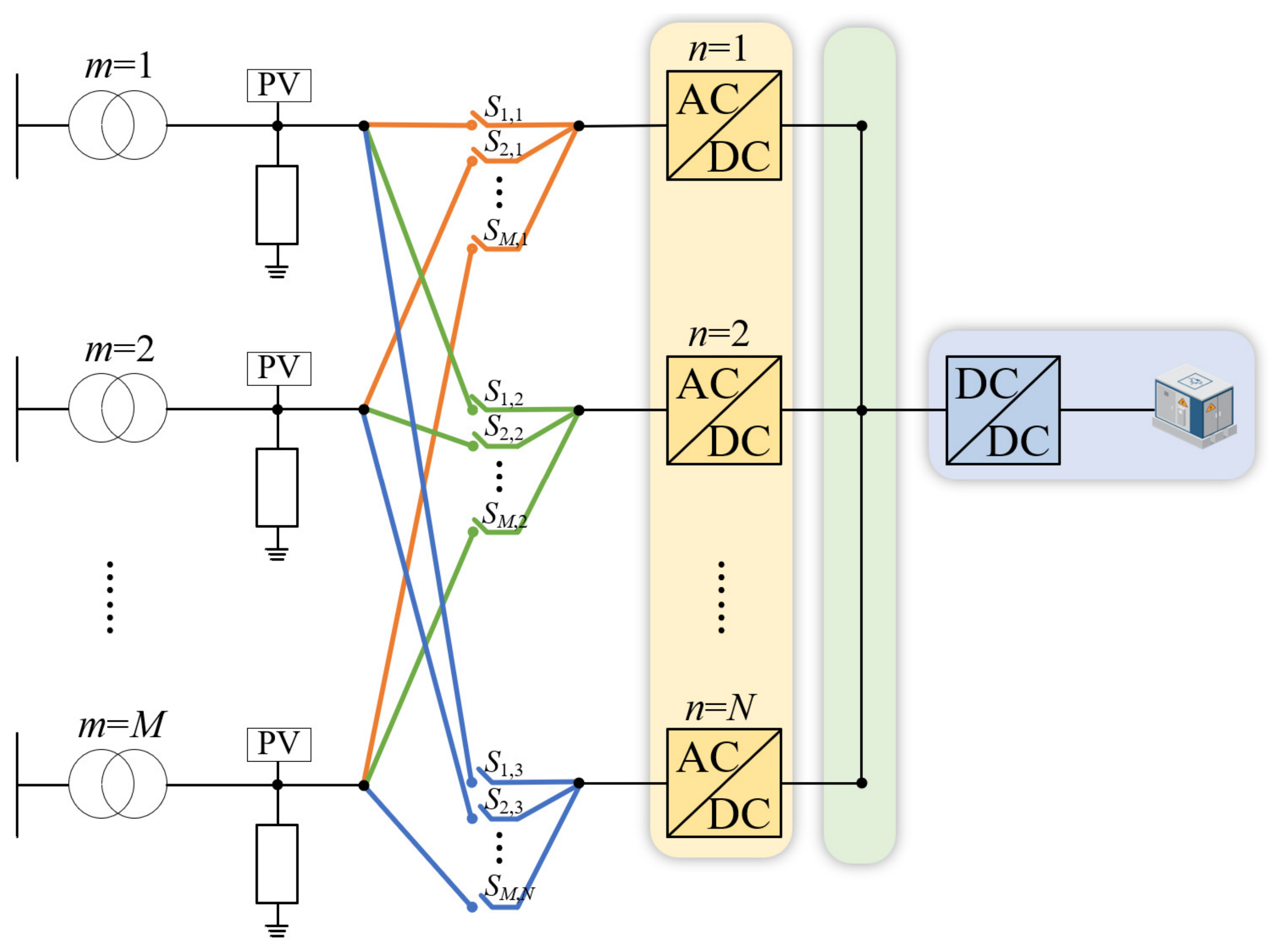
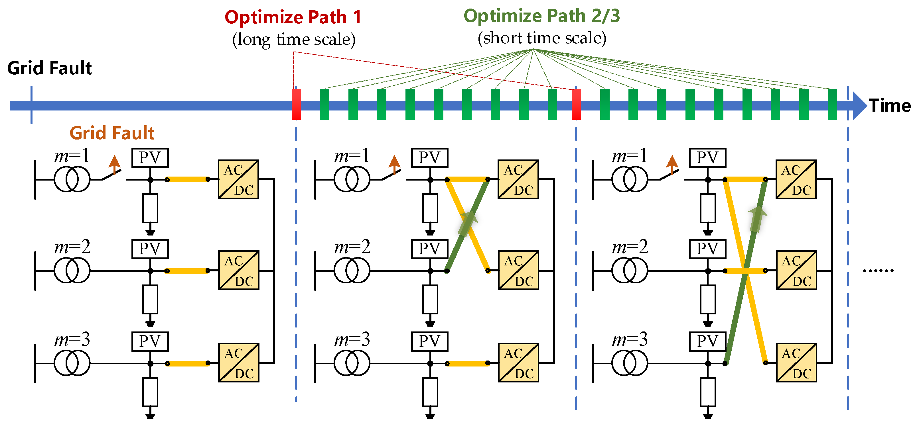
As shown in Figure 1, the device has M AC interfaces (numbered m = 1, …, M) connecting to M distribution grids and N AC-DC converters (numbered n = 1, …, N) whose DC sides are connected in parallel to a common DC bus. The DC bus can be connected to energy storage systems. The AC side of each converter is connected to the AC interface m via a controllable switch S_m,n, forming an M × N AC switch matrix:

$$S(t)=\left[\begin{array}{cccc}{S}_{1,1}(t)& S_{1,2}(t)& \cdots & S_{1,N}(t)\\ S_{2,1}(t)& S_{2,2}(t)& \cdots & S_{2,M}(t)\\ ⋮& ⋮& \ddots & ⋮\\ S_{M,1}(t)& S_{N,2}(t)& \cdots & S_{M,N}(t)\end{array}\right]$$

(1)

where matrix elements of S_m,n = 0 and S_m,n = 1 represent the OFF and ON states of the corresponding mechanical switches, respectively.

Figure 1. The structure of ES-SOPs with an AC switch matrix.

2.2. The Basic Operation Principles

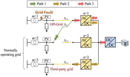
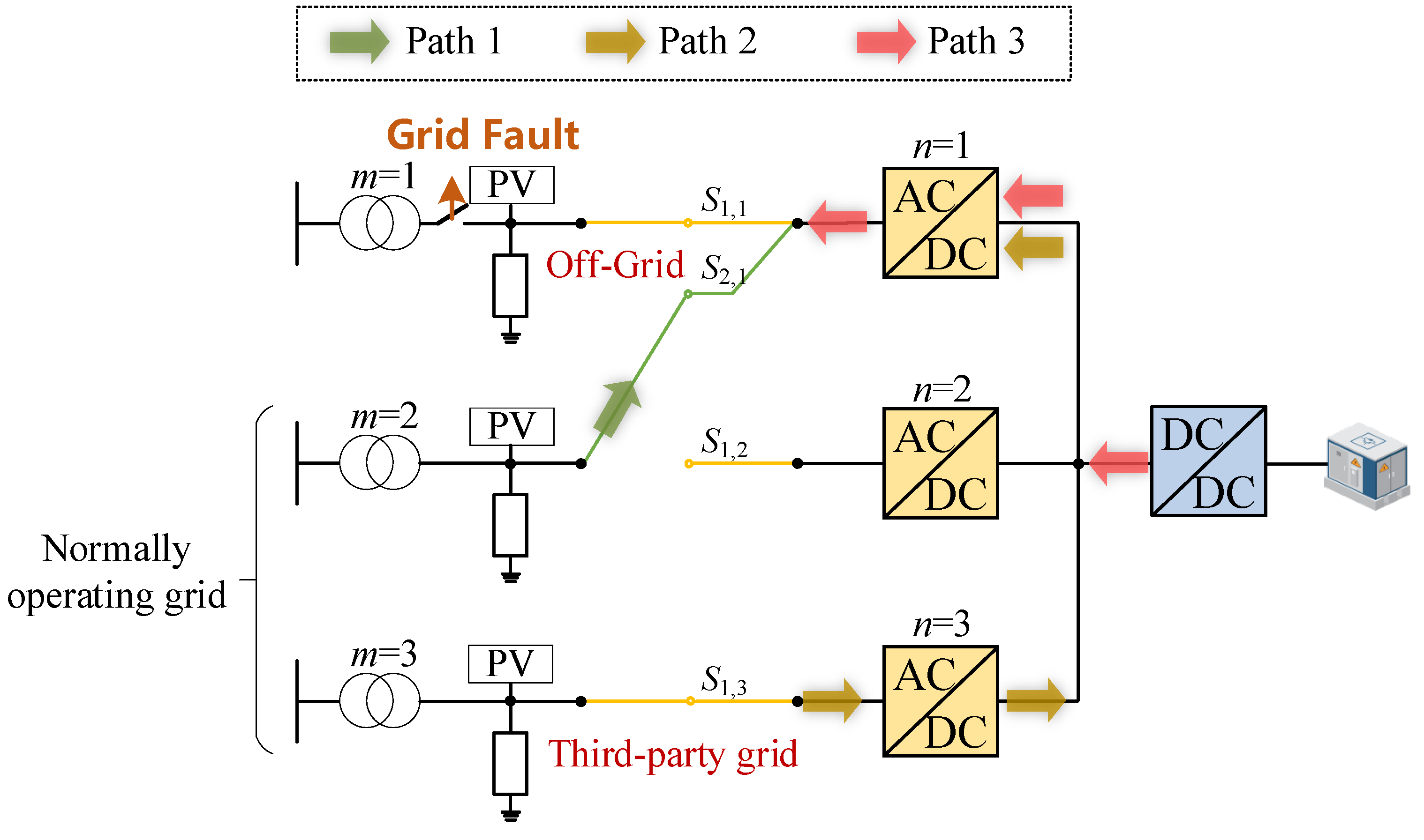
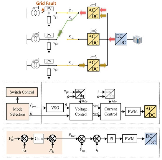
Taking grid 1 as an off-grid example, its load $P_{\mathrm{load}}$ can be supplied by the following paths shown in Figure 2. The details of the three paths are given below:

Figure 2. Illustration of three power paths.

Path 1: Mechanical direct path. Select a normally operating grid $m$ ($m\ge 2$). Then, close the mechanical switch S_1,1. Doing so, the power flows directly from grid $m$ to grid 1. The loss is negligible. But it is limited by the maximum power that the grid $m$ can provide, which is defined as $P_{m,\mathrm{line},\max }$.

Path 2: Third-party grid path. Any normally operating grid $m$ can inject power into the DC bus via an AC-DC converter and then be inverted to the off-grid side via a DC-AC converter. This path needs two stages of AC-DC conversion, with total efficiency ${\eta }_{\mathrm{acdc}}\approx 0.94\sim 0.96$ and loss coefficient ${\alpha }_{\mathrm{acdc}}=1/{\eta }_{\mathrm{acdc}}-1\approx 0.04\sim 0.06$. But it is flexible in capacity and can be multi-source coordinated.

Path 3: Energy storage path. Energy storage is boosted by a DC-DC converter to the DC bus and then inverted to the off-grid side. This path undergoes DC-DC and DC-AC two-stage conversion, with total efficiency ${\eta }_{\mathrm{ess}}\approx 0.93\sim 0.95$ and loss coefficient ${\alpha }_{\mathrm{ess}}=1/{\eta }_{\mathrm{ess}}-1\approx 0.05\sim 0.07$, and is limited by the SOC of the energy storage.

The energy of Path 2 and Path 3 first converges to the common DC bus and is then inverted to AC by the AC/DC converter. Thus, the converter acts as a controllable load on the DC bus, and the power it absorbs $P_{\mathrm{inv}}$ equals $P_{\mathrm{load}}$ minus the Path 1 power.

During path switching, two types of transients must be considered and eliminated. Firstly, when the mechanical switch of Path 1 is closed, a voltage phase difference between the two sides may cause a large current. Secondly, when a DC/AC converter changes its operation modes, the DC bus voltage may fluctuate. To address these issues, the proposed method employs a seamless reconfiguration technology detailed in Section 3, which includes multi-unit VSG pre-synchronization and a DC bus voltage droop coordination mechanism.

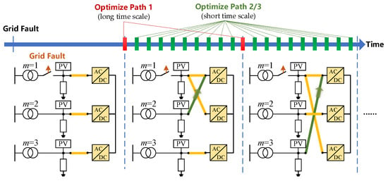
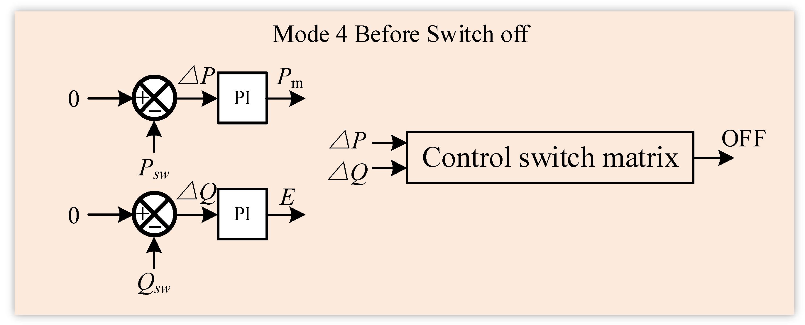
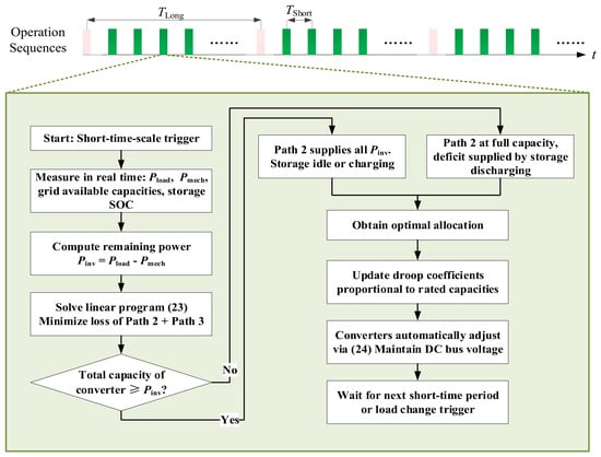
From an operational perspective, the method contains a two-time-scale optimization, as illustrated in Figure 3. On the long time scale of about one hour, the source grid for Path 1 is optimally chosen based on the long-term available capacities of each normally operating grid, thereby avoiding frequent mechanical operations. On the short time scale of seconds to minutes, after the mechanical path is fixed, the remaining load is automatically allocated between Path 2 and Path 3 by tuning the DC voltage droop parameters. This allocation minimizes total losses and can even charge the storage when surplus power is available. The detailed two-time-scale dynamic allocation strategy is presented in Section 4.

Figure 3. Brief illustration of two-time-scale optimization.

The key scientific contributions that distinguish this work from existing SOP variants are summarized in Table 1 and elaborated below.

Table 1. Comparison of the proposed method with existing SOP technologies (✓ Availability; ✗ Unavailability).

Feature	Traditional SOP	HSOP	Multi-Terminal SOP	Existing ES-SOP	This Work
Hybrid path coordination (mechanical + converter + storage)	✗	✓	✗	✗	✓
Energy storage integration and optimization	✗	✗	✗	✓	✓
Seamless mechanical switching	✗	✗	✗	✗	✓
Local droop-based allocation without communication	✗	✗	✗	✗	✓
HIL validation	✓	✓	✓	✓	✓

A traditional SOP uses only power electronic converters. It has no mechanical path and no storage. All transferred power must go through AC-DC-AC conversion. This causes high losses. The transfer capacity is limited by the converter rating. Power allocation usually needs central control or fast communication.

An HSOP adds a mechanical bypass switch to an SOP. After the switch closes, the load can flow through a low-loss path. But the mechanical path is fixed to one grid. It cannot choose the best source. Closing the switch can also cause a large inrush current. There is no storage to help. Power sharing still depends on communication.

Multi-terminal SOPs connect several converters on a common DC bus. They can move power between multiple feeders. But every path is still power electronic. There is no mechanical bypass and no storage. Control is usually centralized and needs communication.

Existing ES-SOPs put a battery on the DC bus of an SOP. The storage is mainly used for steady-state tasks, like peak shaving or smoothing. It is not actively coordinated with path switching during a fault. There is no mechanical direct path. Conversion losses still exist. Power scheduling usually relies on communication.

The proposed system uses three paths together: a mechanical direct path, a converter path, and a storage path. The mechanical path carries the base load with almost no loss. A dedicated control method lets the mechanical switch close without inrush current. Power sharing between the converter and storage paths happens automatically.

The proposed ES-SOP reduces operational losses by utilizing the loss-free mechanical direct path, eliminates outage costs through seamless transfer without inrush currents, and defers network upgrades by flexibly coordinating power paths during contingencies. It also extends equipment life and avoids expensive communication infrastructure. Overall, the method yields substantial long-term savings with a favorable payback on the incremental hardware investment.

3. Seamless Reconfiguration Technology for Power Path Switching

During the reconfiguration of power paths, the AC/DC converters connected to the off-grid side must switch among several control modes to enable smooth connection of Path 1. Two critical moments require special attention. When closing the mechanical switch to establish Path 1, a voltage phase difference between the two sides may cause an inrush current. When opening the mechanical switch to change the source grid, power must be reduced to zero before opening to avoid arcing and transients.

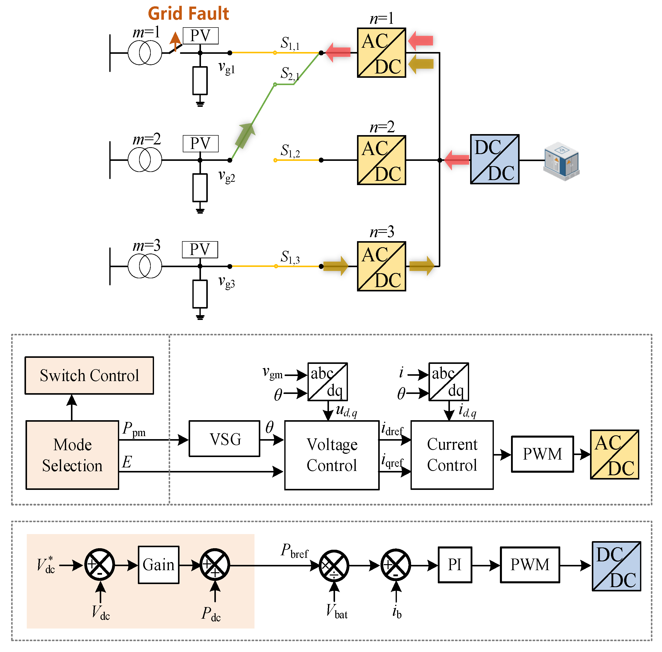
To address the above challenges, the converter adopts a hierarchical control architecture, as shown in Figure 4. The outer layer is the mode selection layer, which generates two key parameters: the mechanical power command P_pm and the internal voltage amplitude command $E$. These parameters are then sent to the VSG control layer, which emulates the swing equation of a synchronous machine to produce the output angle $\theta$ and also passes the amplitude command. Finally, the voltage and current control layer regulates the converter’s output voltage and current to track these references. The VSG layer, voltage layer, and current layer are shared across all operation modes, where only the outer layer changes its behavior depending on the mode.

Figure 4. Block diagrams of power path reconfiguration.

Based on this architecture, the converter is designed to operate in four distinct control modes, as summarized in Table 2. In each mode, the outer layer produces $P_m$ and $E$ in a different way, while the inner layers remain unchanged. This design ensures seamless transitions because only the reference generation logic is switched, and the inner loops continue to run without reconfiguration. The following subsections detail each control mode.

Table 2. Four control modes of the AC/DC converter.

Mode	Name	How Ppm and E Are Determined
1	Grid-connected mode	DC voltage droop gives Ppm; E from reactive power command
2	Off-grid mode	Frequency droop gives Ppm; reactive droop gives E
3	Pre-synchronization mode	Phase PI adds to frequency droop; amplitude PI adds to reactive droop
4	Power transfer mode	Closed-loop PI control drives mechanical switch power to zero

3.1. Mode 1: Grid-Connected Operation with DC Voltage Droop Control (Grid-Connected Mode)

When the mechanical switch is closed and Path 1 is active, the off-grid side is electrically connected to a normally operating grid. In this situation, the converter operates in grid-connected mode. Its primary function is to exchange power with the grid while participating in the regulation of the common DC bus voltage.

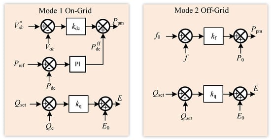
The block diagrams of this mode are given in Figure 5. In this mode, the outer layer determines the mechanical power command $P_{pm}$ via a DC voltage droop controller. The control law is

$$P_{pm}=P_{\mathrm{dc}}^{\mathrm{ff}}-k_{\mathrm{dc}}(V_{\mathrm{dc}}^{*}-V_{\mathrm{dc}}),$$

(2)

where $P_{\mathrm{dc}}^{\mathrm{ff}}$ is a feedforward power derived from the short-time-scale optimization, $k_{\mathrm{dc}}$ is the droop coefficient, and $V_{\mathrm{dc}}^{*}$ is the reference DC voltage. The internal voltage amplitude $E$ is set according to a reactive power command, typically to maintain a specified power factor or to support the local voltage. The resulting $P_{pm}$ and $E$ are then sent to the shared VSG layer.

Figure 5. Block diagrams of Mode 1 and Mode 2.

When the mechanical switch is closed and Path 1 is active, the off-grid side is electrically reconnected to a healthy grid. In this situation, the converter operates in grid-connected mode. Its primary functions are to exchange active and reactive power with the grid and to participate in the regulation of the common DC bus voltage.

In this mode, the outer control layer determines the mechanical power command $P_{\mathrm{p}\mathrm{m}}$ through a DC voltage droop controller. The control law is given by

$$P_{pm}=P_{\mathrm{dc}}^{\mathrm{ff}}-k_{\mathrm{dc}}(V_{\mathrm{dc}}^{*}-V_{\mathrm{dc}}),$$

(3)

where each term possesses a clear physical interpretation.

Feedforward term $P_{\mathrm{d}\mathrm{c}}^{\mathrm{f}\mathrm{f}}$: This term originates from the short-time-scale optimization described in Section 4.2. The optimization minimizes the total loss of Path 2 and Path 3 and yields the optimal steady-state power set points $P_{\mathrm{s}\mathrm{r}\mathrm{c},m}^{*}$ for the grid-side converters and $P_{\mathrm{e}\mathrm{s}\mathrm{s}}^{*}$ for the energy-storage converter. For a converter operating in Mode 1, $P_{\mathrm{d}\mathrm{c}}^{\mathrm{f}\mathrm{f}}$ is set directly to the corresponding optimal value. Consequently, when the system reaches the ideal steady state ($V_{\mathrm{d}\mathrm{c}}=V_{\mathrm{d}\mathrm{c}}^{*}$), the droop controller outputs exactly this optimal power, thereby decoupling the optimization-based dispatch from the local droop regulation.

Droop term $-k_{\mathrm{d}\mathrm{c}}(V_{\mathrm{d}\mathrm{c}}^{*}-V_{\mathrm{d}\mathrm{c}})$: This term endows the converter with an autonomous response to DC bus voltage deviations. With a positive droop coefficient $k_{\mathrm{d}\mathrm{c}}$, if the actual DC voltage $V_{\mathrm{d}\mathrm{c}}$ rises above the reference $V_{\mathrm{d}\mathrm{c}}^{*}$ (indicating a surplus of power on the DC bus), the droop term becomes negative, reducing the injected power; conversely, when $V_{\mathrm{d}\mathrm{c}}$ drops below the reference, the injected power increases. Through this mechanism, all converters that participate in the droop control automatically share the power imbalance caused by load changes or renewable generation fluctuations without any fast communication, thereby maintaining the DC bus voltage stability.

Selection of the droop coefficient $k_{\mathrm{d}\mathrm{c}}$: To ensure that each converter shares the regulation burden in proportion to its rated capacity, the droop coefficient is chosen as

$$k_{\mathrm{d}\mathrm{c},i}={\displaystyle \frac{P_{\mathrm{r}\mathrm{a}\mathrm{t}\mathrm{e}\mathrm{d},i}}{\mathsf{\Delta }{V}_{\mathrm{d}\mathrm{c},\mathrm{m}\mathrm{a}\mathrm{x}}}},$$

(4)

where $P_{\mathrm{r}\mathrm{a}\mathrm{t}\mathrm{e}\mathrm{d},i}$ is the rated power of converter $i$, and $\mathsf{\Delta }{V}_{\mathrm{d}\mathrm{c},\mathrm{m}\mathrm{a}\mathrm{x}}$ is the maximum allowable DC voltage deviation. Under this design, for the same voltage deviation, a converter with a larger capacity will naturally undertake more regulation power, while a small-capacity converter is protected from overloading.

3.2. Mode 2: Off-Grid Operation with Frequency and Reactive Droop Control (Off-Grid Mode)

When the mechanical switch is open and no normally operating grid is connected to the off-grid side, the converter must independently form an AC voltage with a stable frequency to supply the isolated load. In this off-grid mode, the DC bus voltage is regulated by other converters. Therefore, the converter’s outer layer should not use DC voltage for active power control. Instead, it generates the mechanical power command $P_{pm}$ based on a frequency droop characteristic, which is standard for VSG control in islanded operation. The mechanical power command is given by

$$\begin{array}{cccc}& P_{pm}=P_0+k_f(f_0-f),& & \end{array}$$

(5)

where $P_0$ is the base mechanical power (which is often set to match the expected load), $k_f$ is the frequency droop coefficient, $f$ is the measured output frequency, and $f_0$ is the rated frequency. This droop ensures that the converter shares load proportionally with any other VSG units in the island.

The internal voltage amplitude $E$ is determined by a reactive power-voltage droop:

$$\begin{array}{cccc}& E=E_0+k_q(Q_{\mathrm{set}}-Q_e),& & \end{array}$$

(6)

with $E_0$ the no-load voltage, $k_q$ the reactive droop coefficient, $Q_{\mathrm{set}}$ the reactive power command, and $Q_e$ the actual reactive power. The values $P_{pm}$ and $E$ are then passed to the shared VSG layer. The VSG swing equation

$$\begin{array}{cccc}& J{\displaystyle \frac{d\omega }{dt}}={\displaystyle \frac{P_{pm}}{\omega }}-{\displaystyle \frac{P_e}{\omega }}-D(\omega -{\omega }_0)& & \end{array}$$

(7)

computes the output angle $\theta$, and the voltage amplitude is directly set to $E$.

3.3. Mode 3: Pre-Synchronization Mode for Closing the Mechanical Switch (Pre-Synchronization Mode)

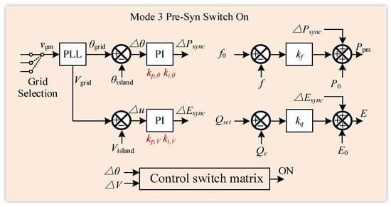
Before closing the mechanical switch to establish Path 1, the converter must bring its output voltage into synchronism with the target normally operating grid. This pre-synchronization mode is activated when the system decides to close the switch, as shown in Figure 6. The outer layer still uses the frequency droop and reactive droop of Mode 2 as the baseline but adds two PI regulators that adjust the mechanical power command and the voltage amplitude based on the measured phase and amplitude errors.

Figure 6. Block diagrams of Mode 3.

Let the phase error be defined as $\mathsf{\Delta }\theta ={\theta }_{\mathrm{g}\mathrm{r}\mathrm{i}\mathrm{d}}-{\theta }_{\mathrm{i}\mathrm{s}\mathrm{l}\mathrm{a}\mathrm{n}\mathrm{d}}$. The electromagnetic power of the VSG can be linearized around the equilibrium point. Considering the power–angle relationship $\delta ={\theta }_{\mathrm{i}\mathrm{s}\mathrm{l}\mathrm{a}\mathrm{n}\mathrm{d}}-{\theta }_{\mathrm{g}\mathrm{r}\mathrm{i}\mathrm{d}}=-\mathsf{\Delta }\theta$, we have $P_e\approx P_{\mathrm{l}\mathrm{o}\mathrm{a}\mathrm{d}}+K_s\delta =P_{\mathrm{l}\mathrm{o}\mathrm{a}\mathrm{d}}-K_s\mathsf{\Delta }\theta$, where $K_s=\left(V_{\mathrm{g}\mathrm{r}\mathrm{i}\mathrm{d}}{V}_{\mathrm{i}\mathrm{s}\mathrm{l}\mathrm{a}\mathrm{n}\mathrm{d}}\right)/X$ is the synchronizing power coefficient. This sign correction is essential to reflect that when $\mathsf{\Delta }\theta >0$ (grid phase leading), the VSG outputs less electromagnetic power.

The mechanical power command in pre-synchronization mode is given by (8), which can be rewritten as

$$P_{\mathrm{p}\mathrm{m}}=P_0+k_{\omega }({\omega }_{\mathrm{r}\mathrm{e}\mathrm{f}}-{\omega }_0)$$

(8)

with the frequency reference

$${\omega }_{\mathrm{r}\mathrm{e}\mathrm{f}}={\omega }_0+k_{p,\theta }\mathsf{\Delta }\theta +k_{i,\theta }\int \mathsf{\Delta }\theta dt.$$

(9)

Here, $k_{\omega }$ is the frequency–power droop coefficient (in W·s/rad). At steady state, $P_0=P_{\mathrm{l}\mathrm{o}\mathrm{a}\mathrm{d}}$. Hence, the small-signal variation of the mechanical power is

$$\mathsf{\Delta }{P}_{\mathrm{p}\mathrm{m}}=k_{\omega }\left(k_{p,\theta }\mathsf{\Delta }\theta +k_{i,\theta }\int \mathsf{\Delta }\theta dt\right).$$

(10)

The VSG swing equation, including the damping term $D$ explicitly, is

$$J{\displaystyle \frac{d\omega }{dt}}={\displaystyle \frac{P_{\mathrm{p}\mathrm{m}}-P_e}{\omega }}-D(\omega -{\omega }_0).$$

(11)

Linearizing around the rated angular frequency ${\omega }_0$ and substituting the power expressions yields

$$J{\displaystyle \frac{d\mathsf{\Delta }\omega }{dt}}={\displaystyle \frac{1}{{\omega }_0}}[\mathsf{\Delta }{P}_{\mathrm{p}\mathrm{m}}-\mathsf{\Delta }{P}_e]-D\mathsf{\Delta }\omega ,$$

(12)

with $\mathsf{\Delta }{P}_e=-K_s\mathsf{\Delta }\theta$ and $\mathsf{\Delta }\omega =\omega -{\omega }_0$.

Defining the state variables $x_1=\mathsf{\Delta }\theta$, $x_2=\mathsf{\Delta }\omega$, and $x_3=\int \mathsf{\Delta }\theta dt$, the linearized system becomes

$$\begin{array}{cc}{\dot{x}}_1& =x_2,\\ {\dot{x}}_2& =-{\displaystyle \frac{D}{J}}{x}_2+{\displaystyle \frac{k_{\omega }{k}_{p,\theta }+K_s}{J{\omega }_0}}{x}_1+{\displaystyle \frac{k_{\omega }{k}_{i,\theta }}{J{\omega }_0}}{x}_3,\\ {\dot{x}}_3& =x_1.\end{array}$$

(13)

The characteristic equation is obtained from $\mathrm{d}\mathrm{e}\mathrm{t}(sI-A)=0$:

$$s^3+{\displaystyle \frac{D}{J}}{s}^2-{\displaystyle \frac{k_{\omega }{k}_{p,\theta }+K_s}{J{\omega }_0}}s-{\displaystyle \frac{k_{\omega }{k}_{i,\theta }}{J{\omega }_0}}=0.$$

(14)

To ensure all coefficients are positive, the second-order term must carry a minus sign. We therefore rewrite the equation in standard form by factoring a negative sign in the linear-order coefficient, which leads to a stable system only when additional sign conventions are met. Actually, a clearer derivation shows that the correct sign for the $s$ term should be positive if we define the state variables consistently. Let us re-derive the A matrix with the corrected $P_e$ sign:

From $\mathsf{\Delta }{P}_e=-K_s\mathsf{\Delta }\theta$, the difference $\mathsf{\Delta }{P}_{\mathrm{p}\mathrm{m}}-\mathsf{\Delta }{P}_e=k_{\omega }{k}_{p,\theta }\mathsf{\Delta }\theta +k_{\omega }{k}_{i,\theta }{x}_3-(-K_s\mathsf{\Delta }\theta )=(k_{\omega }{k}_{p,\theta }+K_s)\mathsf{\Delta }\theta +k_{\omega }{k}_{i,\theta }{x}_3$.

Therefore,

$${\dot{x}}_2=-{\displaystyle \frac{D}{J}}{x}_2+{\displaystyle \frac{k_{\omega }{k}_{p,\theta }+K_s}{J{\omega }_0}}{x}_1+{\displaystyle \frac{k_{\omega }{k}_{i,\theta }}{J{\omega }_0}}{x}_3.$$

(15)

The state matrix is

$$A=\left[\begin{array}{ccc}0& 1& 0\\ {\displaystyle \frac{k_{\omega }{k}_{p,\theta }+K_s}{J{\omega }_0}}& -{\displaystyle \frac{D}{J}}& {\displaystyle \frac{k_{\omega }{k}_{i,\theta }}{J{\omega }_0}}\\ 1& 0& 0\end{array}\right].$$

(16)

The characteristic polynomial follows:

$$\mathrm{d}\mathrm{e}\mathrm{t}(sI-A)=s^3+{\displaystyle \frac{D}{J}}{s}^2-{\displaystyle \frac{k_{\omega }{k}_{p,\theta }+K_s}{J{\omega }_0}}s-{\displaystyle \frac{k_{\omega }{k}_{i,\theta }}{J{\omega }_0}}=0.$$

(17)

For stability, the coefficients of the polynomial $s^3+a_2{s}^2+a_{1}s+a_0=0$ must all be positive. Here, $a_2=D/J>0$, but $a_1=-(k_{\omega }{k}_{p,\theta }+K_s)/\left(J{\omega }_0\right)$ and $a_0=-k_{\omega }{k}_{i,\theta }/\left(J{\omega }_0\right)$. Since $k_{p,\theta },k_{i,\theta },K_s,k_{\omega }$ are all positive, both $a_1$ and $a_0$ are negative, indicating an unstable system. This reveals a sign mistake in the definition of the feedback loop: the phase PI should act to reduce the phase error, requiring negative feedback. Hence, the correct frequency reference should be

$${\omega }_{\mathrm{r}\mathrm{e}\mathrm{f}}={\omega }_0-k_{p,\theta }\mathsf{\Delta }\theta -k_{i,\theta }\int \mathsf{\Delta }\theta dt.$$

(18)

With this correction, $\mathsf{\Delta }{P}_{\mathrm{p}\mathrm{m}}=-k_{\omega }(k_{p,\theta }\mathsf{\Delta }\theta +k_{i,\theta }{x}_3)$. Then

$$\mathsf{\Delta }{P}_{\mathrm{p}\mathrm{m}}-\mathsf{\Delta }{P}_e=-k_{\omega }{k}_{p,\theta }\mathsf{\Delta }\theta -k_{\omega }{k}_{i,\theta }{x}_3-(-K_s\mathsf{\Delta }\theta )=(K_s-k_{\omega }{k}_{p,\theta })\mathsf{\Delta }\theta -k_{\omega }{k}_{i,\theta }{x}_3.$$

(19)

Now,

$${\dot{x}}_2=-{\displaystyle \frac{D}{J}}{x}_2+{\displaystyle \frac{K_s-k_{\omega }{k}_{p,\theta }}{J{\omega }_0}}{x}_1-{\displaystyle \frac{k_{\omega }{k}_{i,\theta }}{J{\omega }_0}}{x}_3.$$

(20)

The state matrix becomes

$$A=\left[\begin{array}{ccc}0& 1& 0\\ {\displaystyle \frac{K_s-k_{\omega }{k}_{p,\theta }}{J{\omega }_0}}& -{\displaystyle \frac{D}{J}}& -{\displaystyle \frac{k_{\omega }{k}_{i,\theta }}{J{\omega }_0}}\\ 1& 0& 0\end{array}\right].$$

(21)

The characteristic equation is

$$s^3+{\displaystyle \frac{D}{J}}{s}^2+{\displaystyle \frac{k_{\omega }{k}_{p,\theta }-K_s}{J{\omega }_0}}s+{\displaystyle \frac{k_{\omega }{k}_{i,\theta }}{J{\omega }_0}}=0.$$

(22)

Routh–Hurwitz stability conditions: All coefficients must be positive, and the inequality $a_2{a}_1>a_0$ must hold.

$$a_2={\displaystyle \frac{D}{J}}>0,a_1={\displaystyle \frac{k_{\omega }{k}_{p,\theta }-K_s}{J{\omega }_0}},a_0={\displaystyle \frac{k_{\omega }{k}_{i,\theta }}{J{\omega }_0}}.$$

(23)

Therefore, we require:

$$k_{\omega }{k}_{p,\theta }>K_s(\mathrm{to} \mathrm{make} a_1>0),$$

(24)

$$k_{i,\theta }>0,$$

$${\displaystyle \frac{D}{J}}\cdot {\displaystyle \frac{k_{\omega }{k}_{p,\theta }-K_s}{J{\omega }_0}}>{\displaystyle \frac{k_{\omega }{k}_{i,\theta }}{J{\omega }_0}}\Rightarrow k_{i,\theta }<{\displaystyle \frac{D(k_{\omega }{k}_{p,\theta }-K_s)}{J{k}_{\omega }}}.$$

Pole placement design: With the damping term included, the characteristic polynomial now possesses all three terms, allowing for arbitrary pole placement. Choosing a desired third-order polynomial

$$(s+\zeta {\omega }_n)(s^2+2\zeta {\omega }_{n}s+{\omega }_n^2)=s^3+3\zeta {\omega }_n{s}^2+(2{\zeta }^2{\omega }_n^2+{\omega }_n^2)s+\zeta {\omega }_n^3,$$

(25)

and equating coefficients, we obtain the design formulas:

$$\begin{array}{cc}{\displaystyle \frac{D}{J}}& =3\zeta {\omega }_n\Rightarrow {\omega }_n={\displaystyle \frac{D}{3\zeta J}},\\ {\displaystyle \frac{k_{\omega }{k}_{p,\theta }-K_s}{J{\omega }_0}}& =2{\zeta }^2{\omega }_n^2+{\omega }_n^2={\omega }_n^2(2{\zeta }^2+1),\\ {\displaystyle \frac{k_{\omega }{k}_{i,\theta }}{J{\omega }_0}}& =\zeta {\omega }_n^3.\end{array}$$

(26)

From these, the PI gains are explicitly given by

$$k_{p,\theta }={\displaystyle \frac{K_s+J{\omega }_0{\omega }_n^2(2{\zeta }^2+1)}{k_{\omega }}},k_{i,\theta }={\displaystyle \frac{J{\omega }_0\zeta {\omega }_n^3}{k_{\omega }}}$$

(27)

The damping ratio $\zeta$ can be selected between 0.7 and 1.0, and ${\omega }_n$ is determined by the physical damping $D$ and inertia $J$. These formulas guarantee both stability and specified dynamic performance.

3.4. Mode 4: Power Transfer Mode for Opening the Mechanical Switch (Power Transfer Mode)

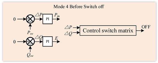
A mechanical switch must never be opened while carrying significant current, as this would cause arcing and severe transients. Therefore, before opening the mechanical switch, for example, when switching the source grid from a normally operating grid to a new one, the power flowing through Path 1 must be reduced to zero gradually. This is achieved by a closed-loop feedback control, as shown in Figure 7.

Figure 7. Block diagrams of Mode 4.

In this power transfer mode, the converter operates in grid-connected mode (Mode 1), but its power command is no longer given by the short-time-scale optimization. Instead, the outer layer continuously measures the active power $P_{\mathrm{sw}}$ and reactive power $Q_{\mathrm{sw}}$ flowing through the mechanical switch (i.e., through Path 1). The goal is to drive both $P_{\mathrm{sw}}$ and $Q_{\mathrm{sw}}$ to zero. A PI regulator is used to generate the mechanical power command $P_m$ and the internal voltage amplitude $E$:

$$\begin{array}{cccc}& P_{pm}=k_{p,P}\cdot (0-P_{\mathrm{sw}})+k_{i,P}\int (0-P_{\mathrm{sw}}) dt,& & \end{array}$$

(28)

$$\begin{array}{cccc}& E=E_0+k_{p,Q}\cdot (0-Q_{\mathrm{sw}})+k_{i,Q}\int (0-Q_{\mathrm{sw}}) dt.& & \end{array}$$

(29)

Here, $E_0$ is the nominal voltage amplitude, which is typically 1 p.u. The feedforward term in Mode 1 is replaced by these PI outputs. As the converter adjusts its output according to the PI commands, the power flowing through the mechanical switch gradually decreases. The DC bus voltage is automatically maintained by other converters, such as power-taking units or the energy storage converter, through their droop responses. Once the measured power falls below a small threshold,

$$\begin{array}{cccc}& \left|P_{\mathrm{sw}}\right|\le {\epsilon }_P\cdot P_{\mathrm{rated}},\left|Q_{\mathrm{sw}}\right|\le {\epsilon }_Q\cdot Q_{\mathrm{rated}},& & \end{array}$$

(30)

with ${\epsilon }_P$ and ${\epsilon }_Q$ typically set to 0.01, and the control system determines that the path is safe to open. It then sends an open command to the mechanical switch.

After the switch is opened, the converter transitions to Mode 2 (off-grid mode) if the off-grid side is isolated or remains in Mode 1 if another mechanical source is already connected.

3.5. Protection and Switching Coordination

Safe mechanical switching requires careful attention to several practical aspects. The mechanical switch is closed only when the voltage amplitude error and phase angle error both fall below preset thresholds, which are chosen to limit the worst-case inrush current within the making capacity of standard breakers. The inherent closing delay of mechanical switches (tens of milliseconds) is tolerated because the VSG inertia keeps the phase drift negligible during this short interval. For opening, a dead time is inserted after the current is driven to zero, ensuring the switch is fully open before a new path is established and preventing any momentary paralleling of asynchronous sources. Protection coordination is maintained by blocking mechanical switching when a fault is detected on the off-grid side, by relying on standard overcurrent relays during normal parallel operation, and by instantly isolating a faulted source grid to avoid back-feed. Finally, a state-machine-based interlocking logic prevents switch conflicts in the M × N matrix: at most one switch per row and per column can be closed, and every switching sequence follows a break-before-make rule. These measures together ensure that the proposed reconfiguration method operates reliably and remains fully compatible with existing distribution protection practices.

4. Two-Time-Scale Power Path Dynamic Allocation Strategy

Based on the seamless reconfiguration technology presented in Section 3, this section proposes a two-time-scale power path dynamic allocation strategy to coordinate long-term economy and short-term responsiveness. On the long time scale (T_Long), which is typically one hour, the source grid for the mechanical direct path called Path 1 is optimally selected, and the required mode transition sequences are executed using the four control modes defined in Section 3. On the short time scale (T_Short), ranging from seconds to minutes, after the mechanical path is fixed, the remaining power is automatically allocated between the third-party grid path called Path 2 and the energy storage path called Path 3 by tuning the DC voltage droop parameters of the AC-DC converters.

4.1. Long Time Scale: Grid Selection and Switching Execution for Path 1

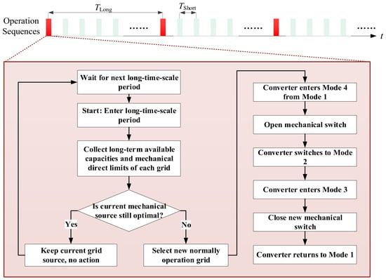
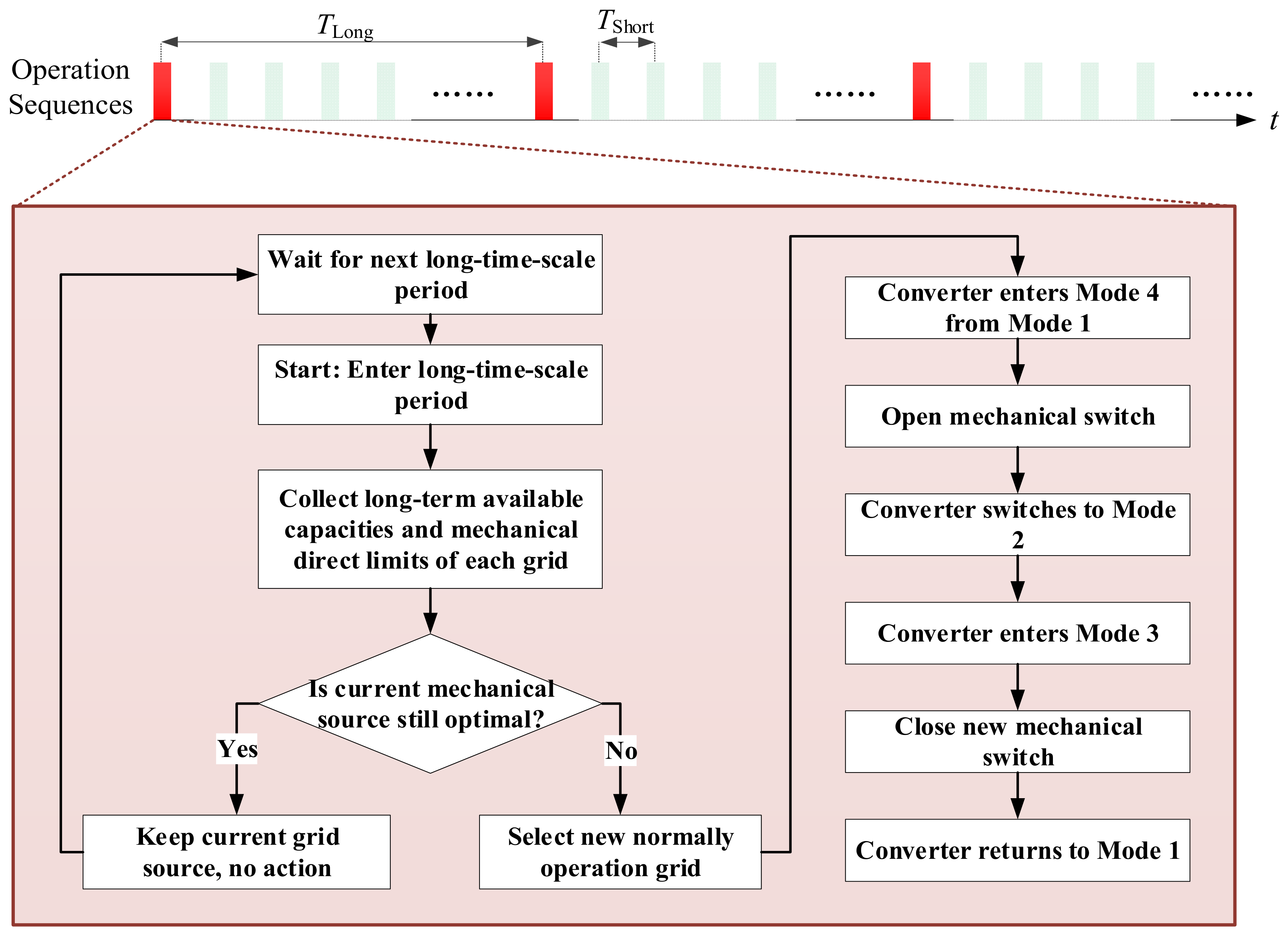
The long-time-scale optimization shown in Figure 8 decides which normally operating grid serves as the mechanical source for Path 1. This decision is made based on the long-term available capacities of each grid and is updated at a slow rate, for example, every hour, to avoid frequent mechanical switch operations.

Figure 8. The flow chart of the long-time-scale strategy.

4.1.1. Source Grid Selection

Let the off-grid grid be number 1 and the set of normally operating grids be $\mathcal{M}=\{2,3,\dots ,M\}$. Each grid $m$ has a long-term available power limit $P_{m,\mathrm{avail}}^{\mathrm{long}}$ considering predicted load and generation and a maximum mechanical direct power $P_{m,\mathrm{line},\max }$ limited by feeder capacity. Define a binary variable $z_m$ indicating whether grid $m$ is selected as the mechanical source, with ${\sum }_{m\in \mathcal{M}}{z}_m\le 1$.

The objective is to minimize the long-term operating cost, including losses and possible electricity price differences. For simplicity, a heuristic rule can be used: select the grid whose $P_{m,\mathrm{line},\max }$ is greater than the average load and which has the largest remaining capacity. When the current mechanical source becomes inadequate or another grid becomes significantly more advantageous, a switch is triggered.

4.1.2. Switching Execution Using Mode Transitions

The switching process involves two typical scenarios: initial establishment of Path 1 after a grid outage and switching from an old mechanical source to a new one. Both scenarios rely on the four control modes defined in Section 3.

Initial establishment of Path 1. Initially, the converter operates in Mode 2, forming a stable AC voltage to supply the isolated load. When the system decides to close the mechanical switch to a normally operating grid, the converter enters Mode 3. In this pre-synchronization mode, the phase and amplitude PI regulators drive the voltage errors to zero. Once the phase, voltage, and frequency differences fall within their thresholds, the mechanical switch closes with negligible inrush current. The converter then switches to Mode 1, where the mechanical power command is determined by DC voltage droop control with a feedforward term from the short-time-scale optimization. Path 1 now carries the base load, and the remaining power is handled by Path 2 and Path 3.

Switching from an old source to a new source. Suppose Path 1 is initially connected to grid 2. The converter, still in Mode 1, is commanded to enter Mode 4. In this power transfer mode, the outer layer uses closed-loop PI control based on the measured power through the mechanical switch, gradually reducing that power to zero. Once the power falls below a safe threshold, the old mechanical switch is opened without arcing. The converter then transitions to Mode 2, resuming off-grid operation to maintain uninterrupted supply to the load. Next, the system identifies the new target grid, and the converter enters Mode 3 to synchronize its voltage with the new grid. After synchronization, the new mechanical switch is closed, establishing the new Path 1. Finally, the converter returns to Mode 1, and the short-time-scale optimization re-allocates the remaining power among Path 2 and Path 3.

All mode transitions rely on the shared inner VSG, voltage, and current loops, which remain active throughout, ensuring seamless behavior.

4.2. Short Time Scale: Power Allocation Between Path 2 and Path 3 via Droop Parameter Optimization

After Path 1 is fixed and carries a mechanical power $P_{\mathrm{m}\mathrm{e}\mathrm{c}\mathrm{h}}$, the remaining load $P_{\mathrm{i}\mathrm{n}\mathrm{v}}=P_{\mathrm{l}\mathrm{o}\mathrm{a}\mathrm{d}}-P_{\mathrm{m}\mathrm{e}\mathrm{c}\mathrm{h}}$ must be supplied by Path 2 (third-party grid path) and Path 3 (energy storage path). The power flows of both paths converge to the common DC bus. The DC bus power balance is

$$\begin{array}{cccc}& {\displaystyle \sum _{m\in \mathcal{M}}}{P}_{\mathrm{s}\mathrm{r}\mathrm{c},m}+P_{\mathrm{e}\mathrm{s}\mathrm{s}}=P_{\mathrm{i}\mathrm{n}\mathrm{v}},& & \end{array}$$

(31)

where $P_{\mathrm{s}\mathrm{r}\mathrm{c},m}\ge 0$ is the DC power injected from grid $m$ via an AC-DC converter, and $P_{\mathrm{e}\mathrm{s}\mathrm{s}}$ is the energy storage power (positive for discharging and negative for charging).

The short-time-scale optimization determines the power set points that minimize the instantaneous total cost, subject to all relevant physical and operational constraints. The complete formulation is as follows:

Objective function:

The total cost includes conversion losses, electricity purchase cost, and battery degradation:

$$\begin{array}{cccc}& \mathrm{m}\mathrm{i}\mathrm{n} {\displaystyle \sum _{m\in \mathcal{M}}}({\beta }_{\mathrm{a}\mathrm{c}\mathrm{d}\mathrm{c}}+{\rho }_m)P_{\mathrm{s}\mathrm{r}\mathrm{c},m}+c_{\mathrm{e}\mathrm{s}\mathrm{s},\mathrm{d}\mathrm{i}\mathrm{s}}\cdot P_{\mathrm{e}\mathrm{s}\mathrm{s}}^{+}+c_{\mathrm{e}\mathrm{s}\mathrm{s},\mathrm{c}\mathrm{h}}\cdot P_{\mathrm{e}\mathrm{s}\mathrm{s}}^{-}& & \end{array}$$

(32)

where ${\beta }_{\mathrm{a}\mathrm{c}\mathrm{d}\mathrm{c}}=1/{\eta }_{\mathrm{a}\mathrm{c}\mathrm{d}\mathrm{c}}-1\approx 0.05$ is the loss coefficient for the AC-DC-AC path. ${\rho }_m$ is the electricity price or carbon emission cost of grid $m$ (can be zero if unavailable). $P_{\mathrm{e}\mathrm{s}\mathrm{s}}^{+}=\mathrm{m}\mathrm{a}\mathrm{x}(P_{\mathrm{e}\mathrm{s}\mathrm{s}},0)$ and $P_{\mathrm{e}\mathrm{s}\mathrm{s}}^{-}=\mathrm{m}\mathrm{a}\mathrm{x}(-P_{\mathrm{e}\mathrm{s}\mathrm{s}},0)$ separate discharging and charging power. $c_{\mathrm{e}\mathrm{s}\mathrm{s},\mathrm{d}\mathrm{i}\mathrm{s}}={\beta }_{\mathrm{e}\mathrm{s}\mathrm{s},\mathrm{d}\mathrm{i}\mathrm{s}}+c_{\mathrm{d}\mathrm{e}\mathrm{g}}$ and $c_{\mathrm{e}\mathrm{s}\mathrm{s},\mathrm{c}\mathrm{h}}={\beta }_{\mathrm{e}\mathrm{s}\mathrm{s},\mathrm{c}\mathrm{h}}-c_{\mathrm{d}\mathrm{e}\mathrm{g}}$. Here, ${\beta }_{\mathrm{e}\mathrm{s}\mathrm{s},\mathrm{d}\mathrm{i}\mathrm{s}}\approx 0.06$ and ${\beta }_{\mathrm{e}\mathrm{s}\mathrm{s},\mathrm{c}\mathrm{h}}\approx 0.03$ are the loss coefficients for the storage path, and $c_{\mathrm{d}\mathrm{e}\mathrm{g}}$ is the linearized battery degradation cost per kWh of throughput. This formulation correctly captures that degradation cost reduces the effective cost of charging (since charging adds energy that can be used later) and increases the cost of discharging.

Converter capacity limits:

$$0\le P_{\mathrm{s}\mathrm{r}\mathrm{c},m}\le P_{m,\mathrm{s}\mathrm{r}\mathrm{c},\mathrm{m}\mathrm{a}\mathrm{x}},\forall m\in \mathcal{M}.$$

Energy storage power limits with SOC dynamics: The storage power must respect both the converter rating and the state-of-charge limits:

$$P_{\mathrm{e}\mathrm{s}\mathrm{s},\mathrm{c}\mathrm{h},\mathrm{m}\mathrm{a}\mathrm{x}}\left(SOC\right)\le P_{\mathrm{e}\mathrm{s}\mathrm{s}}\le P_{\mathrm{e}\mathrm{s}\mathrm{s},\mathrm{d}\mathrm{i}\mathrm{s},\mathrm{m}\mathrm{a}\mathrm{x}}\left(SOC\right),$$

where:

$$\begin{array}{cc}{P}_{\mathrm{e}\mathrm{s}\mathrm{s},\mathrm{d}\mathrm{i}\mathrm{s},\mathrm{m}\mathrm{a}\mathrm{x}}\left(SOC\right)& =\mathrm{m}\mathrm{i}\mathrm{n}\left(P_{\mathrm{r}\mathrm{a}\mathrm{t}\mathrm{e}\mathrm{d}}, {\displaystyle \frac{SOC-SO{C}_{\mathrm{m}\mathrm{i}\mathrm{n}}}{\mathsf{\Delta }t}} E_{\mathrm{c}\mathrm{a}\mathrm{p}}\right),\\ P_{\mathrm{e}\mathrm{s}\mathrm{s},\mathrm{c}\mathrm{h},\mathrm{m}\mathrm{a}\mathrm{x}}\left(SOC\right)& =-\mathrm{m}\mathrm{i}\mathrm{n}\left(P_{\mathrm{r}\mathrm{a}\mathrm{t}\mathrm{e}\mathrm{d}}, {\displaystyle \frac{SO{C}_{\mathrm{m}\mathrm{a}\mathrm{x}}-SOC}{\mathsf{\Delta }t}} E_{\mathrm{c}\mathrm{a}\mathrm{p}}\right),\end{array}$$

with $E_{\mathrm{c}\mathrm{a}\mathrm{p}}$ the rated energy capacity and $\mathsf{\Delta }t$ the optimization interval.

To ensure that the storage can instantly take over the full load if Path 1 fails, an upward reserve margin is maintained:

$$P_{\mathrm{e}\mathrm{s}\mathrm{s}}+R_{\mathrm{u}\mathrm{p}}\le P_{\mathrm{e}\mathrm{s}\mathrm{s},\mathrm{d}\mathrm{i}\mathrm{s},\mathrm{m}\mathrm{a}\mathrm{x}}\left(SOC\right),R_{\mathrm{u}\mathrm{p}}=\alpha \cdot P_{\mathrm{i}\mathrm{n}\mathrm{v}},$$

where $\alpha \in [0,1]$ is the reserve coefficient (e.g., 0.2). A downward reserve may be added analogously if needed.

Feeder thermal limits: For each source grid, the line flow must not exceed its emergency rating:

$$P_{\mathrm{s}\mathrm{r}\mathrm{c},m}\le P_{m,\mathrm{l}\mathrm{i}\mathrm{n}\mathrm{e},\mathrm{m}\mathrm{a}\mathrm{x}}-P_{m,\mathrm{o}\mathrm{t}\mathrm{h}\mathrm{e}\mathrm{r}},$$

where $P_{m,\mathrm{o}\mathrm{t}\mathrm{h}\mathrm{e}\mathrm{r}}$ is the non-controllable load on that feeder. This constraint is usually ensured by the long-time-scale selection and may be omitted in the short-time-scale LP.

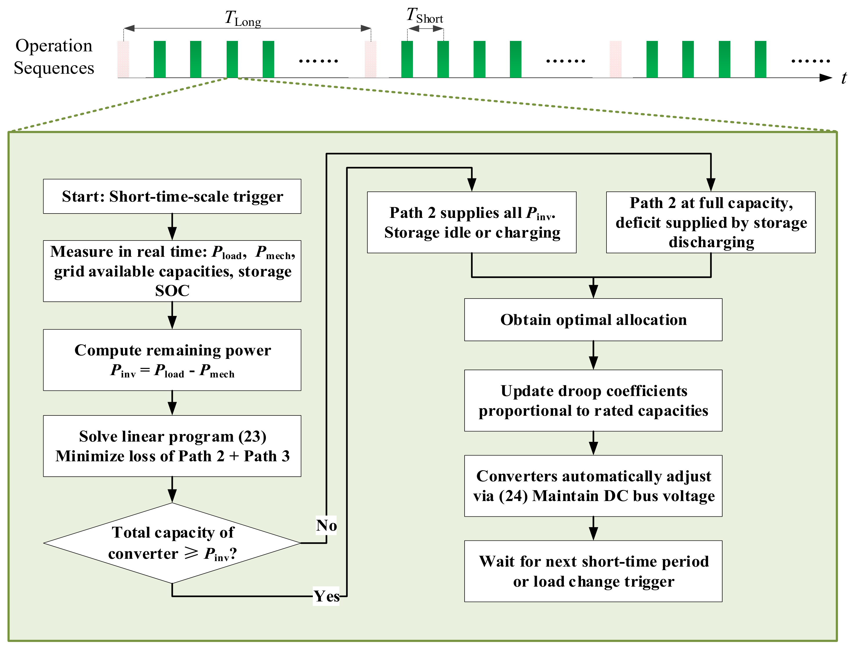
The above problem is a small-scale linear program. It can be solved analytically in most practical cases because the loss coefficients and prices satisfy ${\beta }_{\mathrm{a}\mathrm{c}\mathrm{d}\mathrm{c}}+{\rho }_m<c_{\mathrm{e}\mathrm{s}\mathrm{s},\mathrm{d}\mathrm{i}\mathrm{s}}$ under normal conditions. The optimal strategy is as follows:

(1)

Use Path 2 as much as possible up to the total converter capacity ${\sum }_m{P}_{m,\mathrm{s}\mathrm{r}\mathrm{c},\mathrm{m}\mathrm{a}\mathrm{x}}$ or the feeder limits, as it has the lowest marginal cost.

(2)

If Path 2 capacity is insufficient, discharge the energy storage ($P_{\mathrm{e}\mathrm{s}\mathrm{s}}>0$) subject to its discharge limit and reserve constraint.

(3)

If surplus Path 2 capacity exists and the storage is not fully charged, charge the storage ($P_{\mathrm{e}\mathrm{s}\mathrm{s}}<0$) at the optimal rate, respecting the charge limit.

The resulting optimal power set points $P_{\mathrm{s}\mathrm{r}\mathrm{c},m}^{*}$ and $P_{\mathrm{e}\mathrm{s}\mathrm{s}}^{*}$ are then used as the feedforward commands $P_{\mathrm{d}\mathrm{c}}^{\mathrm{f}\mathrm{f}}$ in the droop control law of each Mode 1 converter. The droop coefficients $k_{\mathrm{d}\mathrm{c}}$ are chosen proportional to the rated capacities, ensuring that any real-time mismatch is shared autonomously without communication.

The optimization is triggered periodically (e.g., every minute) or when the load changes beyond a threshold. The corresponding flow chart is shown in Figure 9.

Figure 9. The flow chart of the short-time-scale strategy.

5. Experimental Verification

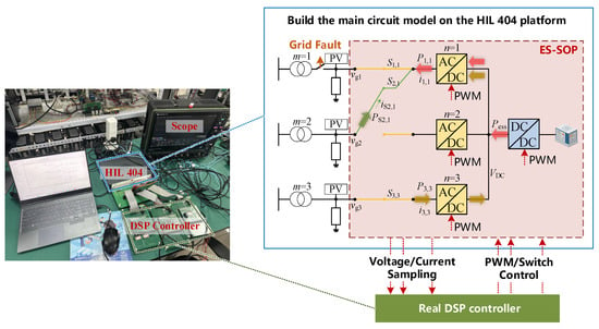
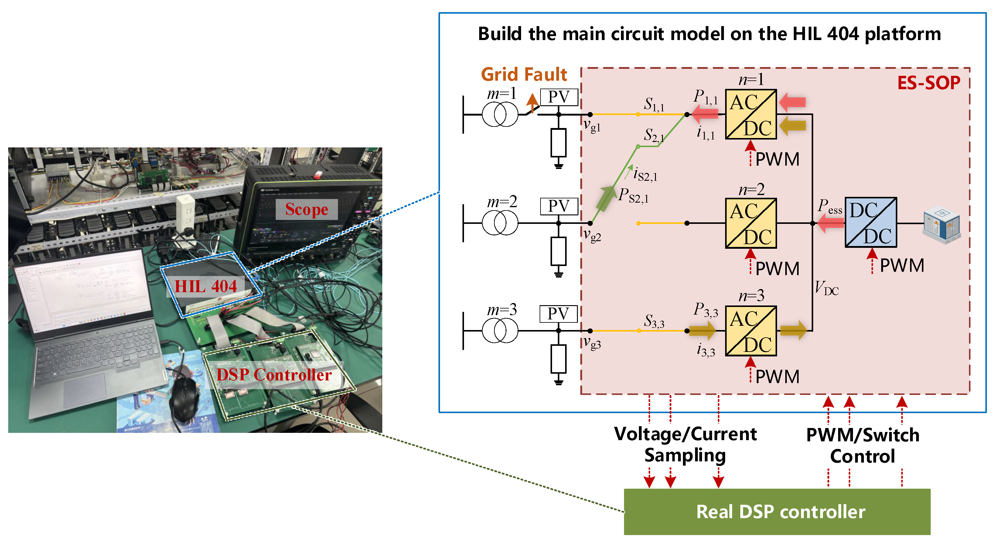
The proposed methods are validated through hardware-iItn-the-loop (HIL) experiments conducted on the Typhoon HIL 404 platform. The application scenario and the experimental setup are illustrated in Figure 10. HIL simulation is a well-established technique capable of accurately replicating practical operating conditions, and it supports signal interaction with DSP devices via AO and DI interfaces, which has gained widespread recognition in the field of power electronics. Since this research focuses on control strategy design, the combined DSP and HIL architecture is sufficient to verify the effectiveness of the proposed algorithm. The power circuit model is constructed inside the Typhoon HIL 404, while the control algorithm is programmed on a physical DSP chip. The platform transmits sampled voltage and current signals to the DSP via its built-in analog output (AO) ports. After algorithm calculation inside the DSP, PWM signals and switching commands for the switch matrix are generated. These signals are then sent back to the circuit model in Typhoon HIL 404 through the digital input (DI) ports, forming a complete hardware-in-the-loop simulation system. The experimental parameters are given in Table 3.

Figure 10. Typhoon HIL 404 experimental platform and system topology.

Table 3. The experimental parameters.

Parameters	Values
Converter ratings	30 kW
DC bus voltage	800 V
Grid voltage	220 V
Load levels	0–30 kW
Line impedances	10 μH
Storage capacity/SOC limits	200 Ah, max = 95%, min = 10%
Switching thresholds	$\mathsf{\Delta }\theta <3^{\circ }\mathsf{\Delta }V<5\mathrm{V}$
PI gains (voltage control loop)	KP = 3, KI = 10
PI gains (current control loop)	KP = 50, KI = 100
VSG parameters	J = 1/0.057 kg × m2 D = 15 N × ms/rad
Droop coefficients	500
Sampling time	10−4 s
Mechanical switch delay	20–100 ms

Three experiments are performed. Experiment 1 focuses on validating the effectiveness of the pre-synchronization mode within the seamless reconfiguration technology. Experiment 2 verifies the stability of the entire system during mode transitions, especially the DC voltage stability. Experiment 3 demonstrates the flexible power allocation among the three paths using the two-time-scale power path dynamic allocation strategy.

5.1. Experiment 1: Validation of the Pre-Synchronization Mode

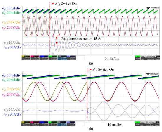
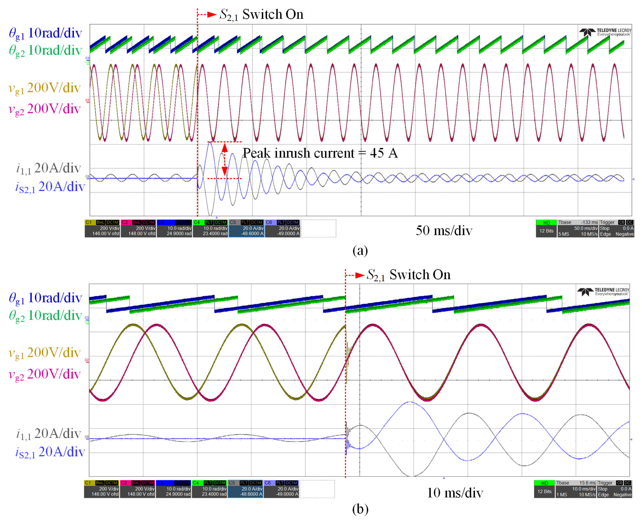
First, the scenario without the proposed method is examined. When grid 1 goes off-grid due to a fault, its connected converter must urgently switch to off-grid support mode. A few seconds later, mechanical switch $S_{2,1}$ is closed. Without pre-synchronization, an inevitable phase and voltage difference exists between the off-grid grid 1 and the normally operating grid 2. Closing the switch causes a large current inrush, which may trip the switch and impose severe power shocks on both the tie-line and the converters, potentially damaging the converters. The corresponding waveforms are shown in Figure 11, where ${\theta }_{g1}$ and ${\theta }_{g2}$ are the phases of grid 1 and grid 2, $v_{g1}$ and $v_{g2}$ are the phase-a voltages of the two grids, $P_{1,1}$ is the active power injected by converter 1 into grid 1 (i.e., Path 2 power), and $P_{S2,1}$ is the active power injected from grid 2 into grid 1 through the mechanical switch (i.e., Path 1 power). As shown in the figure, the peak inrush current reaches as high as 45 A before pre-synchronization is applied, and the settling time for the system to return to steady state is 100 ms.

Figure 11. (a) Experimental waveforms of θ_g1, θ_g2, v_g1, v_g2, i_1,1, and i_S2,1 without pre-synchronization method. (b) Zoomed view of (a).

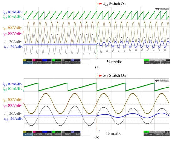
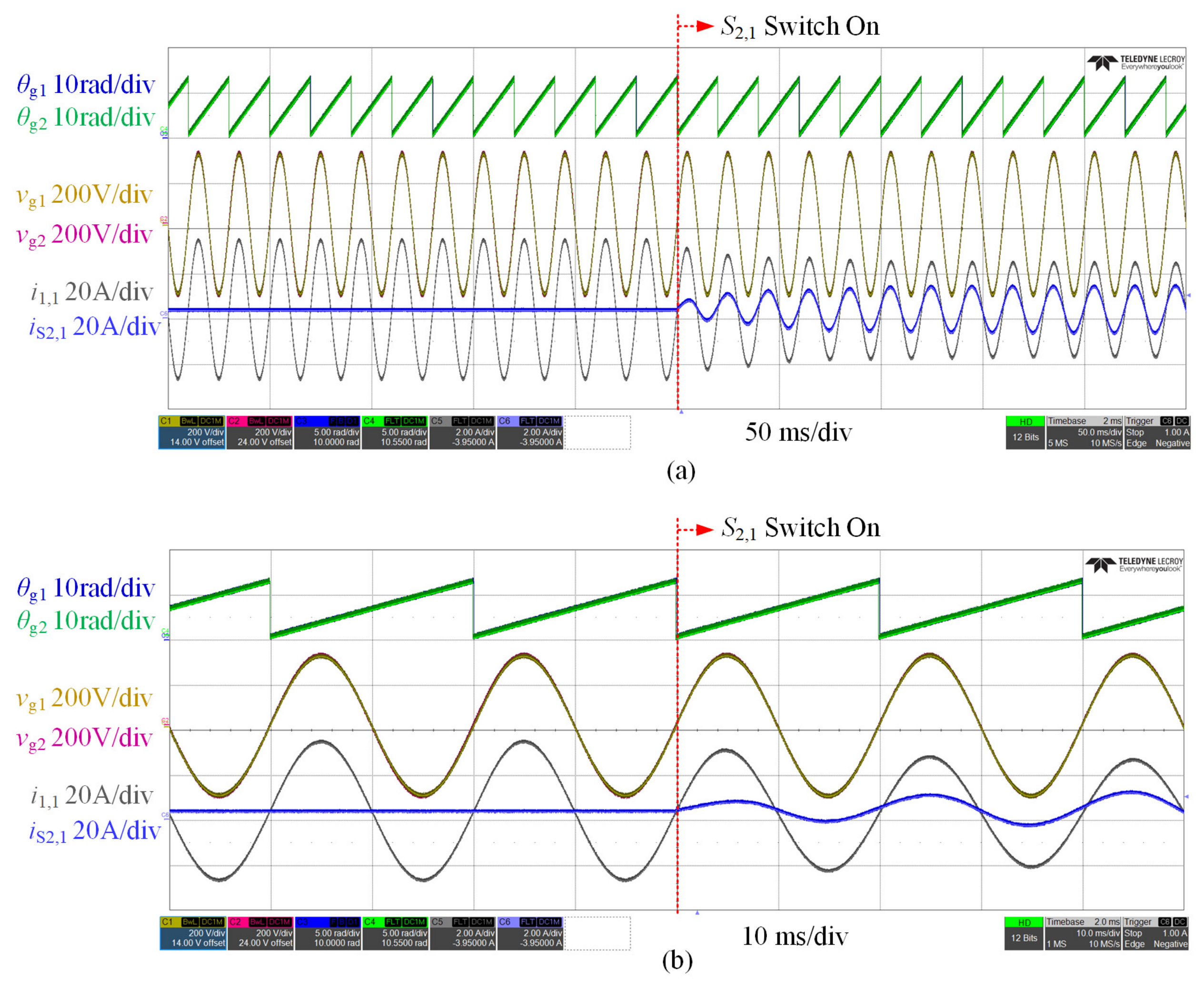
Next, the proposed method is applied. Under the same fault condition, AC/DC converter 1 not only supports the off-grid side but also achieves phase and voltage synchronization between grid 1 and grid 2 within one second. When mechanical switch $S_{2,1}$ is closed, no power surge occurs; part of the power is smoothly transferred to $S_{2,1}$. Thus, seamless reconfiguration among multiple paths is realized. The corresponding waveforms are shown in Figure 12. As shown in the figure, the peak inrush current is nearly eliminated after pre-synchronization is applied. The settling time to return to the steady state is less than 20 ms.

Figure 12. (a) Experimental waveforms of θ_g1, θ_g2, v_g1, v_g2, i_1,1, and i_S2,1 with pre-synchronization method. (b) Zoomed view of (a).

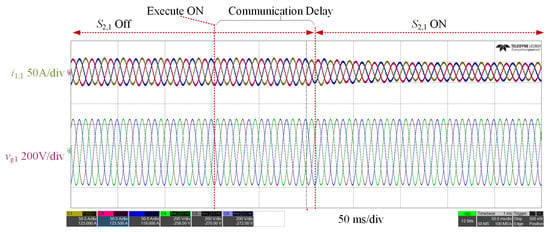
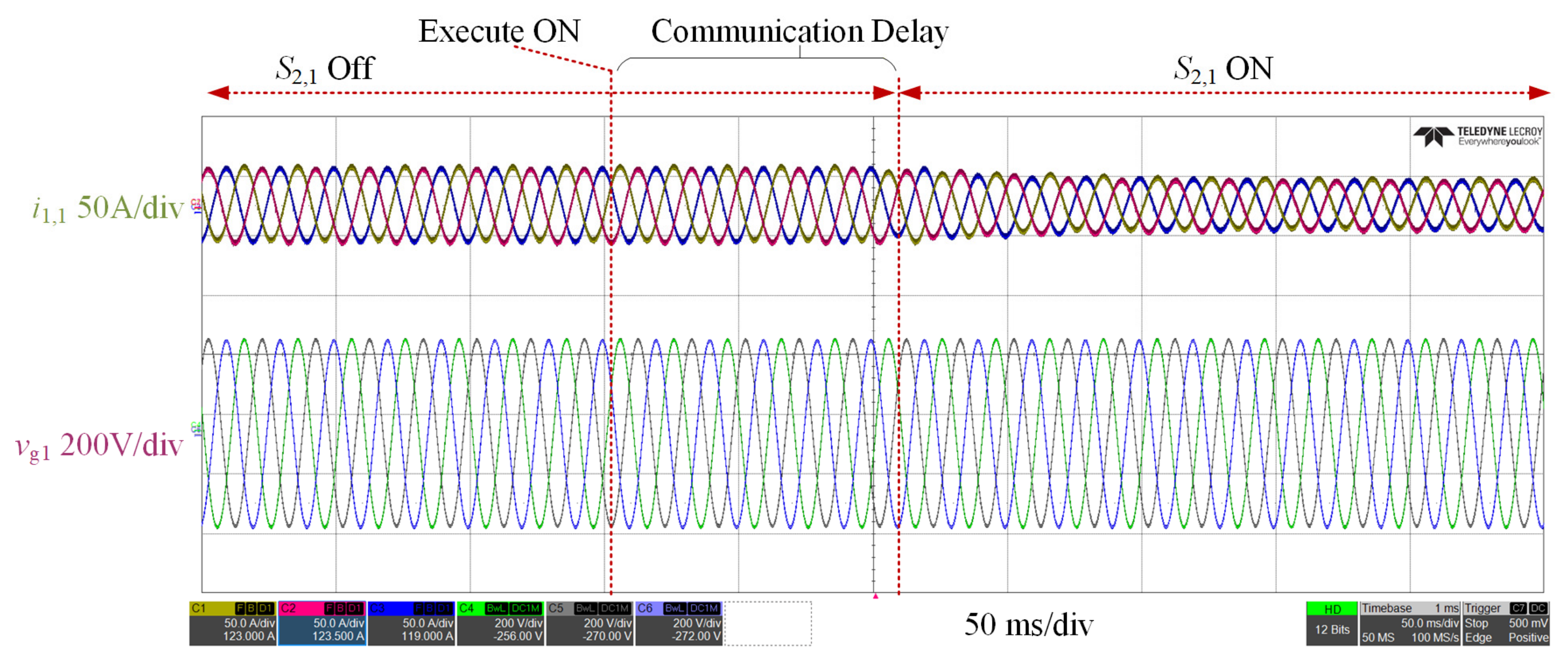
As shown in Figure 13, switch S_2,1 is initially open. All power of grid 1 is carried by converter 1. After the completion of pre-synchronization, an ON command is sent to S_2,1. Following a communication delay of 100–150 ms, S_2,1 is closed. Part of the power is then undertaken by S_2,1, resulting in a decrease in i_1,1. Therefore, the communication delay only affects the switching instant and exerts no substantial impact on the normal operation of the system.

Figure 13. Experimental waveforms of i_1,1 and v_g,1 with considering communication delay.

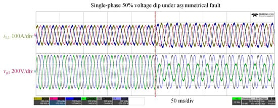
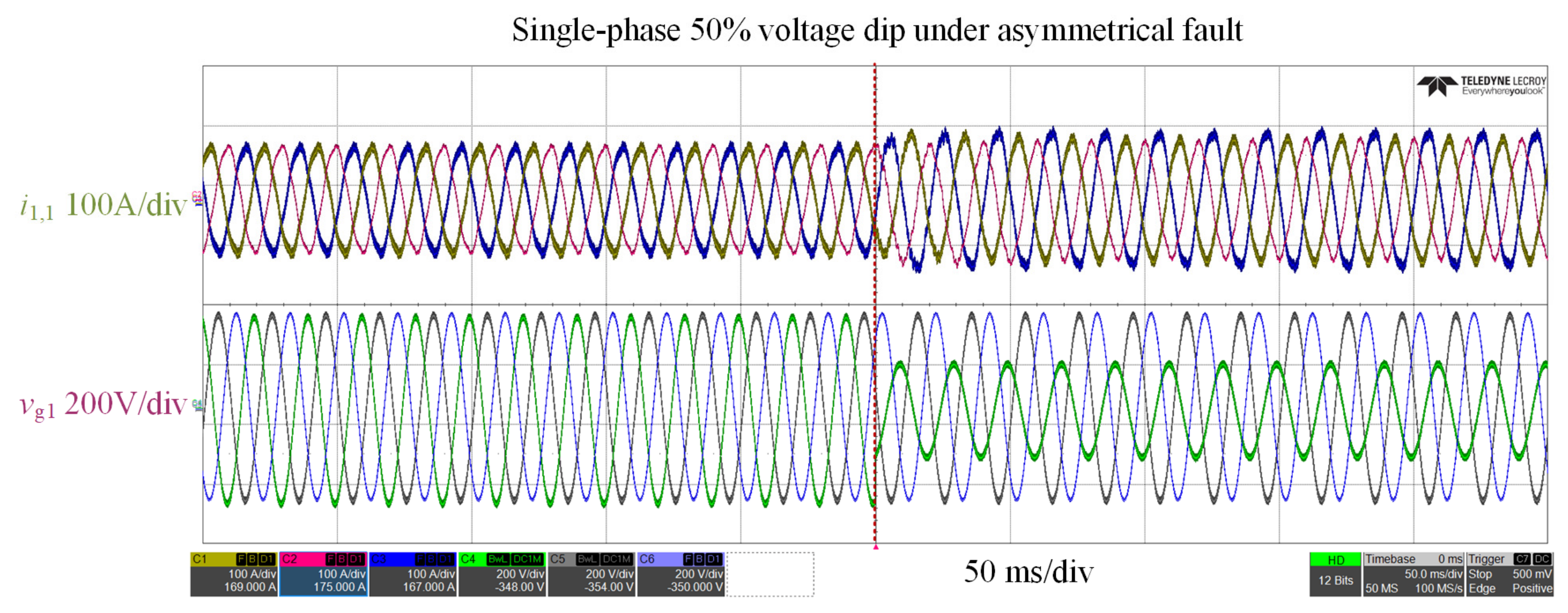
Figure 14 shows the response under asymmetrical fault with single-phase 50% voltage dip. The converter output restores to normal after a short transient process.

Figure 14. Experimental waveforms of i_1,1 and v_g1 under unbalanced faults.

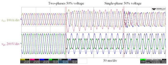
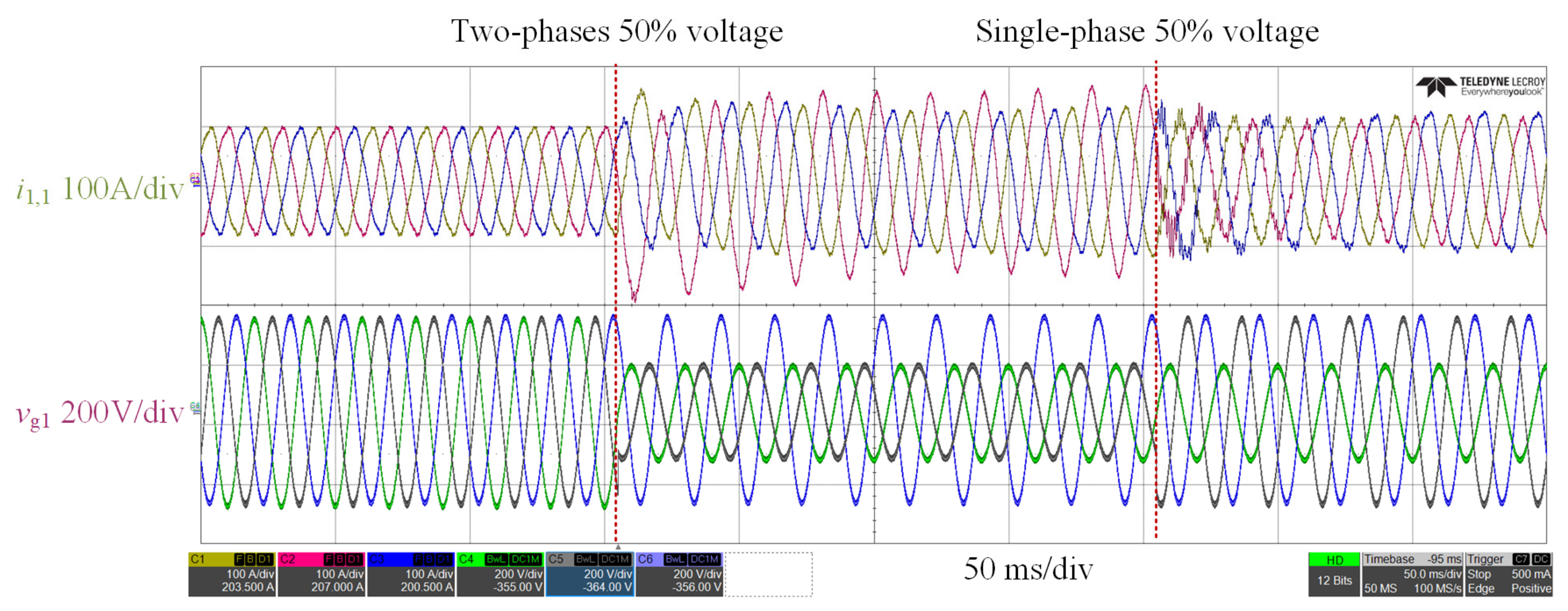
Assume that a two-phase voltage dip occurs initially, followed by a single-phase voltage dip. After a brief transient process, the converter output can return to normal in both cases, as shown in Figure 15.

Figure 15. Experimental waveforms of i_1,1 and v_g1 under multiple simultaneous grid faults.

5.2. Experiment 2: DC Bus Stability Verification

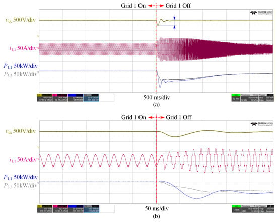
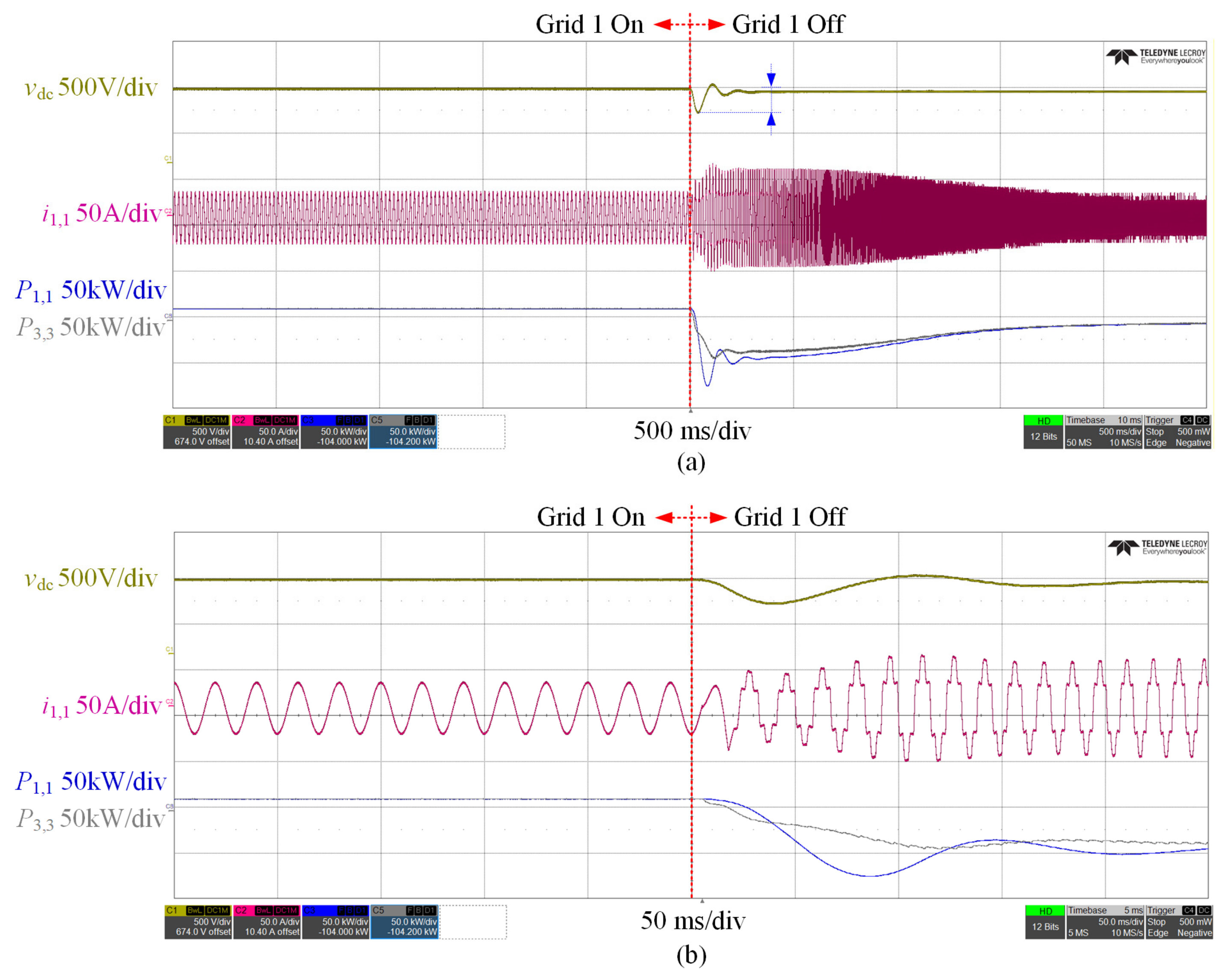
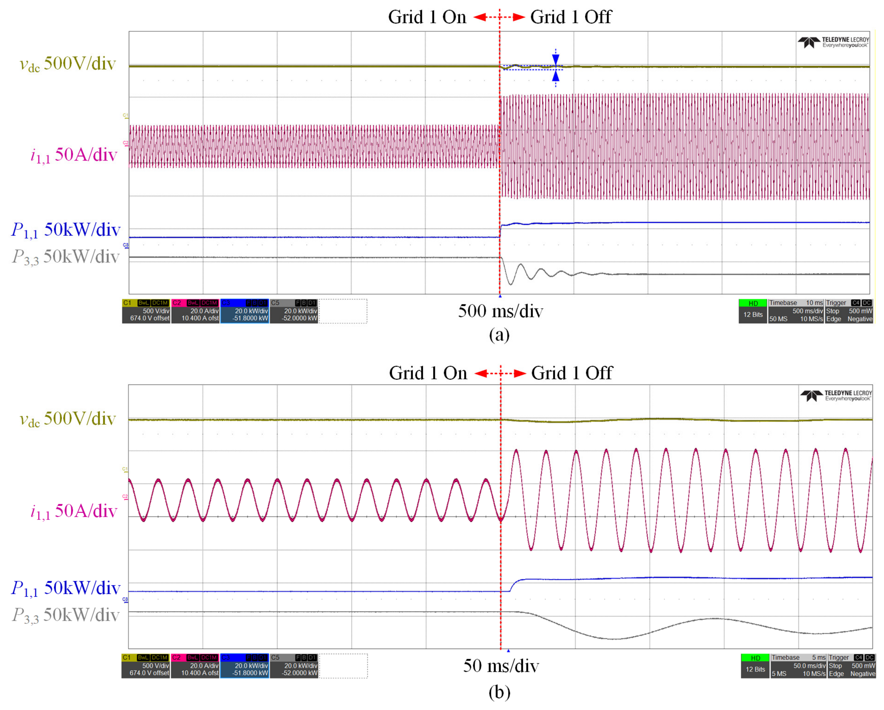
In practice, flexible interconnection devices often assign one AC/DC converter to regulate the DC voltage, ensuring system stability. However, when the grid connected to that converter suddenly goes off-grid, the converter must switch to grid-support mode, and the DC voltage control must be taken over by other converters. In real engineering, there is a delay, which may cause large DC voltage fluctuations or even collapse. In Figure 16, v_dc is the DC voltage, $i_{1,1}$ is the current injected by converter 1 into grid 1, $P_{1,1}$ is the active power of converter 1, and $P_{3,3}$ is the active power of converter 3. As shown in the figure, the DC voltage fluctuation exceeds 200 V. Low DC voltage makes the AC/DC converter unstable. This will eventually cause the whole system to collapse. The converter also generates power oscillation. At the same time, current harmonics increase.

Figure 16. (a) Experimental waveforms of v_dc, i_1,1, P_1,1, and P_3,3 with traditional DC voltage control method. (b) The zoomed view of (a).

With the proposed control scheme, multiple AC/DC converters and the DC/DC converter of the energy storage all participate in DC bus regulation. Therefore, when any grid connected to an AC/DC converter experiences an outage, the DC bus voltage remains stable with a fluctuation below 20 V. Meanwhile, the AC/DC converter still maintains high output power quality and shows no signs of instability, and the whole system can quickly enter a new steady state. The corresponding waveforms are shown in Figure 17.

Figure 17. (a) Experimental waveforms of v_dc, i_1,1, P_1,1, and P_3,3 with the proposed method. (b) The zoomed view of (a).

5.3. Experiment 3: Power Allocation Among Different Paths

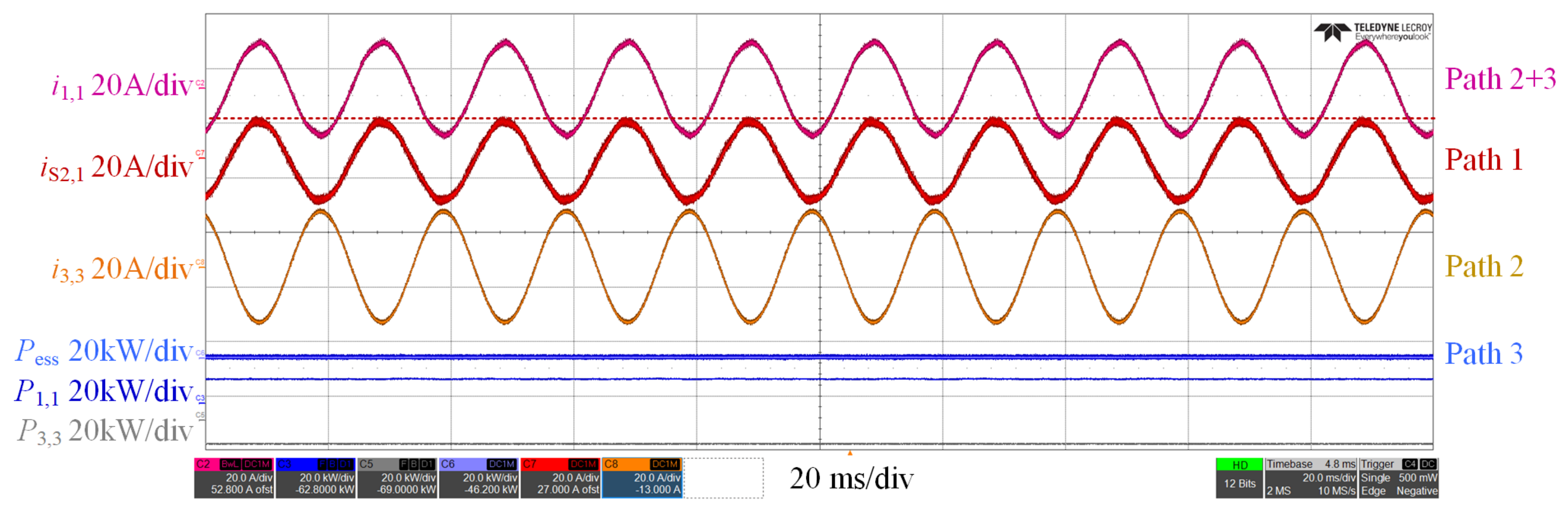
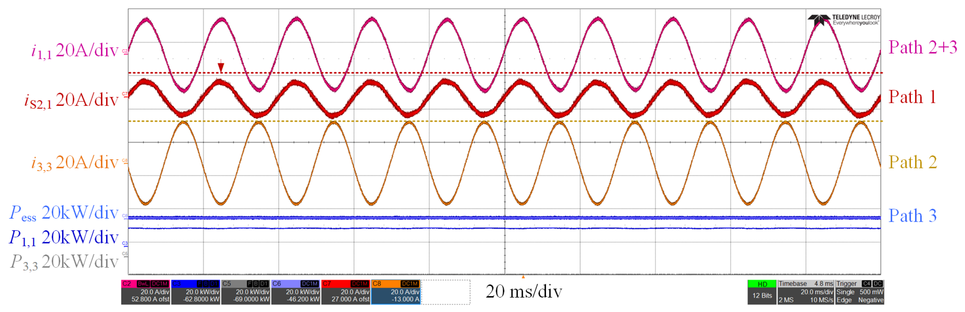
This experiment verifies the flexible allocation capability between Path 1 and Path 2. To fully exploit the low-loss advantage of Path 1, as much power as possible should be carried by Path 1, denoted by $i_{S2,1}$ in Figure 18. At this stage, Path 2 and Path 3 serve as the sources of supplementary power. If the power output of Path 2 is sufficient to meet the compensation demand, the battery power will be set to zero to minimize battery utilization P_ess. Since most of the power flows through Path 1, the corresponding power losses are negligible. Thus, the overall efficiency can exceed 98.5%. Meanwhile, the exact value is determined by the power ratio between Path 1 and Path 2.

Figure 18. Experimental waveforms of i_1,1, i_S2,3, i_3,3, and P_ess.

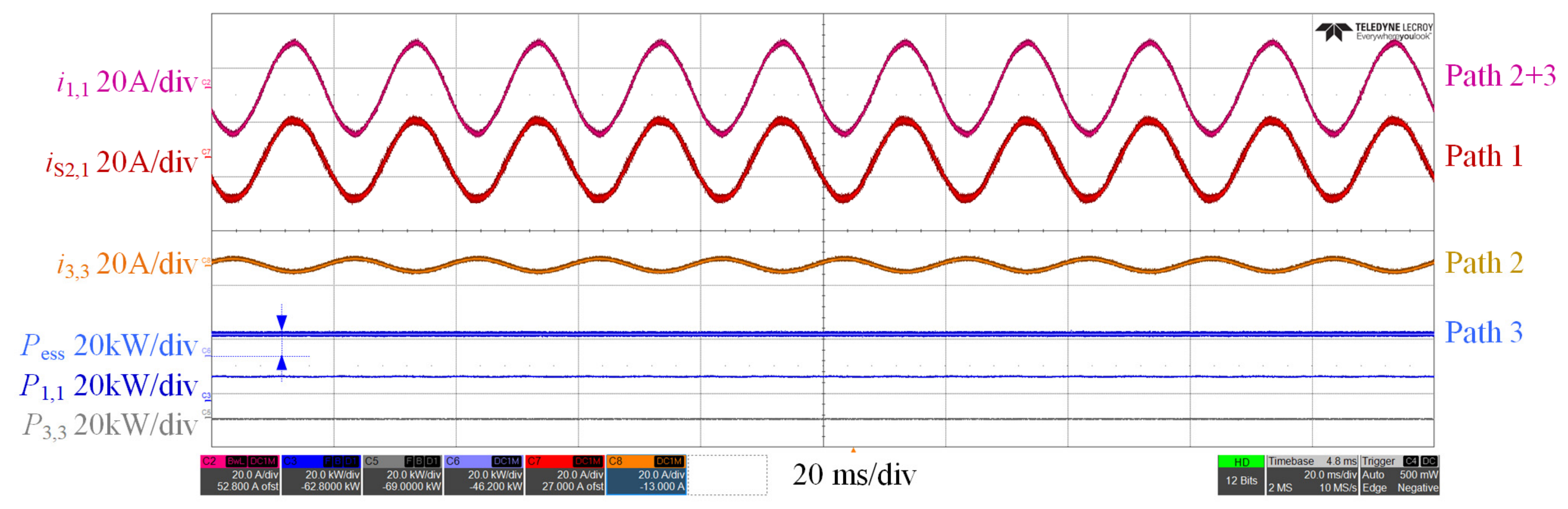
When the power available through Path 1 decreases, the power of Path 2, denoted by $i_{3,3}$, is increased to maintain support for the off-grid side, as shown in Figure 19. Furthermore, the flexible allocation capability of Path 3 is verified. When Path 1 and Path 2 are insufficient, the power of Path 3, represented by $P_{ess}$, is increased, as shown in Figure 20.

Figure 19. Experimental waveforms of i_1,1, i_S2,3, i_3,3, P_ess, P_1,1, and P_1,3 when reducing the power of Path 1.

Figure 20. Experimental waveforms of i_1,1, i_S2,3, i_3,3, P_ess, P_1,1, and P_1,3 when increasing the power of Path 3.

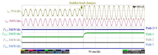
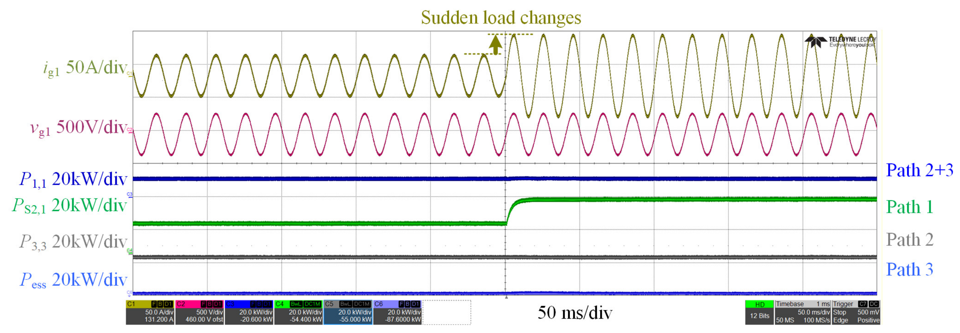
The waveforms under sudden load changes are presented in Figure 21. In this experiment, the load of distribution grid 1 was suddenly doubled, which caused an abrupt increase in i_g,1. The incremental power was undertaken by Path 1. As can be seen from the figure, P_S2,1 rises sharply to meet the demand brought by the sudden load increase of grid 1.

Figure 21. Experimental waveforms of i_g1, v_g1, P_1,1, P_S2,1, P_3,3, and P_ess under sudden load changes.

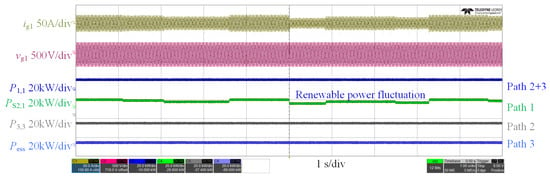
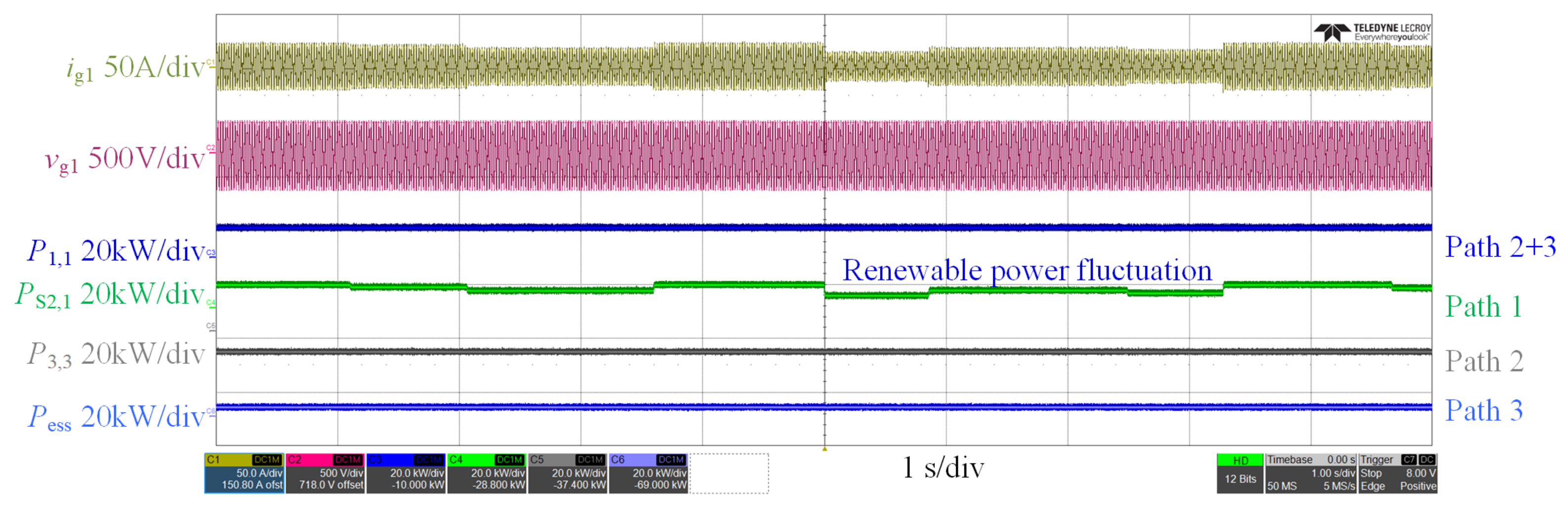
The waveforms under renewable power fluctuation are shown in Figure 22. The output of renewable energy in grid 1 fluctuates, which leads to the variation in i_g1. Such power fluctuations are mainly accommodated by Path 1. It can be observed that the power of P_S2,1 changes synchronously with the renewable energy output.

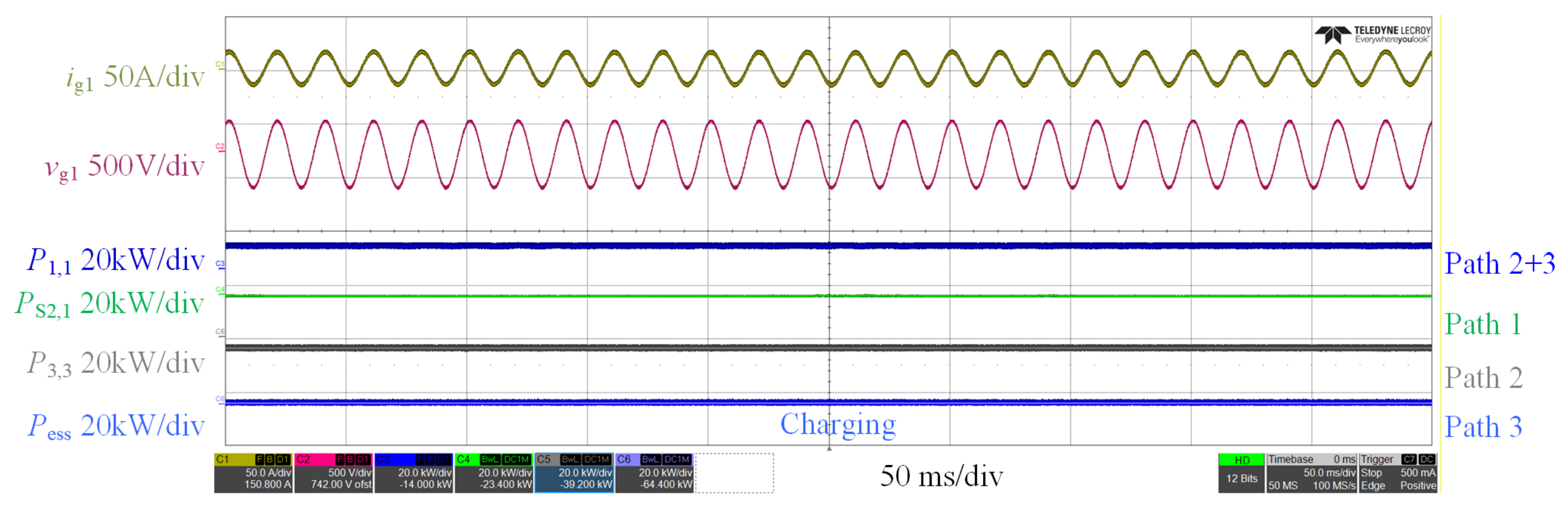
Figure 22. (a) Experimental waveforms of i_g1, v_g1, P_1,1, P_S2,1, P_3,3, and P_ess under renewable power fluctuation.

When the battery SOC is low, the battery can either cease operation or operate in charging mode. As shown in Figure 23, the primary task of ES-SOP under this condition is to provide emergency support for grid 1, so the energy storage system stops operating. When there is excess grid power, the battery can be charged to increase its SOC.

Figure 23. Experimental waveforms of i_g1, v_g1, P_1,1, P_S2,1, P_3,3, and P_ess under the condition of low battery SOC.

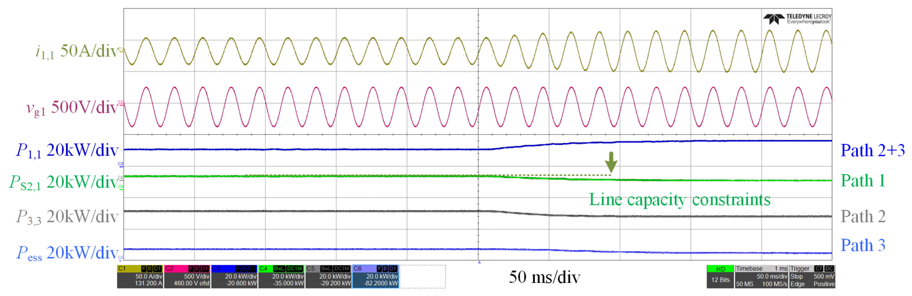
If Path 1 is subject to line capacity constraints, the power of Path 1 is curtailed, and the power of Path 3 is increased. As shown in Figure 24, i_1,1, P_1,1, and P_3,3 rise, while P_S2,1 decreases.

Figure 24. Experimental waveforms of i_1,1, v_g1, P_1,1, P_S2,1, P_3,3, and P_ess under line capacity constraints.

6. Conclusions

This paper presents a power path dynamic reconfiguration method for an energy storage-integrated soft open point (ES-SOP). The work makes three main contributions. First, a hybrid topology combines a mechanical direct path, a converter-based path, and an energy storage path through an M×N switch matrix. This structure largely avoids conversion losses by letting the base load flow through the mechanical path. Second, a seamless reconfiguration method is proposed. It uses four control modes to synchronize the off-grid side with the target grid before closing the mechanical switch, which completely removes inrush currents. Meanwhile, a DC bus droop coordination keeps the voltage fluctuation below 20 V during mode transitions. Third, a two-time-scale allocation strategy is developed. The long time scale selects the most suitable healthy grid for the mechanical path. The short time scale then shares the remaining power between the converter and storage paths by simply tuning the droop parameters, using only local measurements. Hardware-in-the-loop tests confirm that the method achieves approximately 98.5% transfer efficiency and ensures smooth, uninterrupted load transfer. Overall, the proposed ES-SOP provides a practical and robust solution for resilient distribution networks.

References

- Fuad, K.S.; Hafezi, H.; Kauhaniemi, K.; Laaksonen, H. Soft Open Point in Distribution Networks. IEEE Access 2020, 8, 210550–210565. [Google Scholar] [CrossRef] [Scilit]
- Li, P.; Ji, H.; Wang, C.; Zhao, J.; Song, G.; Ding, F.; Wu, J. Coordinated Control Method of Voltage and Reactive Power for Active Distribution Networks Based on Soft Open Point. IEEE Trans. Sustain. Energy 2017, 8, 1430–1442. [Google Scholar] [CrossRef] [Scilit]
- Ji, H.; Wang, C.; Li, P.; Ding, F.; Wu, J. Robust Operation of Soft Open Points in Active Distribution Networks with High Penetration of Photovoltaic Integration. IEEE Trans. Sustain. Energy 2019, 10, 280–289. [Google Scholar]
- Sun, F.; Ma, J.; Yu, M.; Wei, W. Optimized Two-Time Scale Robust Dispatching Method for the Multi-Terminal Soft Open Point in Unbalanced Active Distribution Networks. IEEE Trans. Sustain. Energy 2021, 12, 587–598. [Google Scholar]
- Sarantakos, I.; Peker, M.; Zografou-Barredo, N.-M.; Deakin, M.; Patsios, C.; Sayfutdinov, T.; Taylor, P.C.; Greenwood, D. A Robust Mixed-Integer Convex Model for Optimal Scheduling of Integrated Energy Storage–Soft Open Point Devices. IEEE Trans. Smart Grid 2022, 13, 4072–4087. [Google Scholar] [CrossRef] [Scilit]
- Wang, J.; Zhou, N.; Chung, C.Y.; Wang, Q. Coordinated Planning of Converter-Based DG Units and Soft Open Points Incorporating Active Management in Unbalanced Distribution Networks. IEEE Trans. Sustain. Energy 2020, 11, 2015–2027. [Google Scholar]
- Citroni, R.; Mangini, F.; Frezza, F. Efficient Integration of Ultra-low Power Techniques and Energy Harvesting in Self-Sufficient Devices: A Comprehensive Overview of Current Progress and Future Directions. Sensors 2024, 24, 4471. [Google Scholar] [CrossRef] [Scilit] [PubMed]
- Zhao, H.; Chen, W.; He, G.; Wang, J. A New Shared Module Soft Open Point for Power Distribution Network. IEEE Trans. Power Electron. 2023, 38, 3363–3374. [Google Scholar]
- Zhao, H.; Chen, W.; Lan, J.; Yuan, Y.; Xie, Y. A New Compact Soft Open Point Based on Cascaded H-Bridge and Mixed-Frequency Modulation. IEEE Trans. Power Electron. 2024, 39, 3363–3375. [Google Scholar]
- Jiang, X.; Zhou, Y.; Ming, W.; Yang, P.; Wu, J. An Overview of Soft Open Points in Electricity Distribution Networks. IEEE Trans. Smart Grid 2022, 13, 1899–1910. [Google Scholar] [CrossRef] [Scilit]
- Ivic, D.R.; Stefanov, P.C. An Extended Control Strategy for Weakly Meshed Distribution Networks with Soft Open Points and Distributed Generation. IEEE Access 2021, 9, 138220–138235. [Google Scholar] [CrossRef] [Scilit]
- Hafezi, H.; Laaksonen, H. Autonomous Soft Open Point Control for Active Distribution Network Voltage Level Management. In Proceedings of the 2019 IEEE Milan PowerTech, Milan, Italy, 23–27 June 2019; pp. 1–6. [Google Scholar]
- Olea-Oregi, E.; Eguía-López, P.; Sanchez-Ruiz, A.; Canas-Acena, J. Autonomous Active Power Dispatching Control of Soft Open Points in Distribution Networks. IEEE Trans. Smart Grid 2025, 16, 2081–2094. [Google Scholar] [CrossRef] [Scilit]
- Yang, X.; Xu, C.; Zhang, Y.; Yao, W.; Wen, J.; Cheng, S. Real-Time Coordinated Scheduling for ADNs with Soft Open Points and Charging Stations. IEEE Trans. Power Syst. 2021, 36, 5486–5499. [Google Scholar] [CrossRef] [Scilit]
- Sarantakos, I.; Zografou-Barredo, N.-M.; Huo, D.; Greenwood, D. A Reliability-Based Method to Quantify the Capacity Value of Soft Open Points in Distribution Networks. IEEE Trans. Power Syst. 2021, 36, 5032–5043. [Google Scholar] [CrossRef] [Scilit]
- Farzamnia, A.; Marjani, S.; Galvani, S.; Kin, K.T.T. Optimal Allocation of Soft Open Point Devices in Renewable Energy Integrated Distribution Systems. IEEE Access 2022, 10, 9309–9321. [Google Scholar] [CrossRef] [Scilit]
- You, R.; Lu, X. Voltage Unbalance Compensation in Distribution Feeders Using Soft Open Points. J. Mod. Power Syst. Clean Energy 2022, 10, 1000–1008. [Google Scholar] [CrossRef] [Scilit]
- Wang, Y.; Su, X.; Song, M.; Jiang, W.; Shahidehpour, M.; Xu, Q. Sequential Load Restoration With Soft Open Points and Time-Dependent Cold Load Pickup for Resilient Distribution Systems. IEEE Trans. Smart Grid 2023, 14, 3427–3438. [Google Scholar] [CrossRef] [Scilit]
- Yu, Y.; Shang, L.; Dong, X. A Control Strategy of Multi-Terminal Grid-Forming Soft Open Point for Uninterrupted Power Supply Under Feeder Power Outages. IEEE Trans. Power Electron. 2025, 40, 2642–2654. [Google Scholar]
- Lai, Z.; Yi, H.; Wang, Z.; Zhuo, F.; Zhuang, H. Transient Analysis and Overcurrent Limited Strategy for Supply Restoration-Oriented Hybrid Soft Open Point. IEEE Trans. Power Electron. 2024, 39, 2660–2676. [Google Scholar]
- Qian, T.; Ming, W.; Shao, C.; Hu, Q.; Wang, X.; Wu, J.; Wu, Z. An Edge Intelligence-Based Framework for Online Scheduling of Soft Open Points with Energy Storage. IEEE Trans. Smart Grid 2024, 15, 2934–2946. [Google Scholar]
- Wu, H.; Xu, Z.; Wang, M.; Jia, Y. Full-Model-Free Adaptive Graph Deep Deterministic Policy Gradient Model for Multi-Terminal Soft Open Point Voltage Control in Distribution Systems. J. Mod. Power Syst. Clean Energy 2024, 12, 1895–1907. [Google Scholar]
- Lu, M.; Mu, W.; Qin, M.; Koehler, A.; Fang, J.; Goetz, S.M. Differential Detection of Feeder and Mesh Impedances Through a Series-Parallel Direct-Injection Soft Open Point. IEEE Trans. Power Electron. 2025, 40, 1964–1973. [Google Scholar]
Disclaimer/Publisher’s Note: The statements, opinions and data contained in all publications are solely those of the individual author(s) and contributor(s) and not of MDPI and/or the editor(s). MDPI and/or the editor(s) disclaim responsibility for any injury to people or property resulting from any ideas, methods, instructions or products referred to in the content. |
© 2026 by the authors. Licensee MDPI, Basel, Switzerland. This article is an open access article distributed under the terms and conditions of the Creative Commons Attribution (CC BY) license.