A Physics-Informed Neural Network for the Design of Supersonic Turbine Stator Blades

Abstract

The recovery of low- and medium-temperature waste heat using Organic Rankine Cycles (ORCs) is increasingly important for improving the efficiency and sustainability of industrial and energy systems. In compact ORC turboexpanders, high specific power output and large pressure ratios often require single- or two-stage turbines operating in transonic or supersonic regimes. Under these conditions, stator blade design is complicated by strong compressible-flow effects and, for organic working fluids, by real-gas thermodynamic behavior. Conventional supersonic stator design methods, such as the method of characteristics, are mainly applicable to the diverging supersonic portion of the blade passage, while the converging region is typically defined using empirical or heuristic prescriptions. This paper presents a physics-informed neural-network-based design method for supersonic turbine stator blades. The proposed framework generates the complete inter-blade passage, including both the converging and diverging regions, starting from a prescribed mean-line geometry and Mach number distribution. The velocity field is obtained by solving the governing equations of steady, inviscid, adiabatic, irrotational compressible flow within a PINN formulation. A hard boundary-condition strategy is used to impose the specified mean-line velocity distribution exactly, while real-fluid thermodynamic effects are incorporated through lookup tables for the speed of sound and density. The blade contours are then reconstructed from stream-function isolines predicted from the computed velocity field. The method is demonstrated for two working fluids: air, treated as a perfect gas, and toluene undergoing transcritical expansion. The resulting blade passages are first validated using inviscid CFD simulations, which show close agreement between the prescribed and computed mean-line Mach number distributions. Turbulent CFD simulations of the final blade cascades confirm smooth acceleration through the inter-blade passage, with no strong internal shocks and only weak fishtail shocks downstream of the trailing edge. For both fluids, the post-expansion ratio is approximately unity and the exit flow angle remains close to the prescribed blade metal angle, indicating well-matched supersonic stator designs. The results demonstrate that the proposed PINN-based design method provides a physically consistent approach for generating supersonic stator blade profiles for both ideal-gas and real-gas turbine applications.

1. Introduction

The recovery of low- and medium-temperature waste heat has become an important route for improving the overall efficiency and sustainability of industrial and energy systems. Among the technologies available for this purpose, Organic Rankine Cycles (ORCs) are particularly attractive because they can convert heat from relatively low-temperature sources into mechanical or electrical power by using organic working fluids with suitable thermodynamic properties [1,2,3]. In compact ORC power systems, the turbine is often required to operate with high pressure ratios and large specific enthalpy drops [4,5]. As a result, efficient energy conversion may require single-stage or two-stage expanders in which the flow inside the stator and rotor blade passages becomes transonic or supersonic [6,7,8].

The aerodynamic design of ORC turbines is more challenging than that of conventional air or steam turbines because the expansion process may occur in thermodynamic regions where ideal-gas assumptions are no longer valid [9,10]. Organic fluids can exhibit strong real-gas and dense-gas effects, especially near the saturation line or in transcritical operating conditions [11,12]. These effects influence the speed of sound, Mach number distribution, pressure field, and shock structure, and therefore must be accounted for during blade design [9,11]. Previous studies on supersonic ORC turbines have emphasized that the design process requires accurate thermodynamic-property models and aerodynamic methods capable of treating non-ideal compressible-flow behavior [7,13]. Fast preliminary design procedures have therefore extended classical gas-dynamic tools, such as the method of characteristics, to fluids governed by general equations of state and to turbine passages affected by strong real-gas effects [13,14,15].

Supersonic turbine stator blades are commonly designed by prescribing the desired expansion and flow turning within the inter-blade passage. In traditional approaches, the method of characteristics is frequently used to construct the supersonic part of a nozzle or blade passage so that the desired outlet Mach number and flow direction are obtained while avoiding strong internal shocks [16,17,18]. However, this method is naturally suited to hyperbolic supersonic-flow regions and is not directly applicable to the subsonic or converging portion of the passage [15,18]. Consequently, the complete blade geometry is often obtained by combining characteristic-based design in the diverging region with empirical or heuristic prescriptions in the converging region [13,14,15]. This separation can limit design flexibility and may produce geometries that require further correction by computational fluid dynamics (CFD) simulations or shape optimization [7,14,15].

High-fidelity CFD has become an essential tool for evaluating and refining ORC turbine blade designs. It can capture complex compressible-flow phenomena, including expansion waves, shocks, viscous losses, and boundary-layer development [4,11,19]. Nevertheless, CFD-based optimization is computationally expensive because each candidate geometry requires mesh generation, numerical solution of the governing equations, and post-processing of the resulting flow field [19,20]. This cost becomes particularly significant when real-fluid thermodynamic models are included or when large design spaces must be explored [19,21]. Experimental validation is also limited because measurements in supersonic ORC cascades are difficult and require specialized facilities [22,23]. Recent experimental campaigns on linear cascades representative of ORC turbine stator nozzles have been developed to address this gap, but the available experimental database remains much smaller than that for conventional turbomachinery flows [22,23].

In parallel with developments in CFD and experimental methods, machine learning techniques have attracted increasing interest as surrogate models and design tools for fluid-dynamic applications [24,25,26]. Neural networks are capable of approximating nonlinear mappings between geometry, operating conditions, and flow quantities, and can therefore reduce the cost of repeated aerodynamic evaluations [27,28,29]. However, purely data-driven models generally require large training datasets and may produce predictions that violate physical constraints when extrapolated beyond the training domain [30,31,32]. This is a serious limitation in turbomachinery design, where the available high-fidelity data may be limited and where conservation laws, thermodynamic consistency, and boundary conditions must be satisfied [29,33].

Physics-informed neural networks (PINNs) offer a promising alternative by embedding the governing equations directly into the training process. In the PINN framework, the neural network is trained not only to match available data or boundary conditions, but also to minimize the residuals of the governing partial differential equations at collocation points distributed throughout the computational domain [30,31]. This approach was introduced as a general framework for solving forward and inverse problems involving nonlinear partial differential equations and has since been extended to many scientific and engineering applications [31,34]. For inverse aerodynamic design, a PINN is attractive because it can incorporate partial boundary information while using the governing equations to constrain the unknown flow field in regions where no direct data are available [35,36,37].

A further important issue in PINN-based flow modeling is the treatment of boundary conditions. In the original or “vanilla” PINN formulation, boundary conditions are usually enforced in a soft manner by adding boundary-error terms to the loss function [30,31]. Although this approach is simple and flexible, the resulting solution may not satisfy prescribed boundary conditions exactly, especially when the relative weights of the loss terms are difficult to tune [38,39]. Earlier neural-network approaches for solving differential equations introduced trial solutions that satisfy boundary conditions analytically [40,41], while more recent PINN formulations have used distance functions to impose boundary conditions exactly [38]. Such hard-enforcement strategies are particularly useful in inverse-design problems, where a specified mean-line velocity distribution or geometric constraint must be satisfied while the surrounding flow field and blade surfaces are reconstructed from the solution.

The present work develops a PINN-based method for supersonic turbine stator blades design. The proposed approach is motivated by the limitations of conventional method-of-characteristics-based design [14,15] and by the need for a systematic framework capable of treating both the converging and diverging regions of the blade passage. Instead of prescribing only the supersonic part of the passage, the method starts from a prescribed inter-blade mean line and a desired Mach number distribution along that line. The corresponding velocity distribution is obtained from isentropic-flow relations and real-fluid thermodynamic properties. A PINN is then trained to solve the governing equations of steady, inviscid, adiabatic, irrotational compressible flow in the regions above and below the mean line. The speed of sound and density are evaluated from thermodynamic-property lookup tables generated using a real-gas equation-of-state framework, enabling the method to be applied not only to air but also to organic working fluids such as toluene. CoolProp is used as the thermophysical-property library because it provides accurate property evaluations for pure and pseudo-pure fluids and has been widely used in ORC and refrigeration simulations [42].

The principal novelty of the proposed method is the use of a PINN to reconstruct a two-dimensional compressible velocity field in the vicinity of a prescribed passage mean line. A key feature of the formulation is its unified treatment of both the converging and diverging regions of the passage. The prescribed velocity distribution along the mean line is enforced exactly through a hard boundary condition, while the governing equations constrain the solution throughout the surrounding flow domain. The reconstructed velocity field is subsequently used to determine the stream-function field, whose selected isolines define the pressure and suction sides of the blade passage. In this way, the blade geometry is derived directly from a physics-constrained flow solution rather than from a purely empirical geometric construction.

The contributions of this work can be summarized as follows. First, a PINN-based design framework is formulated for supersonic turbine stator blades operating with either ideal-gas or real-gas working fluids. Second, the governing equations of steady, irrotational compressible flow are coupled with thermodynamic-property lookup tables, allowing real-fluid effects to be incorporated through the speed of sound and density. Third, a hard boundary-condition strategy is introduced to enforce the prescribed mean-line velocity distribution exactly. Finally, the blade profile is reconstructed from stream-function isolines and evaluated using CFD simulations, demonstrating the ability of the proposed method to generate smooth supersonic stator passages consistent with the imposed design specifications.

In addition to the steady aerodynamic design, unsteady wakes and their interaction with shocks and downstream blade rows play an important role in the performance of the turbomachinery. Wake evolution is associated with mixing losses, turbulence generation, periodic flow distortion, and complex wake–shock interactions, particularly in transonic and supersonic blade passages. A recent review [43] provides a comprehensive discussion of unsteady wake characteristics, evolution mechanisms, aerodynamic losses, and modern experimental and numerical analysis techniques in turbomachinery. Data-driven and reduced-order methods are also increasingly used to identify coherent structures and dominant temporal scales in complex turbomachinery flows. For example, reduced-order variational mode decomposition has been applied to transient flow fields in a mixed-flow pump, demonstrating the potential of modal methods for extracting physically relevant flow structures from high-dimensional data [44]. Although the present study is restricted to the reconstruction of a steady, inviscid compressible flow field for stator-blade design, such unsteady and data-driven analysis methods provide promising directions for extending the proposed framework to wake evolution, shock–wake interactions, and transient blade-row flows.

The remainder of this paper is organized as follows. Section 2 presents the mathematical model for steady, compressible, irrotational flow and the treatment of thermodynamic properties. Section 3 describes the proposed PINN-based design procedure, including the definition of the mean line, the prescribed Mach number distribution, the PINN formulation, stream-function reconstruction, and blade-profile generation. Section 4 presents the resulting blade designs and their CFD-based validation for air and toluene. Finally, Section 5 summarizes the main conclusions and outlines possible directions for future work.

2. Mathematical Model

In this study, a planar nozzle is considered under choked-flow conditions, undergoing steady isentropic expansion from the reservoir thermodynamic state to supersonic conditions. The flow is further assumed to be inviscid and adiabatic, with no shocks present in the flow field. Under these assumptions, the specific total enthalpy per unit mass, $h_0$, and the specific entropy per unit mass, s, are uniform throughout the entire flow field. Accordingly, the governing equations for steady, compressible, irrotational flow can be applied:

$$(v_x^2-c^2){\displaystyle \frac{\partial v_x}{\partial x}}+(v_y^2-c^2){\displaystyle \frac{\partial v_y}{\partial y}}+2v_x{v}_y{\displaystyle \frac{\partial v_x}{\partial y}}=0,$$

(1)

$${\displaystyle \frac{\partial v_x}{\partial y}}-{\displaystyle \frac{\partial v_y}{\partial x}}=0,$$

(2)

where $(x,y)$ are the Cartesian spatial coordinates, $v_x$ and $v_y$ are the corresponding Cartesian components of the velocity vector, and c is the local speed of sound.

The thermodynamic properties of the fluid enter the governing equations solely through the speed of sound c, as defined by the selected equation of state (EoS). For flows with uniform total enthalpy $h_0$ and entropy s, the speed of sound may be written as

$$c=c(s,h)=c\left(h\right),$$

(3)

since the entropy is constant. Moreover, the static enthalpy is related to the velocity magnitude by

$$h=h_0-{\displaystyle \frac{{\left|\mathbf{v}\right|}^2}{2}},$$

(4)

so h, and therefore c, depend only on $\left|\mathbf{v}\right|$.

Once the velocity field has been determined, the stream-function field can be reconstructed. The stream-function iso-lines then represent the nozzle contours. The stream function field satisfies the following differential equation:

$$d\psi =-\rho v_{y}dx+\rho v_{x}dy,$$

where $\rho$ is the density of the fluid, also determined by the selected EoS:

$$\rho =\rho (s,h)=\rho \left(h\right).$$

(5)

The mathematical model introduced above is solved in nondimensional form. The nondimensionalization is based on the length of the convergent part of the nozzle mean line as the reference length, $L_{\mathrm{ref}}=L^{{\displaystyle ★}}$, the speed of sound at the nozzle throat as the reference velocity, $v_{\mathrm{ref}}=c^{{\displaystyle ★}}$, and the throat density as the reference density, ${\rho }_{\mathrm{ref}}={\rho }^{{\displaystyle ★}}$. The reference stream function is then defined as

$${\psi }_{\mathrm{ref}}={\rho }_{\mathrm{ref}}{v}_{\mathrm{ref}}{L}_{\mathrm{ref}}.$$

(6)

Accordingly, the final nondimensional form of the mathematical model is given by

$$({\overline{v}}_x^2-{\overline{c}}^2){\displaystyle \frac{\partial {\overline{v}}_x}{\partial \overline{x}}}+({\overline{v}}_y^2-{\overline{c}}^2){\displaystyle \frac{\partial {\overline{v}}_y}{\partial \overline{y}}}+2{\overline{v}}_x{\overline{v}}_y{\displaystyle \frac{\partial {\overline{v}}_x}{\partial \overline{y}}}=0,$$

(7)

$${\displaystyle \frac{\partial {\overline{v}}_x}{\partial \overline{y}}}-{\displaystyle \frac{\partial {\overline{v}}_y}{\partial \overline{x}}}=0,$$

(8)

$$d\overline{\psi }=-\overline{\rho }{\overline{v}}_{y}d\overline{x}+\overline{\rho }{\overline{v}}_{x}d\overline{y},$$

(9)

where barred quantities denote nondimensional variables. In the following sections, the overbar is omitted for simplicity, although the governing PDEs are solved in nondimensional form.

Fluid thermodynamic properties, namely the speed of sound and density, are evaluated using a lookup-table approach. The corresponding tables are generated with the CoolProp thermodynamic library [42]. Lookup tables are constructed for the functional dependencies defined by Equations (3) and (5), as well as for an additional function used to efficiently compute the static enthalpy as a function of Mach number for isentropic expansion:

$$h=h\left(M\right)$$

(10)

3. Blade Profile Design Using Physics-Informed Neural Network

Physics-informed neural networks (PINNs) provide a powerful machine learning framework for solving partial differential equations by embedding physical principles directly into the training process. Rather than relying solely on data, PINNs enforce the governing equations through the loss function, enabling the network to learn solutions that are consistent with both the available boundary information and the underlying physical laws. In its basic form, often referred to as vanilla PINN, it minimize a composite loss function that combines the residuals of the governing partial differential equations with errors associated with the prescribed boundary data. An important advantage of this formulation is that boundary conditions do not need to be specified over the entire boundary of the computational domain. Instead, PINNs can be trained using boundary data only on those portions of the boundary where such information is available, while the governing equations constrain the solution throughout the remaining domain. This feature is particularly useful in inverse-design problems, where only partial boundary information may be known a priori and the remaining boundaries are part of the solution to be determined.

The above concept is utilised in this study to develop a inverse-design procedure for supersonic turbine stator blade profile. The procedure consists of the following steps:

1.

Specify the total enthalpy $h_0$, total pressure $p_0$ and static pressure at the nozzle outlet.

2.

Specify the shape of the mean line of the inter-blade passage.

3.

Specify the Mach number profile along the mean line.

4.

Calculate the tangential velocity along the mean line (with the normal component set to zero) based on the specified Mach number profile.

5.

Calculate the velocity field (solution of PDEs) in the regions above and below the mean line using a PINN.

6.

Reconstruct the stream-function field from the calculated velocity field.

7.

Reconstruct the iso-lines of the stream function (streamlines) above and below the mean line, which represent the pressure side (positive streamline) and suction side (negative streamline) of the stator blade, respectively.

8.

Reconstruct the blade profile using the negative and positive streamlines.

The key steps of the above inverse design procedure are described in the following subsections.

3.1. Shape of the Inter-Blade Passage Mean Line

The inter-blade passage mean line is defined between the blade-row inlet and outlet, where the prescribed blade angles determine its local tangent directions. These inlet and outlet conditions do not uniquely determine the shape of the mean line between the two boundaries. Therefore, the intermediate geometry must be specified using an appropriate geometric parametrization, which may be based on established design practice, empirical guidelines, or historical design rules.

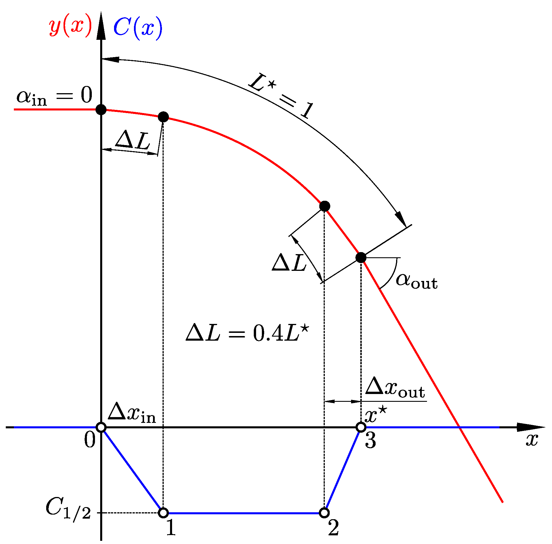
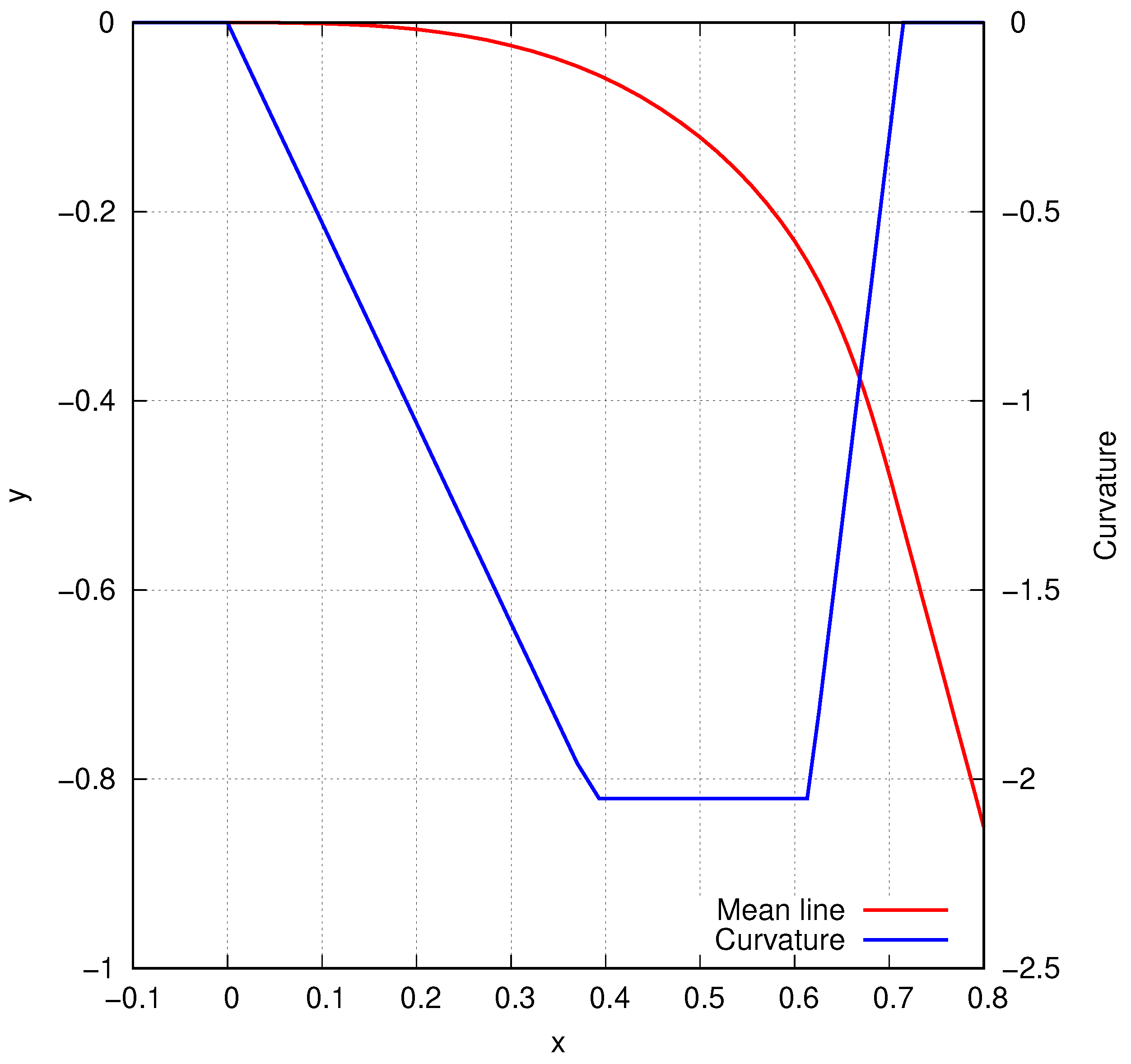
In the present study, the mean line is constructed from three main sections. The first is a straight segment extending from the upstream region to the blade-row inlet. The second is a circular arc that turns the flow from the inlet direction toward the passage throat. The third is a straight segment extending from the throat toward the blade-row outlet. To avoid abrupt changes in curvature at the junctions between the straight segments and the circular arc, short transition segments with linearly varying curvature are introduced.

The resulting mean-line geometry and corresponding curvature distribution are shown in dimensionless form in Figure 1, with the throat arc length normalized such that $L^{{\displaystyle ★}}=1$. The relationship between the prescribed curvature distribution and the resulting mean-line shape is defined by the specified-curvature method described in Appendix A. An iterative procedure is used to determine $x^{{\displaystyle ★}}$ so that the dimensionless arc length to the throat satisfies $L^{{\displaystyle ★}}=1$. During this procedure, the widths of the linear-curvature transition segments are kept constant and are defined as $\Delta x_{\mathrm{in}}=\Delta L$ and $\Delta x_{\mathrm{out}}=\Delta L/\sqrt{1+{tan}^2{\alpha }_{\mathrm{out}}}$.

3.2. Mach Number Profiles Along the Mean Line

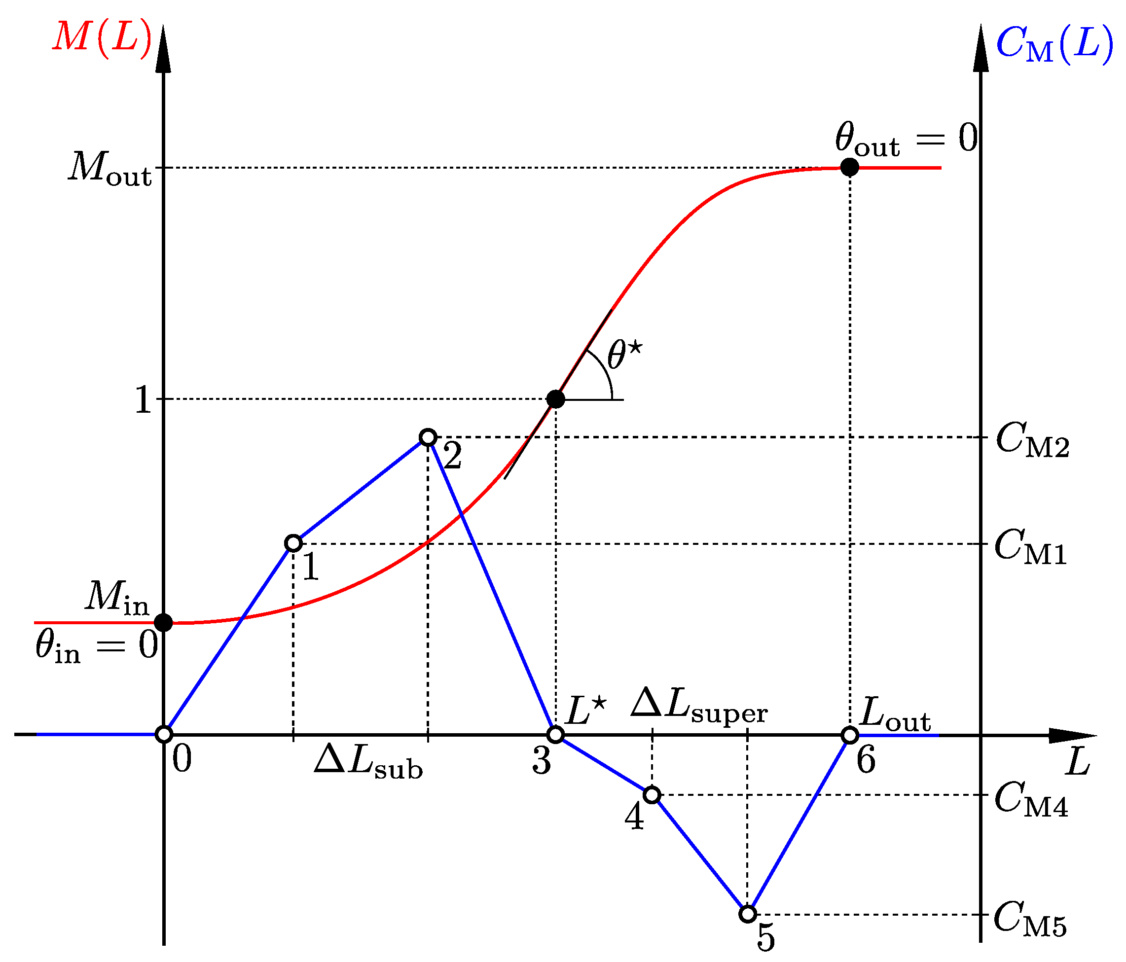
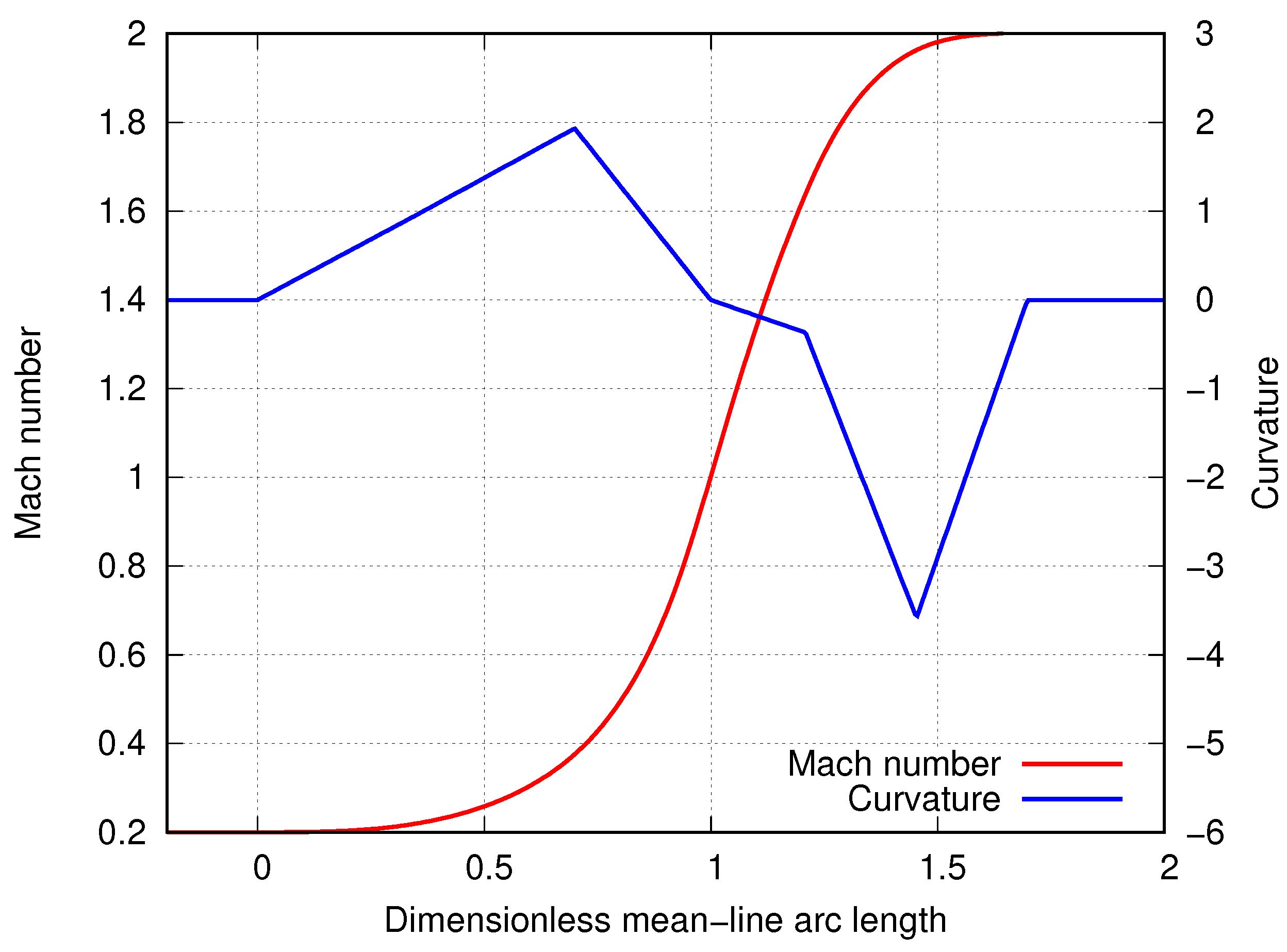
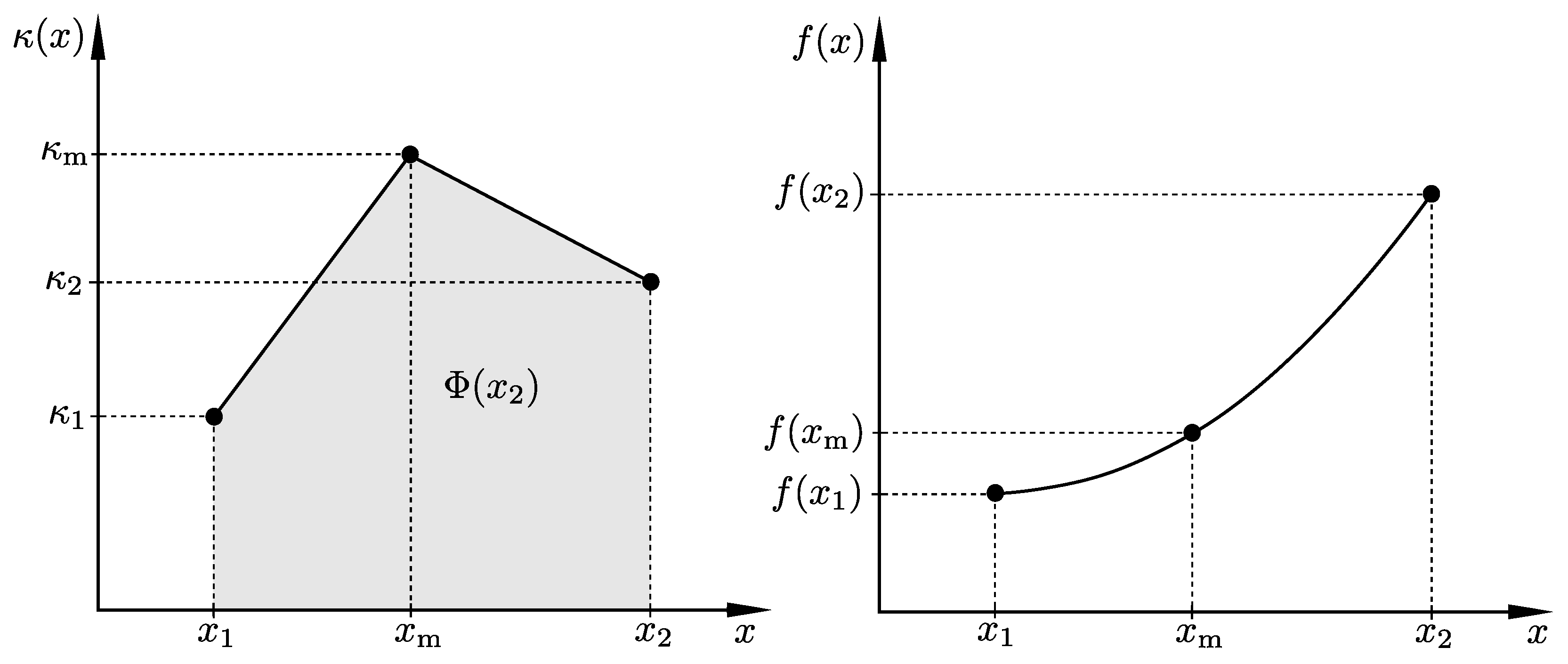
The Mach number profile along the mean line of the inter-blade passage indirectly determines the lengths of the subsonic and supersonic portions of the nozzle. In the present study, the Mach number distribution is prescribed as a function of the mean-line arc length using the specified-curvature method described in Appendix A. A representative Mach number profile, together with the corresponding curvature distribution, is shown in Figure 2. The profile is divided into subsonic and supersonic regions, which are separated by the sonic point, or throat, located at $L^{{\displaystyle ★}}$. Each region is further partitioned into three equal segments along the arc length, such that $\Delta L_{\mathrm{sub}}=L^{{\displaystyle ★}}/3$ and $\Delta L_{\mathrm{super}}=(L_{\mathrm{out}}-L^{{\displaystyle ★}})/3$. The curvatures $C_{\mathrm{M}1}$, $C_{\mathrm{M}2}$, $C_{\mathrm{M}4}$, and $C_{\mathrm{M}5}$ are determined such that the constraints given by Equations (A9) and (A10) are satisfied. The slope of the Mach number profile at the sonic point, denoted by ${\theta }^{{\displaystyle ★}}$, is optimized by minimizing the integral of the squared curvature over the subsonic and supersonic regions. Outside the interval $[0,L_{\mathrm{out}}]$, the Mach number is assumed to remain constant.

The velocity field along the mean line is computed from the specified Mach number profile under the assumption of isentropic expansion. First, the static enthalpy is obtained from the lookup table representing the relation given in Equation (10). The corresponding velocity magnitude is then evaluated using Equation (4). The velocity vector is assumed to be tangent to the mean line at each point.

3.3. Calculate Velocity Field Using PINN

In this study, the inverse design of a supersonic nozzle with a curved mean line is formulated as a physics-informed learning problem. The mean-line geometry and the tangential velocity distribution along the mean line are prescribed as defined above. A fully connected neural network (multilayer perceptron) is trained to satisfy the boundary condition along the mean line and to enforce the governing PDEs (1) and (2) in the limited regions above and below it, where the nozzle contours are expected to lie.

According to the approach described above, the solution of the PDEs is approximated by a fully connected neural network $\widehat{\mathbf{v}}\left(\mathbf{r}\right)$. For any input vector $\mathbf{r}$ representing the two-dimensional spatial coordinates, the network returns an approximation of the solution field $\mathbf{v}\left(\mathbf{r}\right)$, which in this study corresponds to the velocity vector field. Accordingly, the nonlinear approximation function $\widehat{\mathbf{v}}\left(\mathbf{r}\right)$ is organized as a sequence of $L+1$ layers. The first layer, ${\mathbf{z}}^0={\mathbf{z}}^0\left(\mathbf{r}\right)$, consists of the two spatial coordinates. Each subsequent layer ℓ is parameterized by a weight matrix ${\mathbf{w}}^{\mathcal{l}}\in {\mathbb{R}}^{d_{\mathcal{l}}\times d_{\mathcal{l}-1}}$ and a bias vector ${\mathbf{b}}^{\mathcal{l}}\in {\mathbb{R}}^{d_{\mathcal{l}}}$, where $d_{\mathcal{l}}$ denotes the output size of layer ℓ. Layers ℓ with $\mathcal{l}\in \{1,\dots ,L-1\}$ are called hidden layers, and their outputs are defined recursively as

$${\mathbf{z}}^{\mathcal{l}}=\sigma \left({\mathbf{w}}^{\mathcal{l}}{\mathbf{z}}^{\mathcal{l}-1}+{\mathbf{b}}^{\mathcal{l}}\right),\mathcal{l}=1,\dots ,L-1,$$

(11)

where $\sigma$ is the activation function, selected in this work as the hyperbolic tangent function. The last layer (output layer) represents two velocity vector components and it is defined as

$${\mathbf{z}}^L={\mathbf{w}}^L{\mathbf{z}}^{L-1}+{\mathbf{b}}^L.$$

(12)

Finally, the full neural network can be written as the composition

$$\widehat{\mathbf{v}}(\mathbf{r},\theta )=\left({\mathbf{z}}^L\circ {\mathbf{z}}^{L-1}\circ \dots \circ {\mathbf{z}}^0\right)\left(\mathbf{r}\right),$$

(13)

where ∘ denotes function composition and $\theta ={\{{\mathbf{w}}^{\mathcal{l}},{\mathbf{b}}^{\mathcal{l}}\}}_{\mathcal{l}=1}^L$ represents the trainable parameters of the network (hyperparameters).

The training of the network (13) represents determination of the hyperparameters of the network by solution of the following optimization problem:

$${\theta }^{{\displaystyle ★}}=\underset{\theta }{\mathrm{argmin}}\mathcal{L}\left(\theta \right)$$

(14)

where $\mathcal{L}\left(\theta \right)$ is the loss function consisting of supervised and unsupervised part:

$$\mathcal{L}\left(\theta \right)={\mathcal{L}}_{BC}\left(\theta \right)+{\mathcal{L}}_{PDE}\left(\theta \right).$$

(15)

The supervised component of the loss ${\mathcal{L}}_{BC}\left(\theta \right)$ is associated with points in the spatial solution domain where the target solution is known, such as points with prescribed Dirichlet boundary conditions. In contrast, the unsupervised component ${\mathcal{L}}_{PDE}\left(\theta \right)$ corresponds to the residuals of the governing PDEs evaluated at points where the solution is not known a priori. Both components of the loss function are calculated by mean square error procedure:

$${\mathcal{L}}_{\mathrm{BC}}\left(\theta \right)={\displaystyle \frac{1}{n_{DP}}}{\displaystyle \sum _{i=1}^{n_{DP}}}{|\widehat{\mathbf{v}}({\mathbf{r}}_i,\theta )-{\mathbf{v}}_i|}^2,$$

(16)

$${\mathcal{L}}_{\mathrm{PDE}}\left(\theta \right)={\displaystyle \frac{1}{n_{CP}}}{\displaystyle \sum _{i=1}^{n_{CP}}}|{\mathcal{R}}_1\left[\widehat{\mathbf{v}}({\mathbf{r}}_i,\theta )\right]{|}^2+{\displaystyle \frac{1}{n_{CP}}}{\displaystyle \sum _{i=1}^{n_{CP}}}{\left|{\mathcal{R}}_2\left[\widehat{\mathbf{v}}({\mathbf{r}}_i,\theta )\right]\right|}^2,$$

(17)

where ${\mathcal{R}}_1$ and ${\mathcal{R}}_2$ denote the residual operators corresponding to the left-hand sides of the governing partial differential Equations (1) and (2), respectively. The summations are performed over $n_{DP}$ data points and $n_{CP}$ collocation points. The collocation points (CPs) are spatial locations at which the governing equations are enforced during training; specifically, the PDE residuals are evaluated and minimized at these points as part of the loss function.

The minimization problem in Equation (14) can be solved using stochastic gradient descent (SGD) algorithms [45]. In each iteration, the hyperparameters are updated as follows:

$${\theta }^{i+1}={\theta }^i-{\eta }^i{\nabla }_{\theta }\mathcal{L}\left(\theta \right),$$

(18)

where i denotes the current iteration and $\eta$ is the learning rate. In this work, the Adam algorithm [46] is used as the stochastic gradient descent (SGD) optimizer. The gradient of the loss function is evaluated by backpropagation [47], i.e., reverse-mode automatic differentiation (AD) applied to the neural-network computational graph. In the PINN framework, AD is also used to compute the spatial derivatives of the neural-network output with respect to the input coordinates. These derivatives are then substituted into the governing differential operator to evaluate the PDE residual at the collocation points.

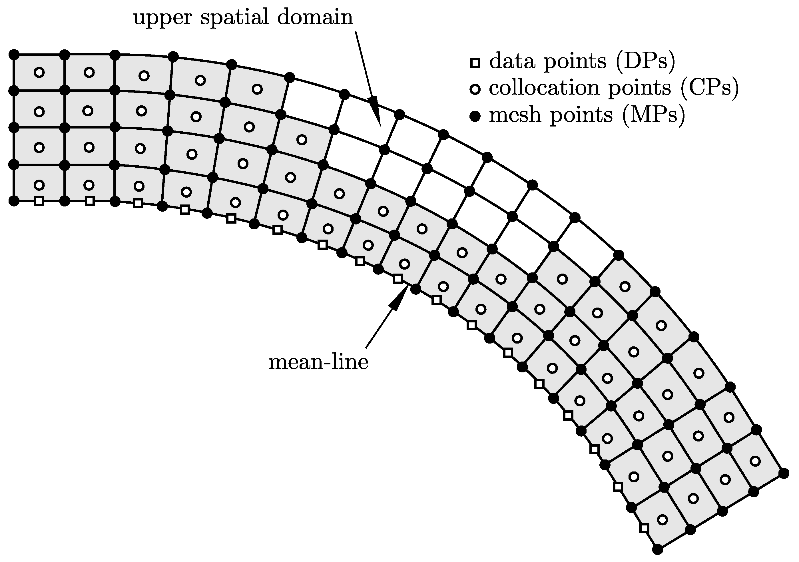
To facilitate the placement of collocation points (CPs) and training data points (DPs), quadrilateral spatial domains are constructed above and below the mean line and discretized using structured meshes. Figure 3 shows a sketch of the discretized mean line and the structured mesh in the region above it; a similar mesh is also created below the mean line. The training data points are located on the mean line, at the centres of the straight-line segments, whereas the collocation points are placed at the centres of the quadrilateral elements of the structured meshes. To reduce the number of CPs, these points are placed only in the region where the nozzle contour is expected to lie, as predicted by one-dimensional theory.

In the above described classical PINN framework, Dirichlet boundary conditions on the mean line are implemented by soft enforcement [31], where boundary prediction error is minimised through the composite loss function. In this work, boundary conditions are imposed in a hard manner by constructing the neural-network approximation so that the prescribed boundary conditions are satisfied identically, following the trial-solution approach used in neural-network-based differential equation solvers [40] and in a PINN with distance-function-based exact boundary enforcement [38]. Accordingly, the neural network approximation of the PDE solution is defined as follows:

$$\widehat{\mathbf{v}}(\mathbf{r},\theta )={\mathbf{v}}_{\mathrm{BC}}\left(\mathbf{r}\right)+D\left(\mathbf{r}\right)\tilde{\mathbf{v}}(\mathbf{r},\theta ),$$

(19)

where ${\mathbf{v}}_{\mathrm{BC}}\left(\mathbf{r}\right)$ is a particular solution, defined as a globally smooth function that satisfies the boundary conditions on the mean line. In this work, the particular solution is also represented by a fully connected neural network trained in a supervised manner using the specified velocity field along the discretized mean line. Accordingly, the loss function is defined by Equation (16). The scalar function $D\left(\mathbf{r}\right)$ represents the distance from the mean line and is defined using a pre-trained deep neural network. The approximation function given by Equation (19) is trained by optimizing the hyperparameters of the fully connected neural network $\tilde{\mathbf{v}}(\mathbf{r},\theta )$, hereafter referred to as the correction network. 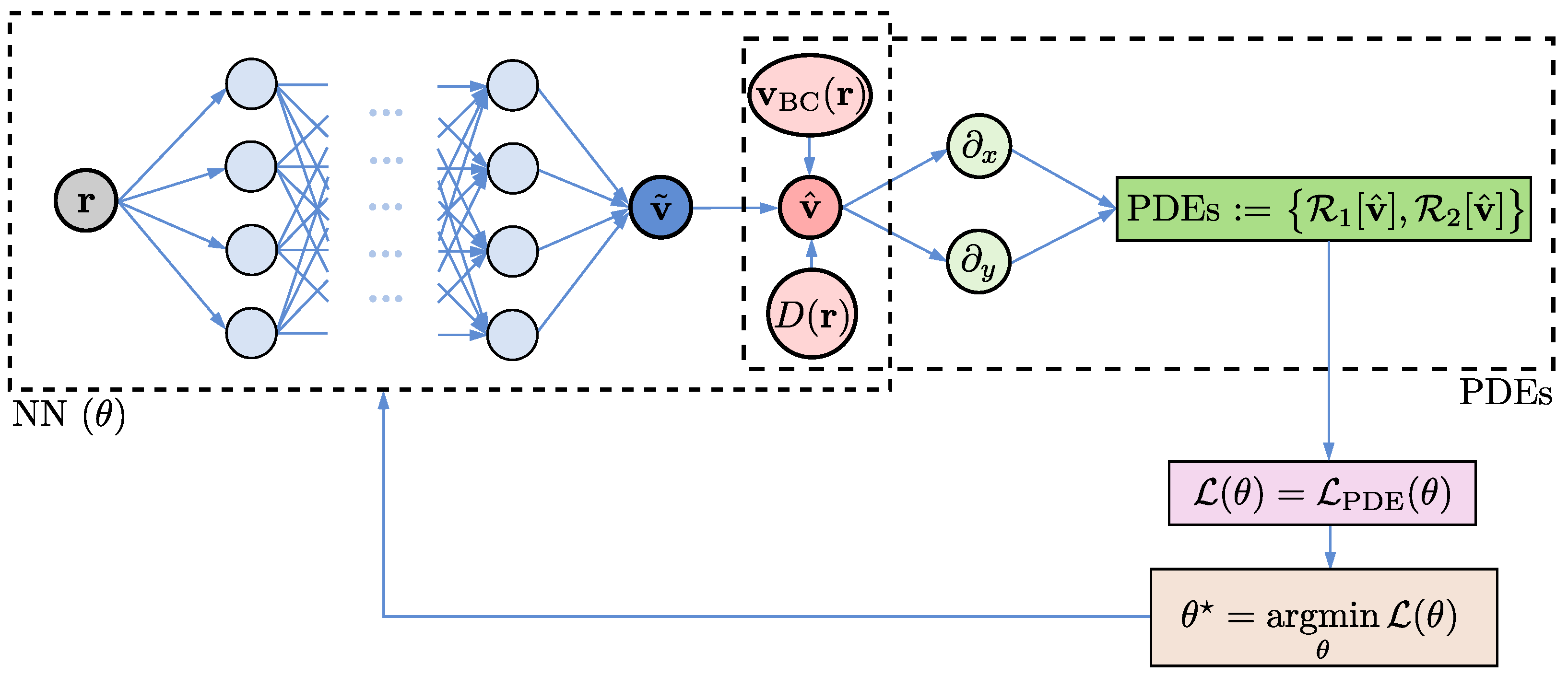The corresponding loss function contains only the PDE residual term, such that $\mathcal{L}\left(\theta \right)={\mathcal{L}}_{\mathrm{PDE}}\left(\theta \right)$, which is evaluated using Equation (17). This formulation is adopted because the particular solution already satisfies the boundary conditions along the mean line. A graphical representation of the PINN architecture is shown in Figure 4.

3.4. Stream Function Field Reconstruction

After an approximate solution of the governing PDEs is obtained using a PINN, the velocity and density are evaluated at the centres of all quadrilateral elements of the structured meshes created above and below the mean line. The stream function can then be calculated for all elements of the structured mesh using the discretized form of Equation (9). For example, the stream function at the centre of an element P adjacent to the mean line can be calculated as follows:

$$\begin{array}{cc}\hfill {\psi }_P={\psi }_{\mathrm{ml}}& -0.5\left[{\rho }_P{\left({\widehat{\mathbf{v}}}_P\right)}_y+{\rho }_{\mathrm{ml}}{\left({\widehat{\mathbf{v}}}_{\mathrm{ml}}\right)}_y\right](x_P-x_{\mathrm{ml}})\hfill \\ \hfill & +0.5\left[{\rho }_P{\left({\widehat{\mathbf{v}}}_P\right)}_x+{\rho }_{\mathrm{ml}}{\left({\widehat{\mathbf{v}}}_{\mathrm{ml}}\right)}_x\right](y_P-y_{\mathrm{ml}}),\hfill \end{array}$$

(20)

where the subscript $\mathrm{ml}$ denotes quantities evaluated at the centre of the line segment coinciding with the mean line. The stream-function value at the mean line, ${\psi }_{\mathrm{ml}}$, is set to zero. Accordingly, the stream-function values above the mean line are positive, whereas those below the mean line are negative.

After the stream-function values are computed at the element centres, the corresponding values at the mesh points are obtained by linear interpolation. The mesh-point values of the stream function are then used to reconstruct the stream-function isolines, or streamlines, which define the supersonic nozzle contours. The selected stream-function values representing the inter-blade passage contours determine the mass flow rate of the fluid through the passage.

3.5. Stator Blade Profile Reconstruction

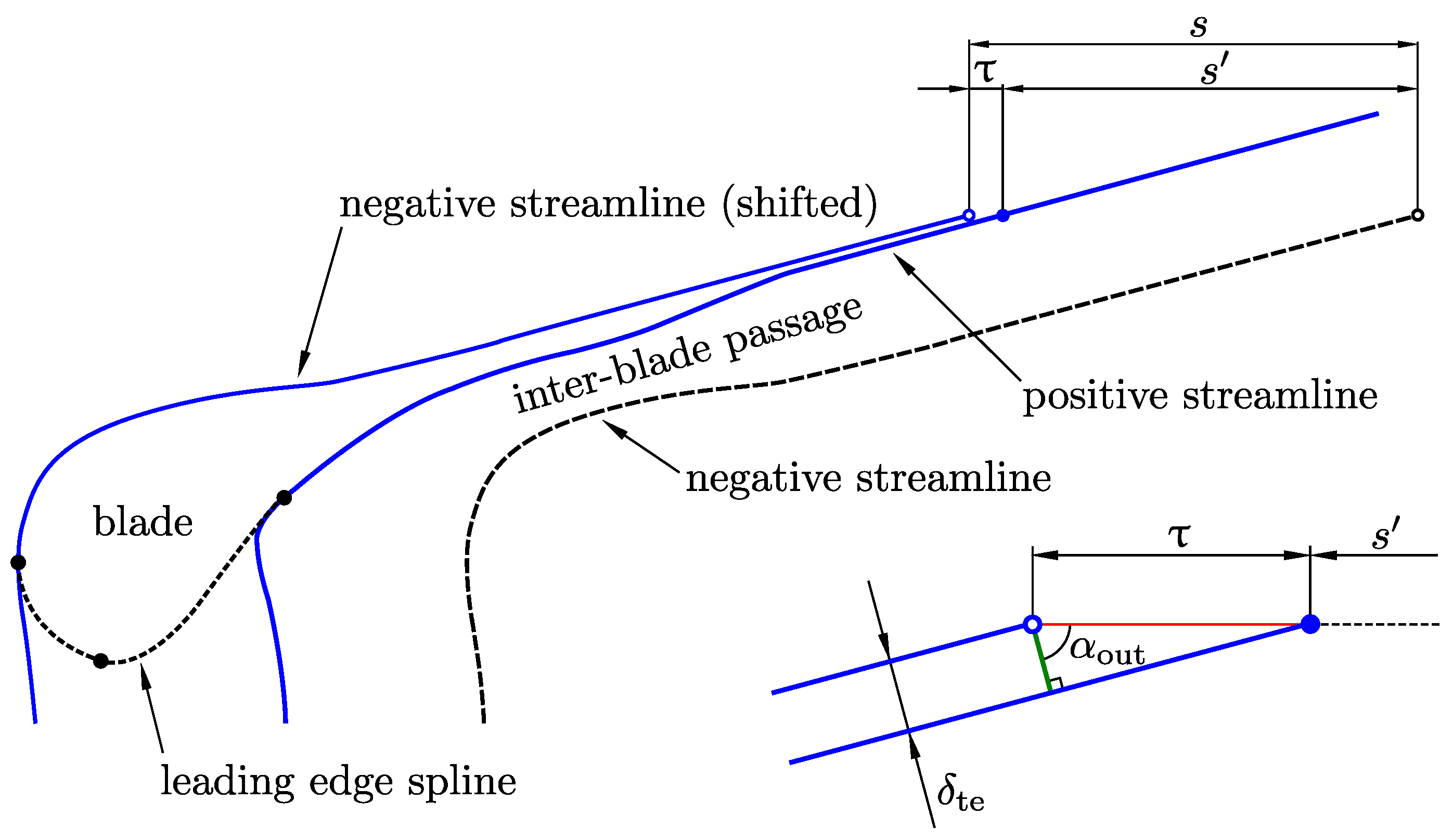
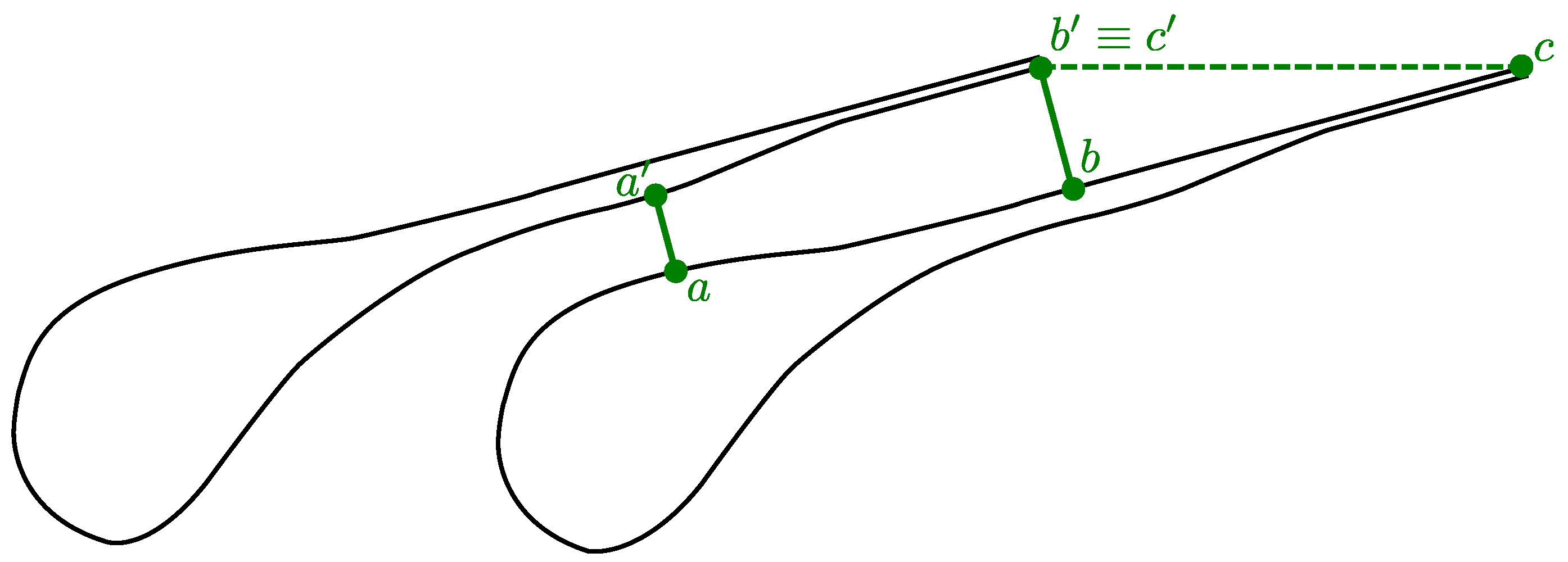
At this stage, two streamlines representing the contours of the inter-blade passage are determined. The positive streamline represents the pressure side of the stator blade, whereas the negative streamline represents the suction side. Figure 5 shows the mean line, the negative and positive streamlines, and a copy of the negative streamline shifted tangentially for the span s of the blade row. The span is determined such that the shifted negative streamline forms the required trailing-edge thickness relative to the positive streamline,

$$s=s^{\prime }+\tau =s^{\prime }+{\displaystyle \frac{{\delta }_{\mathrm{te}}}{cos{\alpha }_{\mathrm{out}}}},$$

(21)

where $s^{\prime }$ is the tangential distance between the tip of the negative streamline and the corresponding point on the positive streamline and ${\delta }_{\mathrm{te}}$ is the thickness of the trailing edge of the blade. The leading edge of the blade profile is defined by an arbitrary spline with a continuous first derivative at the joint points, and tangential position of its midpoint is obtained by minimizing the integral of the squared curvature.

3.6. Implementation of the PINN Algorithm

The proposed PINN-based inverse-design procedure is implemented by coupling a neural-network solver developed using the LibTorch 2.3.1+cpu C++ library, i.e., the C++ distribution and API of PyTorch [48], with field-manipulation utilities built on OpenFOAM-v2412 [49]. LibTorch provides the tensor operations, automatic differentiation, and C++ frontend required for training and evaluating the neural-network models, whereas OpenFOAM-v2412 provides the finite-volume data structures and field-processing capabilities used for spatial-domain discretization and flow-field manipulation. This integrated implementation supports the complete workflow within a unified C++ environment, including spatial-domain discretization, training-data preparation, neural-network optimization, and post-processing of the reconstructed velocity and stream-function fields. The overall software architecture and several implementation strategies adopted in the present PINN-based design framework were inspired to a large extent by the approach described in [50]. Final visualization and qualitative inspection of the computed fields are performed in ParaView, an open-source platform for scientific data analysis and visualization [51].

3.7. Well-Posedness of the Inverse-Design Formulation

The present method is not intended to serve as a general boundary-value solver for an arbitrarily prescribed physical domain. Instead, it is formulated as a regularized local inverse-design problem within a bounded neighborhood of a prescribed passage mean line. Because the governing equation changes type—from elliptic in the subsonic region to hyperbolic in the supersonic region—the question of existence, uniqueness, and stability of the inverse solution is particularly relevant.

In the present study, we hypothesize that, for the considered class of two-dimensional supersonic axial-turbine stator blade design problems, the prescribed mean-line geometry and velocity distribution, together with the governing-equation and the regularization introduced by the PINN formulation, are sufficient to obtain a stable and physically meaningful inverse solution. The numerical examples considered in this work support this hypothesis by producing smooth and consistent velocity fields and blade profiles. However, these numerical results do not constitute a rigorous mathematical proof of well-posedness. The conclusions are therefore restricted to the configurations and operating conditions examined in this study. A rigorous analysis of solution existence, uniqueness, and continuous dependence on the prescribed data is deferred to future work.

4. Results

The inverse-design method described above for supersonic turbine stator blades is applied to two working fluids: air, modelled as a perfect gas, and toluene undergoing transcritical expansion. The critical temperature and pressure of toluene are $T_{\mathrm{c}}=591.75\mathrm{K}$ and $P_{\mathrm{c}}=4.108\mathrm{MPa}$, respectively. The stagnation temperature and pressure of each fluid, together with the static pressure at the nozzle inlet and exit, are reported in

Table 1. Thermodynamic boundary conditions for the air and toluene nozzle-design cases.

Property	Unit	Air	Toluene
Stagnation temperature	$\mathrm{K}$	580	660
Stagnation pressure	$\mathrm{kPa}$	860	6300
Inlet pressure	$\mathrm{kPa}$	636.5	6208
Exit pressure	$\mathrm{kPa}$	0.109	0.696
Throat density	$\mathrm{kg}/{\mathrm{m}}^3$	3.275	113.97
Throat speed of sound	$\mathrm{m}/\mathrm{s}$	440.7	165.96

. For both fluids, the inlet and exit pressures are prescribed so as to obtain inlet and exit Mach numbers of approximately $0.2$ and 2, respectively.

The lookup tables for $c\left(h\right)$, $\rho \left(h\right)$, and $h\left(M\right)$ were all constructed using 200 uniformly spaced nodes over their respective independent-variable ranges. Linear interpolation is used to evaluate the tabulated quantities during PINN training. The interpolation error was assessed separately for each table. For every pair of adjacent nodes, the linearly interpolated value at the midpoint of the interval was compared with the corresponding value obtained directly from CoolProp at the same thermodynamic state. The maximum relative interpolation errors over all tested intervals were 0.0035 % for $c\left(h\right)$, 0.0058 % for $\rho \left(h\right)$, and 0.015 % for $h\left(M\right)$.

Both nozzles are designed with the same mean-line shape, with an inlet angle of ${\alpha }_{\mathrm{in}}=0°$ and an outlet angle of ${\alpha }_{\mathrm{out}}=75°$, as shown in Figure 6. They are also designed for the same Mach number profile along the mean line, as shown in Figure 7. As described earlier, both curves are defined using the specified-curvature method, and the corresponding piecewise linear curvature distributions are shown in the same figures.

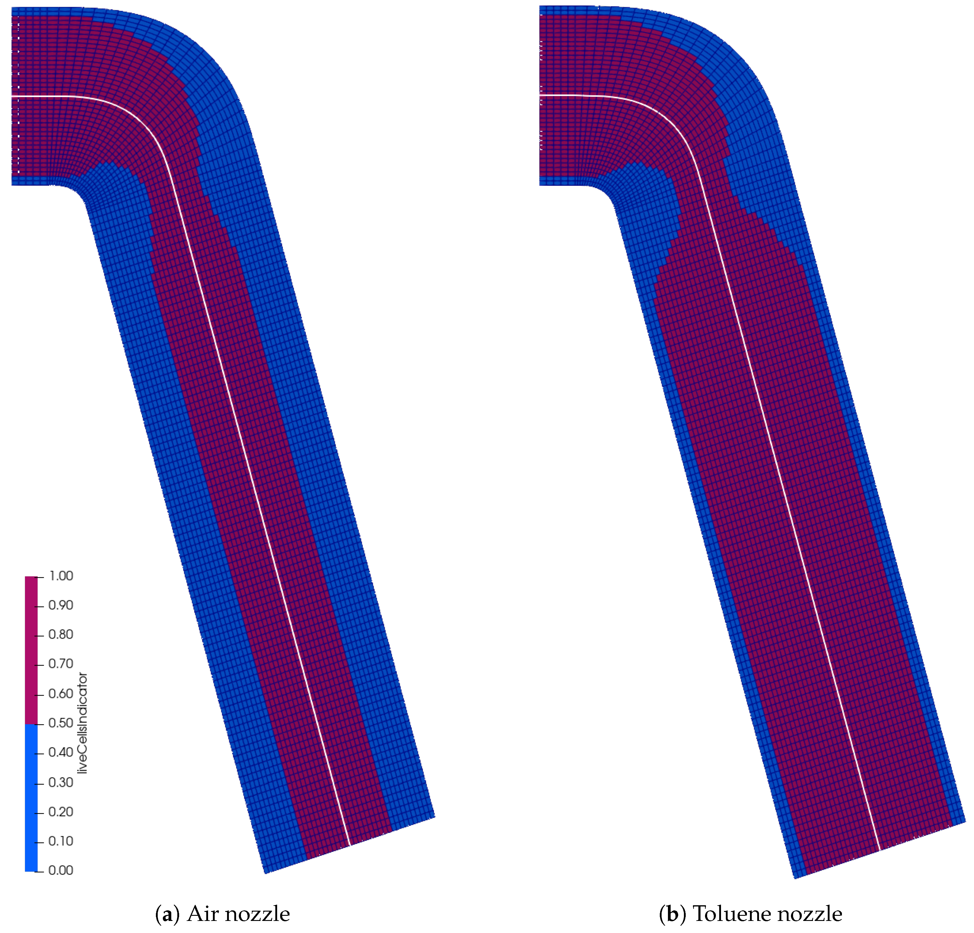
Figure 8 shows the discretized spatial domains below and above the mean line of the inter-blade passage. For clarity, a coarser discretization than the actual mesh density is shown. Active elements containing the collocation points are coloured red. The discretization includes 500 data points along the mean line, while the total number of collocation points distributed within the signed regions below and above the mean line is 10,700 for the air nozzle and 15,500 for the toluene nozzle.

The approximation of the velocity field in the vicinity of the mean line is defined by Equation (19). As described earlier, the formulation employs three artificial neural networks: the distance-function network, $D\left(\mathbf{r}\right)$; the boundary-condition network, ${\mathbf{v}}_{\mathrm{BC}}\left(\mathbf{r}\right)$; and the correction network, $\tilde{\mathbf{v}}(\mathbf{r},\theta )$. Their hidden-layer dimensions are $2\times 10$, $5\times 64$, and $5\times 128$, respectively. The distance-function network $D\left(\mathbf{r}\right)$ is trained in a supervised manner using distance data evaluated at the mean-line points and collocation points, with optimization performed using Adam. The boundary-condition network ${\mathbf{v}}_{\mathrm{BC}}\left(\mathbf{r}\right)$ is also trained in a supervised manner, using data defined at the mean-line points and the Adam optimizer. Finally, the correction network is trained using a two-stage optimization strategy that combines the Adam optimizer with the limited-memory Broyden–Fletcher–Goldfarb–Shanno (L-BFGS) method [52]. In the first stage, 2000 optimization iterations are performed using Adam with a learning rate of ${10}^{-4}$. This stage reduces the mean-squared loss to $4.0\times {10}^{-3}$ for the air nozzle and $1.6\times {10}^{-2}$ for the toluene nozzle. The resulting network parameters are then refined through an additional 150 iterations of L-BFGS optimization. Following this second stage, the mean-squared loss decreases to $3.5\times {10}^{-6}$ for the air nozzle and $5.85\times {10}^{-6}$ for the toluene nozzle.

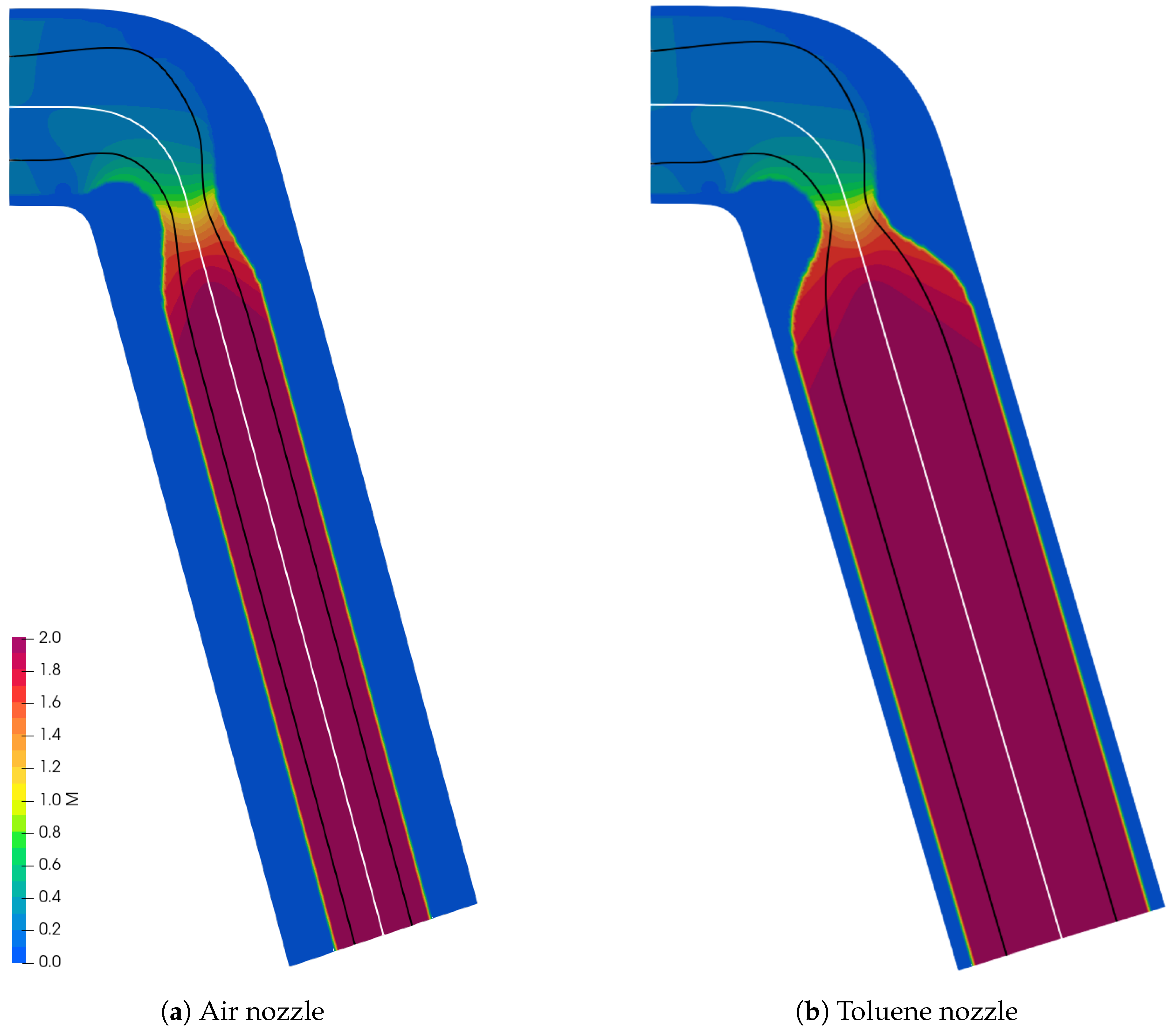
The final solutions obtained using the PINN formulation for air and toluene are shown in Figure 9. The figure presents the Mach number field in a limited region above and below the mean line, together with the positive and negative streamlines, which define the pressure and suction sides of the stator blade, respectively. The streamlines are reconstructed at dimensionless stream-function values of $\psi =\pm 0.09$ for both air and toluene. The difference between these values, $\Delta \psi =0.18$, represents both the dimensionless mass-flow rate and the dimensionless throat width. It should be noted that the stream-function values used to reconstruct the nozzle contours may be selected with some flexibility. However, these values directly influence the cascade pitch and, consequently, the required number of stator blades in the blade row. The trailing-edge thickness is not affected because it is prescribed as an input parameter, as described in Section 3.5.

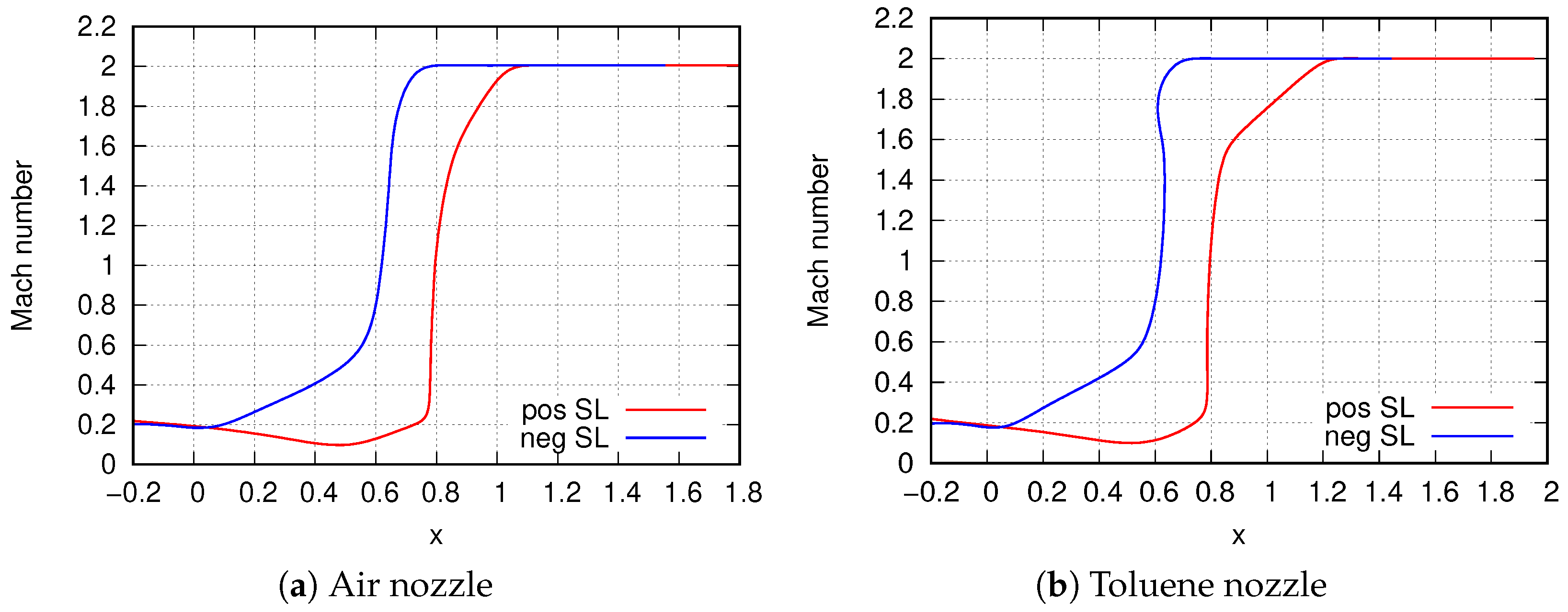
To provide the additional information required for the subsequent reconstruction of the stator blade profile, it is useful to examine the Mach number distribution along the positive and negative streamlines. This enables the required length of the supersonic part of the nozzle to be determined. The corresponding Mach number profiles are shown in Figure 10. It can be observed that, downstream of approximately $x=1.1$ for air and $x=1.3$ for toluene, the Mach numbers along the positive and negative streamlines become equal. Therefore, these axial locations are selected as the positions at which the trailing edge of the stator blade profile should end.

To verify the proposed inverse-design method, the passages defined by the positive and negative streamlines shown in Figure 9 are discretized using structured finite-volume meshes, and the inviscid flow is simulated using Ansys Fluent, Release 2025 R2 [53]. At the inlet, a pressure-inlet boundary condition is prescribed, with the stagnation pressure and temperature specified according to Table 1. At the outlet, a pressure-outlet boundary condition is used with a specified static pressure. Toluene is modelled as a real gas using the NIST real-gas model available in Ansys Fluent, with thermophysical properties based on the NIST REFPROP database [54]. The numerical solution is obtained using the density-based solver with an implicit formulation, the AUSM flux type, and third-order MUSCL spatial discretization.

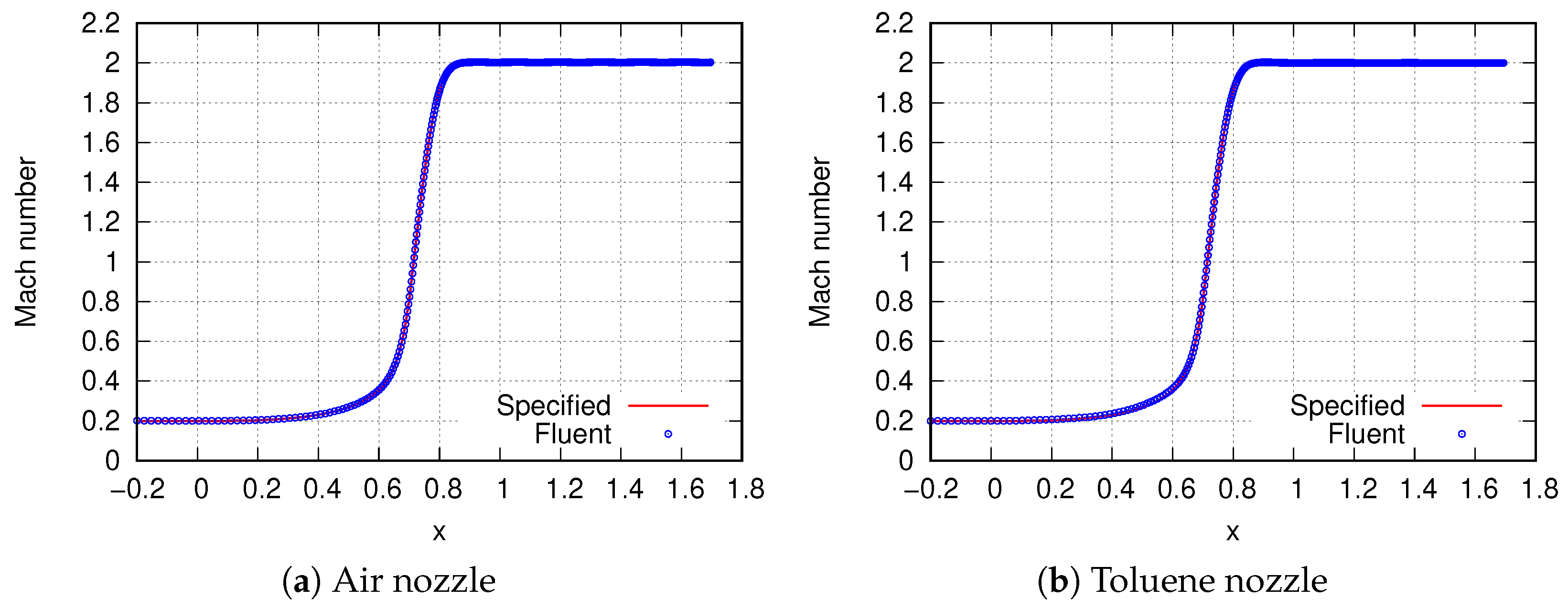
The Mach number profile along the mean line, obtained by the Ansys Fluent 2025 R2 simulation, is shown in Figure 11 for air and toluene and compared with the prescribed Mach number profile used in the inverse-design procedure. The two profiles exhibit very good agreement, confirming that the reconstructed passage accurately reproduces the target flow distribution along the mean line.

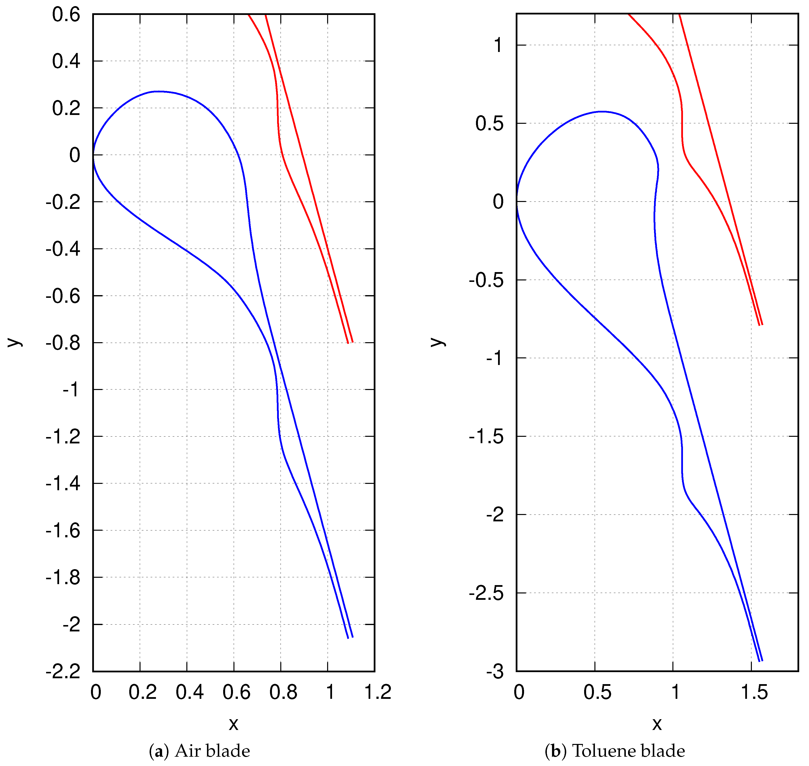
The final step of the inverse design procedure is the reconstruction of the stator blade profile from the positive and negative streamlines, following the procedure described in Section 3.5. The resulting dimensionless profile geometries for air and toluene are shown in Figure 12. In both cases, the dimensionless trailing-edge thickness is prescribed as ${\delta }_{\mathrm{te}}=0.02$. The corresponding dimensionless stator-blade cascade pitches are $s=1.256$ for air and $s=2.146$ for toluene. One should note that the dimensionless cascade pitch is an inherent parameter of the resulting dimensionless blade profile. Therefore, the pitch must be scaled by the same factor as the blade profile in order to preserve the physically consistent inter-blade passage geometry after dimensional scaling.

The dimensionless blade profiles shown in Figure 12 are used to construct two-dimensional blade cascades with a pitch of $s=11.5\mathrm{mm}$. To evaluate the aerodynamic performance of the cascades, CFD simulations of the flow through a single blade passage are performed using ANSYS Fluent. Periodic boundary conditions are applied in the pitch-wise direction to represent the blade row. The computational domain is discretized using an unstructured hexahedral mesh with inflation layers near the blade surface, ensuring an average $y^{+}$ value of approximately 2. The compressible turbulent flow is modelled using the Reynolds-averaged Navier–Stokes equations together with the k-$\omega$ SST turbulence model. The governing equations are solved in ANSYS Fluent using a density-based implicit solver, the AUSM flux scheme, and third-order MUSCL spatial discretization. A grid-sensitivity study is performed to verify that the predicted flow field and integral performance parameters are independent of the mesh resolution.

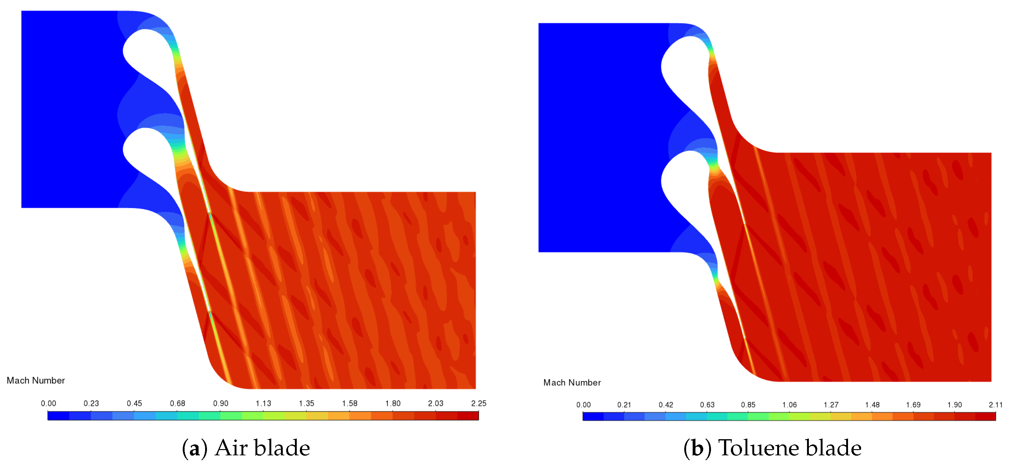
Figure 13 presents the Mach number field in the stator-blade cascade. The results reveal a smooth, shock-free flow within the inter-blade passage, with gradual acceleration governed by the blade geometry. Downstream of the trailing edge, weak fishtail shock waves emerge from both sides of the trailing edge. The corresponding performance parameters, including the dimensionless mass-flow rate, total-pressure loss coefficient, energy-loss coefficient, post-expansion ratio, and exit flow angle, are summarized in

Table 2. Aerodynamic performance parameters of the PINN-designed stator blade cascades for air and toluene, evaluated from turbulent CFD simulations.

Performance Parameter	Unit	Air	Toluene
Dimensionless mass-flow rate	1	0.178	0.177
Total pressure loss coefficient	1	0.1	0.099
Energy loss coefficient	1	0.045	0.036
Exit flow angle	°	75.07	75.15
Blade expansion ratio	1	0.253	0.212
Post-expansion ratio	1	0.957	0.989

. The associated mass-averaged exit quantities are evaluated on a plane located $4\mathrm{mm}$ downstream of the blade trailing edge. Definitions of the loss coefficients and the post-expansion ratio are provided in Appendix B.

The dimensionless mass-flow rate is very close to the reference value of $0.18$. For both fluids, the post-expansion pressure ratio is approximately unity, indicating that the stator-blade exit pressure is well matched to the downstream pressure. Consequently, the expansion is essentially completed within the blade passage, with negligible further expansion downstream of the trailing edge. This behavior is characteristic of a well-matched supersonic stator design and reduces the likelihood of post-exit expansion fans and shock-wave formation. This interpretation is further supported by the exit flow angle, which remains close to the blade metal angle and therefore indicates minimal flow deviation at the stator exit.

5. Conclusions

This paper presents a physics-informed neural-network-based design method for supersonic turbine stator blades. The proposed approach enables the generation of the complete stator-blade passage, encompassing both the converging and diverging regions, from a prescribed inter-blade-passage mean line and a target Mach number distribution along it. In contrast to conventional method-of-characteristics-based approaches, which are applicable primarily to the supersonic portion of the passage, the present method reconstructs the velocity field over the complete design region by enforcing the governing equations of steady, compressible, irrotational flow within the PINN formulation.

A hard boundary-condition strategy was adopted to impose the prescribed velocity distribution along the mean line. This was achieved by decomposing the neural-network approximation into a particular solution, a distance function, and a correction network. As a result, the prescribed mean-line velocity field is satisfied exactly, while the correction network is trained only through the residuals of the governing PDEs. Thermodynamic properties were incorporated through lookup tables for the speed of sound and density, allowing the same formulation to be applied to both ideal-gas and real-gas working fluids.

The designed passages were reconstructed from stream-function isolines obtained from the PINN-predicted velocity field. The positive and negative streamlines were used to define the pressure and suction sides of the stator blade, respectively. The method was demonstrated for two working fluids: air, treated as a perfect gas, and toluene undergoing transcritical expansion. In both cases, the inverse-designed passages reproduced the prescribed mean-line Mach number distribution with good agreement when validated by inviscid CFD simulations.

The final stator blade cascades were further assessed using turbulent CFD simulations. The computed Mach number fields showed smooth acceleration through the inter-blade passage, with no strong shock waves inside the blade channel. Weak fishtail shocks were observed downstream of the trailing edge, but the post-expansion ratio was approximately unity for both fluids, indicating that the blade-exit pressure was well matched to the downstream pressure. The exit flow angles were also close to the prescribed blade metal angle, confirming that the designed geometries achieved the intended flow direction with minimal deviation.

The results demonstrate that the proposed PINN-based design method can generate physically consistent supersonic stator blade profiles for both ideal-gas and real-gas applications. The approach reduces the reliance on heuristic prescriptions in the converging part of the nozzle and provides a flexible framework for incorporating thermodynamic real-fluid effects directly into the blade-design process.

The proposed framework may also be adapted to the design of rotor blades in impulse turbine stages. In this case, the prescribed relative-flow direction and relative Mach number distribution could be imposed along an appropriate rotor-passage mean line, while the governing equations would be formulated in the rotor-relative frame of reference. The method would also need to account for the corresponding inlet and outlet velocity triangles in order to ensure consistent matching between the stator-exit flow and the rotor-inlet conditions. Such an extension would make it possible to apply the proposed approach not only to isolated supersonic stator passages, but also to the design of complete impulse turbine stages.

Future work should focus on extending the proposed design method to three-dimensional stator blade design. In this context, the present two-dimensional formulation can serve as a basis for generating spanwise-distributed blade sections, with the prescribed mean-line geometry and Mach number profile varied along the blade span to account for radial equilibrium, end-wall constraints, and spanwise changes in loading. Such an extension would enable the reconstruction of fully three-dimensional stator geometries while retaining the main advantages of the proposed PINN-based framework, namely physics-constrained velocity-field reconstruction, direct incorporation of real-fluid thermodynamic properties, and systematic generation of blade surfaces from stream-function information. In addition, experimental validation and application to a wider range of organic working fluids and turbine operating conditions would further establish the robustness and practical applicability of the proposed method.