


Abstract
The supervisory control and data acquisition (SCADA) data are increasingly used for wind turbine anomaly detection, but purely data-driven methods may be limited by weak physical interpretability, class imbalance, and reduced generalization under changing wind-farm operating conditions. Although the Extreme Gradient Boosting (XGBoost) is effective for structured nonlinear classification, its use in SCADA-based anomaly detection remains affected by label quality, probability calibration, and cross-farm transferability. This paper validates a physics-informed XGBoost decision layer using residual-based indicators, including power-curve residuals, gearbox and generator thermal residuals, rotor-speed variance, active-power ratio, and wind-speed fluctuation. Comprehensive Anomaly Detection Benchmark for Wind Turbine SCADA Data (CARE) logbook labels are used as the reference labels, while 2σ, 3σ, and 4σ residual thresholds are evaluated as competing rule-based detectors. The decision layer is trained and internally tested using event-grouped chronological splits from Wind Farm A and externally evaluated on unseen Wind Farms B and C. The results show physically interpretable anomaly detection behavior, although performance varies across validation settings. Under external Farm A to Farm B/C transfer, XGBoost achieved row-level F1-scores of 0.6296 and 0.6551, respectively. Shapley additive explanations (SHAPs) link anomaly predictions mainly to thermal, power-conversion, and operating-context features. The findings support the proposed decision layer as an interpretable benchmark-validation framework, while showing that additional maintenance-log validation is required before definitive component-level fault-diagnosis claims can be made.
1. Introduction
Wind energy generation forms a core part of worldwide low-carbon electricity transitions [1,2]. The rapid growth of wind energy has increased the importance of operational stability, life-cycle cost management, and maintenance efficiency. In addition to installed capacity, wind farm performance is strongly affected by turbine availability, downtime, and operations and maintenance (O and M) costs [3,4]. The intermittent nature of wind generation and the maintenance requirements of wind turbines also create system-level challenges. These challenges are particularly important in emerging and fast-growing markets, where grid stability, integration costs, and unplanned outages can significantly affect the reliability and economic performance of wind energy systems [5].
Reliable wind turbine fault diagnosis is therefore essential in modern wind farms. Component failures may lead to production losses, logistical complexity, long repair times, and high safety risks [6,7]. These challenges become more significant in large-scale and geographically distributed wind farms, where maintenance activities are expensive, safety-sensitive, and operationally constrained [8]. Wind turbine diagnostic frameworks must therefore provide not only high predictive accuracy, but also reliable and interpretable outputs that can support maintenance decision-making.
Wind turbine fault diagnosis methods can generally be grouped into physics-based, data-driven, and hybrid approaches. Physics-based methods use analytical descriptions of turbine behavior based on aerodynamic, mechanical, electrical, and thermal principles. These models provide a physical interpretation of system behavior and can be used to detect abnormal operation through physically meaningful indicators such as power-curve deviations and abnormal thermal responses [6,8,9,10]. This forms the basis of residual-based fault diagnosis, where deviations between expected and observed turbine behavior are measured directly. However, physics-based methods depend on modeling assumptions and may be difficult to scale across different turbines, operating regimes, and wind farm environments [8,9,11].
Supervisory control and data acquisition (SCADA) systems have become a major source of operational data for wind turbine condition monitoring. SCADA systems provide low-cost and continuous measurements of variables such as wind speed, power output, rotor speed, component temperature, and generator-related electrical signals [6,12]. However, SCADA-based fault diagnosis remains challenging because the data may contain sensor noise, missing values, class imbalance, and variability across operating regimes [13,14,15,16]. These challenges complicate model validation because the same fault condition may appear differently under different thermal, loading, and wind conditions [12,14,15,17]. As a result, diagnostic models evaluated only using overall accuracy may produce misleading conclusions about real-world reliability [12,16,17].
Data-driven approaches use machine learning models to learn complex relationships between SCADA measurements and turbine fault states [12,15,16,17]. Machine learning (ML) and deep learning (DL) techniques can model nonlinear relationships between turbine measurements and fault classes, while deep learning architectures are particularly useful for extracting patterns from high-dimensional and time-dependent data [12,15], and [17,18,19,20,21]. Ensemble learning, convolutional architectures, recurrent models, and transformer-based methods have therefore become increasingly common in wind turbine fault detection and classification [11,18,19,20]. Convolutional architectures are useful for learning local operating patterns, while transformer-based architectures are useful for capturing long-range dependencies in temporal sequences. Nevertheless, high predictive accuracy does not always imply physically meaningful or reliable diagnostics [17,21,22,23]. Many data-driven models operate as black-box systems in which model decisions are not explicitly connected to turbine physics, limiting their practical use in maintenance decision-making [7,9,24].
Table 1 summarizes the main strengths and limitations of the three diagnostic approaches considered in this study.
Table 1.
Comparison of diagnostic approaches for wind turbine fault detection.
The limitations of purely physics-based and purely data-driven methods have motivated physics-informed and hybrid diagnostic models that use domain knowledge to guide machine learning [11,25,26]. In such approaches, structured features are constructed using physics-based or normal-behavior models, often in the form of residuals between expected and observed turbine behavior [6,10,11,27]. These residuals provide interpretable measures of abnormal operation and can be supplied to machine learning models to combine physical insight with statistical learning capability [11,17,25,26]. The usefulness of hybrid approaches, however, depends on whether physical knowledge is preserved and validated in the learning process [26].
Residual-based fault detection is therefore central to physics-informed diagnostic modeling. Power-curve residuals measure deviations between expected and measured power output at a given wind speed and can indicate aerodynamic inefficiency, drivetrain losses, or generator-related power imbalance [6,8,10]. Thermal residuals measure deviations between expected and measured component temperature behavior and are relevant to component-level degradation, including gearbox overheating and generator-related thermal imbalance [7,9]. Together, power and thermal residuals provide physically meaningful diagnostic inputs because they relate model features to expected turbine aerodynamic and thermal behavior.
The computation of power and thermal residuals is conceptually illustrated in Figure 1. The power residual is the difference between measured and expected power output at a given wind speed, while the thermal residual is the difference between measured and expected component temperature under a given operating condition. These residuals are used in this study as physics-informed input features because they measure departures from expected turbine behavior rather than relying only on raw SCADA measurements.
Figure 1.
Illustration of physics-informed residual computation: (a) power residual, the difference between measured and expected power output at a given wind speed, and (b) thermal residual, the difference between measured and predicted component temperature under a specific operating condition.
Decision-layer models such as Extreme Gradient Boosting (XGBoost) are suitable for structured residual-based feature spaces because they are effective in nonlinear classification problems and can model interactions between residual and statistical features [28,29,30]. XGBoost is a gradient-boosted decision-tree algorithm that builds an additive ensemble of decision trees to learn nonlinear relationships between input features and diagnostic labels [28,29,30]. It has been used in wind turbine fault diagnosis and reliability analysis, often together with SCADA-derived features and ensemble-learning strategies. However, the use of XGBoost does not by itself guarantee diagnostic validity. In SCADA-based wind turbine diagnosis, XGBoost-based models may still be limited by the quality of the reference labels, the possibility of learning threshold-generated decision rules rather than independent fault evidence, sensitivity to class imbalance, non-ideal probability calibration, and reduced transferability when validation is restricted to a single turbine or wind farm.
Although SCADA data, residual features, ensemble classifiers, and explainable artificial intelligence have each been used in wind turbine fault diagnosis, their combined use does not by itself establish a distinct methodological contribution. Previous studies have demonstrated the usefulness of XGBoost, random forests, hybrid XGBoost–LSTM models, adaptive thresholds, and feature-selection methods for wind turbine fault detection [28,29,30,31,32]. However, a remaining methodological issue is whether a tree-based decision layer provides diagnostic value beyond reproducing residual-threshold logic, and whether its decisions remain meaningful under event-level validation, turbine-wise transfer, farm-wise transfer, probability calibration, and physically interpretable feature attribution.
A distinction should also be made between fault diagnosis and fault-tolerant control. Fault diagnosis aims to identify abnormal operating states, whereas fault-tolerant control aims to maintain acceptable system operation after a fault has occurred. Recent studies on dual three-phase permanent magnet synchronous motor drives have proposed open-phase fault-tolerant control strategies that preserve torque capability, reduce copper losses, and maintain operation under electrical fault conditions [33,34]. Although these studies address drive-level fault-tolerant control rather than SCADA-based wind turbine anomaly detection, they are relevant because they highlight the operational value of early and interpretable fault information. The present study therefore focuses on the upstream diagnostic problem by constructing physically interpretable SCADA-derived residual features and validating an XGBoost decision layer for CARE logbook-based anomaly detection.
The XGBoost decision layer is validated under a leakage-controlled physics-informed framework for SCADA-based wind turbine anomaly detection using the CARE benchmark dataset obtained from [31]. The proposed framework uses SCADA data preprocessing, physical baseline modeling, residual and statistical feature construction, CARE logbook-based label definition, threshold-only detector baselines, supervised XGBoost classification, probability calibration, and SHAP-based interpretability analysis. The primary supervised training is conducted on Wind Farm A, where CARE logbook labels are used as the reference labels for binary normal/anomaly detection. The events are split chronologically within each class into training, validation, and testing subsets while keeping each event wholly within one split to reduce temporal leakage. The decision layer is then externally evaluated on unseen Wind Farms B and C to assess cross-farm generalization.
The remainder of this paper is organized as follows. Section 2 describes the system representation, CARE benchmark data source, physics-based performance modeling, residual generation, and feature–fault mapping. Section 3 presents the proposed diagnostic framework, including SCADA preprocessing, physics-informed feature engineering, CARE logbook label definition, threshold-based detector baselines, the XGBoost decision layer, validation metrics, and model interpretability. Section 4 presents the results and discussion, including physical-baseline reproducibility, threshold sensitivity, Farm A classifier comparison, cross-turbine and cross-farm validation, probability calibration, feature importance, and SHAP-based interpretation. Section 5 concludes the study by summarizing the main findings and the diagnostic significance of the proposed physics-informed XGBoost decision layer.
2. Physics-Informed XGBoost Decision-Layer System
In this section, the proposed physics-informed XGBoost decision-layer system for SCADA-based wind turbine anomaly detection is presented. The system architecture, the CARE benchmark data source, the feature-anomaly interpretation, the residual-generation process, the residual-based detection criterion, and the role of the XGBoost decision layer are described.
2.1. System Architecture, Data Source, and Feature-Anomaly Mapping
The proposed physics-informed XGBoost decision-layer system is shown in Figure 2. As shown in Figure 2, the proposed system consists of five main stages including the SCADA data acquisition, the data preprocessing, the physics-informed residual generation, the XGBoost-based decision-layer classification, and the interpretability and calibration assessment. The SCADA measurements are first obtained from the operation of the wind turbines. The raw measurements are then preprocessed through the data cleaning process, missing-value handling process, and the normalization process. Thereafter, physics-informed residual generation is applied to construct anomaly-relevant indicators from the power-curve residuals, the thermal residuals, and the statistical operating features. In this study, these indicators form the residual-based feature vector supplied to the XGBoost decision layer. Specifically, the vector consists of the power-curve residual, the gearbox thermal residual, the generator thermal residual, the rotor-speed variance, the active-power ratio, and the wind-speed variability. The XGBoost decision layer then classifies each SCADA observation as normal or anomalous.
Figure 2.
Workflow of the proposed physics-informed XGBoost decision-layer.
The proposed diagnostic system is based on the integration of analytical residual modeling and SCADA measurements. SCADA systems provide continuous measurements of wind turbine operating variables and are widely used in condition monitoring and predictive maintenance of wind turbines [6,12,15,27]. However, SCADA data are affected by noise, missing values, class imbalance, and variability in operating regimes, which may reduce the reliability of purely data-driven diagnostic models [12,14,16,17]. For this reason, the proposed system uses a structured feature representation in which the input features are linked to physically meaningful turbine behavior.
The data source used for validation is the CARE wind turbine benchmark dataset obtained from [31]. The CARE benchmark contains SCADA data collected from 36 wind turbines distributed across three wind farms, identified as Wind Farm A, Wind Farm B, and Wind Farm C as reported in [31]. These labels are used to distinguish the wind farm data sources within the benchmark. In this study, Wind Farm A is used for the primary supervised model development, including event-grouped chronological training, validation, and internal testing. Wind Farms B and C are then used as unseen external farms to assess cross-farm generalization. This design allows the proposed physics-informed XGBoost decision layer to be evaluated not only on held-out events from the development farm, but also under wind farm transfer conditions. The reference labels used in the supervised learning stage are obtained from the CARE records. Normal records are assigned to class 0 and anomaly records are assigned to class 1. The 2σ, 3σ, and 4σ residual-threshold criteria are evaluated as competing rule-based detector baselines against the same CARE logbook labels. The supplementary sensor harmonization and CARE event-label summaries used to support the cross-farm feature alignment are provided in Tables S1 and S3.
The feature-anomaly mapping is defined in terms of the relationship between measured SCADA variables, residual-based indicators, and turbine operating mechanisms. Power-curve residuals represent deviations between expected and measured power output and may indicate aerodynamic inefficiency, drivetrain losses, or generator-related power imbalance. Gearbox oil, generator, nacelle, and ambient temperature measurements are used to construct thermal residuals that represent abnormal heat accumulation and thermal imbalance. The residual indicators are complemented by the statistical operating features used in the proposed diagnostic system. The rotor-speed variance is used to represent changes in the rotational behavior of the turbine and provides an indication of possible drivetrain instability. The active-power ratio compares the measured power output with the expected power output at the same wind speed condition and is used to describe abnormal power-conversion behavior. The wind speed variability describes changes in the wind regime and provides the operating context required to interpret the power and thermal residuals under variable operating conditions.
The XGBoost block in Figure 2 represents the supervised machine learning decision layer of the proposed diagnostic system. In this study, the machine learning method used is Extreme Gradient Boosting, implemented as a gradient-boosted decision-tree classifier for binary normal/anomaly detection. Its role is to map the residual-based feature vector to the corresponding CARE logbook operating label.
The analytical-numerical mapping between the SCADA-derived features, the diagnostic indications, and the physical interpretations is summarized in Table 2. This mapping provides traceability between the measured variables, the residual indicators, and the turbine subsystems. It also supports the interpretability analysis presented in Section 4, where feature attribution is used to determine whether residual-based anomaly indicators influence the model’s binary CARE normal/anomaly decisions.
Table 2.
Analytical-numerical feature-anomaly interpretation mapping.
The system architecture and the feature–anomaly mapping described in this subsection provide the basis for the physics-based performance modeling presented in Section 2.2. In the next subsection, the aerodynamic and thermal relationships are used to define the expected turbine behavior from which the residual-based diagnostic indicators are derived.
2.2. Physics-Based Performance Modeling
The aerodynamic and thermal relationships that define the expected behavior of the wind turbine are presented in this subsection. These relationships establish the physical baseline against which SCADA measurements are evaluated, providing the reference required for subsequent residual generation and fault-detection analysis.
To determine a physically interpretable reference point for turbine operation, the proposed framework models wind turbine performance using aerodynamic and thermal relationships. This is consistent with physics-guided wind power modeling approaches, where physical system knowledge is combined with data-driven modeling to improve interpretability and robustness [11]. Under ideal operating conditions, the aerodynamic power, , extracted from the wind is given by:
where is the air density, is the rotor swept area, is the power coefficient, is the tip-speed ratio, is the blade pitch angle, and is the wind speed respectively. This equation defines the theoretical wind power available to the turbine and serves as a first-principle reference for aerodynamic performance.
In practice, the actual electrical power output differs from theoretical aerodynamic power because of drivetrain losses, control-system dynamics, generator conversion losses, and environmental variability [6,10,12,27]. Hence, the empirical power curve is used as the practical baseline for turbine performance because it accounts for the nonlinear relationship between wind speed and measured electrical power under actual operating conditions. The empirical power-curve baseline is represented as follows:
where is the expected turbine power output at wind speed , and is the SCADA-validated empirical power-curve function.
Under normal operating conditions, the measured SCADA power output is expected to follow the empirical power-curve relationship. Deviations from this relationship, such as reduced power production at a given wind speed, may indicate aerodynamic inefficiency, drivetrain losses, control-system abnormality, or generator-related anomalies. These deviations form the basis of the power residual, which measures the difference between expected and observed turbine behavior.
Thermal modeling is also used to represent the heat-generation behavior of critical turbine components. The temperatures measured in the gearbox, generator, and nacelle are influenced by mechanical friction, electrical loading, active power output, wind conditions, and ambient thermal effects. To establish a reference for normal thermal operation, the expected component temperature is modeled as follows:
where is the expected component temperature under normal operating conditions, is the empirical thermal baseline function learned from normal SCADA operating data, is the active power output, and is the wind speed. This expression provides a thermal baseline against which measured component temperatures can be compared.
Deviations from the expected thermal behavior are important for fault diagnosis because component degradation may appear as abnormal heating before complete failure occurs, particularly in cases of gearbox overheating and generator-related thermal imbalance [7,9].
The combination of aerodynamic and thermal modeling provides a multi-domain physical foundation for residual-based feature engineering. The aerodynamic model defines the expected power-production behavior, while the thermal model defines the expected component-temperature behavior. This formulation ensures that the derived diagnostic features retain clear physical meaning and that the model inputs can be connected to turbine operating behavior. The expected system behavior defined in this subsection is then used in Section 2.3 to generate residual features, while statistically derived thresholds are later used in Section 2.4 to distinguish between normal and abnormal operating regimes.
In the implementation used in this study, the physical baselines are fitted using healthy training-event history data only. Logged anomaly windows are excluded from the baseline fitting stage to reduce leakage between the physical model and the supervised evaluation labels. For Wind Farm A, the healthy baseline contains 125,145 rows, of which 100,114 rows are used for baseline fitting and 25,031 rows are held out for baseline validation. The healthy baseline period extends from 1 January 2022 00:00:00 to 29 August 2023 15:20:00, using status values in {0, 2}, wind speeds between 5 m/s and 10 m/s, and a trailing feature window of 12 samples, corresponding to 2 h at the 10 min SCADA sampling interval. The held-out healthy validation results show that the log-log power baseline achieved a coefficient of determination (R2) of 0.9695, a root mean square error (RMSE) of 0.0339 p.u., and a mean absolute error (MAE) of 0.0228 p.u. The lumped gearbox thermal baseline achieved an R2 of 0.7321, an RMSE of 1.5846 °C, and an MAE of 1.0031 °C, while the lumped generator thermal baseline achieved an R2 of 0.9727, an RMSE of 1.6674 °C, and an MAE of 0.9463 °C. These results provide the physical-model reproducibility information required to interpret the subsequent residual features. The detailed physical-baseline parameters, healthy-baseline windows, fit-quality metrics, and run configuration are provided in Table S2.
2.3. Residual Generation
This subsection presents the formulation of the residual and statistical features derived from the aerodynamic and thermal performance models developed in Section 2.2. These features are used to quantify deviations between expected and measured turbine behavior and constitute the diagnostic inputs to the decision layer.
Based on the physics-based performance models outlined in Section 2.2, deviations between expected and measured turbine behavior are quantified using residuals derived from SCADA measurements. These residuals transform raw operational signals into physically interpretable indicators of turbine health and form the main diagnostic feature space used by the XGBoost decision layer.
The power-curve residual is defined as follows:
where is the measured electrical power output, is obtained from the SCADA-validated power curve at wind speed and is the resulting power residual. Under normal operating conditions, this residual is expected to fluctuate around its nominal value. Sustained deviations from the expected power-curve behavior may indicate an aerodynamic inefficiency, the drivetrain losses, the control-related abnormality, or generator-related power imbalance [6,10,12,27].
Thermal residuals are used to capture abnormal heat-generation behavior in critical turbine components. The gearbox thermal residual, , is defined as follows:
where and represent the measured gearbox oil temperature and nacelle temperature, respectively. This differential formulation reduces the influence of ambient thermal variation by comparing gearbox oil temperature with nacelle temperature. Elevated values of indicate frictional losses, lubrication degradation, or bearing faults associated with gearbox overheating [7,9].
A model-based thermal residual is also expressed as:
where is the measured component temperature and is the expected component temperature under the corresponding power and wind-speed conditions and is the thermal residual. This residual separates abnormal heating effects by measuring deviations from anticipated thermal patterns.
The generator temperature gradient, , is used to describe changes in generator thermal behavior over time. It is defined as follows:
where is the generator temperature at time , and is the sampling interval. Since the SCADA records are 10 min means, corresponds to the 10 min SCADA sampling interval. High positive gradients indicate abnormal heating behavior that may be associated with generator imbalance or electrical loading [7,9].
In addition to residual features, statistical operating features are derived to describe dynamic turbine behavior. Rotor-speed variance, , is used to represent rotational instability and is defined as follows:
where is the rotor speed within a moving window, is the mean rotor speed in that window, and is the number of samples. Large values of rotor-speed variance may indicate rotational instability associated with uneven torque transfer or drivetrain disturbance.
The active-power ratio, , is used to compare measured and expected power production under the same wind-speed condition. It is defined as follows:
where is the measured active power, and is the expected power at wind speed . Values that deviate from the nominal range may indicate abnormal power-conversion behavior.
Wind-speed variability is used to account for changes in the wind regime and is defined as follows:
where is the wind speed variability at time , is the wind speed within a moving window, is the mean wind speed in that window and is the number of samples. This feature provides contextual information for interpreting power and thermal residuals under variable wind conditions.
Collectively, the residual and statistical features provide a compact representation of turbine health by linking deviations in power production, thermal behavior, rotational stability, and wind-regime variability to possible fault mechanisms. This representation improves the sensitivity of the diagnostic system to fault-related variations while maintaining a physical connection between the model inputs and the turbine operating behavior [12,15,17,21].
2.4. Residual-Based Anomaly Detection Criterion
In this subsection, the residual-threshold criterion used to identify statistically significant departures from healthy power-curve and thermal behavior is defined.
Statistical thresholding is used to transform residual signals into anomaly-relevant indicators. Under healthy operating conditions, the residuals are assumed to vary around their nominal means because of measurement noise and natural variability in turbine operation [6,12,17]. Let denote a residual signal, such as the power residual or thermal residual . The residual under healthy operating conditions is characterized by its mean, , and the standard deviation, . A statistically significant deviation is identified when:
where is the residual value at time , and is a sensitivity parameter. The parameter controls the trade-off between detection sensitivity and false-alarm rate. In this study, , , and are evaluated to determine the sensitivity of threshold-only detection to the threshold coefficient. The fixed σ thresholds are used only as transparent rule-based reference detectors and should not be interpreted as theoretically optimal anomaly limits. The use of 2σ, 3σ, and 4σ thresholds provides a sensitivity analysis of residual-threshold detection, but it does not assume that the residual distributions are strictly Gaussian or stationary across all operating regimes. SCADA residuals may vary with wind speed, turbine loading, thermal state, sensor behavior, and farm-specific operating conditions. Therefore, the threshold-only detector is used as a simple benchmark for comparison with CARE logbook labels, while adaptive, distribution-aware, or farm-specific threshold selection is treated as a future extension.
For gearbox thermal anomaly detection, the threshold is applied to the gearbox thermal residual. Taking , for instance, the criterion is defined as follows:
where is the gearbox thermal residual, is the mean gearbox thermal residual under healthy baseline conditions and is the corresponding standard deviation.
A value above this threshold indicates a statistically significant positive temperature deviation in the gearbox subsystem. This does not by itself confirm a physical fault, but it provides a fault-relevant indicator that is consistent with known degradation mechanisms such as the frictional losses, the lubrication degradation, and the bearing wear as stipulated in [7,9].
In Figure 3, the residual distributions under healthy baseline conditions, together with Gaussian approximations and three-sigma thresholds, are shown. The power residual is distributed around its nominal mean, while the gearbox thermal residual is concentrated around its healthy baseline range. The dotted threshold lines indicate the limits beyond which residual deviations are treated as statistically significant departures from expected behavior. In this validation framework, these residual-threshold criteria are used as rule-based detector baselines and sensitivity-analysis tools. The detailed label-definition and validation procedure is presented in Section 3, where CARE logbook labels are used as the reference labels for binary normal/anomaly detection.
Figure 3.
Residual distributions with Gaussian reference curves at three-sigma thresholds in physics-informed anomaly detection: (a) standardized power residual distribution, p.u. and (b) gearbox thermal residual distribution, °C at healthy baseline operating conditions.
2.5. Role of the Decision Layer
In this subsection, the XGBoost decision layer is formulated as the supervised classification component that maps the physics-informed feature vector to the CARE logbook operating label. In this paper, the term decision layer refers to the gradient-boosted decision-tree classifier that assigns each SCADA observation to either normal or anomalous operation.
The decision-layer mapping is expressed as follows:
where
In this formulation, is the trained XGBoost classification function, is the physics-informed feature vector at time , is the feature space containing the residual and statistical indicators, and is the set of operating classes where 0 and 1 represent normal operation state and anomaly state respectively. The predicted class, , belongs to one of the two CARE logbook classes. The feature vector, , includes the power-curve residual, the thermal residuals, the rotor-speed variance, the active-power ratio, and wind-speed variability.
The adopted formulation means that the classifier does not operate only on raw SCADA measurements. Instead, it uses features derived from the expected turbine behavior, allowing the classification decision to remain connected to turbine physics. This provides a more interpretable diagnostic structure than purely data-driven SCADA-based fault diagnosis methods that rely mainly on statistical correlations discussed in [21,22,28,30].
The decision layer is trained using CARE logbook labels. While thresholding provides rule-based anomaly indication, XGBoost learns nonlinear interactions between the residual and statistical features using independently defined event labels. This prevents the classifier from simply reproducing the threshold rule that generated its targets and allows the added value of the decision layer to be evaluated against threshold-only detectors and conventional machine learning baselines. The XGBoost is selected because it is suitable for structured residual-based feature spaces and supports tree-based interpretability through gain-based feature importance and Tree-SHAP analysis. This allows the decision layer to be evaluated in terms of both classification behavior and physical consistency.
3. Proposed Physics-Informed XGBoost Decision-Layer Validation Framework
This section presents the validation framework used to assess the proposed physics-informed XGBoost decision layer for SCADA-based wind turbine condition monitoring. The framework combines CARE logbook label definition, threshold-based detector baselines, XGBoost classification, probability calibration, and model interpretability analysis.
SCADA data are widely used in wind turbine fault diagnosis, but they are affected by the nonlinear, the stochastic, and noisy nature of turbine operation. Although data-driven models have shown good predictive performance, they are not always physically interpretable and may therefore be limited in operational maintenance decision-making [12,15,22]. Physics-based approaches, by contrast, provide a physical interpretation of system behavior, but they can be difficult to generalize across different operating environments and large-scale implementations [8,11]. This study addresses this limitation by validating a physics-informed XGBoost decision layer that combines residual-based feature engineering with machine-learning classification [25,26].
The framework is designed not only to evaluate predictive performance, but also to determine whether the diagnostic outputs are physically interpretable, statistically reliable, and suitable for decision support. The methodology is therefore aligned with the main objective of this study, which is to validate the XGBoost decision layer as a supervised machine learning classification component using residual-based fault indicators, classification metrics, probability calibration, and SHAP-based interpretability analysis.
3.1. Overview of the Proposed Validation Framework
The proposed validation framework follows a modular pipeline that integrates physics-informed feature construction with machine learning classification [11,25]. This section presents the methodological procedure used to evaluate whether the XGBoost decision layer is accurate, interpretable, and probabilistically reliable under event-log-based SCADA anomaly detection. The proposed physics-informed XGBoost decision-layer validation framework is shown in Figure 4.
Figure 4.
Proposed physics-informed XGBoost decision-layer validation framework.
The input to the SCADA module is the raw 10 min turbine operating record obtained from the CARE benchmark, while its output is the time-aligned SCADA measurement table containing wind speed, active power, rotor speed, thermal measurements, and other available operating variables. The input to the preprocessing module is this raw SCADA table, while its output is a cleaned and normalized dataset after missing-value handling, variable screening, and alignment with CARE event intervals. The input to the physical-baseline modeling module is the cleaned healthy training-event history, while its output is the fitted power-curve and thermal baseline models used to define expected turbine behavior. The input to the residual-generation module is the preprocessed SCADA data together with the fitted physical baselines, while its output is the physics-informed feature matrix containing power-deviation, thermal, rotor-variance, active-power-ratio, wind-fluctuation, and operating-context indicators. The input to the label-definition module is the CARE logbook file, while its output is the binary normal/anomaly reference label assigned to the corresponding SCADA records. The input to the threshold-baseline module is the residual-feature matrix and the healthy baseline residual statistics, while its output is the 2σ, 3σ, and 4σ rule-based anomaly decision used for comparison with the supervised classifiers. The input to the XGBoost decision layer is the residual-based feature matrix and the CARE logbook labels, while its output is the predicted operating label and anomaly probability. Finally, the input to the evaluation and interpretation module is the predicted label, predicted probability, true CARE label, and trained model structure, while its output consists of classification metrics, calibration curves, feature-importance rankings, and SHAP-based explanations. The detailed supporting tables for the sensor mapping, physical-baseline configuration, CARE event labels, row-level outputs, and event-level outputs are provided in Tables S1–S5.
The proposed validation framework comprises the following six successive phases:
- SCADA data acquisition and preprocessing;
- Physics-informed residual and statistical feature construction;
- CARE logbook label definition and threshold-based detector construction;
- XGBoost decision-layer training and classification;
- Model validation using classification, calibration, and generalization metrics; and
- Explainability and decision-support output using feature importance and SHAP analysis.
3.2. SCADA Data Preprocessing and Feature Matrix Construction
This subsection presents the preprocessing procedure and the construction of the feature matrix supplied to the XGBoost decision layer. The residual and statistical features defined in Section 2.3 are assembled into the input matrix used for supervised validation. After the steps that include the data cleaning, the missing-value handling, the normalization, and the alignment with CARE event intervals, each 10 min SCADA observation is represented by the feature vector below. This step reduces the influence of sensor noise, measurement uncertainty, and operating-regime variability, which are commonly reported challenges in SCADA-based wind turbine condition monitoring as shown in [6,12,27].
Let the preprocessed SCADA observation at time be represented as follows:
where is the wind speed, is the active power output, is rotor speed, is the gearbox oil temperature, is the nacelle temperature, is the generator temperature, and represents the generator-related electrical variables.
The framework is centered on physics-informed feature engineering. In this step, the expected turbine behavior defined in Section 2 is compared with measured SCADA behavior to generate residual features. Power-curve residuals represent deviations from expected aerodynamic power production, while thermal residuals represent deviations from expected component-temperature behavior. These residuals are combined with selected statistical operating features to form the structured input supplied to the decision layer [11].
The feature vector supplied to the decision layer is represented as follows:
where is the standardized power-deviation residual, is the standardized gearbox thermal residual, is the standardized generator thermal residual, is the standardized rotor-variance indicator, is the active-power ratio, is wind-speed variability, is the normalized power ramp, is the gearbox temperature gradient, is the generator temperature gradient, is the ambient–nacelle temperature difference, and is the speed–wind ratio.
This representation ensures that the decision layer is not trained only on raw SCADA measurements. Instead, the model receives a structured feature space derived from expected and observed turbine behavior. This is important because the study aims not only to classify turbine operating states, but also to determine whether physics-informed residual features provide a reliable and interpretable basis for the XGBoost decision layer.
3.3. CARE Logbook Label Definition and Threshold-Based Detector Baselines
This subsection presents the label-definition procedure and the threshold-based detector baselines used to evaluate the added value of the XGBoost decision layer. The reference labels are obtained from the CARE records. For each labeled CARE event, normal records are assigned to class 0, and anomaly records are assigned to class 1. The supervised label, , is therefore defined as follows:
This label definition means that the supervised learning problem is binary CARE logbook-based anomaly detection. The labels are not generated from residual thresholds. Instead, the CARE event records provide the reference labels against which both the threshold-only detectors and the machine-learning classifiers are evaluated.
The threshold-only detector is constructed from the residual-based criterion described in Section 2.4. For a given residual signal, , a threshold-based anomaly indication is assigned as follows:
where is the healthy baseline residual mean, is the corresponding healthy baseline standard deviation, and is the threshold coefficient. In this study, , , and are evaluated to determine the robustness of the threshold-only detector to the threshold selection.
The role of the threshold-only detector is therefore comparative. It provides a rule-based anomaly detection baseline that can be evaluated against CARE logbook labels. The XGBoost classifier is then trained using the same CARE logbook labels, rather than the threshold outputs. This separation between label definition and threshold-based detection reduces the risk that the machine learning model simply reproduces a rule that generated its own targets. The threshold-only detectors are intentionally simple and should not be interpreted as equal-capacity competitors to the supervised classifiers. Their purpose is to provide transparent residual-rule baselines against which the added value of learned nonlinear decision boundaries can be judged. The 2σ, 3σ, and 4σ thresholds are used to expose the sensitivity-specificity trade-off of residual-threshold detection under the same CARE logbook labels used to evaluate the supervised models.
3.4. XGBoost Decision Layer
This subsection presents the supervised machine learning classifier used as the XGBoost decision layer for binary wind turbine anomaly detection. In the proposed framework, XGBoost is implemented as a gradient-boosted decision-tree classifier that learns the mapping between the physics-informed SCADA-derived feature vector and the CARE logbook operating label. The model is therefore used as a classification stage within the diagnostic pipeline.
Extreme Gradient Boosting (XGBoost) is an ensemble-learning algorithm that constructs an additive model using gradient-boosted decision trees [28,29,30]. It is suitable for structured SCADA-derived feature spaces because it can learn nonlinear relationships and interactions between the residual and statistical features [25,27,30]. In the proposed pipeline, the decision layer has both a predictive and a validation role. It predicts the turbine operating label and is also used to evaluate the adequacy of the physics-informed feature representation for accurate, interpretable, and reliable anomaly detection [22].
The XGBoost model is formally represented as an additive ensemble:
where is the predicted output for sample , is the total number of trees, is the input feature vector, denotes the -th decision tree, and is a regression tree chosen from the space of possible trees .
Each subsequent tree is trained to minimize the residuals of the previous ensemble iteration by optimizing the following regularized objective function:
where is the regularized XGBoost objective function to be minimized during training and represents the set of model parameters learned by the ensemble, including the tree structures and leaf weights. The first term, is the differentiable loss function measuring the discrepancy between true labels and predictions . The second term, , penalizes the complexity of each tree.
The regularization term is expressed as follows:
where is the number of leaves, is the weight of leaf , controls the penalty for adding leaves, and controls the regularization of leaf weights. This regularization term reduces overfitting by penalizing overly complex tree structures.
For binary anomaly detection, the model estimates the anomaly probability using a logistic transformation of the model score. The predicted probability is given by:
where is the predicted probability that sample belongs to the anomaly class, is the XGBoost model score for sample . The predicted class is assigned as anomaly when and normal operation otherwise.
The binary log-loss for sample is expressed as follows:
where is the CARE logbook label and is the predicted anomaly probability.
The decision layer is trained in a physics-informed feature space, where residual-based features represent deviations between expected and measured turbine behavior. This allows the classifier to learn anomaly-relevant boundaries while retaining a direct connection to turbine operating behavior. Hyperparameter choices, including the number of trees, learning rate, and maximum tree depth, are selected to balance model complexity and generalization. However, in line with the aim of this study, hyperparameter optimization is treated as secondary to validating the decision-layer structure within the proposed physics-informed diagnostic framework. The XGBoost is therefore defined as the primary decision layer of the proposed framework before the comparative evaluation is performed. The support vector machine (SVM), random forest (RF), logistic regression (LR), and multilayer perceptron (MLP) models are included as benchmark comparators for assessing the proposed decision layer, not as alternative definitions of the framework itself.
3.5. Validation Protocol and Performance Metrics
This subsection presents the validation protocol used to evaluate the proposed physics-informed XGBoost decision layer. The model is assessed using classification performance metrics, probability calibration, cross-turbine validation, cross-farm validation, and interpretability analysis. These measures are selected because the study aims not only to evaluate classification performance, but also to determine whether the decision layer is reliable, interpretable, and physically meaningful for SCADA-based wind turbine anomaly detection.
The primary supervised training is conducted on Wind Farm A. CARE logbook labels are used as reference labels, with normal records assigned to class 0 and anomaly records assigned to class 1. Events are split chronologically within each class into 60% training, 20% validation, and 20% testing subsets, while keeping each event wholly within one split to prevent leakage across train and test sets. In the implemented Wind Farm A split, 13 events are used for training, four events are used for validation, and five events are used for testing. The physical power-curve and thermal baselines are fitted using only the training-event history data, with logged anomaly windows excluded. Model performance is first evaluated on the held-out Wind Farm A test events. Generalization is then assessed using leave-one-turbine-out validation within Wind Farm A and external Farm A to Farm B/C transfer, where the Farm A-trained classifiers are applied to target-farm residual features after target-farm physical-baseline calibration.
Several baseline approaches are included for comparison. The 2σ, 3σ, and 4σ threshold-only detectors are used to evaluate the robustness of residual-threshold diagnosis. Conventional machine learning baselines, including random forest, support vector machine, logistic regression, and multilayer perceptron classifiers, are also evaluated using the same feature representation and CARE logbook labels. This comparison is used to determine whether the XGBoost decision layer provides added value beyond threshold-only detection and standard machine learning classifiers.
The threshold-only detectors are interpreted as transparent residual-rule baselines, while the supervised classifiers are evaluated as learned decision models under event-grouped, turbine-wise, and farm-wise validation settings. Unsupervised and semi-supervised anomaly detectors, such as isolation forest, local outlier factor, and one-class SVM, are not included in the present experimental scope because they require a separate label-free or normal-only validation design. They are nevertheless important comparators for SCADA settings with scarce labeled anomalies and are identified as future work.
The overall accuracy is computed as follows:
where is the number of test samples, is the true CARE logbook label, is the predicted label, and is equal to 1 when the prediction is correct and 0 otherwise.
The balanced accuracy is also used because the number of normal and anomaly observations may be imbalanced. It is computed as follows:
precision is computed as follows:
while the recall is computed as follows:
and the F1-score is computed as follows:
where denotes true positives, denotes false positives, and denotes false negatives. Precision measures the correctness of anomaly predictions, recall measures the ability of the model to identify anomaly observations, and the F1-score provides a balanced measure of precision and recall.
The probability calibration is included because high classification accuracy does not necessarily imply reliable probability estimates. Reliability calibration curves and the Brier score are used to evaluate the predicted anomaly probabilities. The binary Brier score, , is expressed as follows:
where is the number of test samples, is the predicted anomaly probability and is the true CARE logbook label. A lower Brier score indicates better probabilistic reliability.
In addition to row-level validation, event-level validation is performed by aggregating the predicted anomaly probabilities within each CARE event. The event-level anomaly score is obtained from the upper quantile of row-level anomaly probabilities within the event. The event-level prediction is then compared with the CARE event label. This event-level assessment is important because the CARE annotations are defined at the event level and because maintenance decisions are usually made from persistent event behavior rather than isolated SCADA rows.
3.6. Model Interpretability
This subsection presents the interpretability methods used to evaluate whether the XGBoost decision layer bases its predictions on physically meaningful features. Anomaly detection in wind energy systems requires interpretability because maintenance decisions should be supported by clear and physically consistent diagnostic evidence. In the proposed framework, interpretability is therefore treated as a validation mechanism rather than an auxiliary model output.
The framework combines gain-based feature importance and Shapley additive explanations (SHAPs). Gain-based feature importance provides a global measure of how much each feature contributes to reducing the training objective through tree splits. This gives a preliminary indication of which variables are structurally important in the XGBoost ensemble [26]. SHAP provides a more detailed attribution-based interpretation by estimating the contribution of each feature to model predictions [23].
The prediction explanation for a specific sample can be written as follows:
where is the explanation model for a prediction, is the baseline model output, is the number of input features, and is the SHAP value of feature . The positive SHAP values increase the likelihood of anomaly prediction, whereas the negative SHAP values reduce it.
In this study, the SHAP analysis is applied to determine whether the XGBoost predictions are driven by physically interpretable residual and statistical features rather than arbitrary correlations in raw SCADA data. The expected outcome is that power residuals, thermal residuals, rotor-speed variance, active-power ratio, and wind-speed variability should contribute meaningfully to the model predictions because these features are physically related to turbine operating behavior and may provide diagnostic context for abnormal operation.
This relationship is important because it validates the physics-informed feature engineering process. If residual-based features appear as leading contributors to classification, it suggests that the model is using deviations from expected aerodynamic, thermal, and mechanical behavior to distinguish between normal and anomalous operating states. This strengthens both the interpretability and diagnostic validity of the proposed decision layer [25].
3.7. Decision-Support Output and Link to the Results Section
This subsection presents the final decision-support outputs produced by the proposed validation framework. The final output is a predicted operating label and its associated anomaly probability. The two operating labels are normal operation and anomaly. These outputs are supported by gain-based feature importance and SHAP analysis, which indicate how each physics-informed feature contributes to the decision process.
The framework therefore produces the following three forms of decision-support information:
- The operating-label output, which identifies whether the SCADA observation is predicted as normal or anomalous;
- The probability output, which provides a relative anomaly score whose reliability must be assessed through calibration analysis rather than interpreted directly as an absolute fault-risk estimate; and
- The interpretability output, which explains which residual-based or SCADA-derived features influenced the prediction.
Accordingly, the probability output is treated as a calibration-sensitive decision-support score. It is not assumed to be suitable for risk-based maintenance planning unless additional target-farm recalibration and maintenance-log validation are performed. This structure allows the XGBoost decision layer to be evaluated not only as a classifier, but also as a physically interpretable and probabilistically reliable decision component. The results of this validation are presented in Section 4 through classification performance, threshold sensitivity, cross-turbine and cross-farm validation, the calibration, reliability, feature importance, and SHAP-based interpretation.
4. Results and Discussion
In this section, the performance of the proposed physics-informed XGBoost decision layer is evaluated using the CARE logbook-based normal/anomaly labels. The results are presented and discussed in terms of CARE event-label structure, physical-baseline, reproducibility, threshold sensitivity, classifier comparison, cross-turbine validation, cross-farm generalization, probability calibration, feature importance, and SHAP-based interpretability.
The purpose of this section is to determine whether the XGBoost decision layer can provide an interpretable and a probabilistically meaningful anomaly detection output when trained on physics-informed residual and statistical features. Therefore, the results are interpreted as the validation of the decision layer under the CARE benchmark conditions rather than as the definitive component-level gearbox or the generator fault diagnosis.
4.1. CARE Event Labels and Data-Splitting Structure
In this subsection, the CARE event-label structure and the data-splitting strategy used for model validation are presented. This is necessary because the diagnostic labels used in the supervised learning stage are obtained from CARE event_info.csv records rather than from residual-threshold rules. The residual thresholds are therefore evaluated as detector baselines, while the CARE event records provide the reference labels used to train and test the machine learning classifiers.
For Wind Farm A, 22 CARE events are used in the supervised validation experiment. These consist of 10 normal events and 12 anomaly events. Normal records are assigned to class 0, while anomaly records are assigned to class 1. The event-label structure therefore defines a binary normal/anomaly classification task. This formulation is consistent with the objective of evaluating whether the decision layer can identify logbook-defined abnormal operating states using physics-informed residual features.
The events are split chronologically within each actual CARE class into training, validation, and testing subsets. Whole CARE events are kept within one split, so that records from the same event do not appear simultaneously in training and testing. This event-grouped splitting strategy reduces temporal leakage and provides a more realistic assessment of model performance than a randomly mixed row-level split.
Table 3 summarizes the Wind Farm A event-grouped splitting strategy. The training set contains 13 events, consisting of six normal events and seven anomaly events, with 31,536 SCADA rows from five turbines. The validation set contains four events, consisting of two normal events and two anomaly events, with 8939 SCADA rows from four turbines. The test set contains five events, consisting of two normal events and three anomaly events, with 10,096 SCADA rows from four turbines.
Table 3.
Event-grouped chronological data split for Wind Farm A.
The data structure in Table 3 shows that the validation problem is based on a limited number of labeled CARE events rather than a large number of independently verified component-failure classes. This is important for interpreting the results because row-level SCADA observations are not statistically independent when they belong to the same event. For this reason, the subsequent results are reported using both row-level and event-level indicators. The row-level metrics describe the behavior of the classifier across 10 min SCADA observations, while the event-level metrics describe the ability of the model to identify persistent logbook-defined abnormal operating periods.
The limited number of CARE events also restricts the statistical power of the event-level results. Although the row-level evaluation contains many 10 min SCADA observations, these observations are clustered within a small number of labeled events and are therefore not fully independent. Consequently, the event-level F1-score and AUC values reported in this study should be interpreted descriptively rather than as statistically definitive performance estimates. The event-level results indicate the behavior of the proposed framework under the available CARE split, but they may be sensitive to the particular event composition in the training, validation, and test subsets. Future work should evaluate larger event populations and include uncertainty quantification, such as bootstrapped confidence intervals or other event-level statistical reliability estimates, using independently verified maintenance-log labels.
4.2. Physical Baseline Training and Residual Reproducibility
In this subsection, the physical baseline used to generate the residual features is evaluated. This assessment is important because the diagnostic feature space depends on the ability of the power-curve and thermal baseline models to represent expected turbine behavior under healthy operating conditions. If the physical baselines are poorly fitted, the resulting residuals may reflect modeling error rather than abnormal turbine behavior.
The healthy baseline used for Wind Farm A is summarized in Table 4. The baseline contains 125,145 healthy SCADA rows collected from five turbines between 1 January 2022, 00:00:00, and 29 August 2023, 15:20:00. Of these records, 100,114 rows are used for baseline fitting and 25,031 rows are held out for baseline validation. The healthy baseline is defined using status values in {0, 2}, wind speeds between 5 m/s and 10 m/s, training-event histories, and exclusion of logged anomaly windows. The 10 min SCADA sampling interval is used with a trailing feature window of 12 samples, corresponding to 2 h. This baseline construction ensures that the residual features are derived from operating periods that are separated from the CARE anomaly labels used for supervised model validation.
Table 4.
Healthy baseline amount and time window for Wind Farm A.
The fit quality of the physical baseline models is presented in Table 5. The log-log power baseline achieved a coefficient of determination (R2) of 0.9619 on the fitting subset and 0.9695 on the held-out healthy subset. The corresponding held-out root mean square error (RMSE) and mean absolute error (MAE) values were 0.0339 p.u. and 0.0228 p.u., respectively. This indicates that the empirical power-curve baseline represented the healthy power-production behavior with low normalized error. Therefore, deviations from this baseline can be interpreted as power-conversion residuals rather than direct measurements of raw active-power variation.
Table 5.
Physical baseline fit quality for Wind Farm A.
The lumped gearbox thermal baseline produced lower fit quality than the power and generator thermal baselines. On the held-out healthy subset, the gearbox thermal model achieved an R2 of 0.7321, with an RMSE of 1.5846 °C and an MAE of 1.0031 °C. This result is technically reasonable because gearbox oil temperature is affected not only by active power and wind speed, but also by lubrication condition, heat retention, mechanical friction, ambient effects, and turbine-specific thermal inertia. Therefore, the gearbox residuals should be interpreted as physically meaningful thermal-deviation indicators rather than exact component-temperature predictions.
The lower gearbox thermal fit also affects the interpretation of downstream machine-learning and SHAP results. A large gearbox thermal residual may reflect genuine anomaly-associated heating, but it may also contain unexplained baseline error from thermal inertia, lubrication state, local operating history, or unmeasured component-specific effects. Therefore, this feature is treated as a moderate-confidence thermal-deviation indicator rather than a definitive gearbox-fault marker. This limitation is carried forward into the SHAP discussion, where gearbox-related attribution is interpreted as contribution to the binary CARE anomaly prediction rather than as proof of physical gearbox degradation.
To reduce the risk of over-interpreting artefactual patterns, the gearbox thermal residual is not used as standalone evidence of gearbox degradation. Instead, it is evaluated as one feature within a broader residual and operating-context feature set that also includes power-conversion, generator thermal, rotor-variance, speed–wind, and ambient–nacelle indicators. Model reliance on this feature is therefore interpreted only in combination with other physically informed features and with the calibration and external-validation results.
The lumped generator thermal baseline achieved an R2 of 0.9708 on the fitting subset and 0.9727 on the held-out healthy subset, with a held-out RMSE of 1.6674 °C and an MAE of 0.9463 °C. This indicates that the generator thermal response was represented more consistently by the selected operating variables than the gearbox thermal response. The stronger generator thermal fit suggests that generator-related thermal residuals may be less affected by unexplained baseline modeling error under the selected healthy operating range.
The physical baseline results show that the empirical power and generator thermal baselines provide strong reproducibility, while the gearbox thermal baseline provides moderate but physically interpretable fit quality. This distinction is important for the subsequent anomaly-detection results because residual magnitudes depend on both abnormal turbine behavior and the uncertainty of the physical baseline. The reported baseline sample size, time window, fitting split, and held-out error metrics therefore provide the reproducibility information needed to interpret the residual-based feature space used by threshold detectors and machine learning classifiers.
4.3. Threshold Sensitivity of Rule-Based Detectors
In this subsection, the sensitivity of the residual-threshold detector to the threshold coefficient is evaluated. This analysis is included because the use of a fixed three-sigma threshold may not be sufficient when SCADA residuals are affected by non-Gaussian behavior, changing operating regimes, sensor variability, and farm-specific operating conditions. Therefore, the threshold-only detector is evaluated at k = 2, k = 3, and k = 4 using the CARE logbook labels as the reference labels.
Table 6 presents the threshold sensitivity results for Wind Farm A, external Wind Farm B, and external Wind Farm C. In Wind Farm A, increasing the threshold coefficient from 2σ to 4σ increased row-level precision from 0.4641 to 0.6322, but reduced row-level recall from 0.1918 to 0.0531. This result shows the expected sensitivity-specificity trade-off as follows: a lower threshold detects more anomaly rows but produces more false alarms, while a higher threshold is more conservative but misses more anomaly rows. At the event level, the 2σ and 3σ detectors produced the same event F1-score of 0.7500, while the 4σ detector increased event-balanced accuracy to 0.6667 but reduced event F1-score to 0.5000.
Table 6.
Threshold sensitivity of rule-based residual detectors across Wind Farms A, B, and C.
Concerning the external Wind Farm B, the same trade-off is observed. The 2σ detector achieved the highest row-level recall of 0.3724, while the 4σ detector achieved the highest row-level precision of 0.6298 and the highest event-balanced accuracy of 0.5556. This indicates that the more conservative threshold reduced false-positive behavior at the event level, but it also reduced row-level anomaly sensitivity. The event F1-score increased from 0.5714 at 2σ and 3σ to 0.6000 at 4σ.
For external Wind Farm C, the threshold behavior was different from Wind Farm A and Wind Farm B. The 3σ detector produced the highest event F1-score of 0.6750, while the 4σ detector produced the highest event balanced accuracy of 0.5920. At the row level, the balanced accuracy values remained close across the three threshold settings, ranging from 0.5602 to 0.5614. However, row-level recall decreased from 0.3689 at 2σ to 0.2788 at 4σ, while row-level precision increased from 0.5896 to 0.6319. This confirms that the threshold coefficient controls the balance between anomaly sensitivity and false-alarm reduction.
In Figure 5, the threshold sensitivity analysis shows that residual-threshold diagnosis is physically interpretable but strongly dependent on the selected threshold coefficient and wind-farm operating distribution. Because SCADA residuals may be non-Gaussian, non-stationary, and farm-dependent, fixed global σ thresholds can be overly sensitive in some regimes and overly conservative in others. These findings support the use of threshold-only detection as a transparent baseline while motivating learned decision-layer models and future adaptive or farm-specific thresholding.
Figure 5.
Threshold sensitivity of rule-based residual detectors using 2σ, 3σ, and 4σ thresholds: (a) Wind Farm A, (b) external Wind Farm B, and (c) external Wind Farm C.
4.4. Farm-A Internal Classifier Comparison
In this subsection, the internal Wind Farm A test performance of the proposed XGBoost decision layer is compared with the threshold-only detector and conventional machine learning baselines. The comparison includes random forest, support vector machine, logistic regression, and multilayer perceptron classifiers. All machine learning models are trained using the same physics-informed feature representation and the same CARE logbook normal/anomaly labels. This comparison is important because the added value of the XGBoost decision layer should be evaluated against both simple residual-threshold diagnosis and standard supervised classifiers.
Table 7 presents the row-level and event-level performance obtained on the held-out Wind Farm A test set. The threshold-only detector achieved a row-level balanced accuracy of 0.5070 and a row-level F1-score of 0.1752. This indicates that the rule-based residual threshold provides a transparent anomaly indication, but its row-level anomaly recall is limited. The XGBoost decision layer achieved a row-level F1-score of 0.3871 and a Brier score of 0.3578. This represents a higher row-level F1-score than the threshold-only detector, showing that the supervised decision layer can extract additional anomaly relevant information from the residual and operating-context features.
Table 7.
Internal Wind Farm A classifier comparison using CARE logbook normal/anomaly labels.
Among the compared classifiers, the support vector machine (SVM) baseline achieved the highest row-level balanced accuracy of 0.5705, the highest row-level F1-score of 0.5535, the lowest row-level Brier score of 0.2439, and the highest row-level Area Under the Receiver Operating Characteristic Curve (AUC) of 0.5937. This result shows that XGBoost is not the universally best-performing classifier on the held-out Wind Farm A test set. Therefore, the contribution of the proposed decision layer is not interpreted as unconditional superiority over all machine learning baselines. Instead, the XGBoost model is evaluated as a tree-based decision layer whose classification behavior can be compared with other classifiers and interpreted through gain-based feature importance and SHAP analysis.
The event-level results show that the threshold-only detector, XGBoost, random forest, SVM, logistic regression, and multilayer perceptron (MLP) all achieved an event F1-score of 0.7500. However, the event AUC values differed across models. The SVM classifier achieved the highest event AUC of 0.6667, while XGBoost, random forest, the threshold-only detector, and MLP produced event AUC values of 0.5000. Logistic regression produced an event AUC of 0.3333. This indicates that event-level aggregation improves the persistence-based anomaly decision, but the limited number of held-out CARE test events restricts the stability of event-level ranking metrics.
Figure 6 presents the row-level confusion matrix for the XGBoost decision layer on the Wind Farm A test set. The confusion matrix shows that XGBoost identifies both normal and anomaly observations, but with substantial overlap between the two classes. This behavior is consistent with the row-level balanced accuracy of 0.4324 reported in Table 7. The result indicates that anomaly detection from 10 min SCADA observations remains challenging when normal and anomalous event windows contain overlapping operating regimes.
Figure 6.
Row-level confusion matrix for the XGBoost decision layer on the held-out Wind Farm A test set.
Figure 7 presents the row-level precision–recall curves for the threshold-only detector and the supervised machine learning classifiers. The precision–recall behavior confirms that the held-out Farm A test set is not a near-perfect separability problem. The SVM baseline shows the strongest row-level discrimination among the compared classifiers, while XGBoost provides improved anomaly F1-score relative to the threshold-only detector. This comparison is important because it demonstrates that the proposed decision-layer evaluation is not based only on XGBoost in isolation, but on a direct comparison with simple and conventional baseline methods.
Figure 7.
Row-level precision–recall curves for the threshold-only detector and supervised machine learning classifiers on the held-out Wind Farm A test set.
Figure 8 presents the row-level reliability calibration curves for the compared classifiers on the Wind Farm A test set. The calibration results show that the predicted anomaly probabilities are not perfectly calibrated across all probability intervals. The XGBoost Brier score of 0.3578 indicates moderate probability error, while the SVM baseline obtained the lowest Brier score of 0.2439. This confirms that probability calibration is an important part of the validation procedure and that classification performance should not be interpreted from accuracy or F1-score alone.
Figure 8.
Row-level reliability calibration curves for the threshold-only detector and supervised machine learning classifiers on the held-out Wind Farm A test set.
The internal Farm A comparison also clarifies the role of the SVM baseline in this study. The SVM result demonstrates that the physics-informed residual-feature representation can support stronger internal row-level discrimination than that achieved by XGBoost on the held-out Farm A test events. However, internal Farm A performance alone is not used as the sole criterion for selecting the primary decision layer. The objective of the proposed framework is to evaluate a decision layer that is not only predictive, but also interpretable and assessable under turbine-wise and farm-wise transfer conditions. For this reason, the SVM result is treated as an important internal benchmark rather than as a replacement for the XGBoost decision-layer analysis.
The XGBoost is retained because it is a tree-based decision layer that supports gain-based feature importance and Tree-SHAP interpretation, allowing the anomaly predictions to be traced to residual, thermal, power-conversion, and operating-context features. This property is central to the aim of validating whether the physics-informed feature space produces physically meaningful decision behavior. By contrast, the SVM baseline provides a strong margin-based comparator, but it does not provide the same direct tree-structured feature attribution framework used in the proposed validation pipeline.
4.5. Cross-Turbine Validation Within Wind Farm A
In this subsection, cross-turbine validation is used to evaluate whether the XGBoost decision layer can transfer across different turbines within Wind Farm A. This analysis is important because wind turbines operating in the same wind farm may still experience different local wind conditions, loading histories, sensor behavior, and thermal operating patterns. A model that performs well only on turbines represented in the training set may therefore have limited usefulness for wind-farm-level condition monitoring.
The leave-one-turbine-out validation results are presented in Table 8. In this experiment, one turbine is held out for testing while the remaining eligible turbines are used for training. The procedure is repeated across the available turbines with sufficient labeled CARE event data. The results are reported using row-level and event-level metrics to evaluate both 10 min SCADA observation behavior and persistent event-level anomaly detection.
Table 8.
Leave-one-turbine-out validation results for Wind Farm A.
As shown in Table 8, the cross-turbine results vary across the held-out turbines. The strongest row-level performance is obtained for turbine 0, with a balanced accuracy of 0.6423, an F1-score of 0.5996, and an AUC of 0.6919. Turbine 21 also shows comparatively strong transfer performance, with a row-level balanced accuracy of 0.6268, an F1-score of 0.6153, and an AUC of 0.6931. These results indicate that the decision layer can transfer useful anomaly-detection information to some unseen turbines within the same wind farm.
However, the performance is lower for turbines 11 and 13. For turbine 13, the row-level balanced accuracy is 0.5041 and the AUC is 0.5170, which indicates limited discrimination between normal and anomaly records at the row level. This variation suggests that turbine-specific operating patterns influence the residual-feature distribution and the resulting decision boundary. Such behavior is technically reasonable because residual features are affected by turbine-specific thermal inertia, local wind exposure, operating history, sensor response, and the composition of labeled CARE events available for training.
The event-level results show stronger persistence-based anomaly behavior than some of the row-level results. Event AUC values reach 1.0000 for turbines 0, 10, 11, and 21, while turbine 13 obtains an event AUC of 0.7500. Nevertheless, these event-level results should be interpreted cautiously because the number of labeled events per held-out turbine is limited. The event-level metrics indicate whether the model ranks persistent abnormal periods correctly, but they may be sensitive to the small number of available CARE events.
The leave-one-turbine-out results show that the proposed decision layer has partial cross-turbine transfer capability within Wind Farm A. The model transfers more effectively to some turbines than others, indicating that turbine-specific operating regimes remain important. This supports the need to evaluate the model not only on random row-level splits, but also under turbine-wise and farm-wise validation settings.
4.6. Cross-Farm Generalization: Farm A to Wind Farms B and C
In this subsection, cross-farm validation is used to evaluate whether the decision-layer models trained on Wind Farm A can transfer to unseen wind farms. This analysis is important because SCADA-based anomaly detection models may be affected by changes in turbine population, sensor availability, operating regime, environmental conditions, and farm-specific data distributions. Therefore, validation on Wind Farms B and C provides a stronger assessment of generalization than internal testing on Wind Farm A alone.
For the cross-farm experiment, the supervised classifiers are trained using Wind Farm A CARE logbook label and then evaluated on Wind Farms B and C. The CARE logbook labels from the target farms are used only for evaluation. Before applying the Farm-A-trained classifiers, target-farm physical baselines are fitted to construct the residual and operating-context features for each external farm. This allows the decision layer to be tested under wind-farm transfer conditions while preserving the physics-informed feature representation.
Table 9 presents the row-level and event-level cross-farm classifier comparison. For external Wind Farm B, XGBoost achieved a row-level balanced accuracy of 0.5179, a row-level F1-score of 0.6296, a Brier score of 0.3111, and a row-level AUC of 0.5504. Compared with the threshold-only detector, which achieved a row-level F1-score of 0.4062, XGBoost provided a higher anomaly F1-score. However, the random forest, logistic regression, and multilayer perceptron classifiers achieved slightly higher row-level F1-scores than XGBoost on Wind Farm B. This indicates that XGBoost transfers useful anomaly-detection information to Wind Farm B, but it is not the strongest classifier on every metric.
Table 9.
Cross-farm classifier comparison for Farm-A-trained models evaluated on external Wind Farms B and C.
For external Wind Farm C, XGBoost achieved a row-level balanced accuracy of 0.5077, a row-level F1-score of 0.6551, a Brier score of 0.4028, and a row-level AUC of 0.5679. The threshold-only detector achieved a row-level F1-score of 0.4206 and a row-level AUC of 0.5607. Therefore, XGBoost improved row-level anomaly F1-score relative to threshold-only detection, but the balanced accuracy remained close to 0.5. This shows that cross-farm transfer improves anomaly identification in terms of F1-score, while still showing limited separation between normal and anomaly rows under farm-shift conditions.
The external-farm results show that the transfer behavior is moderate and farm-dependent. In both Wind Farms B and C, XGBoost achieved higher row-level F1-scores than the threshold-only detector, which suggests that the supervised decision layer captures useful nonlinear combinations of residual and operating-context features. However, the row-level balanced accuracy values remained close to 0.5, showing that normal and anomaly records are not cleanly separated under external farm conditions. Therefore, the cross-farm results are interpreted as moderate anomaly-recovery behavior in terms of F1-score and recall, not as evidence of strong overall class separability or robust deployment-ready generalization. This result is consistent with the expected difficulty of cross-farm SCADA anomaly detection, where changes in sensor distributions, turbine operation, and farm-specific environmental conditions may shift the feature space. The supporting row-level and event-level prediction outputs used for the external cross-farm validation are provided in Tables S4 and S5, respectively.
The external-farm results also clarify the rationale for retaining XGBoost as the primary decision layer. Although the SVM baseline achieved the strongest internal Wind Farm A performance, its external-farm anomaly-detection behavior was unstable. On Wind Farm B, SVM produced very low anomaly recall and F1-score, while on Wind Farm C its row-level precision, recall, and F1-score collapsed to zero. This suggests that the SVM decision boundary learned from Wind Farm A did not transfer reliably under farm-shift conditions. By contrast, XGBoost retained useful anomaly-detection behavior on both external farms, particularly in terms of row-level recall and F1-score. Therefore, XGBoost is not presented as a universally superior classifier, but as the more appropriate primary decision layer for this study because it combines external transfer utility with gain-based and SHAP-based interpretability.
Figure 9 presents the row-level precision–recall curves for the external-farm classifier comparison. The curves show that external transfer does not produce near-perfect anomaly separation. Instead, the models show different precision–recall trade-offs across Wind Farms B and C. In Wind Farm B, the multilayer perceptron and logistic regression models achieved the highest row-level F1-scores, while XGBoost remained competitive and outperformed the threshold-only detector. In Wind Farm C, XGBoost and random forest achieved similar row-level F1-scores, with random forest producing the highest row-level AUC. These results show that the XGBoost decision layer should be interpreted as an interpretable residual-feature classifier rather than as a universally dominant classifier across all farms.
Figure 9.
Row-level precision–recall curves for Farm-A-trained classifiers evaluated on external farms: (a) Wind Farm B and (b) Wind Farm C.
Figure 10 presents the reliability calibration curves for the external-farm classifier comparison. The calibration behavior shows that probability reliability is affected by cross-farm transfer. For XGBoost, the row-level Brier score was 0.3111 on Wind Farm B and 0.4028 on Wind Farm C. These values indicate moderate probability error, especially under external-farm evaluation. Therefore, the anomaly probabilities should be interpreted together with calibration behavior and not only with the predicted class label.
Figure 10.
Row-level reliability calibration curves for Farm-A-trained classifiers evaluated on external farms: (a) Wind Farm B and (b) Wind Farm C.
The cross-farm validation results show that the proposed physics-informed feature representation and XGBoost decision layer retain useful anomaly-detection behavior on unseen farms, particularly in terms of row-level F1-score relative to threshold-only detection. However, moderate balanced accuracy and non-ideal calibration show that farm-shift effects remain important. These results support the need for external-farm validation in SCADA-based anomaly detection and suggest that target-farm calibration, domain adaptation, or farm-specific threshold adjustment may be required before operational deployment.
4.7. Probability Calibration and Reliability Across Validation Settings
In this subsection, the probability reliability of the XGBoost decision layer is discussed across the internal and external validation settings. Probability calibration is important because an anomaly-detection model should not only assign a binary operating label but should also provide probability estimates that are consistent with the observed event outcomes. This is particularly important in wind turbine condition monitoring, where maintenance decisions may depend on the confidence associated with an anomaly indication.
The reliability calibration curves presented in Figure 8 and Figure 10 show that the predicted anomaly probabilities are not perfectly calibrated across all validation settings. On the held-out Wind Farm A test set, the XGBoost decision layer obtained a row-level Brier score of 0.3578. Under external Farm-A-to-Farm-B transfer, the XGBoost Brier score was 0.3111, while under Farm-A-to-Farm-C transfer, the Brier score increased to 0.4028. These values indicate moderate probability error and show that the model probabilities should be interpreted together with the calibration curves rather than from the predicted class label alone.
Table 10 summarizes the XGBoost calibration behavior across the three validation settings. The results show that calibration reliability is affected by both the internal data split and the external wind-farm transfer condition. Although the Wind Farm B Brier score is lower than the Wind Farm A and Wind Farm C values, the cross-farm validation results still show that farm-specific operating distributions influence the relationship between predicted anomaly probability and observed anomaly frequency.
Table 10.
XGBoost probability calibration summary across validation settings.
The calibration results show that probability reliability should be evaluated separately from classification performance. Although the XGBoost row-level F1-score increased under external Farm B and Farm C testing relative to the held-out Wind Farm A test set, the Brier scores indicate that the predicted probabilities are not uniformly reliable. This behavior is technically reasonable because normal and anomalous records may overlap in residual-feature space, while external farms may differ in turbine population, sensor distributions, environmental conditions, and operating histories. Therefore, the anomaly probabilities should be interpreted as relative decision-support scores rather than calibrated probabilities of component failure. Operational use would require target-farm recalibration, adaptive calibration, or domain-adaptation procedures using additional target-farm history and independently verified maintenance records.
This distinction is important for maintenance decision-making. A high anomaly probability may be useful for prioritizing inspection, ranking event severity, or identifying persistent abnormal operating periods, but it should not be used directly as a calibrated probability of component failure or as a standalone basis for risk-based maintenance planning. Operational deployment would require target-farm probability recalibration, adaptive calibration, or domain-adaptation procedures using additional target-farm history and independently verified maintenance records.
4.8. Feature Importance and SHAP-Based Interpretation
This subsection interprets the trained XGBoost decision layer using the gain-based importance and Tree-SHAP outputs defined in Section 3.6. The focus here is on whether the learned anomaly decisions are associated with thermal, power-conversion, and operating-context feature groups, rather than on redefining the interpretability methods.
In Figure 11 the gain-based feature importance ranking of the XGBoost decision layer is presented. In this analysis, a higher gain value indicates that a feature contributes more strongly to reducing the classification loss when it is used in boosted-tree splits. The most important feature is the ambient–nacelle temperature difference, with a gain value of 52.4610. This indicates that the thermal relationship between ambient and nacelle conditions plays an important role in partitioning normal and anomalous operating regions. This result is technically meaningful because the nacelle thermal environment affects the interpretation of component-temperature behavior and can influence how thermal residuals appear under different operating conditions.
Figure 11.
Gain-based feature importance of the XGBoost decision layer for CARE logbook-based anomaly detection.
The second most important feature is the active-power ratio, with a gain value of 30.8130. This feature compares measured active power with expected power output and therefore provides a normalized representation of power-conversion consistency. Its high-ranking shows that the model uses deviations in power-production behavior as an important basis for anomaly classification. The speed–wind ratio is the third-ranked feature, with a gain value of 20.1391. This indicates that the relationship between rotor-speed behavior and wind-speed condition contributes to the decision boundary, which is consistent with the physical role of drivetrain and control-system behavior in turbine operation.
Rotor-variance and gearbox thermal residuals also contribute strongly to the XGBoost structure, with gain values of 17.3756 and 16.9199, respectively. These features are physically meaningful because rotor-variance describes rotational operating variability, while gearbox thermal residuals describe deviations in gearbox thermal behavior relative to the fitted healthy baseline. Therefore, the gain-based ranking shows that the boosted-tree structure is influenced by thermal, power-conversion, and operating-context variables rather than arbitrary raw SCADA correlations.
Table 11 summarizes the leading features obtained from gain-based importance and Tree-SHAP analysis. The gain-based ranking identifies the features that are most useful for splitting the feature space, while Tree-SHAP provides the average contribution of each feature to the model output. The two rankings are not identical, which is expected because they measure different aspects of model behavior. Gain importance reflects how the tree structure is built, while Tree-SHAP reflects how each feature contributes to the anomaly prediction across the evaluated samples.
Table 11.
Leading gain-based and Tree-SHAP feature contributions for the XGBoost decision layer.
The difference between the gain-based and Tree-SHAP rankings should therefore not be interpreted as a contradiction. Gain-based importance is a model-construction measure: it indicates how much a feature contributes to reducing the boosted-tree objective when it is selected for tree splitting. A feature can therefore receive high gain when it creates effective partitions in the training feature space. Tree-SHAP, by contrast, is a prediction-attribution measure: it estimates how much each feature contributes to the final anomaly prediction across the evaluated observations. Consequently, a feature may be highly useful for constructing tree splits but have a lower average SHAP contribution, while another feature may appear more influential in SHAP because it has a larger average effect on the final predicted anomaly score. In this study, the interpretation is therefore based on agreement at the feature-group level rather than exact rank-order agreement. Both rankings indicate that thermal, power-conversion, and operating-context variables influence the XGBoost anomaly decision.
Figure 12 presents the Tree-SHAP global contribution summary for the XGBoost decision layer. The largest mean absolute Tree-SHAP value is obtained for Ambient–Nacelle Delta, with a value of 0.5490. This confirms that the ambient–nacelle temperature relationship is not only important for constructing tree splits but also contributes strongly to the final anomaly predictions. Gearbox Thermal Z is the second most influential SHAP feature, with a mean absolute Tree-SHAP value of 0.4468. Because Gearbox Thermal Z originates from the weakest physical baseline, its high Tree-SHAP contribution must be interpreted cautiously. The SHAP result indicates that this residual contributes strongly to the XGBoost anomaly prediction, but it does not distinguish whether the contribution arises from true abnormal gearbox heating, baseline-modeling uncertainty, or both. The interpretability claim is therefore limited to anomaly-decision explanation and does not constitute independent component-level gearbox diagnosis.
Figure 12.
Tree-SHAP global feature contribution summary for the XGBoost anomaly-detection decision layer.
There was no dedicated feature-ablation or perturbation-based sensitivity analysis performed to isolate the effect of Gearbox Thermal Z from the remaining residual and operating-context features. Therefore, the high Tree-SHAP contribution of this feature should not be interpreted as robust evidence that gearbox thermal deviation alone drives the anomaly decision. Instead, it indicates that the trained XGBoost model uses Gearbox Thermal Z in combination with the broader feature set under the available CARE normal/anomaly labels. A future sensitivity analysis should evaluate model performance and SHAP stability after removing, perturbing, or replacing the gearbox thermal residual to determine whether the attribution remains stable when baseline-modeling uncertainty is controlled. The active-power ratio is also strongly influential, with a mean absolute Tree-SHAP value of 0.4263, showing that power-conversion consistency remains a major driver of the anomaly decision.
Figure 13 presents the Tree-SHAP bee swarm plot for the XGBoost decision layer. The bee swarm plot shows both the magnitude and direction of each feature’s contribution to the anomaly prediction. Positive SHAP values increase the model tendency toward the anomaly class, while negative SHAP values reduce it. The spread of the SHAP values shows that the contribution of each feature depends on the operating condition of the turbine. This is important because the same residual magnitude may have different diagnostic meaning under different wind-speed, thermal, and loading conditions.
Figure 13.
Tree-SHAP bees warm plot for the XGBoost anomaly-detection decision layer.
The bee swarm behavior shows that the leading features do not contribute uniformly across all observations. Ambient–nacelle delta, Gearbox Thermal Z, active-power ratio, Generator Thermal Z, and speed–wind ratio show visible contribution spreads, indicating that they influence the anomaly score differently across different SCADA operating regimes. This supports the role of XGBoost as a nonlinear decision layer, because the model can use interactions among thermal, power-conversion, and operating-context variables rather than applying each residual independently.
The interpretability results support the physical meaning of the residual-feature representation. Thermal variables contribute through ambient–nacelle temperature behavior and gearbox and generator thermal residuals. Power-conversion behavior contributes through the active-power ratio. Operating-context behavior contributes through the speed–wind ratio and rotor-variance information. Therefore, the XGBoost decision layer does not rely only on raw SCADA measurements, but uses features connected to expected turbine power production, thermal response, and rotational operating behavior.
These results should be interpreted as explanations of the binary CARE logbook normal/anomaly decision. They should not be interpreted as direct component-level attribution of gearbox or generator faults. The supervised target in this study is the CARE logbook anomaly label, and the SHAP results therefore explain why the model assigns observations to the anomaly class. They do not establish the physical root cause of the anomaly, nor do they verify whether the anomaly corresponds to gearbox degradation, generator degradation, or another operational disturbance. Nevertheless, the physical nature of the leading features provides a useful diagnostic context because the anomaly decision is associated with thermal deviation, power-conversion inconsistency, and operating-regime variation. The definitive component-level interpretation would require independently verified maintenance-log labels or component-specific fault annotations.
5. Conclusions
This study presented a physics-informed XGBoost decision-layer framework for SCADA-based wind turbine anomaly detection. The framework combined physical baseline modeling, residual and statistical feature construction, CARE logbook label definition, threshold-based detector baselines, supervised machine learning classification, probability calibration, and SHAP-based interpretability analysis. By constructing features from the deviations between the expected and the measured turbine behavior, including power-curve residuals, thermal residuals, rotor-speed variance, active-power ratio, wind-speed fluctuation, and operating-context indicators; the proposed approach addressed the limitation of purely data-driven diagnostic models that may learn statistical correlations without clear physical meaning.
The results showed that the physical baseline models provided a reproducible basis for residual generation. The log-log power baseline and the lumped generator thermal baseline showed strong held-out fit quality, while the gearbox thermal baseline showed moderate but physically interpretable performance. The threshold sensitivity analysis further showed that the 2σ, 3σ, and 4σ residual detectors produced different trade-offs between anomaly recall, precision, balanced accuracy, and event-level F1-score.
The supervised classifier comparison showed that XGBoost improved row-level anomaly F1-score relative to the threshold-only detector on the held-out Wind Farm A test set. However, the support vector machine (SVM) baseline achieved the strongest internal row-level balanced accuracy, AUC, and Brier score, confirming that XGBoost should not be interpreted as universally superior across all validation settings. Under external Farm A to Farm B/C transfer, however, SVM showed limited anomaly recall and F1-score behavior, whereas XGBoost retained more useful anomaly detection behavior and provided gain-based and Tree-SHAP feature attribution. XGBoost is therefore retained as the primary decision layer because it offers a stronger balance between interpretability and external-farm usability, not because it is the best-performing classifier on every metric.
The probability-calibration results further limit the operational interpretation of the proposed framework. Although XGBoost retained useful anomaly-detection behavior under external-farm transfer, the Brier scores and reliability curves show that the predicted anomaly probabilities are not sufficiently calibrated to be used as absolute risk estimates for maintenance planning. Therefore, the practical utility of the framework should be understood as benchmark-level anomaly detection and interpretable decision support, rather than deployment-ready risk-based maintenance automation. Operational use would require target-farm recalibration, additional verified maintenance records, and further validation under farm-specific operating conditions.
The feature-importance and SHAP analyses showed that the anomaly decisions were influenced by physically meaningful features, including ambient–nacelle temperature difference, gearbox and generator thermal residuals, active-power ratio, speed–wind ratio, and rotor-variance behavior. These results support the physical interpretability of the proposed residual-feature representation. However, because the supervised target in this study was the binary CARE logbook normal/anomaly label, the SHAP outputs should be interpreted as explanations of anomaly predictions rather than direct component-level attribution of gearbox or generator faults.
In summary, the findings support the proposed physics-informed XGBoost decision layer as an interpretable benchmark-validation framework for CARE logbook-based wind turbine SCADA anomaly detection. The framework provides physically meaningful anomaly-decision support through residual-based features, external-farm testing, calibration assessment, and SHAP-based interpretation. However, the results should not be interpreted as proof of universal XGBoost superiority, definitive component-level fault diagnosis, or deployment-ready risk-based maintenance automation. The moderate cross-farm balanced accuracy, non-ideal calibration, limited number of labeled CARE events, gearbox-baseline uncertainty, absence of gearbox-residual ablation sensitivity analysis, and binary normal/anomaly target indicate that additional validation is required. Future work should therefore focus on broader independently verified maintenance-log validation, target-farm probability recalibration, adaptive or domain-aware thresholding, unsupervised and semi-supervised anomaly-detection baselines, and extension to component-level classification where sufficient verified component labels are available.
Supplementary Materials
The following supporting information is available at https://drive.google.com/drive/folders/1FSSnLnUb4umlQQnnPhg-3zHdikL3wMFL?usp=sharing (accessed on 23 June 2026): Table S1: Sensor mapping across CARE wind farms; Table S2: Baseline model parameters and configuration; Table S3: CARE event-label summary and validation split structure; Table S4: Cross-farm row-level prediction, classifier-performance, threshold-sensitivity, and interpretability outputs; Table S5: Cross-farm event-level prediction outputs.
Author Contributions
Conceptualization, S.A.N. and M.W.K.M.; methodology, S.A.N.; software, S.A.N.; validation, S.A.N. and M.W.K.M.; formal analysis, S.A.N.; investigation, S.A.N.; resources, S.A.N.; data curation, S.A.N.; writing—original draft preparation, S.A.N.; writing—review and editing, M.W.K.M. and L.M.; visualization, M.W.K.M. and L.M.; supervision, M.W.K.M. and L.M. All authors have read and agreed to the published version of the manuscript.
Funding
This research received no external funding.
Data Availability Statement
The SCADA dataset (Wind Farm A) used to support the findings of this study is openly available on Zenodo at https://doi.org/10.5281/zenodo.15846963.
Conflicts of Interest
The authors declare no conflicts of interest.
Abbreviations
The following abbreviations are used in this manuscript:
| AI | Artificial Intelligence |
| AP | Average Precision |
| APR | Active-Power Ratio |
| AUC | Area Under the Receiver Operating Characteristic Curve |
| BS | Brier Score |
| CARE | Comprehensive Anomaly Detection Benchmark for Wind Turbine SCADA Data |
| Cp | Power Coefficient |
| DL | Deep Learning |
| F1 | Harmonic Mean of Precision and Recall |
| FN | False Negative |
| FP | False Positive |
| GBDT | Gradient-Boosted Decision Tree |
| L2 | Second-Order Regularization |
| LSTM | Long Short-Term Memory |
| MAE | Mean Absolute Error |
| MATLAB | Matrix Laboratory |
| ML | Machine Learning |
| MLP | Multilayer Perceptron |
| O and Ms | Operations and Maintenance |
| p.u. | Per Unit |
| PR | Precision-Recall |
| R2 | Coefficient of Determination |
| RBF | Radial Basis Function |
| RF | Random Forest |
| RMSE | Root Mean Square Error |
| SCADA | Supervisory Control and Data Acquisition |
| SHAPs | Shapley Additive Explanations |
| SVM | Support Vector Machine |
| TN | True Negative |
| TP | True Positive |
| XGBoost | Extreme Gradient Boosting |
| ΔT | Temperature Difference |
References
- Agencia Internacional de Energía. Renewable Capacity Statistics 2020 International Renewable Energy Agency; IRENA: Masdar, United Arab Emirates, 2020; Volume 66. [Google Scholar]
- Adlard, E.R. Paul A. Lynn: Onshore and Offshore Wind Energy. An Introduction. Chromatographia 2013, 76, 437–438. [Google Scholar] [CrossRef] [Scilit]
- Sullivan, G.P.; Pugh, R.; Melendez, A.P.; Hunt, W.D. Operations & Maintenance Best Practices A Guide to Achieving Operational Efficiency; U.S. Department of Energy: Washington, DC, USA, 2010.
- Sklar-Chik, M.D.; Brent, A.C.; de Kock, I.H. Integration costs of renewable energy technologies in future energy generation scenarios. S. Afr. J. Ind. Eng. 2018, 29, 28–42. [Google Scholar] [CrossRef] [Scilit]
- Hashimshony Yaffe, N.; Segal-Klein, H. Renewable energy and the centralisation of power. The case study of Lake Turkana Wind Power, Kenya. Polit. Geogr. 2023, 102, 102819. [Google Scholar] [CrossRef] [Scilit]
- Yang, W.; Court, R.; Jiang, J. Wind turbine condition monitoring by the approach of SCADA data analysis. Renew. Energy 2013, 53, 365–376. [Google Scholar] [CrossRef] [Scilit]
- Liu, H.; Wang, Y.Z.; Zeng, T.; Wang, H.F.; Chan, S.C.; Ran, L. Wind turbine generator failure analysis and fault diagnosis: A review. IET Renew. Power Gener. 2024, 18, 3127–3148. [Google Scholar] [CrossRef] [Scilit]
- Yang, W.; Tavner, P.J.; Crabtree, C.J.; Feng, Y.; Qiu, Y. Wind turbine condition monitoring: Technical and commercial challenges. Wind Energy 2014, 17, 673–693. [Google Scholar] [CrossRef] [Scilit]
- Rezamand, M.; Kordestani, M.; Carriveau, R.; Ting, D.S.K.; Orchard, M.E.; Saif, M. Critical Wind Turbine Components Prognostics: A Comprehensive Review. IEEE Trans. Instrum. Meas. 2020, 69, 9306–9328. [Google Scholar] [CrossRef] [Scilit]
- Kusiak, A.; Verma, A. A data-driven approach for monitoring blade pitch faults in wind turbines. IEEE Trans. Sustain. Energy 2011, 2, 87–96. [Google Scholar] [CrossRef] [Scilit]
- A, R.T.; Chinnappan, C.C. Integrating data-driven and physics-based approaches for robust wind power prediction: A comprehensive ML-PINN-Simulink framework. Sci. Rep. 2025, 15, 29102. [Google Scholar] [CrossRef] [Scilit] [PubMed]
- Pandit, R.; Astolfi, D.; Hong, J.; Infield, D.; Santos, M. SCADA data for wind turbine data-driven condition/performance monitoring: A review on state-of-art, challenges and future trends. Wind Eng. 2023, 47, 422–441. [Google Scholar] [CrossRef] [Scilit]
- Jankauskas, M.; Serackis, A.; Šapurov, M.; Pomarnacki, R.; Baskys, A.; Hyunh, V.K.; Vaimann, T.; Zakis, J. Exploring the Limits of Early Predictive Maintenance in Wind Turbines Applying an Anomaly Detection Technique. Sensors 2023, 23, 5695. [Google Scholar] [CrossRef] [Scilit] [PubMed]
- Garan, M.; Tidriri, K.; Kovalenko, I. A Data-Centric Machine Learning Methodology: Application on Predictive Maintenance of Wind Turbines. Energies 2022, 15, 826. [Google Scholar] [CrossRef] [Scilit]
- Udo, W.; Muhammad, Y. Data-Driven Predictive Maintenance of Wind Turbine Based on SCADA Data. IEEE Access 2021, 9, 162370–162388. [Google Scholar] [CrossRef] [Scilit]
- Zhang, W.; Yang, D.; Wang, H. Data-Driven Methods for Predictive Maintenance of Industrial Equipment: A Survey. IEEE Syst. J. 2019, 13, 2213–2227. [Google Scholar] [CrossRef] [Scilit]
- Santiago, R.A.d.F.; Barbosa, N.B.; Mergulhão, H.G.; Carvalho, T.F.d.; Santos, A.A.B.; Medrado, R.C.; Filho, J.B.d.M.; Pinheiro, O.R.; Nascimento, E.G.S. Data-Driven Models Applied to Predictive and Prescriptive Maintenance of Wind Turbine: A Systematic Review of Approaches Based on Failure Detection, Diagnosis, and Prognosis. Energies 2024, 17, 1010. [Google Scholar] [CrossRef] [Scilit]
- Zhang, Y.; Kehtarnavaz, N.; Rotea, M.; Dasari, T. Prediction of Icing on Wind Turbines Based on SCADA Data via Temporal Convolutional Network. Energies 2024, 17, 2175. [Google Scholar] [CrossRef] [Scilit]
- Chen, J.; Fu, X.; Zhang, L.; Shen, H.; Wu, J. A novel offshore wind power prediction model based on TCN-DANet-sparse transformer and considering spatio-temporal coupling in multiple wind farms. Energy 2024, 308, 132899. [Google Scholar] [CrossRef] [Scilit]
- Chang, Y.; Chen, J.; Qu, C.; Pan, T. Intelligent fault diagnosis of Wind Turbines via a Deep Learning Network Using Parallel Convolution Layers with Multi-Scale Kernels. Renew. Energy 2020, 153, 205–213. [Google Scholar] [CrossRef] [Scilit]
- Lei, Y.; Yang, B.; Jiang, X.; Jia, F.; Li, N.; Nandi, A.K. Applications of machine learning to machine fault diagnosis: A review and roadmap. Mech. Syst. Signal Process. 2020, 138, 106587. [Google Scholar] [CrossRef] [Scilit]
- Bošnjaković, M.; Martinović, M.; Đokić, K. Application of Artificial Intelligence in Wind Power Systems. Appl. Sci. 2025, 15, 2443. [Google Scholar] [CrossRef] [Scilit]
- Lundberg, S.M.; Lee, S.I. A Unified Approach to Interpreting Model Predictions. Adv. Neural Inf. Process. Syst. 2017, 2017, 4766–4775. [Google Scholar]
- Xu, Y.; Sun, Y.; Wan, J.; Liu, X.; Song, Z. Industrial Big Data for Fault Diagnosis: Taxonomy, Review, and Applications. IEEE Access 2017, 5, 17368–17380. [Google Scholar] [CrossRef] [Scilit]
- Attouri, K.; Dhibi, K.; Mansouri, M.; Hajji, M.; Bouzrara, K.; Nounou, H. Enhanced fault diagnosis of wind energy conversion systems using ensemble learning based on sine cosine algorithm. J. Eng. Appl. Sci. 2023, 70, 56. [Google Scholar] [CrossRef] [Scilit]
- Bello, S.; Wada, I.; Ige, O.; Chianumba, E.; Adebayo, S. AI-driven predictive maintenance and optimization of renewable energy systems for enhanced operational efficiency and longevity. Int. J. Sci. Res. Arch. 2024, 13, 2823–2837. [Google Scholar] [CrossRef] [Scilit]
- Siyanbola, S.A.; Oluwatade, O.M.; Okafor, E.E. Predictive Modelling for Optimizing Wind Turbine Performance and Structural Health Monitoring: Adapting Turkish SCADA Data for Sub-Saharan Africa. Adv. Sci. Technol. 2025, 160, 155–164. [Google Scholar] [CrossRef] [Scilit]
- Wu, Z.; Wang, X.; Jiang, B. Fault Diagnosis for Wind Turbines Based on ReliefF and eXtreme Gradient Boosting. Appl. Sci. 2020, 10, 3258. [Google Scholar] [CrossRef] [Scilit]
- Gou, L.; Zhang, J.; Wen, L.; Fan, Y. State Reliability of Wind Turbines Based on XGBoost–LSTM and Their Application in Northeast China. Sustainability 2024, 16, 4099. [Google Scholar] [CrossRef] [Scilit]
- Zhang, D.; Qian, L.; Mao, B.; Huang, C.; Huang, B.; Si, Y. A Data-Driven Design for Fault Detection of Wind Turbines Using Random Forests and XGboost. IEEE Access 2018, 6, 21020–21031. [Google Scholar] [CrossRef] [Scilit]
- Gück, C.; Roelofs, C.M.A.; Faulstich, S. CARE to Compare: A Real-World Benchmark Dataset for Early Fault Detection in Wind Turbine Data. Data 2024, 9, 138. [Google Scholar] [CrossRef] [Scilit]
- Tang, Z.; Shi, X.; Zou, H.; Zhu, Y.; Yang, Y.; Zhang, Y.; He, J. Fault Diagnosis of Wind Turbine Generators Based on Stacking Integration Algorithm and Adaptive Threshold. Sensors 2023, 23, 6198. [Google Scholar] [CrossRef] [Scilit] [PubMed]
- Tao, R.; Wang, W.; Luo, C.; Sun, L.; Cheng, M. Full-Torque Copper-Loss Minimum Adaptive Fault-Tolerant Control of Dual Three-Phase PMSM Under Open-Phase Faults. IEEE Trans. Transp. Electrif. 2025, 12, 1761–1774. [Google Scholar] [CrossRef] [Scilit]
- Tao, R.; Wang, W.; Jiang, Y.; Tang, C.; Fan, Y.; Hua, W. Free-Current-Curve Fault-Tolerant Control of Dual Three-Phase Permanent Magnet Synchronous Motor Under Open-Phase Fault. IEEE Trans. Transp. Electrif. 2025, 11, 11619–11631. [Google Scholar] [CrossRef] [Scilit]
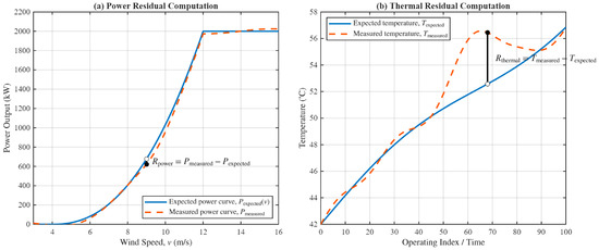
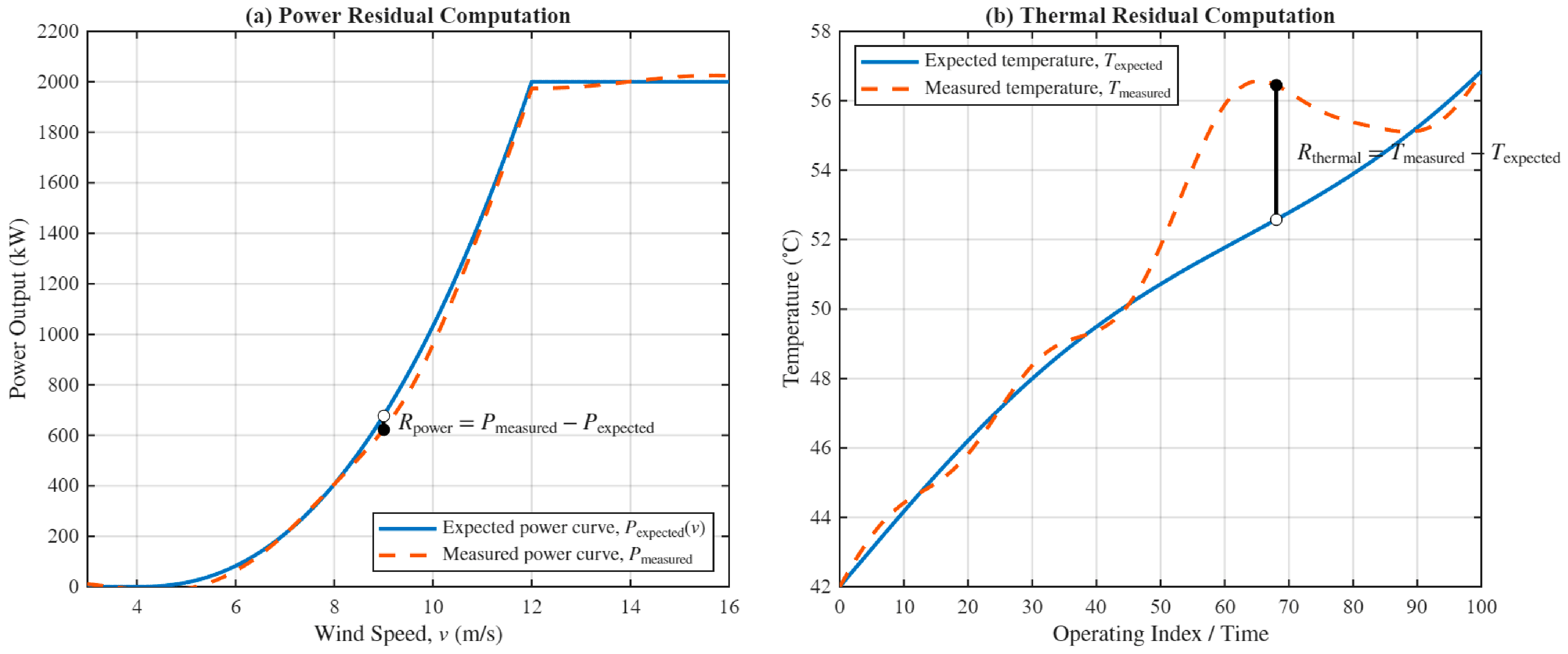
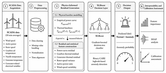
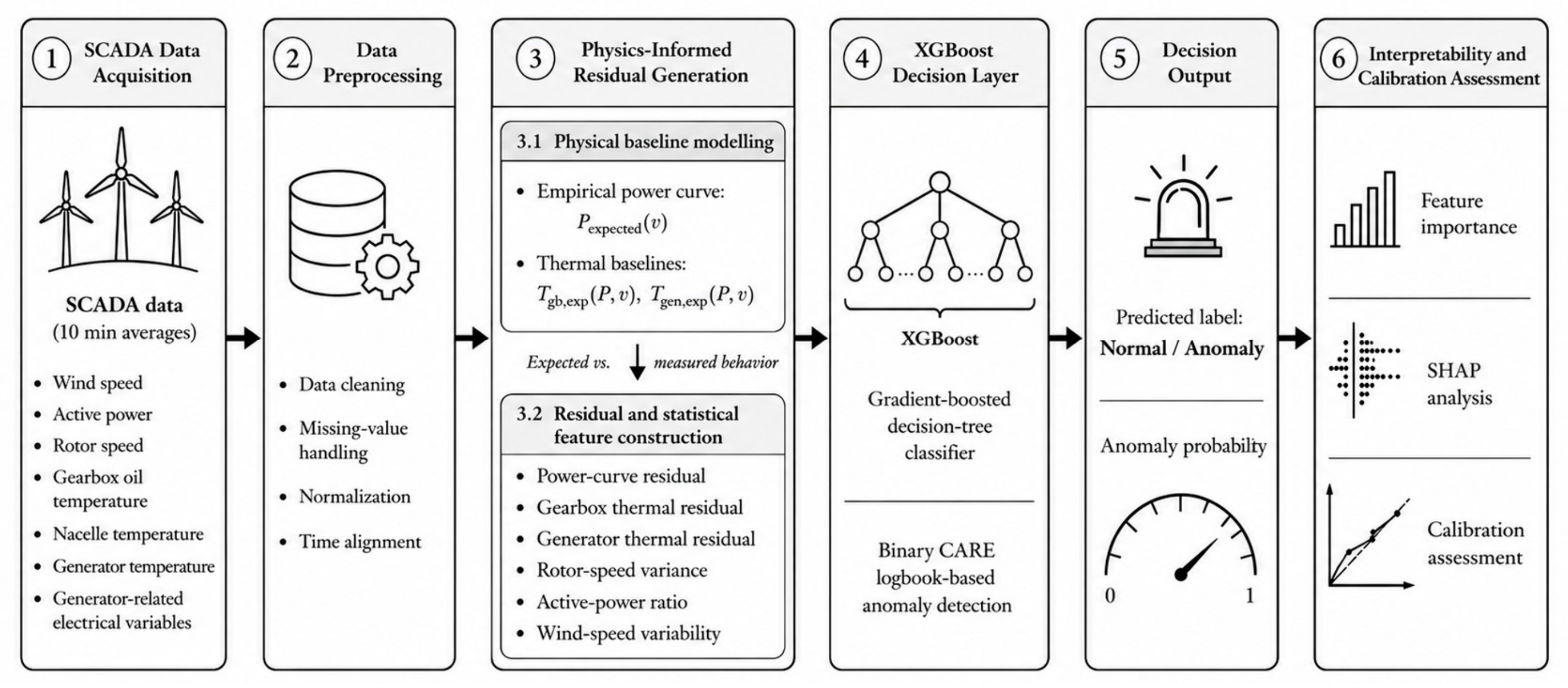
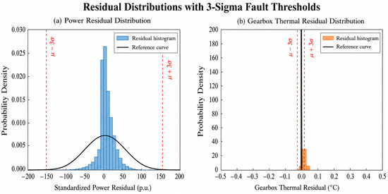
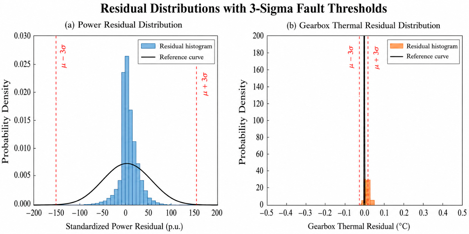
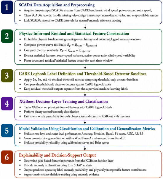
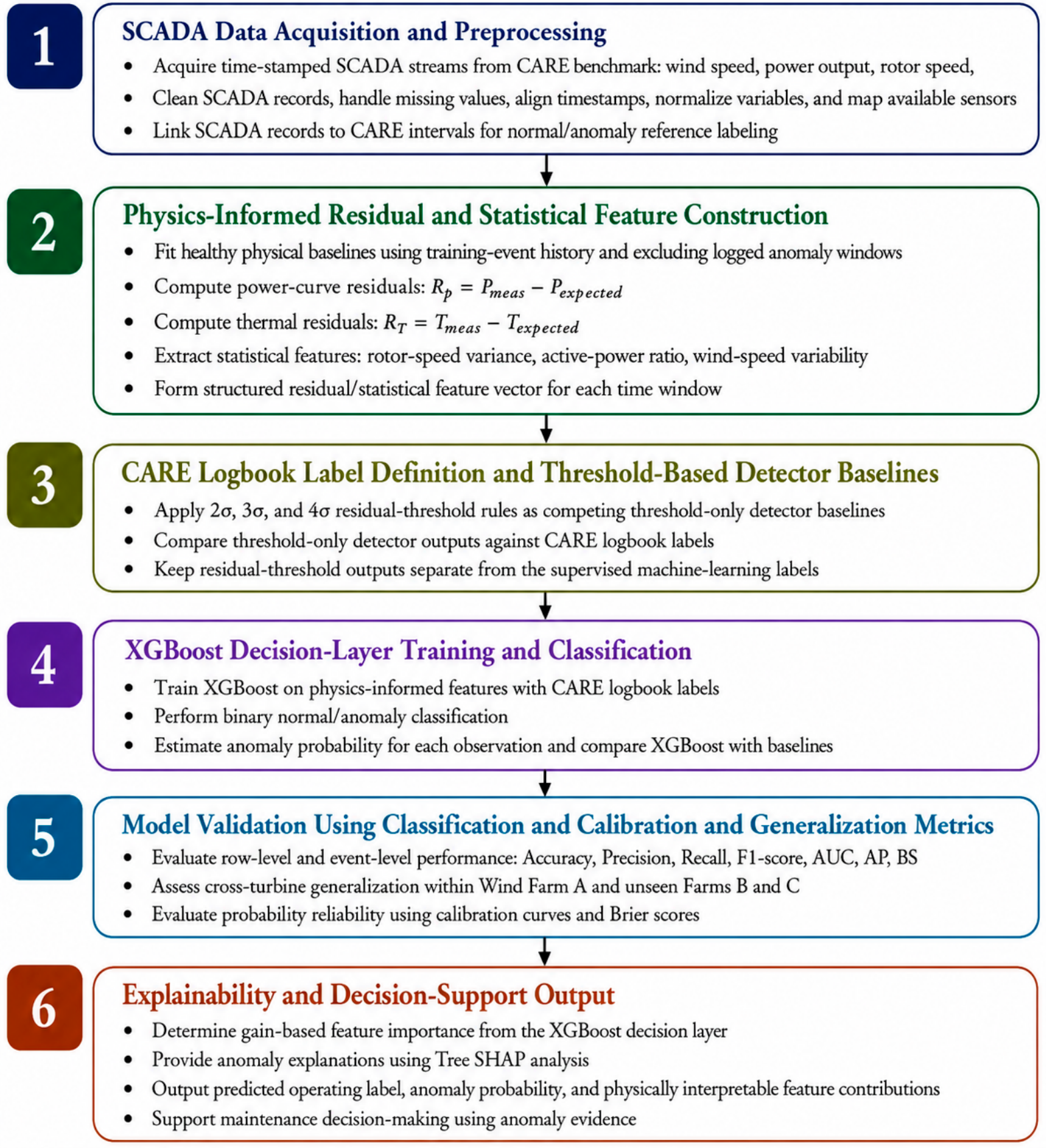
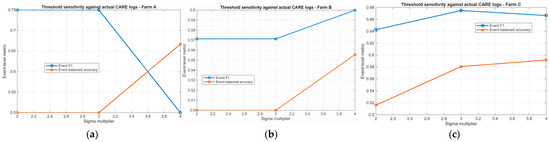
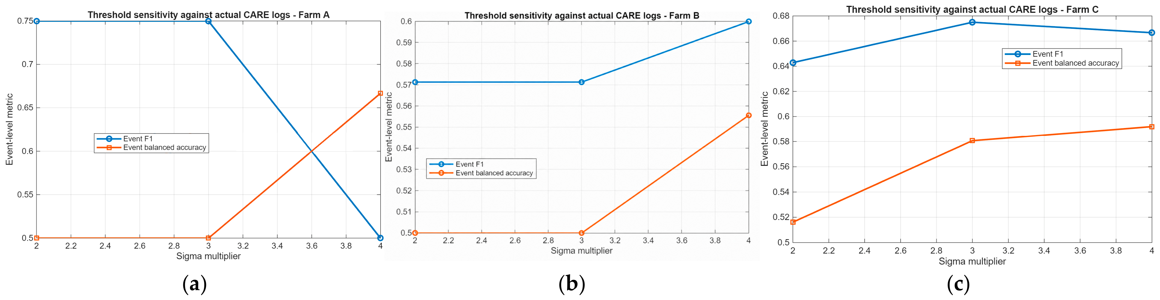
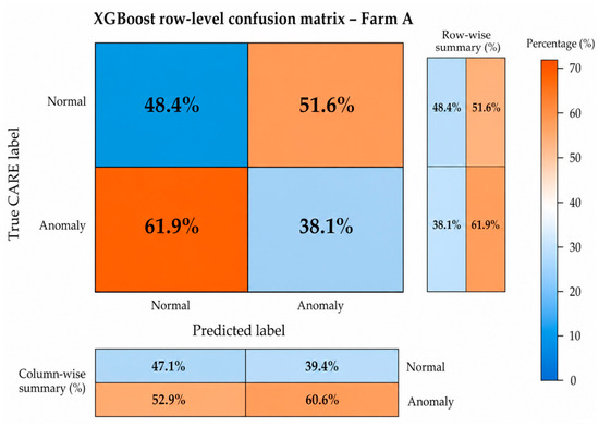
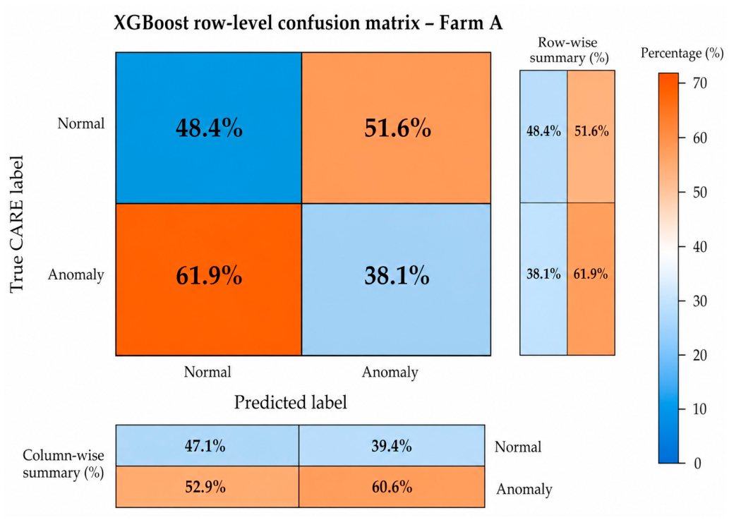
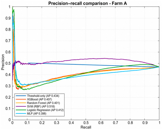
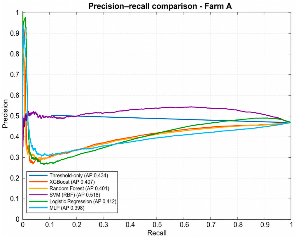
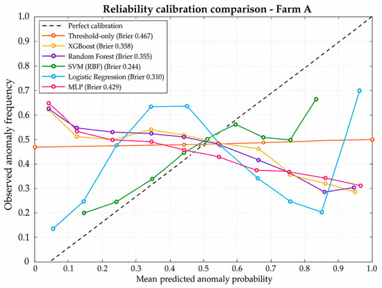
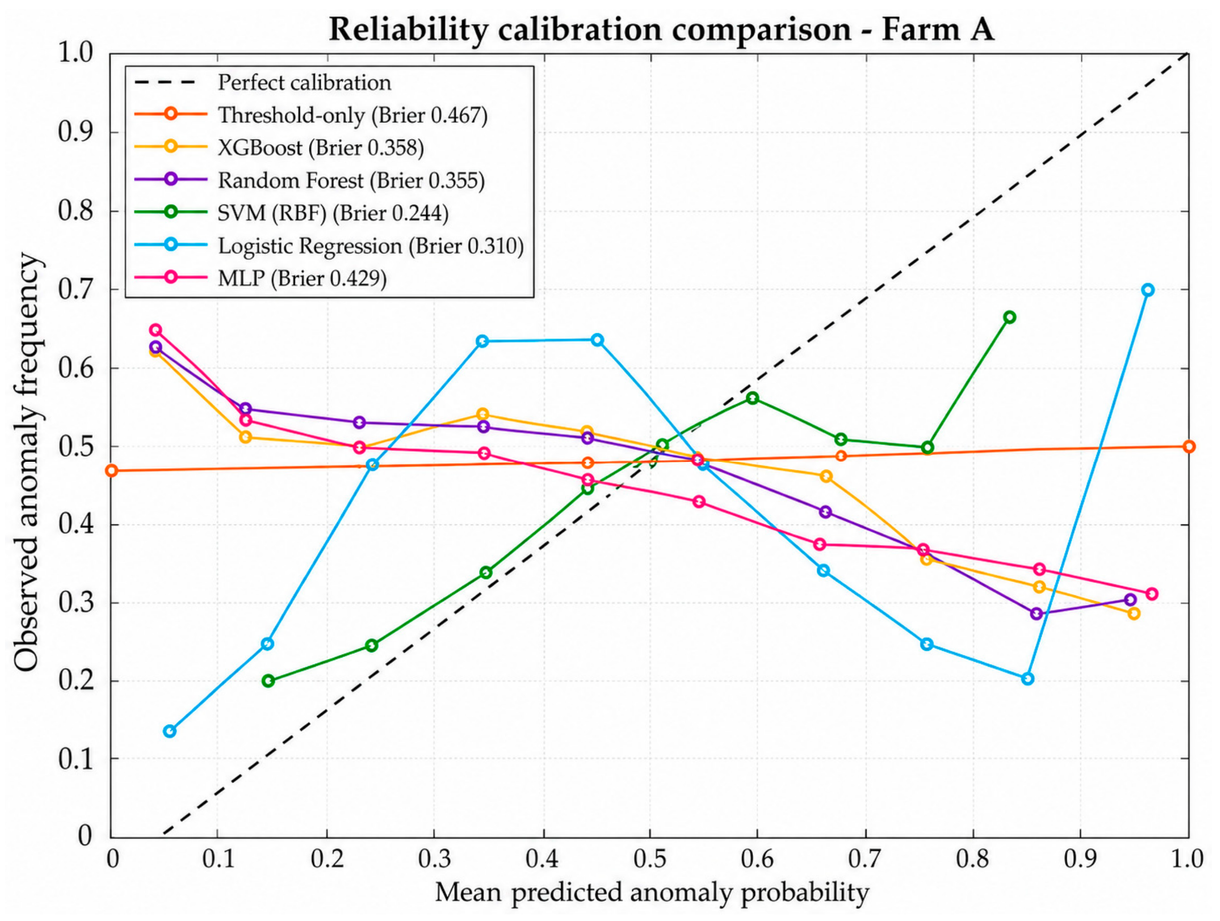
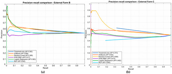
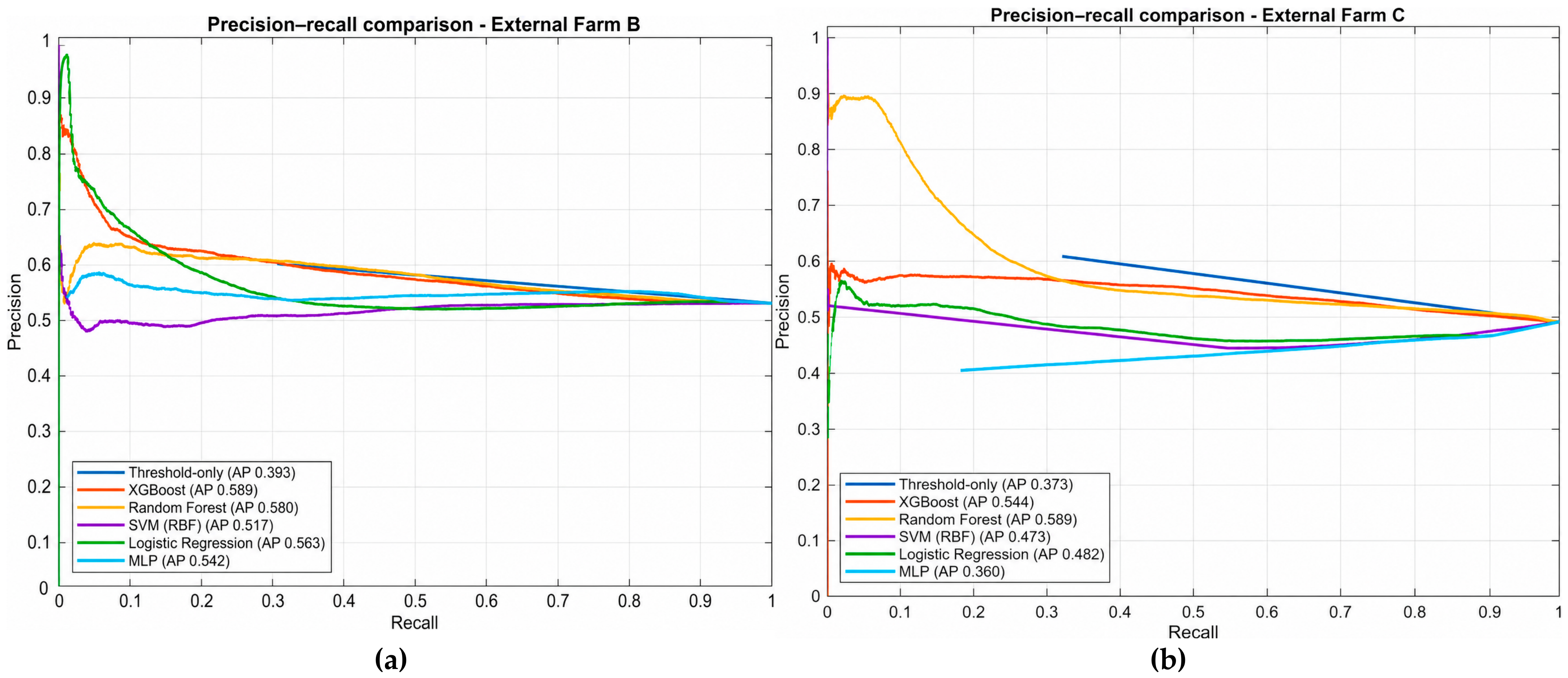
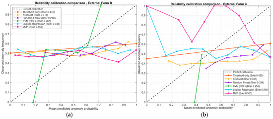
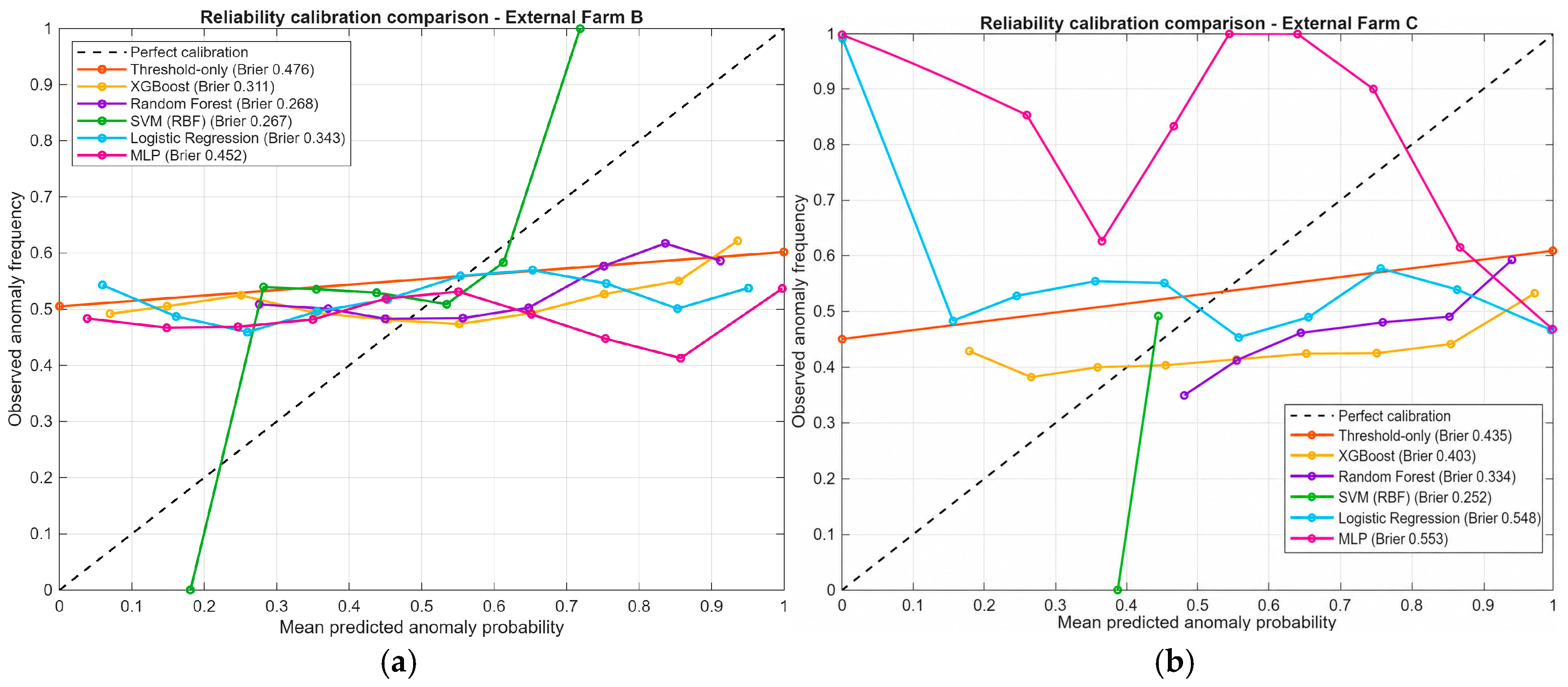
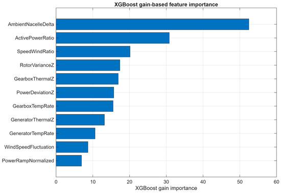
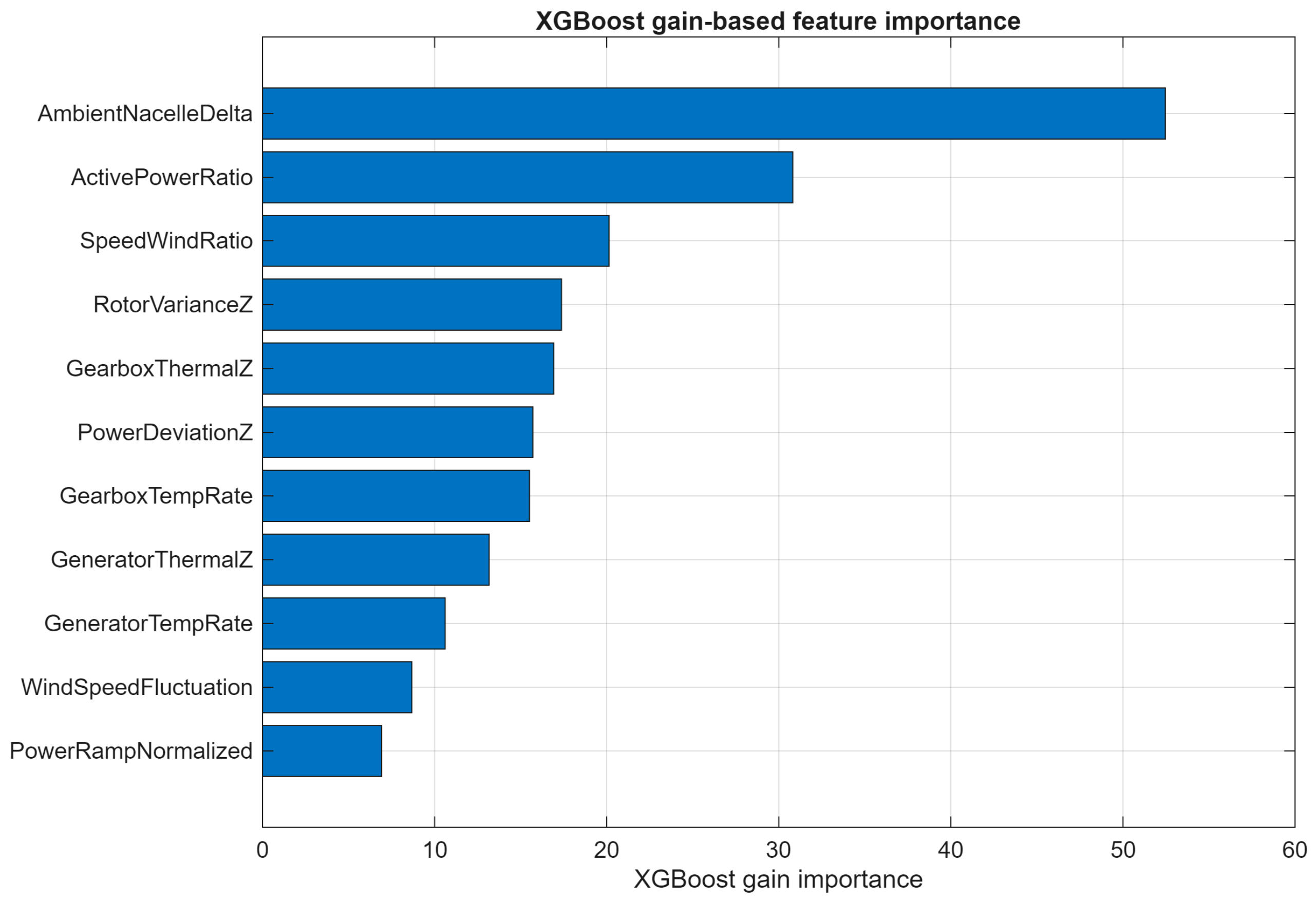
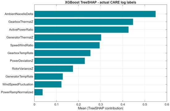
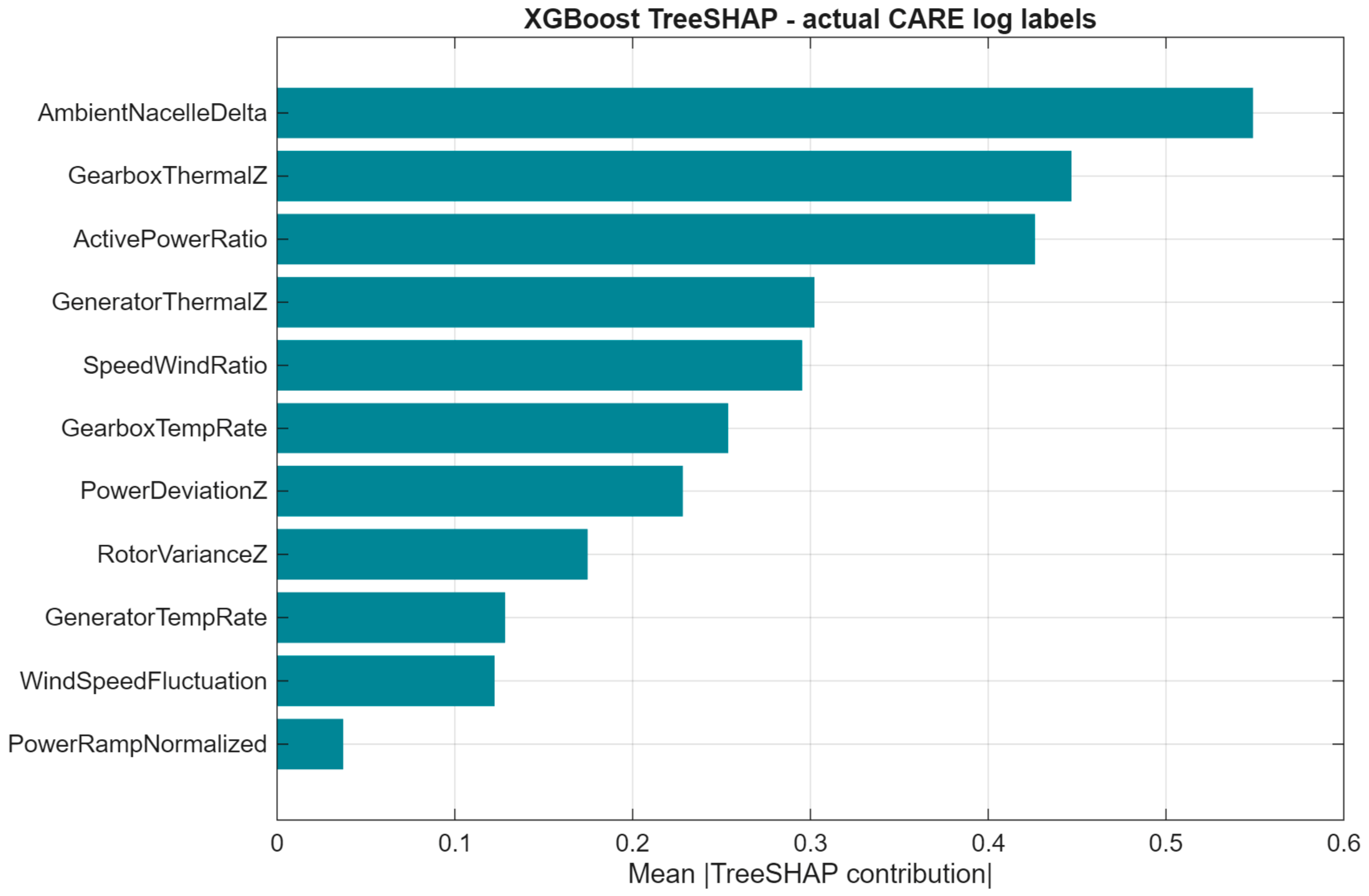
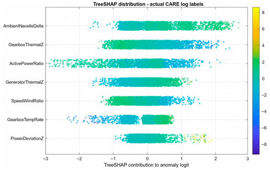
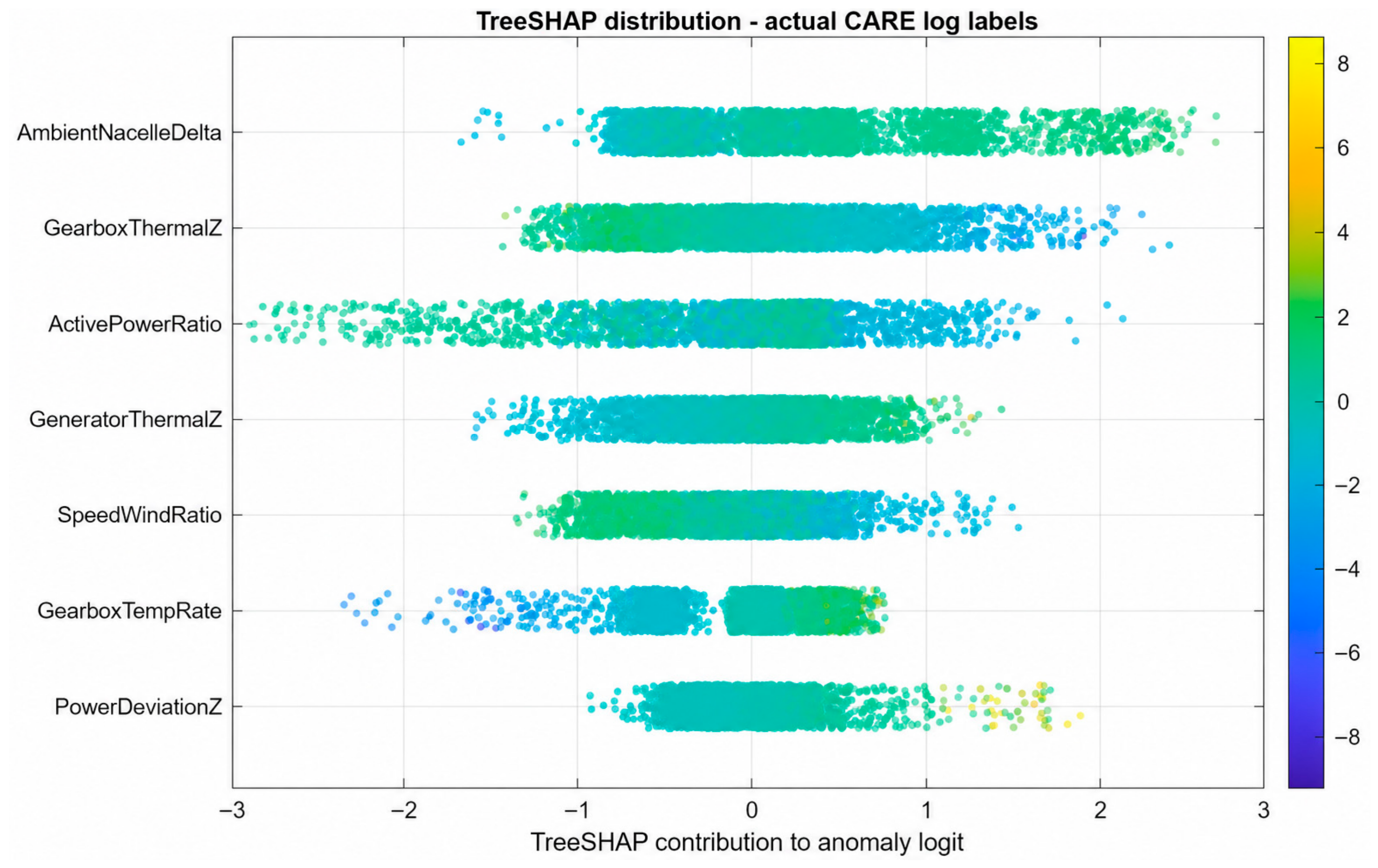

Disclaimer/Publisher’s Note: The statements, opinions and data contained in all publications are solely those of the individual author(s) and contributor(s) and not of MDPI and/or the editor(s). MDPI and/or the editor(s) disclaim responsibility for any injury to people or property resulting from any ideas, methods, instructions or products referred to in the content. |
© 2026 by the authors. Licensee MDPI, Basel, Switzerland. This article is an open access article distributed under the terms and conditions of the Creative Commons Attribution (CC BY) license.