Latent Trajectory Forecasting for Long-Horizon Multivariate Nuclear Power Plant Parameter Prediction

Abstract

Long-horizon multivariate forecasting of nuclear power plant parameters becomes increasingly challenging as the forecast horizon and the number of target variables grow. This study evaluates an long short-term memory (LSTM) autoencoder-based latent trajectory forecasting framework for operator-support-oriented prediction using compact nuclear simulator data. Instead of directly regressing the full future trajectory in the observation space, the proposed framework compresses future trajectories into low-dimensional latent coordinates and predicts those coordinates from short observation histories. Three repeated-seed experiments were conducted to compare direct and latent forecasting across forecast horizons and latent dimensions. Within the direct LSTM baseline considered in this study, direct observation-space forecasting remained competitive at short horizons; whereas, latent trajectory forecasting became increasingly advantageous as the horizon increased. In the 1500-step, 25-channel task, the latent model reduced root mean square error (RMSE) by approximately 16% compared with the direct LSTM baseline while using substantially fewer parameters. Latent-dimension sweeps showed that the smallest bottleneck can have limited representational margin, whereas moderate-to-large dimensions form a broad practical operating range rather than a single universal optimum. These findings suggest that long-horizon nuclear plant parameter prediction can be treated as a conditional trajectory-generation problem in which a short recent plant history is mapped to a compact future-trajectory coordinate, providing a practical, parameter-efficient design direction for AI-assisted plant monitoring and operator support.

1. Introduction

Accurate anticipation of plant behavior during abnormal and emergency situations is central to nuclear power plant (NPP) safety. Operators must identify the evolving state of the plant, determine whether ongoing actions are appropriate, and infer how safety-related variables will change over the next minutes or hours. Physics-based thermal-hydraulic (TH) system codes remain the standard tool for analyzing such behavior, but they are computationally intensive and are therefore difficult to use directly for real-time operator support or for exhaustive simulation campaigns that require thousands of accident scenarios [1,2,3]. This tension has motivated the use of data-driven surrogate models for rapid prediction of future plant parameter trends [1,2,3,4,5,6,7,8,9,10,11].

The first major line of work in this area focuses on direct forecasting in the observation space. In the operator-support setting, Bae et al. compared recursive, direct, and multi-input multi-output (MIMO) strategies with MLP, vanilla RNN, and LSTM models and reported that a MIMO-LSTM combination could predict 25 plant parameters from short observation records and operator actions more accurately than alternative combinations [1]. Other nuclear studies similarly used direct forecasting architectures to predict accident or transient responses from scenario conditions or observed histories [3,4,5,6,7,8,9,10,11]. Across this literature, the dominant modeling choice remains a direct mapping from plant observations or scenario descriptors to future values in the original signal space.

Although these studies establish the feasibility of data-driven trend prediction, most nuclear forecasting settings remain limited in at least one of three ways. First, many studies target only a small set of safety variables or a narrowly defined accident family [3,6,7,8,10,11]. Second, the most common prediction horizons remain on the order of tens to a few hundreds of time steps, even in papers that target longer-term trends [1,2,5,9]. Third, many models are optimized primarily for one forecasting target at a time rather than for scaling behavior as both forecast horizon and the number of target variables increase [1,2,5].

This direct formulation becomes increasingly difficult when both the forecast horizon and the number of target variables grow. In short-horizon or low-dimensional tasks, the model only needs to predict a relatively small output object. However, in long-horizon multivariate forecasting, a short input history must be mapped to a future trajectory with size H × V, where H is the forecast horizon and V is the number of target variables. For example, a 1500-step forecast of 25 variables requires the model to recover 37,500 output values from a short observation window. As H and V increase, the forecasting problem is no longer only a point-wise regression problem; it also becomes a trajectory-scaling problem in which the model must preserve short-term transients, delayed responses, and long-term trend evolution simultaneously [12,13].

Latent or reduced-order representations offer a natural way to address this scaling issue. Instead of directly predicting the full future trajectory, a model can first learn a compact representation of trajectory-level behavior and then predict that representation from the available input information. The closest nuclear study to this perspective is the two-stage model of Bae et al., which used a β-variational autoencoder and Monte Carlo dropout to predict critical safety-parameter trends for more than one thousand time steps with epistemic uncertainty quantification [2]. That study showed the potential of predicting compact latent variables rather than full trajectories directly. However, its input structure was based on scenario-condition variables, and the output was focused on two critical variables rather than a broader multivariate plant-parameter trajectory [2].

Related methodology-domain studies also support the value of reduced or latent representations for high-dimensional temporal prediction. General time-series forecasting has long distinguished recursive, direct, and multiple-output strategies [12,13], while recent long-sequence models such as Informer and the Temporal Fusion Transformer (TFT) have addressed scale and multi-horizon structure, patching, or pretraining in broader forecasting settings [14,15]. Latent and reduced-order forecasting studies have further shown that compact representations can support probabilistic multivariate forecasting, time-series generation, Koopman-based dynamics forecasting, and reduced-order modeling [16,17,18,19,20]. In the nuclear domain, related data-driven and digital-twin studies have compared data-driven and model-driven parameter prediction and investigated online autonomous calibration for NPP digital twins [21,22]. More recent long-sequence backbones such as PatchTST and TimesFM have addressed patching, self-supervised pretraining, or foundation-model forecasting [23,24]. These models are important candidate backbones for future NPP forecasting studies. However, they primarily preserve the general observation-history-to-future-trajectory extrapolation formulation. The present study instead focuses on a formulation-level question: whether a long future plant trajectory can be more efficiently generated or reconstructed by conditioning a learned latent trajectory representation on recent plant observations. This compress-then-predict or latent-space generation perspective has become influential in several high-dimensional domains. In computer vision, latent diffusion models perform the generative process in the latent space of a pretrained autoencoder (AE) rather than directly in pixel space, reducing computational cost for high-resolution synthesis [25]. In Earth-system forecasting, conditional latent diffusion models have similarly been used to encode high-dimensional precipitation or atmospheric fields into compact latent states before generating future states [26,27]. In scientific machine learning, latent DeepONet and latent neural partial differential equation (PDE) solvers learn operators or dynamics in low-dimensional latent spaces and then decode predictions back to physical fields [28,29]. These developments support the broader view that high-dimensional spatiotemporal fields often contain lower-dimensional trajectory structure that can be exploited for prediction, conditional generation, or reduced-order surrogate modeling [16,17,18,19,20,25,26,27,28,29]. Nevertheless, the nuclear forecasting literature has not yet systematically examined when latent trajectory forecasting becomes preferable to direct observation-space forecasting for short-history, long-horizon, multivariate plant-parameter prediction.

Table 1 summarizes representative nuclear-plant parameter forecasting studies and clarifies the positioning of the present study with respect to input information, prediction target, forecast horizon, and methodological focus.

Table 1. Comparison with representative nuclear power plant parameter forecasting studies.

Study	Inputs	Outputs/Horizon	Main Focus
Bae et al. (2021) [1]	Short histories + operator actions	25 plant parameters, 20-step	Direct operator-support forecasting with MIMO-LSTM
Radaideh et al. (2020) [3]	Accident scenario/time-series data	Critical LOCA-related variables	LSTM-based accident trend forecasting
Nguyen et al. (2020) [4]	NPP steam-generator time series	Long-term SG water-level signal	Optimized LSTM for long-term signal prediction
Kim and Kim (2023) [5]	Emergency-condition observations	Safety parameters, 120-step class	Long-term safety-parameter prediction with uncertainty estimation
Wapachi and Diab (2023) [6]	PWR transient time series	PWR response under CEA withdrawal	Transient-response forecasting for accident analysis
Bae et al. (2026) [2]	Scenario-condition inputs	Two critical variables, >1000-step	Latent forecasting with epistemic uncertainty quantification
This study	Short observed multivariate histories	10- and 25-channel tasks, up to 1500-step	Latent trajectory forecasting for long-horizon multivariate operator support

This study addresses that missing comparison. Rather than proposing another forecasting architecture for a fixed benchmark, we ask a structural question: when does latent trajectory forecasting become more advantageous than direct forecasting as the forecasting problem becomes larger? In this paper, forecasting complexity is considered primarily in terms of forecast horizon H and output-variable count V, while the latent dimension D is treated as the main configuration variable controlling the capacity of the latent trajectory representation.

The main contributions of this study are as follows. First, we formulate long-horizon multivariate NPP parameter prediction as a trajectory-scaling problem in which the output object grows with both forecast horizon and output-variable count. Second, we develop and evaluate a two-stage latent trajectory-coordinate forecasting framework that predicts compact future-trajectory coordinates rather than directly regressing the full observation-space trajectory. Third, through repeated-seed horizon-sweep experiments, we show that latent forecasting becomes increasingly advantageous over the direct LSTM baseline as the forecast horizon increases, while a smaller direct LSTM with fewer hidden units does not reproduce the latent model’s long-horizon behavior. Fourth, we empirically characterize latent-dimension effects in a 25-channel, 1500-step task and show that practical configuration is better interpreted as a broad operating range balancing compactness, accuracy, and trajectory robustness. Finally, a same-variable reduced-output control analysis shows that output-variable count alone does not determine the required latent capacity, motivating task-dependent latent-dimension configuration.

2. Methodology

2.1. Problem Formulation

This study considers long-horizon multivariate forecasting of NPP parameters from a short history of observed plant variables. Let X denote the observed input sequence and Y denote the future target trajectory:

$$\mathrm{X}\in {\mathbb{R}}^{\mathrm{L}\times {\mathrm{N}}_{\mathrm{in}}},\mathrm{Y}\in {\mathbb{R}}^{\mathrm{H}\times \mathrm{V}}$$

(1)

Here, L is the input length, N_in is the number of input variables, H is the forecast horizon, and V is the number of target variables. The output object therefore grows with both H and V. The paper compares two forecasting formulations: direct observation-space forecasting, which predicts the full future trajectory directly, and latent trajectory forecasting, which first represents the future trajectory in a lower-dimensional latent space before reconstruction.

In this study, the term trajectory-scaling problem refers to this output-space growth and the associated need to preserve trajectory-level temporal structure as H and V increase. It is not intended to denote a different physical forecasting problem from conventional multi-step prediction; rather, it emphasizes that the prediction target becomes a high-dimensional future trajectory whose dimension and structural complexity scale with both forecast horizon and output-variable count.

2.2. Direct Observation-Space Forecasting

The direct forecasting baseline learns a direct mapping from the short observation history to the full future trajectory:

$$\widehat{\mathrm{Y}}={\mathrm{f}}_{\mathrm{d}\mathrm{i}\mathrm{r}}\left(\mathrm{X}\right)$$

(2)

Because the network output is the complete future trajectory, the direct model must learn all point-wise values and trajectory-level temporal structures in the original observation space. This formulation is simple and effective for short horizons, but the output-space burden increases rapidly as H and V grow.

The direct LSTM baseline is therefore used as an observation-space regression baseline aligned with prior operator-support forecasting work [1]. It is not intended to represent all modern long-sequence forecasting architectures. Instead, it provides a controlled reference for evaluating whether moving the prediction target from the full observation space to a compact latent trajectory coordinate changes the scaling behavior of the forecasting task.

2.3. Latent Trajectory Forecasting Framework

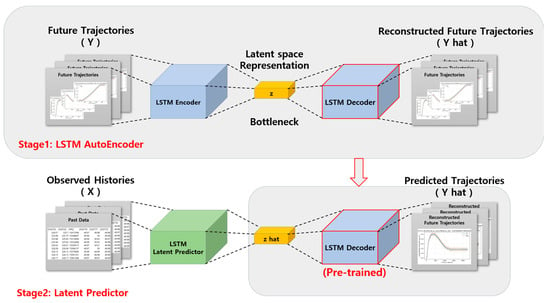
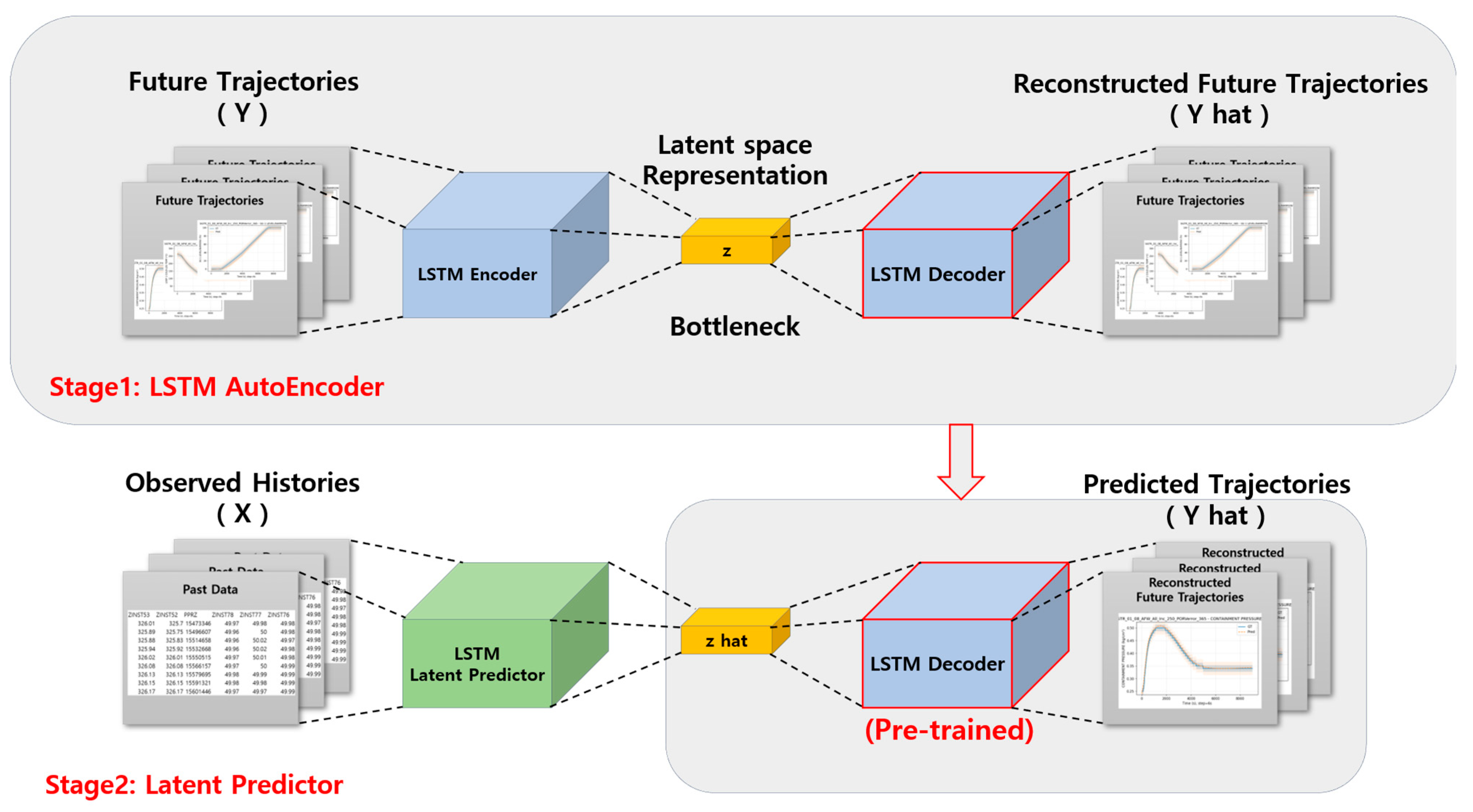
The proposed latent trajectory forecasting framework is shown in Figure 1. It separates trajectory representation learning from short-history forecasting. In Stage 1, an LSTM autoencoder learns to compress each future trajectory into a D-dimensional latent vector and reconstruct the original trajectory from that vector. In Stage 2, a separate LSTM predictor maps the observed history to the latent coordinate, and the pre-trained decoder reconstructs the full future trajectory.

Figure 1. Two-stage LSTM autoencoder-based latent trajectory forecasting framework.

In the autoencoder stage, the future trajectory is encoded into a D-dimensional latent vector:

$$\mathrm{z}=\mathrm{E}\left(\mathrm{Y}\right), \mathrm{z}\in {\mathbb{R}}^{\mathrm{D}}$$

(3)

The decoder then reconstructs the trajectory from the latent vector:

$${\widehat{\mathrm{Y}}}_{\mathrm{A}\mathrm{E}}=\mathrm{D}\mathrm{e}\mathrm{c}(\mathrm{z})$$

(4)

After the autoencoder is trained, the decoder is fixed and a history-to-latent predictor is trained:

$$\widehat{\mathrm{z}}=\mathrm{g}\left(\mathrm{X}\right)$$

(5)

The final trajectory prediction is obtained by decoding the predicted latent vector using the pre-trained decoder:

$$\widehat{\mathrm{Y}}=\mathrm{D}\mathrm{e}\mathrm{c}(\widehat{\mathrm{z}})$$

(6)

In this formulation, the predictor does not directly regress the full H × V future trajectory. Instead, it predicts a compact D-dimensional coordinate that summarizes trajectory-level behavior. The decoder then maps this coordinate back to the multivariate future trajectory. This structure reduces the effective regression burden from the full output space to the latent coordinate space while retaining a decoder-based trajectory prior.

Here, Enc(.) and Dec(.) denote the autoencoder encoder and decoder, z is the latent coordinate of the future trajectory, z_hat is the predicted latent coordinate obtained from the observed history X, and Y_hat is the reconstructed future trajectory. The functions f_direct(.) and g_latent(.) denote the direct observation-space predictor and the history-to-latent predictor, respectively. These definitions are added to make the mapping roles in Equations (2)–(6) explicit.

The latent dimension D controls the capacity of the trajectory representation. If D is too small, the latent space may be unable to distinguish important transient patterns, delayed responses, or long-term recovery trends, resulting in under-capacity behavior. If D is sufficiently large, additional dimensions may provide only marginal improvement. Therefore, this study interprets D in terms of a practical operating range rather than a single universally optimal bottleneck size.

2.4. Model Architecture and Inference Procedure

The latent forecasting framework was implemented using an LSTM autoencoder and an LSTM-based history-to-latent predictor. The autoencoder used an LSTM encoder and decoder to learn trajectory-level representations from future target sequences. The predictor used the short observed plant history as input and produced the latent coordinate required by the decoder.

Training followed the two-stage procedure illustrated in Figure 1. First, the autoencoder was trained to reconstruct future trajectories. Second, the decoder was frozen, and the predictor was trained so that the decoded predicted latent vector matched the future trajectory. This separation makes the forecasting model learn compact trajectory coordinates while preserving the decoder as a learned trajectory reconstruction map. The stepwise procedure is summarized in Table 2.

Table 2. Two-stage latent trajectory forecasting procedure.

Phase	Step	Operation	Output
Training: trajectory representation	1	Construct future trajectory samples Y from simulator records.	Trajectory samples
Training: trajectory representation	2	Train LSTM encoder–decoder so that Dec(Enc(Y)) reconstructs Y.	Encoder, decoder, latent coordinates z
Training: history-to-latent prediction	3	Freeze the pre-trained decoder and train an LSTM predictor that maps observed history X to z_hat.	History-to-latent predictor
Inference	4	Given a short recent history X, predict z_hat and decode Dec(z_hat).	Long-horizon multivariate forecast Y_hat

3. Experimental Setup and Results

3.1. Dataset and Forecasting Tasks

The experiments were conducted on compact nuclear simulator (CNS) data following the operator-support forecasting context of Bae et al. (2021) [1] but extended to longer three-hour simulator records for long-horizon prediction. The CNS represents a simplified Westinghouse 1000 MWe three-loop pressurized water reactor and was used in the reference study to generate emergency operation data for loss-of-coolant accident (LOCA), steam-generator tube rupture (SGTR), and simple reactor-trip scenarios. The original scenario generation analyzed CNS emergency operating procedures and varied action timing, action degree, and prerequisite completion to represent diverse operator-action outcomes. The present study uses the same input- and target-variable definitions as that operator-support dataset, while extending the future prediction horizon from the 10 min setting in [1] to up to 2.5 h at 6 s resolution. The dataset, preprocessing, and scenario configuration are summarized in Table 3.

Table 3. Dataset, preprocessing, and scenario configuration used in this study.

Item	Configuration/Description
Simulator basis	Compact nuclear simulator (CNS), following the operator-support dataset of Bae et al. [1].
Accident families	LOCA, SGTR, and simple reactor trip scenario families, including operator-action variations.
Reference scenario counts	Bae et al. generated 1153 emergency-operation scenarios: 865 LOCA, 200 SGTR, and 98 simple-trip cases [1].
Scenario-file split in this work	Among 1153 scenario files, 1118 files were used as the training pool and 35 files were held out for test evaluation at the scenario-file level.
Raw resolution and record length	1 s raw simulator records extended to three-hour records.
Input variables	109 plant variables: 25 target parameters plus 84 valve states, component states, instrument values, and important plant signals.
Output variables	Main 25-channel critical safety function (CSF) monitoring target set and nested reduced 10-channel subset.
Normalization	Min–max normalization computed from training files only; same statistics applied to validation/test data.
Window generation	Training windows generated by sliding window with 1 s shift and capped at 100 windows per training file; held-out test evaluation uses one action-related sample per test scenario.
Operator-action set	Emergency-procedure-based actions include auxiliary feedwater flow control, reactor coolant pump stop, power-operated relief valve (PORV) shut-off valve opening, PORV opening, safety-injection signal reset, safety-injection pump stop, main steam line isolation, secondary-side relief valve manual opening, contaminated steam line isolation, and no-action cases; action timing, degree, and prerequisite completion were varied following [1].
Validation split	Window-level validation split of 0.1 from the training-window pool for early stopping/model selection; all reported test results were computed on held-out scenario files.

For the main experiments, forecasting trajectories were sampled at 6 s intervals. Therefore, H = 1500 corresponds to approximately 9000 s, or 2.5 h, of future prediction. Each forecasting sample used five observed input steps constructed from 109 plant variables. These input variables included the 25 prediction target parameters as well as 84 additional variables consisting of valve states, component states, instrument values, and important plant signals.

The short observation history was intentionally retained for operator-support-oriented forecasting. In this setting, the most relevant conditional information is expected to be concentrated in the recent post-action or rapidly changing segment of the plant trajectory; waiting for a long observation history would reduce the practical value of early operator support. The five-step history at 6 s sampling therefore represents a short recent window on the order of 30 s, while the inclusion of 109 plant and action-related signals provides the conditioning information needed to forecast the subsequent long-horizon trajectory.

Three forecasting tasks were used to examine horizon scaling, latent-dimension sensitivity, and reduced-output behavior. The task definitions are summarized in Table 4.

Table 4. Main forecasting tasks used in the manuscript.

Task	Input Shape	Output Channels	Forecast Horizon	Purpose
Horizon sweep	(5, 109)	25	20/100/500/1500	Direct-versus-latent scaling behavior
25-channel z sweep	(5, 109)	25	1500	Hardest-task latent-dimension analysis
Reduced-output z sweep	(5, 109)	10	1500	Reduced-output practical range analysis

3.2. Target Variables and Output Configurations

The 25-channel output task followed the prediction target set of Bae et al. (2021) [1]. The target variables consist of critical-safety-function monitoring parameters, including reactor power, neutron range indicators, core and loop temperatures, pressurizer pressure and level, steam-generator levels and pressures, feedwater flows, and containment variables.

The reduced 10-channel task was selected from the 25-channel set to retain plant-wide subsystem coverage while removing repeated loop-wise measurements. The reduced set consisted of power range percent power, core outlet temperature, pressurizer pressure, steam generator (SG) 1 narrow-range level, auxiliary feedwater flow 1, SG 1 pressure, Loop 1 cold-leg temperature, containment pressure, containment sump water level, and pressurizer level. The complete target-variable lists are provided in Appendix A.

3.3. Training Settings and Evaluation Metrics

The direct baseline used an LSTM predictor that mapped the short observation history directly to the full future trajectory. In the horizon-sweep experiments, direct models with hidden sizes U = 512 and U = 256 were used as reference baselines. The U = 512 model served as the main direct baseline, while the smaller direct LSTM with fewer hidden units (U = 256) was included at H = 1500 as a lower-parameter control baseline.

The latent models used the same LSTM autoencoder-based architecture family across experiments. The autoencoder consisted of a 256-unit LSTM encoder and a 256-unit LSTM decoder, and the history-to-latent predictor also used 256 LSTM units. During predictor training, the decoder was fixed. The horizon sweep used D = 16 as a compact reference latent dimension, while the latent-dimension sweeps varied D to evaluate the effect of bottleneck capacity. The training configurations used in the main experiments are summarized in Table 5.

Table 5. Training configurations used in the main experiments.

Experiment	Model	Main Configuration	Training Settings
Horizon sweep	Direct LSTM	25 output channels; H = 20, 100, 500, and 1500; U = 512, with U = 256 also evaluated at H = 1500	Batch 64; max 1000 epochs; patience 30; learning rate 0.001
Horizon sweep	Latent forecasting	LSTM AE + latent predictor; D = 16; encoder, decoder, and predictor hidden units = 256; decoder fixed during predictor training	Batch 64; max 1000 epochs; patience 30; learning rate 0.001
Latent-dimension sweeps	AE + predictor	H = 1500; output channels = 25 or 10; D varied; predictor input shape = (5, 109)	AE: batch 64, max 300 epochs, patience 20; predictor: batch 128, max 2000 epochs, patience 30; learning rate 0.001

All experiments used min–max normalization computed from the training files only, and forecasting windows were generated using the sliding-window procedure summarized in Table 3. The same training-set normalization statistics were applied to validation and held-out test samples to avoid test-set information leakage. Because the present dataset is simulator-derived CNS data rather than direct plant measurement data, stochastic sensor noise was not explicitly injected or filtered in this study. No smoothing filter was applied before training so that rapid transient responses following operator actions were preserved. The main experimental conditions were repeated using random seeds 42, 43, and 44, and the reported quantitative tables provide mean ± standard deviation across the three runs. Robustness to measured plant noise remains an important follow-up topic for deployment-oriented validation.

The horizon-sweep and latent-dimension-sweep experiments used two training schedules because they were designed to answer different questions. The horizon sweep used a common long training schedule for direct and latent models to support the direct-versus-latent scaling comparison across forecast horizons. In contrast, the z-sweep experiments fixed the hardest 1500-step setting and evaluated multiple latent dimensions across repeated seeds; therefore, a shorter autoencoder early-stopping patience and a longer predictor schedule were used to make the repeated latent-capacity analysis computationally feasible while keeping the architecture family, optimizer, loss, and normalization procedure consistent across the 25-channel and reduced-output z sweeps.

RMSE was used as the primary evaluation metric because it is sensitive to large deviations in long-horizon forecasts. MAE was used as a secondary point-wise error metric, and dynamic time warping (DTW) was used as a shape-based trajectory similarity metric. For a test set with predicted values y_hat and ground-truth values y, MAE is the mean absolute difference, and RMSE is the square root of the mean squared difference over the evaluated samples, time steps, and target variables. MSE was not tabulated separately because RMSE is the square-root form of the same squared-error quantity and is easier to interpret on the normalized target scale. All normalized metrics in the main results are reported as mean ± standard deviation over the three repeated seeds.

A tolerance-based success rate was used only as a complementary trajectory-acceptability indicator. A trajectory-variable forecast was classified as successful when no more than 10% of its predicted points fell outside a ±10% range-based tolerance band. This threshold is not used as the primary accuracy metric; rather, it provides an interpretable robustness indicator for whether the overall predicted trajectory remains within an acceptable band for most of the forecast horizon. For repeated-seed experiments, the tolerance-based success rate is reported as mean ± standard deviation across the three seeds.

3.4. Results

3.4.1. Horizon-Scaling Comparison

Table 6 summarizes the three-seed horizon-sweep results for the 25-channel output task. At H = 20, direct forecasting remained competitive, achieving slightly lower MAE and DTW than the latent model, while the latent model showed a lower RMSE. From H = 100 onward, latent forecasting outperformed the direct baseline across the main normalized error metrics, and the improvement became more pronounced at H = 500 and H = 1500.

Table 6. Horizon-sweep performance for the 25-channel task.

H	Model	MAE	RMSE	DTW	Tolerance-Based Success Rate (%)
20	Direct (U = 512)	0.00443 (0.00013)	0.01407 (0.00246)	0.000817 (0.000015)	99.70 (0.07)
20	Latent (D = 16)	0.00455 (0.00026)	0.01118 (0.00379)	0.000890 (0.000046)	99.81 (0.07)
100	Direct (U = 512)	0.00843 (0.00038)	0.02151 (0.00192)	0.001264 (0.000067)	97.79 (0.35)
100	Latent (D = 16)	0.00684 (0.00013)	0.01693 (0.00088)	0.000983 (0.000027)	98.74 (0.23)
500	Direct (U = 512)	0.01185 (0.00071)	0.02510 (0.00163)	0.001298 (0.000047)	96.38 (0.24)
500	Latent (D = 16)	0.00856 (0.00060)	0.02147 (0.00065)	0.000789 (0.000012)	98.63 (0.20)
1500	Direct (U = 512)	0.01537 (0.00023)	0.03309 (0.00044)	0.001720 (0.000000)	95.58 (0.59)
1500	Direct (U = 256)	0.01588 (0.00043)	0.03248 (0.00065)	0.001814 (0.000093)	95.77 (0.71)
1500	Latent (D = 16)	0.01117 (0.00035)	0.02765 (0.00090)	0.001088 (0.000019)	98.40 (0.20)

Note: Bold values indicate the best mean performance within each forecast horizon for each metric. Lower values are better for MAE, RMSE, and DTW, whereas higher values are better for the tolerance-based success rate.

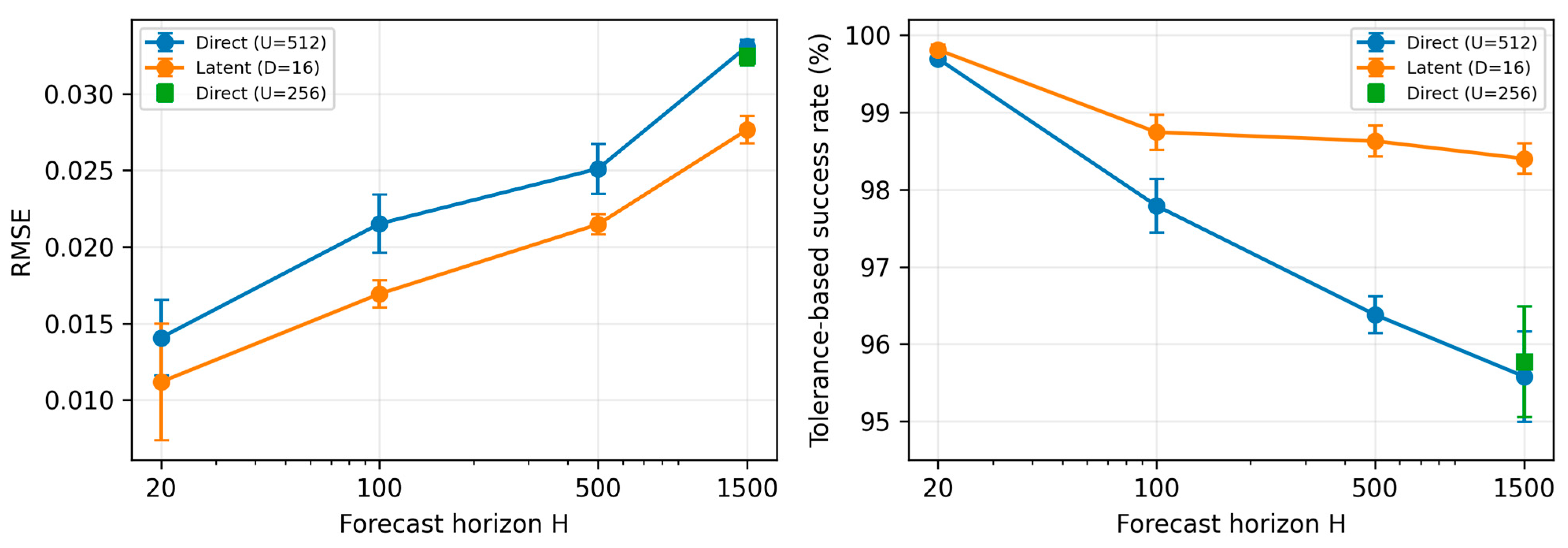
The improvement became most evident in the longest-horizon setting. At H = 1500, the direct LSTM baseline with U = 512 achieved an RMSE of 0.03309 ± 0.00044; whereas, the latent forecasting model with D = 16 achieved an RMSE of 0.02765 ± 0.00090. The smaller direct LSTM with fewer hidden units (U = 256) achieved an RMSE of 0.03248 ± 0.00065. This smaller direct model was included as a control to examine whether the latent-model advantage could be explained merely by reducing the number of trainable parameters. Although the smaller direct model reduced parameter count, it did not approach the latent model across the main long-horizon metrics, supporting the interpretation that the latent formulation provides a structural advantage by predicting compact trajectory coordinates rather than the full observation-space future trajectory directly. The corresponding parameter-count comparison is summarized in Table 7.

Table 7. Parameter-count comparison at H = 1500.

Model	Total Parameters	Relative
Direct (U = 512)	20.51 M	1.0×
Direct (U = 256)	10.01 M	0.49×
Latent AE only	0.58 M	0.028×
Latent AE + predictor	0.92 M	0.045×

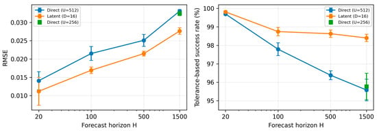
Figure 2 summarizes the same pattern visually using repeated-seed mean values with standard-deviation error bars. The mean RMSE gap between direct and latent forecasting widened as the forecast horizon increased. In addition, the parameter-count comparison at H = 1500 showed that the latent model achieved better long-horizon accuracy with substantially fewer parameters than either direct baseline. These repeated-seed results indicate that the latent advantage is not attributable to a single favorable training run and that latent trajectory forecasting becomes increasingly attractive as the forecast horizon grows.

Figure 2. Quantitative summary of the horizon-sweep experiment.

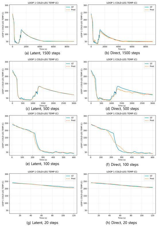
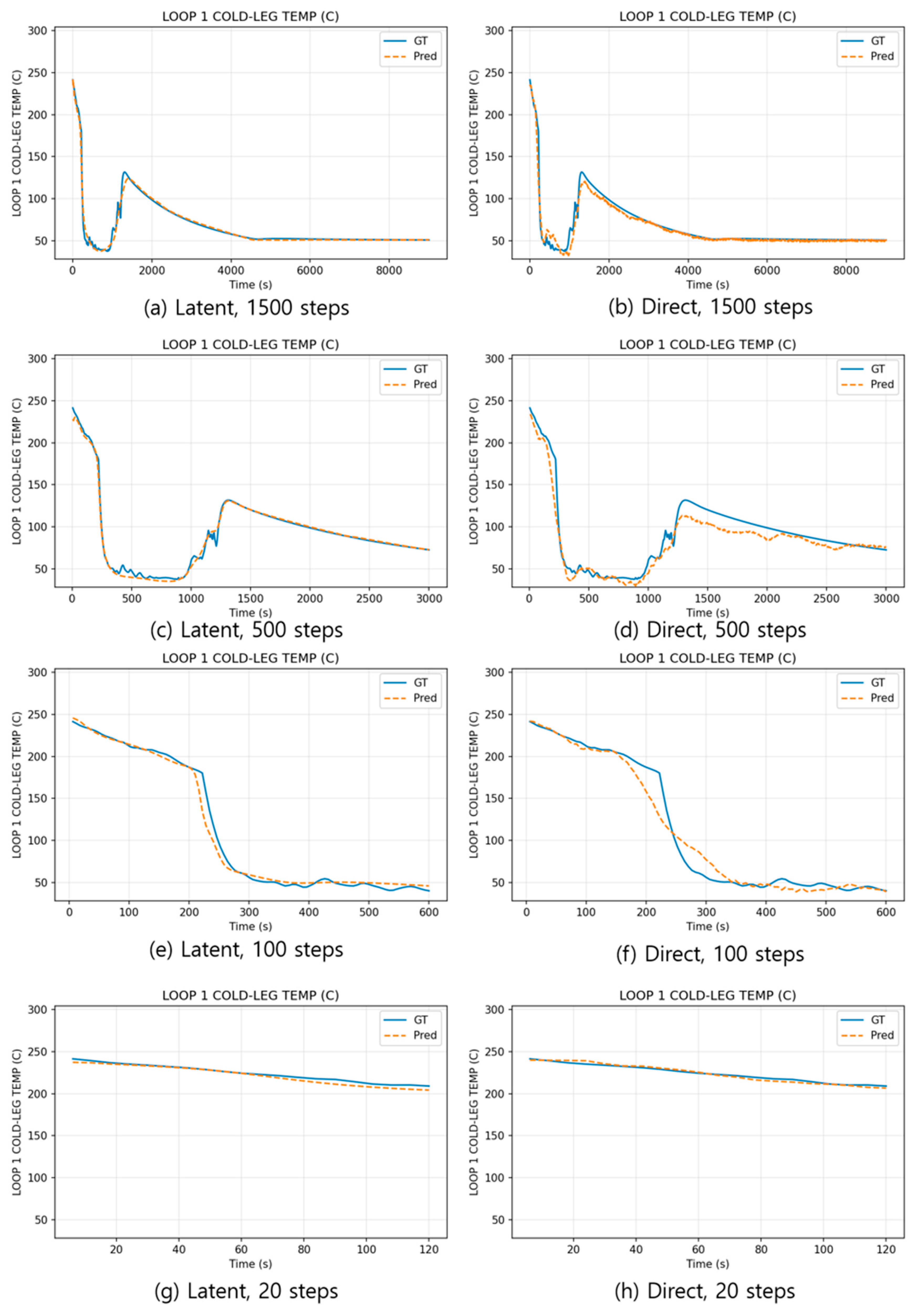
Figure 3 provides a representative trajectory-level comparison for Loop 1 cold-leg temperature in the LOCA_01_45_E1_540_AFW_Inc_600_PORVerror_650 scenario. In this scenario, a 45 cm² LOCA occurred at 10 s, the E0 emergency operating procedure was followed until 540 s, the procedure then transitioned to E1, and the PORV was opened at 650 s. Figure 3a,b compares the latent and direct forecasts at H = 1500, Figure 3c,d) at H = 500, Figure 3e,f at H = 100, and Figure 3g,h at H = 20. The short-horizon forecasts are visually similar; whereas, the longer-horizon forecasts show that the latent model preserves the overall cooling, recovery, and stabilization trend more consistently than the direct baseline.

Figure 3. Representative horizon-sweep trajectory comparison.

3.4.2. Latent-Dimension Analysis in the 25-Channel Task

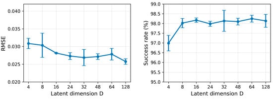
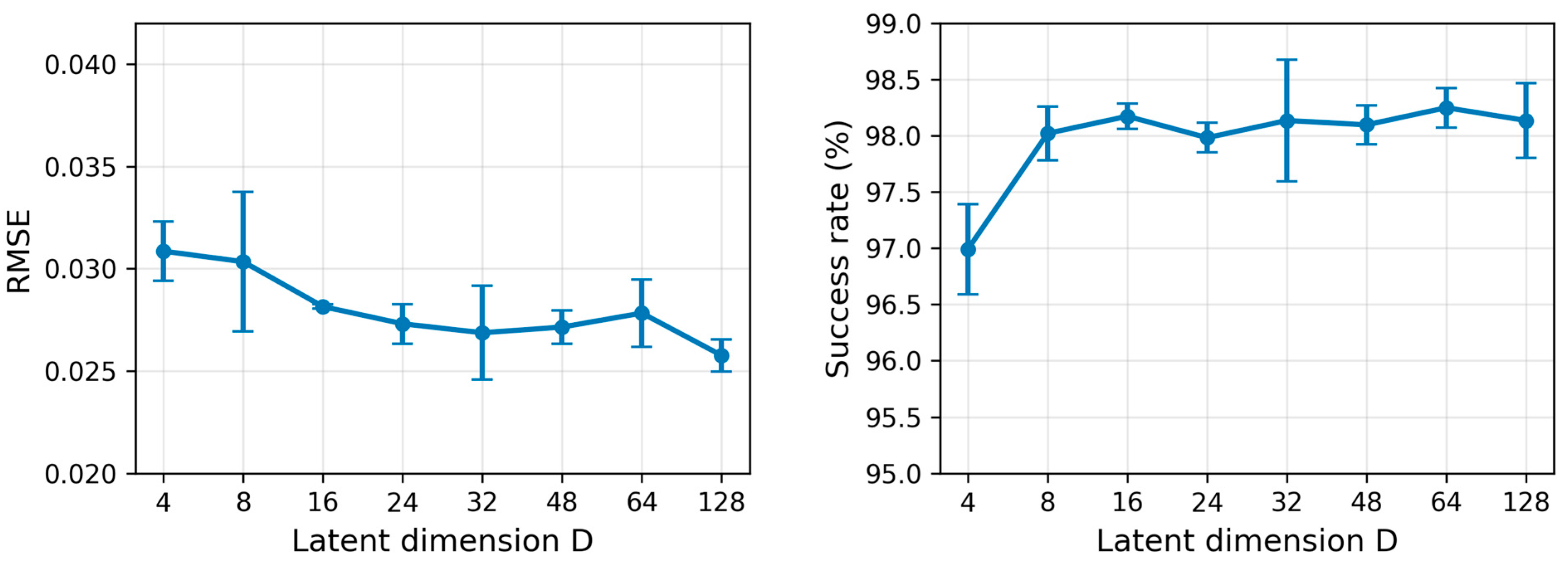
The 25-channel latent-dimension sweep was conducted at H = 1500, which represents the hardest forecasting setting in this study. Table 8 reports mean and standard deviation across seeds 42, 43, and 44. The smallest tested bottleneck, D = 4, showed weaker average performance than several larger latent dimensions; whereas, D = 16 and above formed a broad practical range. The sweep therefore supports a capacity-margin interpretation rather than a single sharply optimal latent dimension.

Table 8. Latent-dimension sweep in the 25-channel task.

D	MAE	RMSE	DTW	Tolerance-Based Success Rate (%)
4	0.01200 (0.00024)	0.03085 (0.00145)	0.001161 (0.000044)	96.99 (0.40)
8	0.01159 (0.00045)	0.03034 (0.00341)	0.001143 (0.000030)	98.02 (0.24)
16	0.01085 (0.00047)	0.02815 (0.00011)	0.001058 (0.000075)	98.17 (0.11)
24	0.01071 (0.00020)	0.02730 (0.00097)	0.001073 (0.000015)	97.98 (0.13)
32	0.01137 (0.00109)	0.02686 (0.00230)	0.001138 (0.000141)	98.13 (0.54)
48	0.01078 (0.00030)	0.02714 (0.00082)	0.001065 (0.000030)	98.10 (0.17)
64	0.01083 (0.00059)	0.02783 (0.00164)	0.001089 (0.000055)	98.25 (0.17)
128	0.01054 (0.00037)	0.02576 (0.00079)	0.001035 (0.000052)	98.13 (0.33)

The results do not indicate a single universal optimum. The lowest mean RMSE was observed at D = 128, while D = 24, 32, 48, and 64 remained competitive with lower dimensionality and similar tolerance-based success rates. Therefore, the practical operating region is better interpreted as a trade-off between compactness, point-wise error, and trajectory-level tolerance robustness rather than as a purely RMSE-optimal single value.

Figure 4 visualizes the RMSE trend and the tolerance-based success rate using mean values with standard-deviation error bars. The weaker average behavior at D = 4 suggests that the smallest tested bottleneck can have limited representational margin in the 25-channel, 1500-step task. However, the repeated-seed results also show that several intermediate-to-large latent dimensions behave similarly, indicating that the practical question is to identify a reliable operating range rather than a single best latent dimension.

Figure 4. Quantitative summary of the 25-channel latent-dimension sweep.

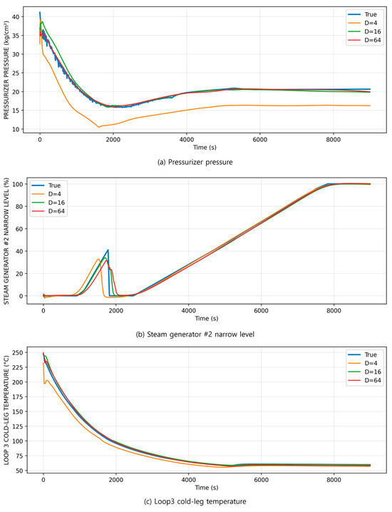
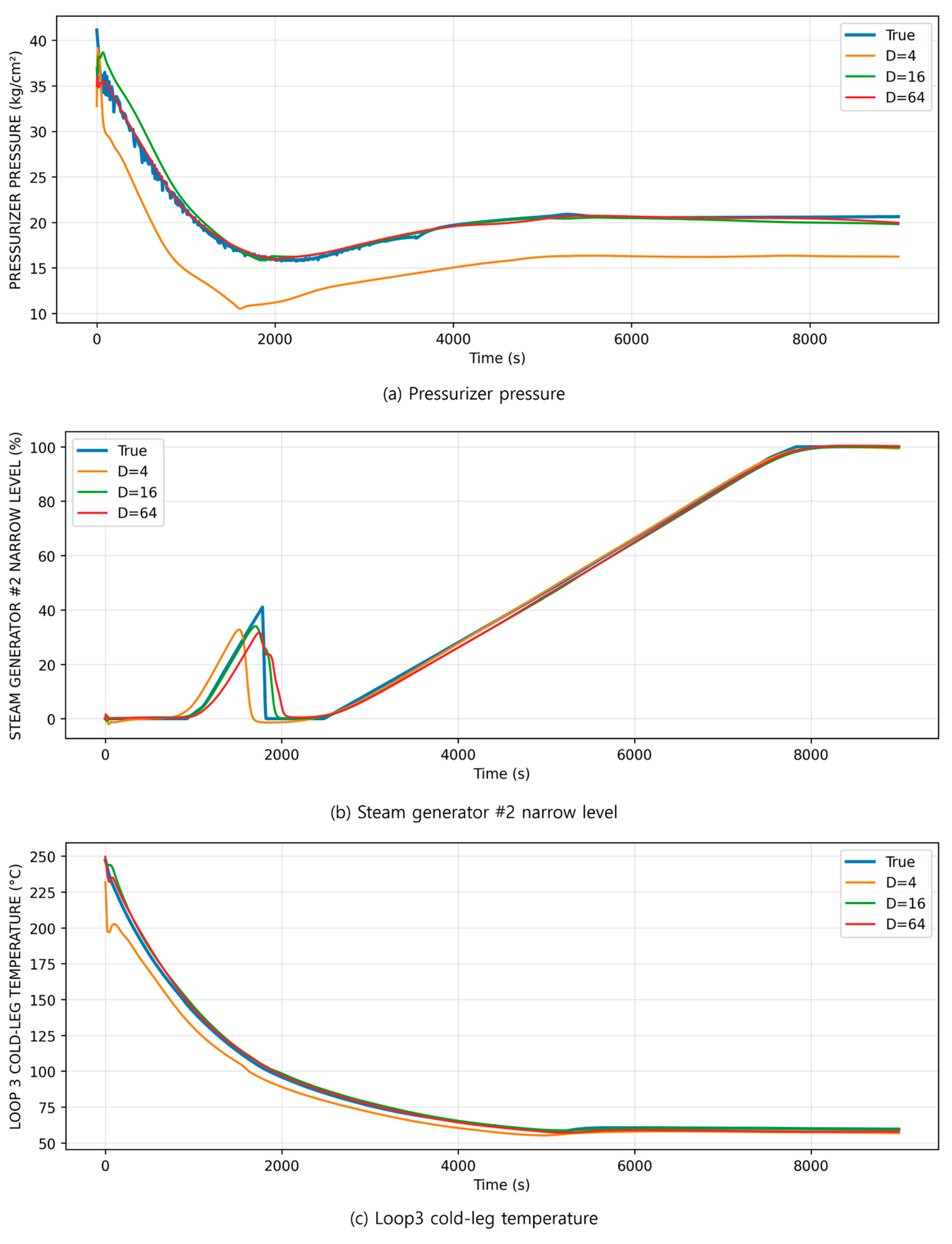
Figure 5 provides a qualitative 25-channel latent-dimension comparison for a held-out LOCA test scenario. The selected case corresponds to LOCA_45_PORVError_1000.csv, in which a 45 cm² break-size LOCA is followed by erroneous PORV opening at 1000 s. Figure 5a shows pressurizer pressure, where D = 4 exhibits a strong low-bias error after the initial depressurization and fails to recover the long-term pressure level. Figure 5b shows steam generator #2 narrow level, where D = 4 and the larger latent dimensions differ mainly in the early transient timing, while all models capture the later level increase. Figure 5c shows loop 3 cold-leg temperature, where D = 4 underestimates the cooling trajectory more strongly than D = 16 and D = 64. Together, these panels support the quantitative z-sweep result by showing that the smallest bottleneck can preserve the broad trend but may lose transient and level information in selected variables.

Figure 5. Qualitative z-sweep comparison in a held-out LOCA scenario.

3.4.3. Reduced-Output Analysis

The reduced-output experiment was then used as a control analysis to test whether lowering the number of predicted variables automatically relaxes the latent-capacity requirement. Table 9 reports the repeated-seed results for the reduced 10-channel task. The reduced-output model remained competitive over a broad range of latent dimensions, but the smallest bottleneck was not uniformly superior. Therefore, the reduced-output task is used here to examine how output scope changes latent-capacity behavior, rather than to claim that reducing the number of variables alone makes the task trivially easier.

Table 9. Latent-dimension sweep in the reduced 10-channel task.

D	MAE	RMSE	DTW	Tolerance-Based Success Rate (%)
4	0.01280 (0.00163)	0.03250 (0.00766)	0.001364 (0.000172)	96.95 (1.15)
8	0.01309 (0.00115)	0.02900 (0.00159)	0.001412 (0.000102)	96.95 (0.92)
16	0.01204 (0.00013)	0.02599 (0.00157)	0.001333 (0.000047)	97.33 (0.16)
24	0.01142 (0.00059)	0.02546 (0.00165)	0.001277 (0.000069)	97.43 (0.57)
32	0.01196 (0.00007)	0.02694 (0.00140)	0.001314 (0.000033)	96.67 (0.44)
48	0.01125 (0.00043)	0.02554 (0.00121)	0.001268 (0.000038)	97.33 (0.44)
64	0.01159 (0.00039)	0.02561 (0.00106)	0.001296 (0.000046)	97.33 (0.59)

Because aggregate comparisons between 25-channel and 10-channel tasks can be affected by the selected variable set, the same-variable control in Table 10 explicitly distinguishes two cases. Reduced10 denotes models trained from the beginning to predict only the reduced set of 10 target variables. Full25→same10 denotes post hoc evaluation of models trained to predict all 25 target variables; from each 25-channel output, only the same 10 reduced target-variable channels were extracted and used for metric calculation. Therefore, Table 10 tests whether training directly on the 10-channel output task provides an advantage over learning the full 25-channel trajectory representation and then evaluating the same 10 variables.

Table 10. Same-variable reduced-output control analysis.

D	Final Forecast RMSE Full25→Same10	Final Forecast RMSE Reduced10	AE Reconstruction RMSE Full25→Same10	AE Reconstruction RMSE Reduced10
4	0.02896 (0.00162)	0.03250 (0.00766)	0.02695 (0.00493)	0.02933 (0.00404)
8	0.03181 (0.00933)	0.02900 (0.00159)	0.02257 (0.00155)	0.02927 (0.00365)
16	0.02685 (0.00065)	0.02599 (0.00157)	0.02224 (0.00160)	0.02701 (0.00337)
24	0.02523 (0.00103)	0.02546 (0.00165)	0.02278 (0.00516)	0.02656 (0.00579)
32	0.02529 (0.00316)	0.02694 (0.00140)	0.01946 (0.00031)	0.02587 (0.00190)
48	0.02545 (0.00125)	0.02554 (0.00121)	0.02586 (0.01005)	0.02542 (0.00167)
64	0.02654 (0.00152)	0.02561 (0.00106)	0.02307 (0.00339)	0.02337 (0.00188)

The same-variable control did not show a uniform advantage for Reduced10. At D = 4, Full25→same10 achieved lower final forecast and AE reconstruction RMSE than Reduced10. Across latent dimensions, the better case alternated for final forecasting, while the full 25-channel AE generally achieved lower reconstruction error when evaluated on the same 10 variables. These results indicate that reducing the number of predicted variables does not automatically reduce the required latent capacity; the effective latent dimension depends on both output scope and the multivariate trajectory structure learned by the model.

To complement normalized aggregate metrics, representative inverse-normalized errors were computed for five plant variables in the H = 1500 horizon-sweep setting. Table 11 reports physical-unit MAE and RMSE for the main direct baseline and the latent model, averaged across the three seeds. These values support operational interpretation by showing the approximate magnitude of errors in plant-variable units.

Table 11. Representative physical-unit errors at H = 1500.

Target variable	Direct MAE	Direct RMSE	Latent MAE	Latent RMSE
Power range (%)	0.174 (0.012)	0.312 (0.023)	0.105 (0.001)	0.203 (0.003)
Core outlet temp (°C)	4.355 (0.179)	6.697 (0.385)	3.710 (0.260)	5.852 (0.528)
Pressurizer pressure (kg/cm2)	2.723 (0.200)	4.026 (0.256)	2.453 (0.150)	3.691 (0.040)
SG 1 narrow level (%)	1.626 (0.053)	2.930 (0.061)	1.023 (0.080)	1.885 (0.203)
Feedwater #1 flow (m3/h)	0.633 (0.201)	1.016 (0.432)	0.516 (0.106)	0.725 (0.171)

Note: Bold values indicate the better mean performance between the direct and latent models for each target variable and error metric. Lower values are better for all reported error metrics.

Across the representative variables, the latent model generally reduced the physical-unit RMSE relative to the main direct baseline at the longest horizon. For example, the mean RMSE decreased from 6.697 °C to 5.852 °C for core outlet temperature and from 2.930% to 1.885% for SG 1 narrow-range level. The exact magnitude varies by variable, but the physical-unit table confirms that the normalized improvements correspond to interpretable changes in plant-parameter units.

3.4.4. Empirical Findings

The experimental results show three consistent patterns after repeated-seed evaluation. First, the advantage of latent trajectory forecasting became clearer as the forecast horizon increased. Second, the 25-channel z sweep showed a broad practical operating range rather than a sharply defined universal optimum, with the smallest tested bottleneck being less reliable in selected dynamic trajectories. Third, the reduced-output control demonstrated that reducing output scope does not automatically make the smallest latent dimension sufficient; same-variable comparisons suggest that latent capacity depends on output scope, selected trajectory structure, and shared multivariate representation.

4. Discussion

The results support a complexity-aware interpretation of long-horizon nuclear plant parameter forecasting. In short-horizon settings, direct observation-space forecasting can remain competitive because the model only needs to estimate a relatively small future trajectory. As the forecast horizon increases, however, the direct model must regress a much larger H × V output object from the same short observation history. The latent formulation reduces this burden by shifting the prediction target from the full trajectory to a compact trajectory-level coordinate, while the decoder provides a learned prior for reconstructing temporally coherent future trajectories. Therefore, the value of latent trajectory forecasting should be understood as scale-dependent rather than universally superior across all forecasting tasks.

This interpretation also clarifies the baseline scope. Models such as Informer, PatchTST, TFT, and TimesFM are important long-sequence forecasting backbones, but the present comparison is not intended to claim superiority over all such architectures. Those models generally improve the sequence-modeling backbone for future time-series extrapolation; whereas, this paper examines a formulation shift from direct observation-space regression to conditional generation of a future trajectory through a learned latent coordinate and decoder. Future work should combine the present latent trajectory formulation with stronger backbone predictors to separate formulation effects from backbone effects more fully.

The latent-dimension experiments further show that the bottleneck size should be interpreted as a task-dependent operating variable rather than as a parameter with a single universal optimum. In the 25-channel, 1500-step task, the smallest tested bottleneck was less favorable on average and in selected trajectory examples, indicating limited representational margin. Once the latent dimension increased beyond this lower-capacity setting, performance entered a broad practical range. This suggests that practical model configuration should focus on balancing compactness, trajectory-level fidelity, robustness, and parameter efficiency rather than selecting a single best D from one metric.

The reduced-output control analysis provides additional insight into the relationship between output scope and latent capacity. Lowering the number of target variables does not simply make the smallest bottleneck sufficient. Same-variable comparisons showed that reduced10 training was competitive for several dimensions, but the full25 representation also remained strong when evaluated on the same 10 variables, especially in autoencoder reconstruction. This suggests that output count is an important design factor, but the required latent capacity is also influenced by trajectory diversity, variable coupling, and the shared multivariate structure learned by the representation model.

These findings have practical implications for AI-assisted plant monitoring and operator-support forecasting. In such applications, model accuracy is important, but so are parameter efficiency, robustness, and ease of configuration. A latent trajectory forecasting framework can provide a useful design direction because it allows the high-dimensional future trajectory to be represented through a compact coordinate system. This may be especially valuable when future operator-support systems need to forecast many plant variables over long time horizons while maintaining a manageable computational footprint. The results also suggest that latent-dimension selection should be treated as part of the model design process, rather than as a purely technical hyperparameter search.

From an application perspective, the proposed framework is most appropriate for operator-support scenarios in which recent plant observations and procedure/action-related signals contain the key conditional information needed to project the future trend. It is less appropriate without further validation for accident families outside the simulator scenario distribution, abrupt unmodeled operator actions, strongly noisy measured plant data, or applications requiring uncertainty bounds rather than deterministic point forecasts. These applicability boundaries should be considered when interpreting the reported quantitative improvements.

At the same time, the findings should not be overgeneralized. This study used simulator-derived CNS data with a fixed scenario-file split and focused on deterministic point forecasts. The repeated-seed results reduce the concern that the reported trends arise from a single favorable run, but additional scenario splits, accident families, and forecasting backbones are still needed to assess broader generality. The inverse-normalized physical-unit errors provide an operational interpretation for representative plant variables, but deployment-oriented validation should also examine measurement noise, missing data, and uncertainty quantification.

Future work should therefore examine whether the observed latent-scaling behavior remains stable across different scenario splits, additional accident types, and alternative forecasting architectures. Incorporating uncertainty quantification would also be important for operator-support applications, where confidence information can be as important as point prediction accuracy. Another useful extension would be to investigate adaptive or variable-specific latent representations, because different plant variables may require different levels of representational capacity depending on their transient behavior and coupling with other variables.

5. Conclusions

This study investigated long-horizon multivariate forecasting of nuclear power plant parameters from short observation histories. The forecasting problem was formulated as a trajectory-scaling problem in which the output dimension grows with both the forecast horizon and the number of target variables. To address this scaling issue, direct observation-space forecasting was compared with an LSTM autoencoder-based latent trajectory forecasting framework.

The repeated-seed horizon-sweep results showed that direct forecasting remained competitive in short-horizon settings; whereas, latent trajectory forecasting became increasingly advantageous as the forecast horizon increased within the direct LSTM baseline comparison considered in this study. In the longest-horizon task, the latent framework achieved lower prediction error while using substantially fewer parameters than the direct LSTM baselines. The smaller direct LSTM baseline further suggested that the advantage of the latent formulation cannot be explained by parameter-count reduction alone; rather, forecasting in a compact trajectory representation space provides a structural alternative to direct full-trajectory regression.

The repeated-seed latent-dimension analyses further showed that performance did not depend on a single sharply optimal latent dimension. The 25-channel task exhibited a broad practical range across moderate-to-large D values, while qualitative examples showed that the smallest tested bottleneck can be less reliable for selected dynamic trajectories. The reduced-output control analysis further indicated that output-variable count alone does not determine latent-capacity requirements, reinforcing the view that latent dimension should be treated as a task-dependent configuration variable.

Overall, the findings support the use of latent trajectory forecasting as a practical design direction for AI-assisted nuclear plant monitoring and operator-support systems. Rather than directly regressing large future trajectories in the observation space, long-horizon forecasting models can benefit from learning compact trajectory-level representations. The additional physical-unit analysis helps connect normalized aggregate metrics to operationally interpretable plant-variable errors. Future work should examine the robustness of this scaling behavior across broader accident scenarios, alternative architectures, and uncertainty-aware forecasting frameworks.

References

- Bae, J.; Kim, G.; Lee, S.J. Real-time prediction of nuclear power plant parameter trends following operator actions. Expert Syst. Appl. 2021, 186, 115848. [Google Scholar] [CrossRef] [Scilit]
- Bae, J.; Kim, K.S.; Lee, S.J. Two-stage deep learning model for nuclear power plant parameter trend prediction with epistemic uncertainty quantification. Appl. Soft Comput. 2026, 186, 114233. [Google Scholar] [CrossRef] [Scilit]
- Radaideh, M.I.; Pigg, C.; Kozlowski, T.; Deng, Y.; Qu, A. Neural-based time series forecasting of loss of coolant accidents in nuclear power plants. Expert Syst. Appl. 2020, 160, 113699. [Google Scholar] [CrossRef] [Scilit]
- Nguyen, H.-P.; Liu, J.; Zio, E. A long-term prediction approach based on long short-term memory neural networks with automatic parameter optimization by Tree-structured Parzen Estimator and applied to time-series data of NPP steam generators. Appl. Soft Comput. 2020, 89, 106116. [Google Scholar] [CrossRef] [Scilit]
- Kim, H.; Kim, J. Long-term prediction of safety parameters with uncertainty estimation in emergency situations at nuclear power plants. Nucl. Eng. Technol. 2023, 55, 1630–1643. [Google Scholar] [CrossRef] [Scilit]
- Wapachi, F.I.; Diab, A. Time-series forecasting of a typical PWR system response under control element assembly withdrawal at full power. Nucl. Eng. Des. 2023, 413, 112472. [Google Scholar] [CrossRef] [Scilit]
- Nguyen, T.C.H.; Diab, A. Using machine learning to forecast and assess the uncertainty in the response of a typical PWR undergoing a steam generator tube rupture accident. Nucl. Eng. Technol. 2023, 55, 3423–3440. [Google Scholar] [CrossRef] [Scilit]
- Lee, Y.; Song, S.H.; Bae, J.Y.; Song, K.; Seo, M.R.; Kim, S.J.; Lee, J.I. Surrogate model for predicting severe accident progression in nuclear power plant using deep learning methods and rolling-window forecast. Ann. Nucl. Energy 2024, 208, 110816. [Google Scholar] [CrossRef] [Scilit]
- Xiao, X.; Song, M.; Liu, X. A reliable and adaptive prediction framework for nuclear power plant system through an improved Transformer model and Bayesian uncertainty analysis. Reliab. Eng. Syst. Saf. 2025, 261, 111076. [Google Scholar] [CrossRef] [Scilit]
- Kim, M.S.; Na, M.G. Multivariate prediction of major safety variables with confidence estimation during severe accidents in nuclear power plants. Nucl. Eng. Technol. 2026, 58, 103996. [Google Scholar] [CrossRef] [Scilit]
- Ma, M.; Zhang, H.; Du, L.; Zhao, M.; Yang, Y. Application of neural networks for fast prediction of key safety parameters in nuclear power plant transients. Ann. Nucl. Energy 2026, 227, 111935. [Google Scholar] [CrossRef] [Scilit]
- Ben Taieb, S.; Bontempi, G.; Atiya, A.F.; Sorjamaa, A. A review and comparison of strategies for multi-step ahead time series forecasting based on the NN5 forecasting competition. Expert Syst. Appl. 2012, 39, 7067–7083. [Google Scholar] [CrossRef] [Scilit]
- Sorjamaa, A.; Hao, J.; Reyhani, N.; Ji, Y.; Lendasse, A. Methodology for long-term prediction of time series. Neurocomputing 2007, 70, 2861–2869. [Google Scholar] [CrossRef] [Scilit]
- Zhou, H.; Zhang, S.; Peng, J.; Zhang, S.; Li, J.; Xiong, H.; Zhang, W. Informer: Beyond efficient Transformer for long sequence time-series forecasting. arXiv 2020, arXiv:2012.07436. [Google Scholar]
- Lim, B.; Arık, S.Ö.; Loeff, N.; Pfister, T. Temporal Fusion Transformers for interpretable multi-horizon time series forecasting. Int. J. Forecast. 2021, 37, 1748–1764. [Google Scholar] [CrossRef] [Scilit]
- Nguyen, N.; Quanz, B. Temporal latent auto-encoder: A method for probabilistic multivariate time series forecasting. arXiv 2021, arXiv:2101.10460. [Google Scholar]
- Cai, B.; Yang, S.; Gao, L.; Xiang, Y. Hybrid variational autoencoder for time series forecasting. Knowl.-Based Syst. 2023, 281, 111079. [Google Scholar] [CrossRef] [Scilit]
- Solera-Rico, A.; Sanmiguel Vila, C.; Gómez, M.A.; Wang, Y.; Almashjary, A.; Dawson, S.T.M.; Vinuesa, R. β-Variational autoencoders and transformers for reduced-order modelling of fluid flows. arXiv 2023, arXiv:2304.03571. [Google Scholar]
- Nayak, I.; Chakrabarty, A.; Kumar, M.; Teixeira, F.; Goswami, D. Temporally-consistent Koopman autoencoders for forecasting dynamical systems. arXiv 2024, arXiv:2403.12335. [Google Scholar]
- Franco, N.R.; Fraulin, D.; Manzoni, A.; Zunino, P. On the latent dimension of deep autoencoders for reduced order modeling of PDEs parametrized by random fields. arXiv 2023, arXiv:2310.12095. [Google Scholar]
- Song, H.; Liu, X.; Song, M. Comparative study of data-driven and model-driven approaches in prediction of nuclear power plants operating parameters. Appl. Energy 2023, 341, 121077. [Google Scholar] [CrossRef] [Scilit]
- Song, H.; Song, M.; Liu, X. Online autonomous calibration of digital twins using machine learning with application to nuclear power plants. Appl. Energy 2022, 326, 119995. [Google Scholar] [CrossRef] [Scilit]
- Nie, Y.; Nguyen, N.H.; Sinthong, P.; Kalagnanam, J. A Time Series is Worth 64 Words: Long-term Forecasting with Transformers. International Conference on Learning Representations (ICLR). arXiv 2023, arXiv:2211.14730. [Google Scholar]
- Das, A.; Kong, W.; Sen, R.; Zhou, Y. A decoder-only foundation model for time-series forecasting. In Proceedings of the 41st International Conference on Machine Learning (ICML), Vienna, Austria, 21–27 July 2024. [Google Scholar] [CrossRef] [Scilit]
- Rombach, R.; Blattmann, A.; Lorenz, D.; Esser, P.; Ommer, B. High-Resolution Image Synthesis with Latent Diffusion Models. In Proceedings of the IEEE/CVF Conference on Computer Vision and Pattern Recognition (CVPR), New Orleans, LA, USA, 18–24 June 2022; pp. 10684–10695. [Google Scholar]
- Gao, Z.; Shi, X.; Han, B.; Wang, H.; Jin, X.; Maddix, D.; Zhu, Y.; Li, M.; Wang, Y. PreDiff: Precipitation Nowcasting with Latent Diffusion Models. Advances in Neural Information Processing Systems 36 (NeurIPS). arXiv 2023, arXiv:2307.10422. [Google Scholar]
- Zhuang, Y.; Duraisamy, K. LaDCast: A Latent Diffusion Model for Medium-Range Ensemble Weather Forecasting. arXiv 2025, arXiv:2506.09193. [Google Scholar] [CrossRef] [Scilit]
- Kontolati, K.; Goswami, S.; Karniadakis, G.E.; Shields, M.D. Learning nonlinear operators in latent spaces for real-time predictions of complex dynamics in physical systems. Nat. Commun. 2024, 15, 5101. [Google Scholar] [CrossRef] [Scilit] [PubMed]
- Li, Z.; Patil, S.; Ogoke, F.; Shu, D.; Zhen, W.; Schneier, M.; Buchanan, J.R., Jr.; Farimani, A.B. Latent Neural PDE Solver: A reduced-order modelling framework for partial differential equations. arXiv 2024, arXiv:2402.17853. [Google Scholar] [CrossRef] [Scilit]
Disclaimer/Publisher’s Note: The statements, opinions and data contained in all publications are solely those of the individual author(s) and contributor(s) and not of MDPI and/or the editor(s). MDPI and/or the editor(s) disclaim responsibility for any injury to people or property resulting from any ideas, methods, instructions or products referred to in the content. |
© 2026 by the authors. Licensee MDPI, Basel, Switzerland. This article is an open access article distributed under the terms and conditions of the Creative Commons Attribution (CC BY) license.