A Hybrid Radial Basis Function–Finite Difference Matrix Operators (RBF–FDMO) Approach for Numerical Simulation of Grounding Systems on Non-Uniform FD Mesh

Abstract

This paper presents a hybrid numerical approach, termed the Radial Basis Function–Finite Difference Matrix Operator (RBF–FDMO) method, to enhance the accuracy and flexibility of the conventional FDMO technique for three-dimensional (3D) electromagnetic field analysis governed by the Laplace–Poisson equation. Conventional numerical methods often face challenges related to computational complexity and limited flexibility when handling non-uniform discretization and complex geometries. In the proposed method, spatial derivatives are approximated using RBF-based interpolation rather than finite difference schemes derived from Taylor series expansion. This formulation enables the construction of high-accuracy derivative operators on both uniform and non-uniform FD grids, thereby improving numerical robustness and adaptability to complex geometries. The performance of the proposed method is first compared with the FDMO in a 3D benchmark problem, with reductions of more than two orders of magnitude in both RMS and maximum errors. Furthermore, the RBF-FDMO approach is developed and, for the first time, applied to the analysis of grounding system (GS) configurations specified in IEEE Std. 80™, as well as a practical 110 kV substation GS in Vietnam. The obtained potential distributions, grounding resistances, and touch and step voltages confirm the effectiveness and reliability of the method. The results indicate that the proposed approach features a simple formulation and competitive computational efficiency, positioning it as a practical alternative to conventional methods like the finite element method (FEM) and the boundary element method (BEM) for GS analysis and design.

1. Introduction

The GS is one of the key components in the design and operation of power systems. It performs three primary functions, including system operational grounding, equipment protective grounding, and lightning protection grounding. When faults occur in power systems, such as insulation breakdowns, short circuits to ground, or lightning discharges, the GS provides a low-impedance path for fault and surge currents to flow into the earth. As a result, the GS not only ensures the effective operation of protection devices but also upholds personnel safety and contributes to the electromagnetic compatibility and stability of entire power systems [1,2,3].

In the case of protective grounding, this problem is commonly described by the 3D Laplace equation:

$${\nabla }^2\phi =0,$$

(1)

where $\phi$ denotes the electric potential.

Accurate solutions to the Laplace equation allow for the assessment of key safety parameters, such as earth resistance, touch voltage, and step voltage, which are critical for ensuring compliance with national and international standards, including IEEE Std. 80™ [1,4].

The analysis of a complex GS, characterized by irregular geometries and non-homogeneous soil conditions, often requires the use of advanced numerical methods to obtain reliable and accurate results. Among the available numerical methods, the FEM stands out as a robust and flexible approach, capable of delivering high accuracy when dealing with complex three-dimensional regions characterized by spatially varying material properties [5,6,7]. By discretizing the entire computational domain into a large number of finite elements, FEM transforms the governing Laplace equation into a system of algebraic equations. However, this volumetric discretization results in a substantial number of unknowns, leading to large sparse matrices that demand significant computational resources and memory [8,9]. Furthermore, the mesh generation process is often cumbersome for a GS featuring numerous buried conductors and multilayer soil structures. The necessity of accurately representing the infinite soil domain using artificial boundaries also introduces modeling uncertainty, as the choice of boundary distance and type can notably affect the solution accuracy. Consequently, FEM-based GS analysis becomes time-consuming and computationally expensive, especially when dealing with large substations or parameter sweeps.

Complementing the FEM, the BEM has gained considerable attention owing to its ability to reduce the problem dimensionality and computational cost [10,11,12,13]. Unlike the FEM, the BEM requires discretization only along the boundaries of the problem domain, which considerably reduces the number of elements and simplifies the representation of open-boundary problems. Despite these advantages, the BEM is less efficient when handling non-homogeneous or multilayer soils, as the derivation of suitable Green’s functions becomes mathematically complex and the resulting system matrices are often ill-conditioned. Additionally, for large or highly interconnected GS configurations, the dense and fully populated matrices inherent to the BEM can lead to increased memory requirements and longer computation times.

To overcome the limitations of each approach, the hybrid FEM–BEM technique has been proposed [14]. In this formulation, the FEM efficiently captures the volumetric complexity within the soil, while the BEM accurately models the behavior at infinity, thereby improving overall accuracy. However, this hybridization increases the implementation complexity, as it requires coupling of two distinct formulations and exchanging of boundary information at their interface. Such procedures often entail additional pre- and post-processing steps, making the hybrid approach less straightforward for large-scale or iterative GS studies.

Another widely used approach is the method of moment (MoM), which reformulates the potential distribution problem into an integral-equation framework [15]. The MoM is well suited for thin-wire models of grounding conductors, with emphasis on the evaluation of longitudinal current distribution. Nonetheless, its application to extensive GS models is limited due to the rapid growth of the dense impedance matrix, which scales quadratically with the number of segments. Moreover, MoM assumes simplified soil models and faces challenges when incorporating realistic multilayer or frequency-dependent soil characteristics. These factors collectively increase computational cost and reduce modeling flexibility.

Overall, while the FEM, BEM, and MoM have proven to be robust and accurate in specific applications, their inherent drawbacks—complex meshing, high computational demand, and limited adaptability to non-uniform soils—highlight the need for a more efficient and flexible numerical framework for realistic GS analysis. Despite their effectiveness, conventional numerical methods for grounding system analysis face several mathematical and computational challenges. These include the requirement for fine and structured meshing to maintain numerical stability, the generation of large sparse or dense matrix systems that impose significant memory and processing demands, and limited flexibility in handling irregular geometries or highly heterogeneous soil profiles.

For grounding-system analysis, the comparison among numerical methods in this study is primarily focused on aspects that are most relevant to the present problem, namely formulation simplicity, flexibility for non-uniform discretization, and applicability to practical grounding-grid modeling. From this perspective, although FEM, BEM, and MoM are well-established and effective in many applications, their limitations motivate the development of alternative approaches that can retain numerical accuracy while offering a more straightforward operator-based formulation.

Accordingly, the main novelty of the present work lies in integrating RBF-based derivative approximation into the classical FDMO framework for three-dimensional grounding-system analysis. Unlike the Taylor-series-based derivative construction used in the conventional FDMO formulation, the proposed hybrid RBF-FDMO approach enables more flexible and accurate operator construction on both uniform and non-uniform grids, thereby extending the applicability of the FDMO method to grounding-system modeling.

Motivated by these considerations, the finite difference method (FDM)—with its mathematically simple approach, competitive computational efficiency, and high applicability—has been employed for the simulation of GS [16,17]. In this work, we present, for the first time, the RBF-FDMO method, which integrates the 3D FDMO approach proposed in [17] with the use of RBF approximations to the GS analysis. First, we developed the RBF-FDMO method in 3-D domain and validated it by solving a benchmark 3-D problem. The method is then combined with a non-uniform FD mesh, enabling improved flexibility and accuracy when modeling GS with complex geometries. This combined approach is applied to simulate several GS configurations defined in IEEE Std. 80™ and the GS of the 110 kV high-voltage substation in Vietnam. The obtained results demonstrate that the RBF-FDMO method consistently delivers more accurate solutions compared to conventional methods such as the BEM, FEM, and the procedures outlined in IEEE Std. 80™.

The main contributions of this study can be summarized as follows:

• A novel hybrid method integrating RBFs with the FDMO approach has been successfully developed, resulting in the RBF-FDMO method. This combination not only achieves significantly higher solution accuracy than the original FDMO proposed in 3-D domain [17], but also provides greater flexibility in handling complex geometries and both uniform and non-uniform grids through the use of RBF interpolation.
• This study marks the initial use of the RBF-FDMO technique in simulating and evaluating both theoretical and practical GSs. In particular, the 3-D finite difference grid employed in this work is non-uniform, and its effectiveness has been validated in [18,19]. The approach provides accuracy equivalent to well-known methods such as the FEM and BEM, while benefiting from a more straightforward mathematical framework and simpler implementation.

The structure of this paper is outlined as follows: In Section 2, we formulate the RBF-FDMO approximations for the 3-D EMF problem. Section 3 briefly presents the algorithm for determining the optimal shape parameter proposed by Victor Bayona et al. in [20]. Section 4 presents our study’s findings, where the RBF–FDMO method is applied to analysis potential distribution, earth resistance, touch and step voltages of several benchmark and real-world GSs. Finally, Section 4 provides remarks and conclusions of the paper.

2. Hybrid RBF-FDMO Method for Solving Poisson–Laplace Equations

In Cartesian coordinates, the 3-D Poisson–Laplace equation can be expressed as

$${\nabla }^{2}u(x,y,z)=f(x,y,z),x,y,z\in \Omega ,$$

(2)

The Laplacian in (2) is written in Cartesian coordinates as

$${\nabla }^{2}u(x,y,z)={\displaystyle \frac{{\partial }^{2}u(x,y,z)}{\partial x^2}}+{\displaystyle \frac{{\partial }^{2}u(x,y,z)}{\partial y^2}}+{\displaystyle \frac{{\partial }^{2}u(x,y,z)}{\partial z^2}},$$

(3)

and $\Omega$ is the solution domain.

This section develops an RBF-FDMO formulation by extending the FDMO approach in [17,21] and incorporating GA, MQ, IQ, and IMQ RBFs, following [22]. The specific RBF forms employed in this study are detailed in Table 1. This approach is formulated to solve the benchmark 3-D EMF problem with improved accuracy and stability. This development aims to broaden the RBF-FDMO method’s applicability for computing potential distributions of GS in 3-D domains.

Table 1. List of employed radial basis functions (RBFs).

RBF Type	Definition
Gaussian (GA)	$e^{-{(r/c)}^2}$
Multiquadric (MQ)	$\sqrt{r^2+c^2}$
Inverse Quadratic (IQ)	${\displaystyle \frac{1}{r^2+c^2}}$
Inverse Multiquadric (IMQ)	${\displaystyle \frac{1}{\sqrt{r^2+c^2}}}$

Note: $r={\parallel \mathit{x}-{\mathit{x}}_j\parallel }_2$, where $c>0$ is the shape parameter.

2.1. RBF-FDMO Formulation for 1-D Poisson Equation

For a problem involving only one spatial variable x, the three-dimensional formulation in (2) reduces to

$${\displaystyle \frac{d^{2}u\left(x\right)}{d{x}^2}}=f\left(x\right),x\in \Omega ,$$

(4)

where the computational domain is denoted by $\Omega =[x_1,x_N]$ and its boundary is given by $\Gamma =\{x_1,x_N\}$.

By applying central-difference expressions to the radial basis function expansion, one can derive the corresponding RBF-based formulas for the first- and second-order spatial derivatives; see, for example, [22,23].

$${\displaystyle \frac{du}{dx}}{|}_{x=x_i}\approx u_i^{\prime }={\alpha }_1{u}_{i-1}+{\alpha }_2{u}_i+{\alpha }_3{u}_{i+1},$$

(5)

$${\displaystyle \frac{d^{2}u}{d{x}^2}}{|}_{x=x_i}\approx u_i^{\prime }={\beta }_1{u}_{i-1}+{\beta }_2{u}_i+{\beta }_3{u}_{i+1}.$$

(6)

Equations (5) and (6) can be written into a matrix form as

$$u_i^{\prime }=\left[\begin{array}{ccc}{\alpha }_1& {\alpha }_2& {\alpha }_3\end{array}\right]·\left[\begin{array}{c}{u}_{i-1}\\ u_i\\ u_{i+1}\end{array}\right],$$

(7)

$$u_i^{″}=\left[\begin{array}{ccc}{\beta }_1& {\beta }_2& {\beta }_3\end{array}\right]·\left[\begin{array}{c}{u}_{i-1}\\ u_i\\ u_{i+1}\end{array}\right].$$

(8)

Equations (7) and (8) are formulated for the interior nodes of the grid, i.e., for $i=2$ through $N-1$. At the two boundary nodes, $i=1$ and $i=N$, these expressions would require the values $u_0$ and $u_{N+1}$, which are not part of the computational domain. Consequently, the interior scheme cannot be applied directly at the boundaries. To obtain the required derivative approximations, a forward RBF discretization is used at $i=1$, and a backward RBF discretization is employed at $i=N$. The corresponding formulas are presented below.

The forward RBF approximation is

$$u_1^{\prime }=\left[\begin{array}{ccc}{\alpha }_{1F}& {\alpha }_{2F}& {\alpha }_{3F}\end{array}\right]·{\left[\begin{array}{ccc}{u}_1& u_2& u_3\end{array}\right]}^T,$$

(9)

$$u_1^{″}=\left[\begin{array}{ccc}{\beta }_{1F}& {\beta }_{2F}& {\beta }_{3F}\end{array}\right]·{\left[\begin{array}{ccc}{u}_1& u_2& u_3\end{array}\right]}^T,$$

(10)

and the backward RBF approximation is

$$u_N^{\prime }=\left[\begin{array}{ccc}{\alpha }_{3B}& {\alpha }_{2B}& {\alpha }_{1B}\end{array}\right]·{\left[\begin{array}{ccc}{u}_{N-2}& u_{N-1}& u_N\end{array}\right]}^T,$$

(11)

$$u_N^{″}=\left[\begin{array}{ccc}{\beta }_{3B}& {\beta }_{2B}& {\beta }_{1B}\end{array}\right]·{\left[\begin{array}{ccc}{u}_{N-2}& u_{N-1}& u_N\end{array}\right]}^T,$$

(12)

in which these weighting coefficients of $\left({\alpha }^{GA},{\beta }^{GA}\right)$, $\left({\alpha }^{MQ},{\beta }^{MQ}\right)$, $\left({\alpha }^{IQ},{\beta }^{IQ}\right)$, and $\left({\alpha }^{IMQ},{\beta }^{IMQ}\right)$ are derived in Appendix A.

Assembling (9)–(12) for all i yields the matrix forms in (13) and (14).

$$\left[\begin{array}{c}{u}_1^{\prime }\\ u_2^{\prime }\\ u_3^{\prime }\\ ⋮\\ u_{N-1}^{\prime }\\ u_N^{\prime }\end{array}\right]=\underset{D_{\alpha }^{1D}}{\underbrace{\left[\begin{array}{ccccccccc}{\alpha }_{1F}& {\alpha }_{2F}& {\alpha }_{3F}& 0& \dots & 0& 0& 0& 0\\ {\alpha }_1& {\alpha }_2& {\alpha }_3& 0& \dots & 0& 0& 0& 0\\ 0& {\alpha }_1& {\alpha }_2& {\alpha }_3& \dots & 0& 0& 0& 0\\ ⋮& ⋮& ⋮& ⋮& \ddots & ⋮& ⋮& ⋮& ⋮\\ 0& 0& 0& 0& \dots & 0& {\alpha }_1& {\alpha }_2& {\alpha }_3\\ 0& 0& 0& 0& \dots & 0& {\alpha }_{3B}& {\alpha }_{2B}& {\alpha }_{1B}\end{array}\right]}}·\left[\begin{array}{c}{u}_1\\ u_2\\ u_3\\ ⋮\\ u_{N-1}\\ u_N\end{array}\right]$$

(13)

$$\left[\begin{array}{c}{u}_1^{″}\\ u_2^{″}\\ u_3^{″}\\ ⋮\\ u_{N-1}^{″}\\ u_N^{″}\end{array}\right]=\underset{D_{\beta }^{1D}}{\underbrace{\left[\begin{array}{ccccccccc}{\beta }_{1F}& {\beta }_{2F}& {\beta }_{3F}& 0& \dots & 0& 0& 0& 0\\ {\beta }_1& {\beta }_2& {\beta }_3& 0& \dots & 0& 0& 0& 0\\ 0& {\beta }_1& {\beta }_2& {\beta }_3& \dots & 0& 0& 0& 0\\ ⋮& ⋮& ⋮& ⋮& \ddots & ⋮& ⋮& ⋮& ⋮\\ 0& 0& 0& 0& \dots & 0& {\beta }_1& {\beta }_2& {\beta }_3\\ 0& 0& 0& 0& \dots & 0& {\beta }_{3B}& {\beta }_{2B}& {\beta }_{1B}\end{array}\right]}}\left[\begin{array}{c}{u}_1\\ u_2\\ u_3\\ ⋮\\ u_{N-1}\\ u_N\end{array}\right]$$

(14)

For a non-uniform FD mesh, the coefficients $D_{\alpha }^{1D}$ and $D_{\beta }^{1D}$ vary from one interval to another rather than remaining constant. As a result, the usual uniform-mesh terms $D_{\alpha }^{1D}$ and $D_{\beta }^{1D}$ in the differentiation matrices must be replaced by local coefficients that account for the actual spacing between adjacent nodes. Incorporating these position-dependent factors yields the following algebraic matrix expressions for the derivative operators:

$${\mathbf{u}}^{\prime }=D_{\alpha }^{1D}\mathbf{u},$$

(15)

$${\mathbf{u}}^{″}=D_{\beta }^{1D}\mathbf{u}.$$

(16)

In this formulation, $D_{\alpha }^{1D}$ and $D_{\beta }^{1D}$ denote the $N\times N$ differentiation matrices introduced in (13) and (14). When applied to a vector of nodal values, these matrices provide the discrete approximations of the first- and second-order spatial derivatives. Using these operators, the differential equation in (4) can be rewritten in the form of a linear algebraic system.

$$\mathcal{L}\mathbf{u}=\left\{\begin{array}{cc}\mathbf{f},\hfill & \mathrm{in}\Omega ,\hfill \\ \mathbf{g},\hfill & \mathrm{on}\Gamma ,\hfill \end{array}\right.$$

(17)

where the system matrix takes the form

$$\mathcal{L}=\left\{\begin{array}{c}{D}_{\beta }^{1D},\mathrm{in}\Omega ,\hfill \\ B^{1D},\mathrm{on}\Gamma \hfill \end{array}\right.,$$

(18)

and the boundary operator takes the form

$$B^{1D}=\left\{\begin{array}{c}{I}_N,\mathrm{for}\mathrm{Dirichlet}\mathrm{boundary}\hfill \\ D_{\alpha }^{1D},\mathrm{for}\mathrm{Neumann}\mathrm{boundary}\hfill \end{array}\right..$$

(19)

where $I_N$ is the $N\times N$ identity matrix.

2.2. RBF-FDMO Formulation for 3-D Poisson Equation

Here, the Kronecker-product formulation used for two matrices in the 2-D case [21] is generalized to a three-matrix Kronecker structure suitable for the 3-D Poisson–Laplace equation of (2) as presented in [17]. With this extension, the one-dimensional operators $D_{\alpha }^{1D}$ and $D_{\beta }^{1D}$ introduced in (13) and (14) are incorporated into the 3-D setting as

$$D_{{\alpha }_x}^{3D}=I_{N_z}\otimes (I_{N_y}\otimes D_{{\alpha }_x}^{1D}),$$

(20)

$$D_{{\alpha }_y}^{3D}=I_{N_z}\otimes (D_{{\alpha }_y}^{1D}\otimes I_{N_x}),$$

(21)

$$D_{{\alpha }_z}^{3D}=D_{{\alpha }_z}^{1D}\otimes (D_{{\alpha }_y}^{1D}\otimes I_{N_x}),$$

(22)

and

$$D_{{\beta }_x}^{3D}=I_{N_z}\otimes (I_{N_y}\otimes D_{{\beta }_x}^{1D}),$$

(23)

$$D_{{\beta }_y}^{3D}=I_{N_z}\otimes (D_{{\beta }_y}^{1D}\otimes I_{N_x}),$$

(24)

$$D_{{\beta }_z}^{3D}=D_{{\beta }_z}^{1D}\otimes (D_{{\alpha }_y}^{1D}\otimes I_{N_x}),$$

(25)

By substituting the relations in (20)–(25) into the three-dimensional formulation, the expressions given in (18) and (19) can be recast into the following form:

$$\mathcal{L}=\left\{\begin{array}{c}{D}_{{\beta }_x}^{3D}+D_{{\beta }_y}^{3D}+D_{{\beta }_z}^{3D},\mathrm{in}\Omega ,\hfill \\ B^{3D},\mathrm{on}\Gamma \hfill \end{array}\right. ,$$

(26)

and the operator for the boundary conditions is defined as follows:

$$B^{3D}=\left\{\begin{array}{c}{I}_{N_x{N}_y{N}_z},\mathrm{for}\mathrm{Dirichlet}\mathrm{boundary}\hfill \\ D_{{\alpha }_x}^{3D}\mathrm{or}{D}_{{\alpha }_y}^{3D}\mathrm{or}{D}_{{\alpha }_z}^{3D}\mathrm{for}\mathrm{Neumann}\mathrm{boundary}\hfill \end{array}\right. ,$$

(27)

where $I_{N_x{N}_y{N}_z}$ is an identity matrix of size $N_x{N}_y{N}_z\times N_x{N}_y{N}_z$.

In the grounding-system application considered in this study, the far-field truncation boundary is treated as a Dirichlet boundary, $\varphi =0$, whereas the earth surface is modeled as a homogeneous Neumann boundary, $\partial \varphi /\partial n=0$. This row-replacement procedure yields a single global algebraic system that can be solved in a unified manner for both interior and boundary nodes.

3. Choosing Optimal Shape Parameters of the RBFs

The optimal shape parameters of RBFs can be determined by various approaches, as discussed in [24]. In this work, we utilize the algorithm for selecting the optimal shape parameter, as proposed by Victor Bayona et al. [20], and adapt it to our RBFs. This approach, which aims to enhance the accuracy and efficiency of RBF interpolation, is detailed as follows.

Consider a one-dimensional domain discretized into N scattered points, where $NI$ represents the total number of interior points within the domain. Consequently, the difference $N-NI$ corresponds to the two boundary points.

The RBF-FDMO error is given by

$$\mathbf{E}\left(\epsilon \right)=\mathbf{u}-\widehat{\mathbf{u}}\left(\epsilon \right),$$

(28)

where $\widehat{\mathbf{u}}=[\widehat{u}(x_1,\epsilon ),$…$,\widehat{u}(x_N,\epsilon ){]}^{\mathrm{T}}$ is the RBF-FDMO approximation and $\mathbf{u}=[u\left(x_1\right),$…$,u\left(x_N\right){]}^{\mathrm{T}}$ is the exact solution.

In order to find the “optimal” value of the shape parameter $\epsilon *$, the approximation error $\mathbf{E}\left(\epsilon \right)$, as defined in (28), is minimized. This is achieved through the following expression, which allows for an efficient determination of $\epsilon *$ that results in the best possible approximation:

$${\parallel \mathbf{E}(\epsilon *)\parallel }_{\infty }=\underset{\epsilon }{min}{\parallel \mathbf{u}-\widehat{\mathbf{u}}\left(\epsilon \right)\parallel }_{\infty }.$$

(29)

4. Numerical Results

4.1. Application of the RBF-FDMO Method to the 3-D Benchmark Problem

Consider the following 3-D Poisson equation, as discussed in [25], which forms the basis for many engineering and physics problems. In this context, the equation relates the scalar potential field, typically denoted as $u(x,y,z)$, to the spatial distribution of a source function, $g(x,y,z)$, which can represent charge density in electrostatics or mass distribution in gravitation problems. The solution to this equation provides a model for the potential field generated by the sources, allowing for the analysis and prediction of physical behavior in various applications.

$$\left\{\begin{array}{c}{\displaystyle \frac{{\partial }^{2}u}{\partial x^2}}+{\displaystyle \frac{{\partial }^{2}u}{\partial y^2}}+{\displaystyle \frac{{\partial }^{2}u}{\partial z^2}}=sin\left(\pi x\right)sin\left(\pi y\right)sin\left(\pi z\right),x,y,z\in \Omega ,\hfill \\ u(x,y,z)=0,x,y,z\in \partial \Omega ,\hfill \end{array}\right.$$

(30)

where $\Omega =[0,1]\times [0,1]\times [0,1]$. The exact solution is given by

$$u(x,y,z)=-{\displaystyle \frac{1}{3{\pi }^2}}sin\left(\pi x\right)sin\left(\pi y\right)sin\left(\pi z\right).$$

(31)

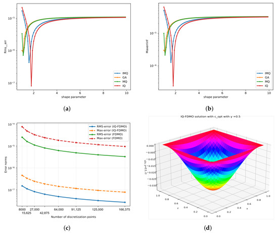
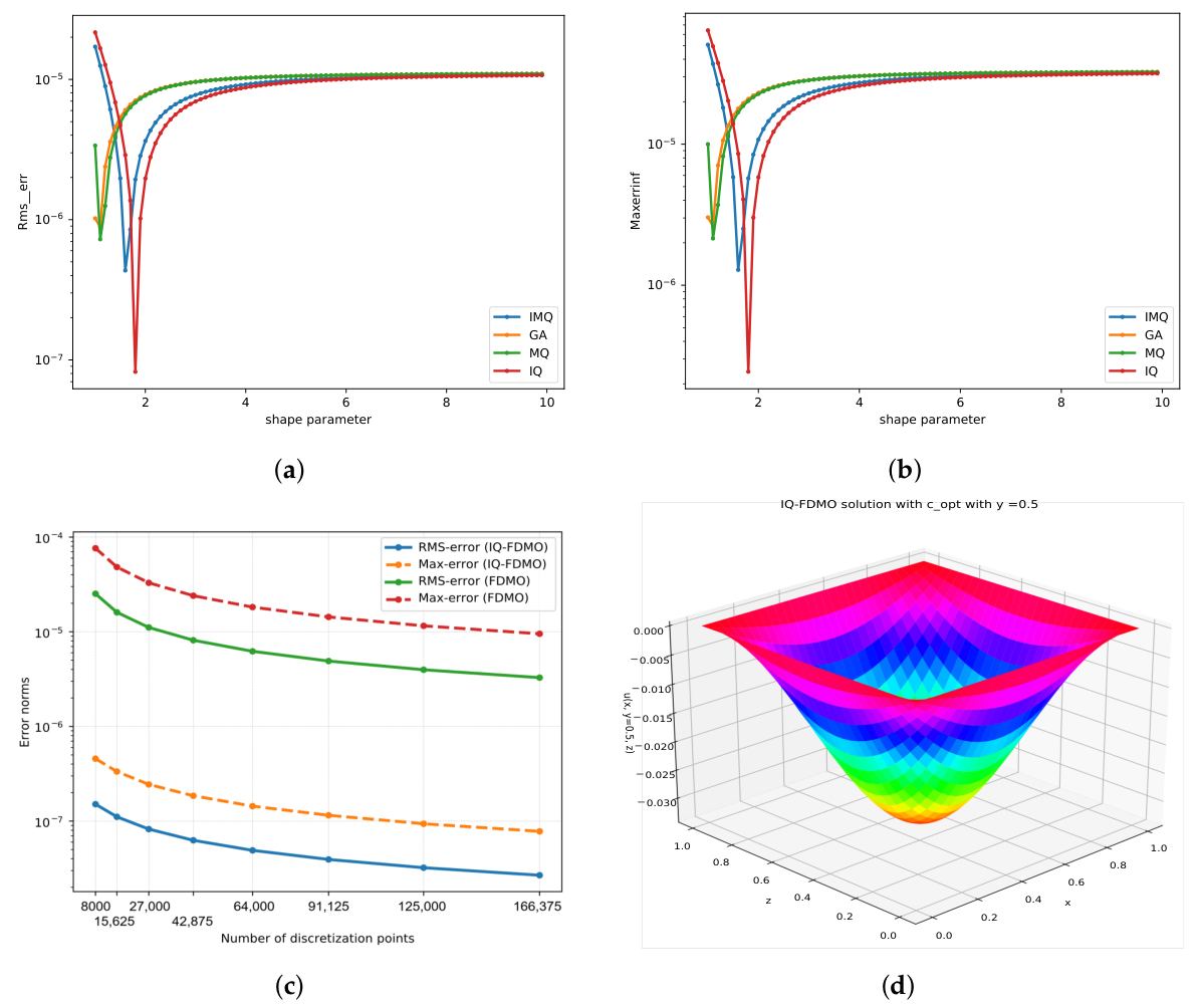
As illustrated in Figure 1a,b, the RMS and maximum error norms provide a clear assessment of the RBF-FDMO method’s performance in identifying the optimal shape parameter discussed in Section 3. Both error metrics reach their minimum at approximately $c_{\mathrm{opt}}\approx 1.8$, suggesting a balance between approximation accuracy and numerical stability.

Figure 1. RBF-FDMO solution and error norms of the 3-D benchmark problem. (a) RMS error norm of the RBF-FDMO solution vs. shape parameter. (b) Max error norm of the RBF-FDMO solution vs. shape parameter. (c) Comparison of error norms between the IQ-FDMO and FDMO solutions. (d) Three-dimensional IQ-FDMO solution at y = 0.5.

Figure 1a,b also provide a comparative assessment of the numerical performance of the GA, MQ, IQ, and IMQ radial basis functions. It can be observed that all RBFs are sensitive to the choice of the shape parameter, with each curve exhibiting a distinct minimum. Among them, the IQ function consistently yields lower RMS and maximum errors within the tested range, indicating a more favorable balance between accuracy and numerical stability. Based on this observation, the IQ function is adopted in the subsequent grounding-system simulations.

To enhance the robustness of these findings, further studies could include a finer sweep of c around $c_{\mathrm{opt}}$, examination of mesh sensitivity, or the use of automatic parameter-selection strategies such as leave-one-out cross-validation or condition-number-based optimization, thereby providing a more general framework for selecting shape parameters in practical RBF-FDMO applications.

Figure 1c presents a comparison of two error norms for the RBF-FDMO and FDMO methods as the discretization level N increases. The results demonstrate that the proposed approach markedly enhances accuracy, with the RMS error decreasing from ${10}^{-5}$ to ${10}^{-7}$ and the maximum error from ${10}^{-4}$ to ${10}^{-6}$, corresponding to an improvement of more than two orders of magnitude over the 3-D FDMO method [17]. Particularly, the RBF-FDMO method achieves comparable accuracy with a significantly smaller number of points, indicating favorable computational economy in the benchmark problem. Unlike the 3-D FDMO method [17], which demands thousands of points to reach similar levels of accuracy, the RBF-FDMO method manages to maintain high precision with far fewer points, making it a more computationally economical approach. This reduction in the number of required points, combined with its consistent stability, makes the RBF-FDMO method a powerful tool for efficiently solving 3-D science and engineering problems.

Finally, Figure 1d illustrates the 3-D solution obtained using the IQ-FDMO method with the optimal shape parameter, further confirming the accuracy and effectiveness of the proposed method in handling complex systems.

4.2. RBF-FDMO Approach for GS Analysis

The electric field produced by a GS embedded in homogeneous soil can be represented by the scalar potential $\phi$, which satisfies Laplace’s equation under the corresponding boundary conditions. Specifically, within the 3-D domain $\Omega$, the Laplace equation governs the potential, whereas the two-dimensional boundary $\Gamma$ is subject to particular constraints, such as those on the earth’s surface and at infinity. The governing equations can be formulated as follows:

• In the computational domain $\Omega$:

  $$\nabla ·\left(\right[\sigma ]\nabla \phi )=0$$

  (32)
• On the boundary $\Gamma$:

  $$\phi =0(r\to \infty ),{\displaystyle \frac{\partial \phi }{\partial n}}=0\left(\mathrm{in}\mathrm{earth}\mathrm{surface}\right).$$

  (33)

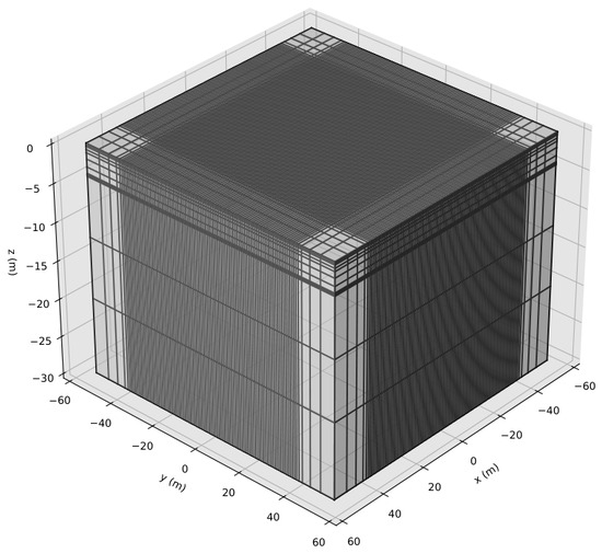
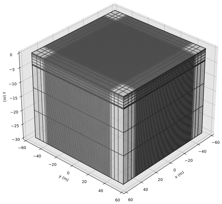
The IQ-FDMO solution of (32) allows the electric potential $\phi$ and the associated current density $\sigma$ to be computed with high accuracy at arbitrary locations $(x,y,z)$ on a non-uniform FD mesh within the computational domain, as depicted in Figure 2 of [17].

Figure 2. Model of non-uniform FD mesh [17].

In the numerical examples presented in this study, the soil is assumed to be homogeneous in order to focus on the formulation and validation of the proposed RBF-FDMO method under a well-defined modeling framework. This assumption is also consistent with benchmark configurations commonly used for methodological verification and comparison. The solution assumes that the GS is energized to a specified potential ${\phi }_{\Gamma }$, commonly referred to as the Ground Potential Rise (GPR), measured with respect to a remote earth reference. This formulation enables a detailed characterization of the electromagnetic behavior of the GS.

4.2.1. Case 1: Square-Shaped GS

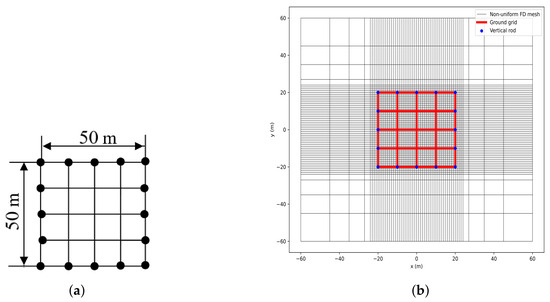
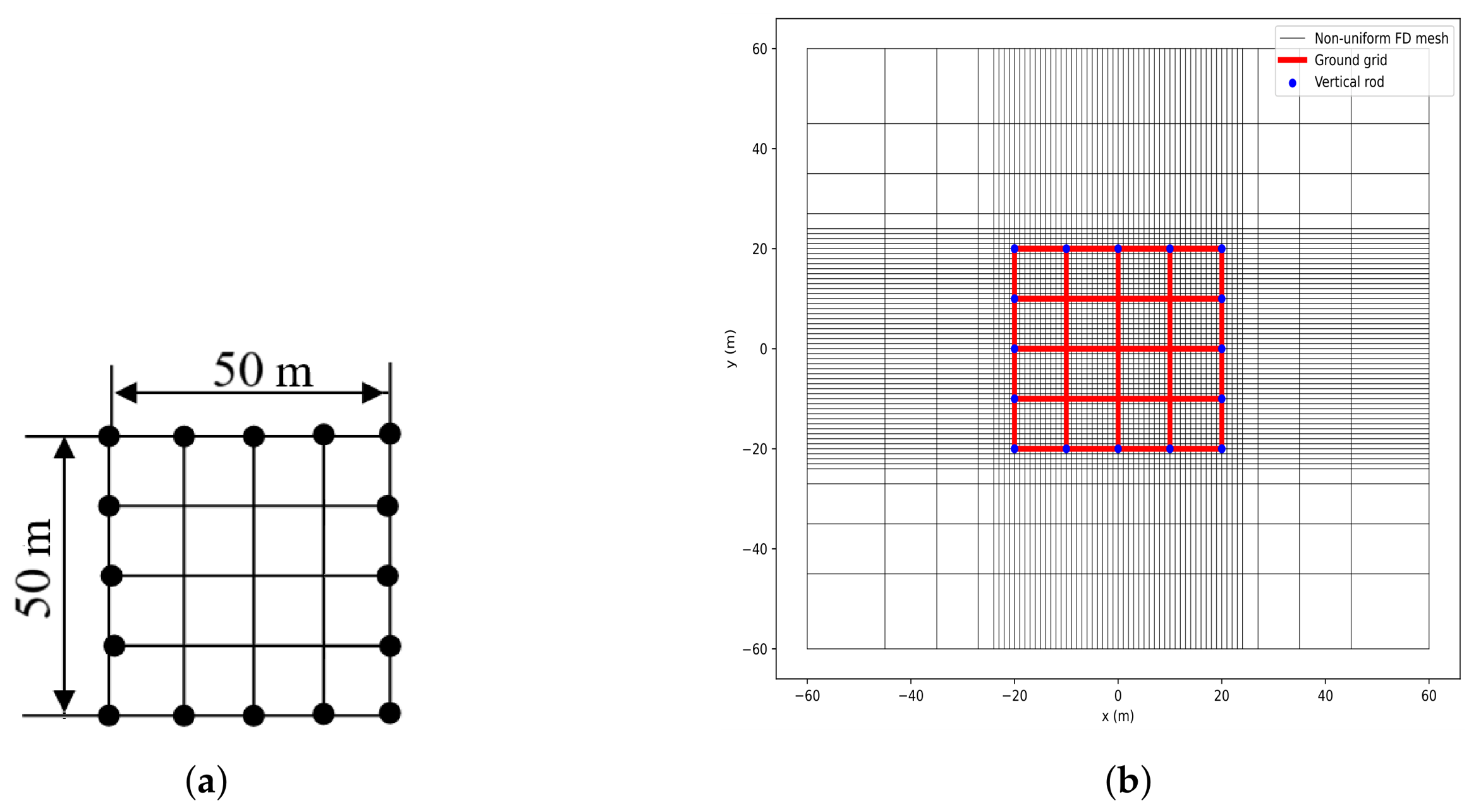
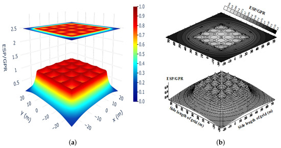
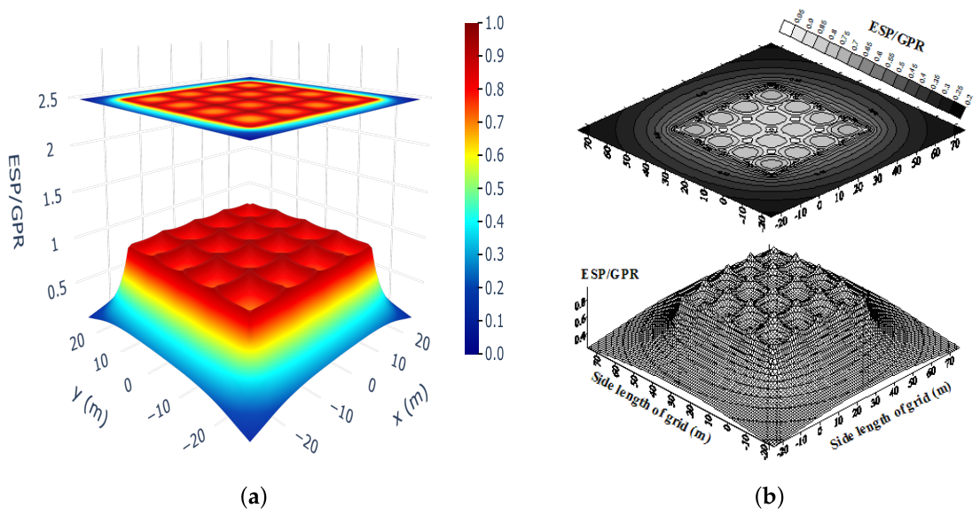
The R04P16 GS in [26] is selected as the first test case to evaluate the proposed method. The grid has dimensions of $50\mathrm{m}\times 50\mathrm{m}$ and consists of conductors spaced $12.5\mathrm{m}$ apart, forming a $4\times 4$ mesh configuration. This GS is buried at a depth of 0.5 m and includes vertical grounding rods of 2 m length and 5 mm radius placed along the perimeter, as illustrated in Figure 3a. The soil resistivity is assumed to be $\rho =2000\Omega ·\mathrm{m}$, and the GPR is set to 1 V. Using a shape parameter $c=1.3$ and applying the IQ-FDMO method with non-uniform FD mesh (shown in Figure 3b), the simulation results are presented in Figure 4a and summarized in Table 2.

Figure 3. The square-shaped GS: (a) model in [26]; (b) model using a nonuniform FD mesh.

Figure 4. Potential distributions of the square-shaped GS: (a) solution of the proposed IQ-FDMO method; (b) solution of the BEM in [26].

Table 2. Comparison of earth resistance, GPR, touch voltage, and step voltage for a fault current of $I_G=1\mathrm{kA}$.

Method	${\mathit{R}}_{\mathit{g}}$ ($\Omega$)	GPR (kV)	${\mathit{V}}_{\mathit{t},\mathbf{max}}$ (%)	${\mathit{V}}_{\mathit{s},\mathbf{max}}$ (%)
IQ-FDMO	20.1	20.1	28.2	10.0
BEM [26]	19.9	19.9	28.0	16.0
IEEE Std 80™ [1]	21.3	21.3	24.9	11.7

where $V_{t,\max }$ and $V_{s,\max }$ are the maximum touch and step voltages, respectively, expressed as percentages of GPR.

The performance of the IQ-FDMO method is evaluated against the BEM [26] and IEEE Std. 80™ [1] for the GS with a fault current of $I_G=1\mathrm{kA}$, considering parameters such as earth resistance ($R_g$), GPR, maximum touch voltage ($V_{t,\max }$), and maximum step voltage ($V_{s,\max }$). The IQ-FDMO achieves $R_g=20.1\Omega$ and GPR = 20.1 kV, closely matching the BEM result of $19.9\Omega$, and offers a 5.6% reduction in earth resistance compared to IEEE Std. 80™ ($21.3\Omega$). For touch voltage, IQ-FDMO yields $V_{t,\max }=28.2\%$, showing excellent agreement with BEM (28%) and exceeding IEEE Std. 80 (24.9%), indicating a conservative yet accurate safety assessment comparable to BEM. Notably, IQ-FDMO produces the lowest step voltage at $V_{s,\max }=10\%$, representing a 37.5% decrease from BEM (16%) and a 14.5% decrease from IEEE Std. 80™ (11.7%), thereby significantly enhancing safety by reducing step voltage hazards. These results demonstrate that IQ-FDMO combines high accuracy—closely matching BEM—with superior step voltage mitigation, making it a highly effective method for grounding system design.

4.2.2. Case 2: Rectangular-Shaped GS

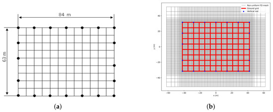
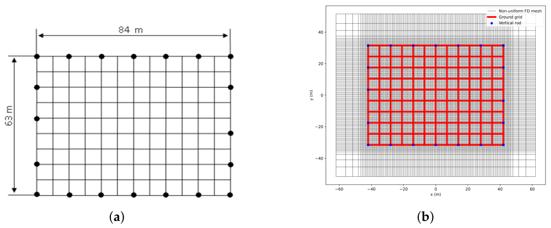
The GS under study has a rectangular layout measuring 63 m by 84 m [1]. The conductors are arranged with a spacing of 7 m, forming a mesh of 10 by 10 interconnected segments. The grid is buried at a depth of 0.8 m, with vertical rods (3 m long and 10 mm in diameter) placed along its boundary, as shown in Figure 5a. The soil resistivity is $\rho =400\Omega ·\mathrm{m}$ and the maximum grid current is $I_G=1.908\mathrm{kA}$. The configuration is discretized using a non-uniform FD mesh for the IQ–FDMO simulation, as illustrated in Figure 5b.

Figure 5. The rectangular-shaped GS (a) in IEEE Std 80™ [1]; (b) in non-uniform FD mesh.

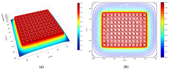
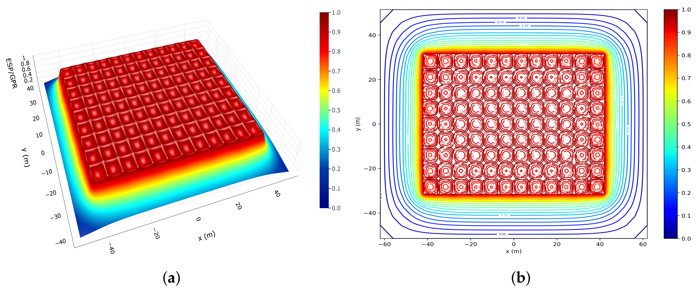
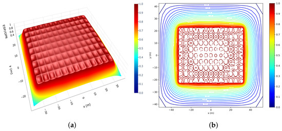
Figure 6 shows the potential distribution and corresponding equipotential contours over the grid, highlighting the electric field behavior within the GS. Figure 7 compares the ESP results from the IQ–FDMO method with those from the FE model.

Figure 6. The IQ-FDMO solutions of the rectangular-shaped GS: (a) 3-D potentials distribution; (b) equipotential lines on the ground surface.

Figure 7. Comparison of the IQ-FDMO and FE solutions of the potential distributions in the rectangular-shaped GS: (a) $x=0$; (b) $y=3$.

The comparison results Table 3 show that the maximum and minimum potentials computed by both methods are in close agreement. Specifically, the results indicate that the maximum potential computed using the IQ–FDMO scheme is ${\phi }_{\max }=0.994$ pu, which is marginally higher than the value obtained with the FEM approach ($0.993$ pu). In contrast, the minimum potential estimated by IQ–FDMO reaches ${\phi }_{\min }=0.845$ pu, slightly lower than the corresponding FEM result ($0.866$ pu). In addition, the peak potential variation predicted by IQ–FDMO, $\Delta {\phi }_{\max }=0.149$ pu, exceeds the FEM value of $0.127$ pu. These small deviations arise from the inherent differences in mesh construction and numerical discretization adopted by the two methods. The close agreement between the two sets of results confirms the accuracy of the proposed method. Furthermore, IQ-FDMO offers several advantages over FEM, including operator-based implementation on non-uniform finite-difference grids, greater flexibility in handling irregular geometries, and reduced computational complexity during pre-processing. These features make RBF-FDMO a promising alternative for efficient and accurate analysis of grounding systems in complex environments.

Table 3. Comparison of electric potential calculated using IQ-FDMO and FEM for rectangular-shaped grounding system (GS).

Method	${\mathit{\phi }}_{\mathbf{max}}$ (pu)	${\mathit{\phi }}_{\mathbf{min}}$ (pu)	$\Delta {\mathit{\phi }}_{\mathbf{max}}$ (pu)
IQ-FDMO	0.994	0.845	0.149
FEM	0.993	0.866	0.127

where ${\phi }_{\max }$, ${\phi }_{\min }$, and $\Delta {\phi }_{\max }$ correspond to the maximum and minimum ground surface potentials and the maximum potential difference, respectively.

Furthermore, as shown in Table 4, the IQ-FDMO method achieves an earth resistance of $R_g=2.66\Omega$, which is 1.14% higher than that of IEEE Std. 80™ ($2.63\Omega$). The GPR value is also slightly elevated at 5.03 kV, marking a 0.2% increase compared to 5.02 kV. Regarding touch voltage, IQ-FDMO yields $V_{t,\max }=14.9\%$, which is 0.68% higher than IEEE Std. 80™ (14.8%). Most notably, IQ-FDMO significantly reduces the maximum step voltage to 6.0%, representing a 22.7% decrease compared to IEEE Std. 80™ (7.76%). These results underscore the accuracy and reliability of the proposed method in evaluating GS safety, reinforcing its potential as a robust and efficient alternative to conventional numerical techniques.

Table 4. Computed safety parameters of the rectangular GS using IQ–FDMO compared with IEEE Std. 80™.

Method	${\mathit{R}}_{\mathit{g}}$ ($\Omega$)	GPR (kV)	${\mathit{V}}_{\mathit{t},\mathbf{max}}$ (%)	${\mathit{V}}_{\mathit{s},\mathbf{max}}$ (%)
IQ-FDMO	2.66	5.03	14.9	6.0
IEEE Std 80™ [1]	2.63	5.02	14.8	7.76

4.2.3. Case 3: L-Shaped GS

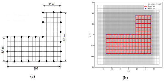
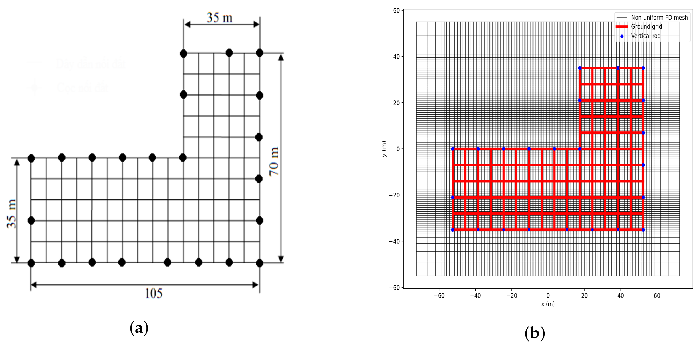
To investigate a different grounding layout, an L-shaped GS is examined. The grid occupies a main area of 105 m by 70 m and includes an additional 35 m by 35 m section extending from one corner, consistent with the configuration reported in [1]. The conductors are spaced 7 m apart, yielding 100 mesh cells. The grid is buried at a depth of 0.8 m, with vertical rods (3 m long and 10 mm in diameter) installed along the boundary at intervals of two to three mesh cells, as shown in Figure 8a. The soil resistivity is $\rho =400\Omega ·\mathrm{m}$ and the maximum grid current is $I_G=1.908\mathrm{kA}$. The computational domain covers an area of 145 m × 110 m with a depth of 30 m. The L-shaped grounding system is discretized using a non-uniform FD mesh, similar to the rectangular case, as illustrated in Figure 8b.

Figure 8. The L-shaped GS with vertical rods along its perimeter: (a) in IEEE Std 80™ [1]; (b) in non-uniform FD mesh.

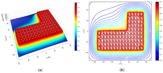
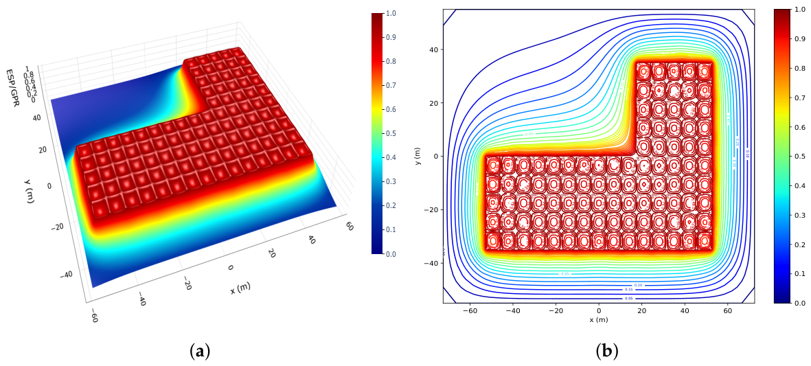
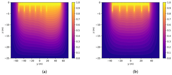
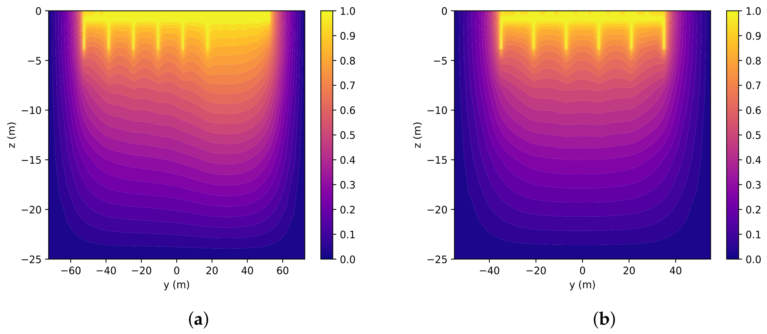
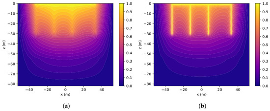
The simulation results of the potential distribution for the L-shaped GS, shown in both 3-D and 2-D views in Figure 9 and Figure 10, respectively, illustrate the applicability and versatility of the proposed RBF-FDMO method in accurately modeling the GS with arbitrary geometries.

Figure 9. IQ–FDMO results for the L-shaped GS: (a) 3D potential distribution; (b) ground surface equipotential contours.

Figure 10. Soil equipotential contours of the L-shaped GS: (a) center (x-axis); (b) boundary region.

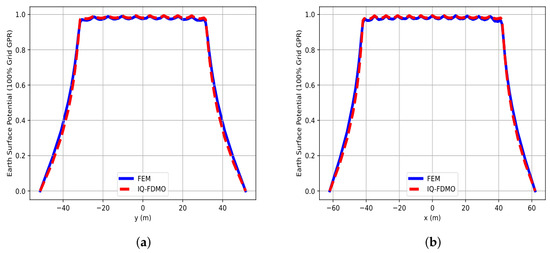
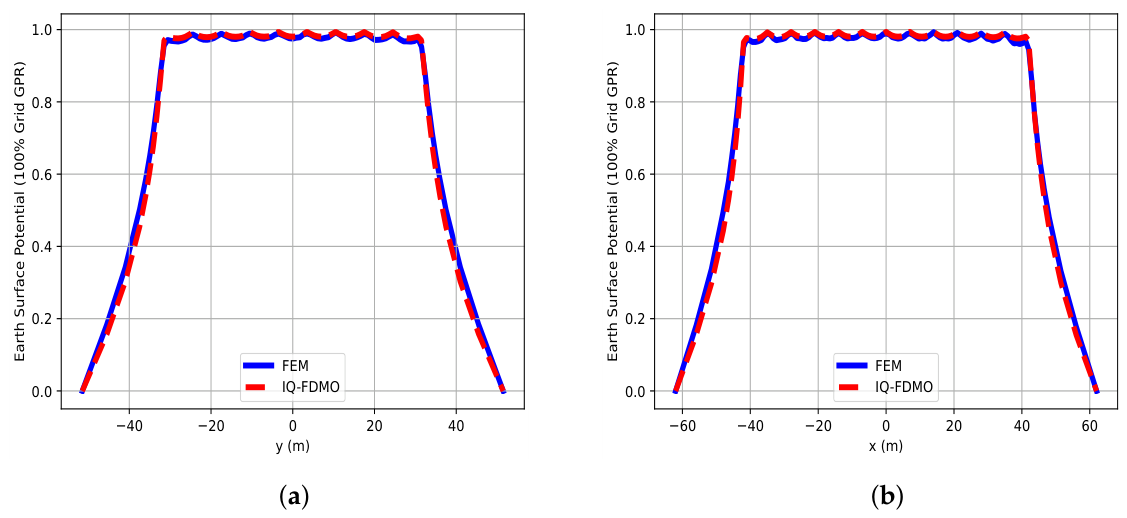
Figure 11 and Table 5 show a comparison of potential distributions obtained using IQ–FDMO and the FEM for the L-shaped grounding system. Both methods produce nearly identical maximum and minimum potentials, with IQ–FDMO yielding a slightly higher peak and a slightly lower minimum. The difference in maximum potential variation is small, indicating that IQ–FDMO accurately reproduces the spatial potential distribution. These results confirm that IQ–FDMO is a reliable alternative to the FEM for GSs with irregular geometries.

Figure 11. Comparison of the IQ-FDMO and FE solutions of the potential distributions in the L-shaped GS: (a) $x=-18$ m; (b) $y=18$ m.

Table 5. Potential distribution in the L-shaped grounding system: IQ–FDMO versus FEM.

Method	${\mathit{\phi }}_{\mathbf{max}}$ (pu)	${\mathit{\phi }}_{\mathbf{min}}$ (pu)	$\Delta {\mathit{\phi }}_{\mathbf{max}}$ (pu)
IQ-FDMO	0.995	0.846	0.149
FEM	0.993	0.864	0.129

Table 6 compares the performance of the IQ-FDMO method with the IEEE Std 80™ guidelines in evaluating the touch and step voltages for the L-shaped grounding system (GS). Both approaches yield identical values for ground resistance ($R_g=2.74\Omega$) and ground potential rise (GPR = 5.23 kV), indicating consistency in their estimation of fundamental grounding parameters. However, slight differences are observed in the predicted safety voltages. Specifically, the IQ-FDMO method estimates a maximum touch voltage ($V_{t,\max }$) of 14.9% and a maximum step voltage ($V_{s,\max }$) of 6.0%, which are marginally lower than the corresponding IEEE Std 80™ values of 15.4% and 8.1%, respectively. These deviations suggest that IQ-FDMO may offer a more refined and potentially conservative evaluation of voltage profiles, supporting its effectiveness and reliability for the safety assessment of GS with arbitrary geometries.

Table 6. Evaluation of key safety parameters for the L-shaped grounding system using IQ–FDMO in comparison with IEEE Std. 80™.

Approach	${\mathit{R}}_{\mathit{g}}$ ($\Omega$)	GPR (kV)	${\mathit{V}}_{\mathit{t},\mathbf{max}}$ (%)	${\mathit{V}}_{\mathit{s},\mathbf{max}}$ (%)
IQ-FDMO	2.74	5.23	14.9	6.0
IEEE Std 80™ [1]	2.74	5.23	15.4	8.1

4.2.4. Case 4: Practical GS in Vietnam

This section analyzes the grounding system of the 110 kV–63 MVA Da Mi floating solar substation, part of Vietnam’s renewable energy expansion program. The site is located on the Da Mi hydropower reservoir in Ham Thuan Bac District, Binh Thuan Province. The integration of floating PV technology with an existing hydropower plant offers an efficient and sustainable energy solution.

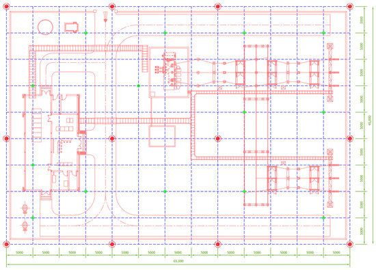
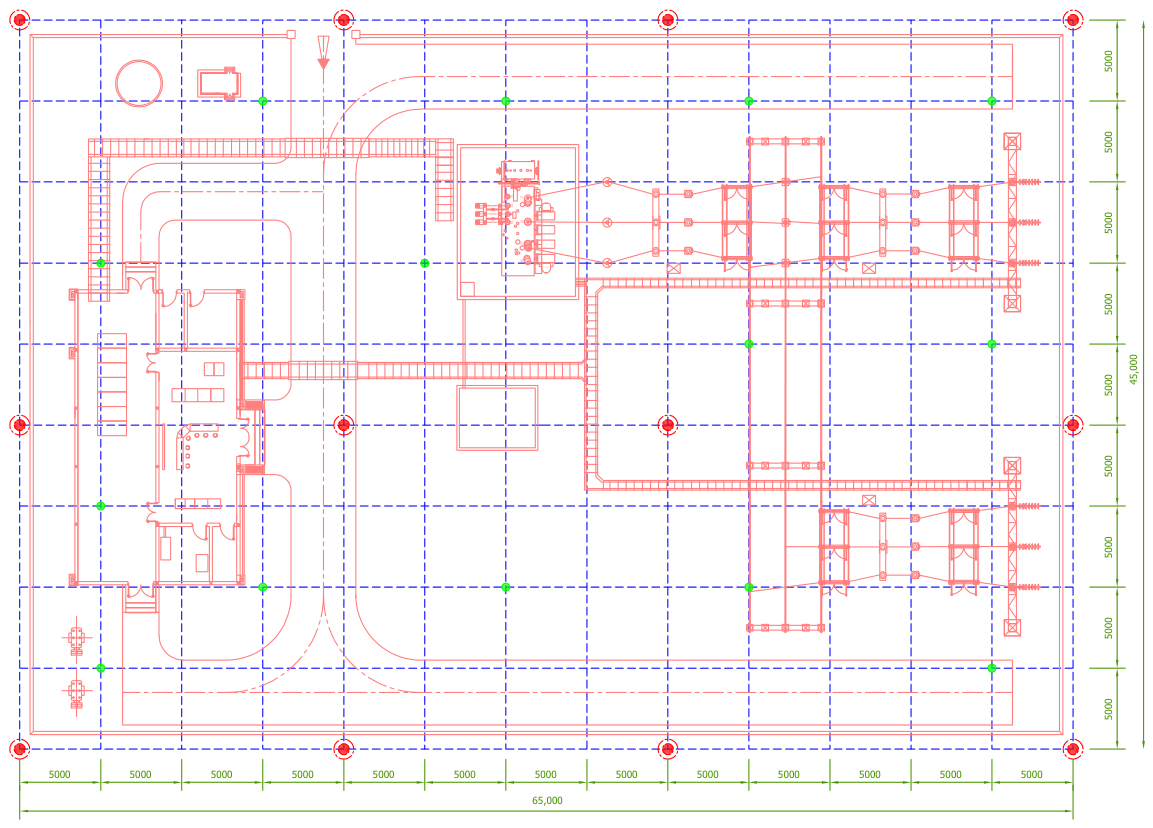
Figure 12 depicts the configuration of the grounding system and the corresponding equipment layout for the solar substation, which spans an area of $65\times 45$ m. The grounding grid is constructed from galvanized steel conductors with a diameter of 14 mm and is supplemented by vertical rods (green dots) of identical diameter and 3 m length. Furthermore, GEM wells (red dots) are included in the design, consisting of steel electrodes with a diameter of 120 mm installed to a depth of 30 m. All grounding components are buried at a consistent depth of 0.8 m to maintain effective operation and structural longevity.

Figure 12. Layout of the GS and equipment for the solar power substation in Vietnam.

The GS is characterized by key parameters under fault conditions. For a phase-to-ground fault, a current of $I_g=8.42\mathrm{kA}$ with a duration of 0.5 s is applied to evaluate step and touch voltage limits. The soil resistivity is $\rho =300\Omega ·\mathrm{m}$, which influences the potential distribution. The total grounding resistance, including the substation contribution, is $R_{GS}=0.49\Omega$, ensuring effective fault current dissipation and compliance with safety requirements.

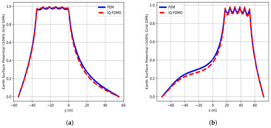
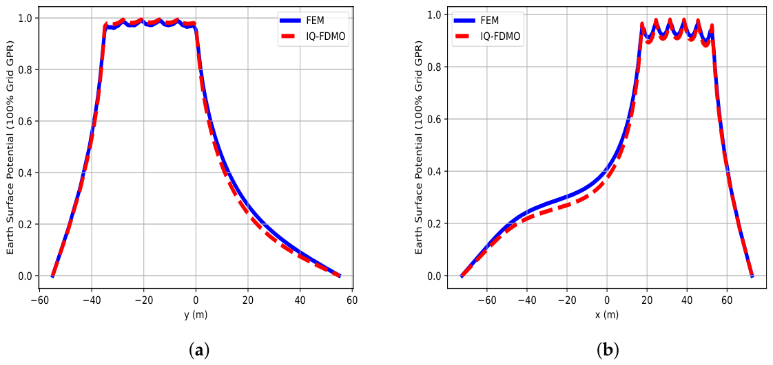
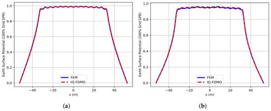
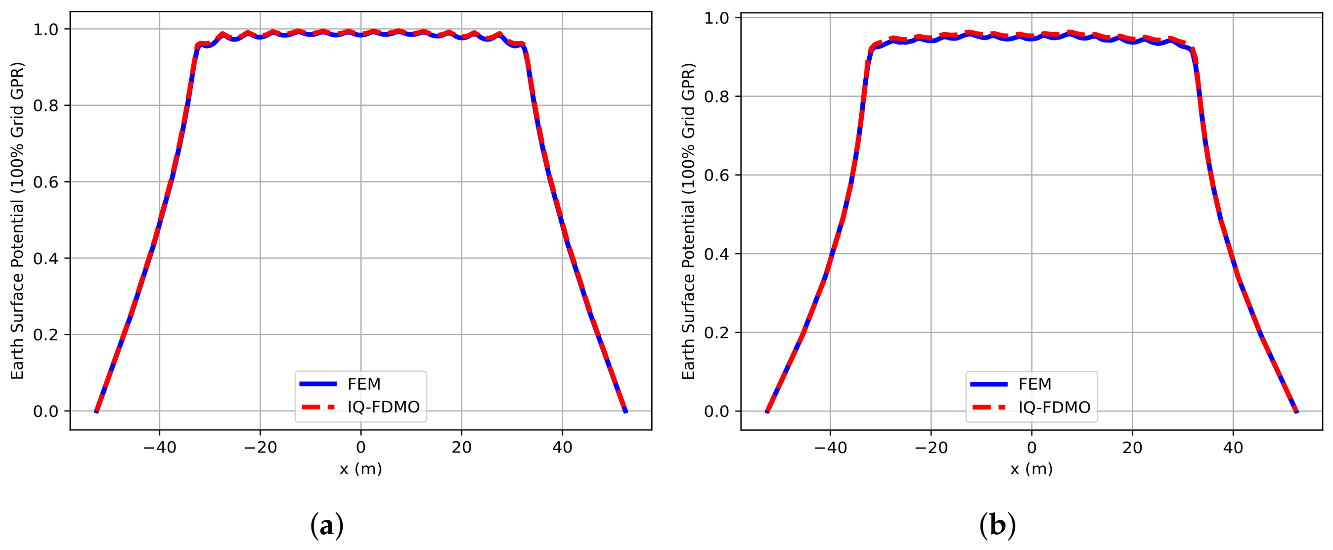
The IQ-FDMO approach was employed to evaluate the real-world GS in Vietnam, producing the potential distribution and equipotential patterns shown in Figure 13 and Figure 14. A comparison of the Earth Surface Potential (ESP) obtained from the IQ-FDMO and FE simulations is presented in Figure 15a,b, with the corresponding numerical summary listed in Table 7. The results reveal that both techniques yield closely matching potential profiles across the grounding area. While the two methods generally agree well, IQ-FDMO tends to predict marginally higher variations in potential, providing a slightly more conservative perspective that can be advantageous for ensuring safety compliance. In addition, the reduced mathematical complexity and lower computational burden of IQ-FDMO make it an efficient tool for fast yet reliable assessments. These advantages highlight IQ-FDMO as a practical and robust alternative to traditional FE-based analysis.

Figure 13. IQ–FDMO results for the practical GS: (a) 3D potential distribution; (b) ground surface equipotential contours.

Figure 14. Equipotential contours in soil for the practical GS: (a) center (x-axis); (b) boundary region.

Figure 15. Potential distributions in the practical GS: IQ–FDMO versus FEM for (a) $x=y$ and (b) $y=0$.

Table 7. Potential distribution in the practical GS: IQ–FDMO versus FEM.

Method	${\mathit{\phi }}_{\mathbf{max}}$ (pu)	${\mathit{\phi }}_{\mathbf{min}}$ (pu)	$\Delta {\mathit{\phi }}_{\mathbf{max}}$ (pu)
IQ-FDMO	0.997	0.897	0.100
FEM	0.997	0.878	0.119

As indicated in Table 8, the computed grounding resistance of 0.5 $\Omega$ agrees very well with the on-site measurement of 0.49 $\Omega$, presenting a difference of only 0.01 $\Omega$. Considering a human body weight of 70 kg, the maximum touch voltage normalized to the GPR, $V_{t,\max }=10.1\%$, remains far below the IEEE Std 80™ limit of 25.1%, yielding a safety margin of nearly 59.8%. Likewise, the maximum step voltage per GPR, $V_{s,\max }=3.03\%$, is substantially lower than the permissible 12.98% threshold for the same body weight, corresponding to an approximate margin of 76.7%. The IEEE Std 80™ criteria used for these evaluations are derived according to the formulas summarized in Appendix B. These results demonstrate not only the strong performance and reliability of the grounding system but also highlight the precision and practical applicability of the IQ-FDMO approach when analyzing real-world substation installations. Overall, the system fully satisfies safety standards, requiring no additional corrective measures and ensuring secure operation under high-voltage fault conditions.

Table 8. Safety parameters of the practical GS obtained with IQ–FDMO.

${\mathit{R}}_{\mathit{g}}$ ($\Omega$)	GPR (kV)	${\mathit{V}}_{\mathit{t},\mathbf{max}}$ (%)	${\mathit{V}}_{\mathit{s},\mathbf{max}}$ (%)
0.5	2.5	10.1	3.03

5. Remarks and Conclusions

Here, we can remark some main points as follows:

• Mathematical Formulation: Compared with numerical techniques such as the FEM, BEM, and MoM, the FDM stands out for its conceptual and computational simplicity. Its mathematical structure is considerably more direct, which simplifies coding, algorithmic management, and overall implementation. When combined with the RBF–FDMO framework, three-dimensional problems can be formulated efficiently by constructing the system through successive Kronecker products of the corresponding one-dimensional operators, as described in Section 2.2. This strategy is particularly effective for large-scale domains, intricate geometries, and a wide range of boundary condition types, making it a robust choice for practical engineering applications.
• Accuracy: When RBF approximations are employed as substitutes for the classical Taylor-series-based FD approximations, the RBF-FDMO approach demonstrates markedly improved accuracy compared to traditional numerical methods in the small value range of the shape parameter. In particular, when the RBF-FDMO approach is combined with an optimal shape parameter selection algorithm, as presented in [20], results such as those shown in Figure 1a,b can be obtained.
• Cost-efficient: As illustrated in Figure 1c, the RBF–FDMO approach attains an accuracy comparable to, or in some cases better than, the FDMO solution while using only a few thousand nodes in the discretized domain. In contrast, the FDMO method requires several hundred thousand points to reach a similar error level. This demonstrates that RBF-FDMO can substantially alleviate computational demands, making it well suited for large-scale or geometrically intricate problems where extremely high precision is not essential.
• Applicability: The RBF–FDMO framework can accommodate various GS configurations, including square, rectangular, L-shaped, and practical substation layouts. With its low computational complexity and simple implementation, it serves as an efficient tool for GS design and optimization in high-voltage substations. It also enables the evaluation of key safety parameters, such as grounding resistance and step and touch voltage limits, in accordance with IEEE, IEC, and national standards, as described in Section 4.

This paper presents the development of the RBF–FDMO method, which extends the previously proposed FDMO formulation [17,21] to fully three-dimensional problems through the use of Kronecker products of one-dimensional differential operators. This extension represents a significant methodological advancement, as it enables the efficient construction of multi-dimensional finite-difference operators without the need for complex mesh generation or domain discretization typically required in FEM-based solvers. By integrating RBFs into the FDMO framework, the proposed approach significantly enhances the accuracy, smoothness, and numerical stability of derivative approximations, thus achieving a better trade-off between precision and computational cost.

It should be noted that the present work is conducted under idealized conditions, including homogeneous soil assumptions and standardized grounding configurations. In addition, the computational efficiency demonstrated here is reflected mainly in the simplicity of the operator-based formulation and in the ability of the proposed method to achieve high accuracy with relatively fewer discretization points in the benchmark problem, rather than through a full runtime- and memory-based benchmark. A more comprehensive analysis of convergence behavior, computational performance, and extensions to more complex soil models and grounding configurations will be considered in future work.

The novelty of this study lies in formulating a 3-D RBF-enhanced finite-difference operator scheme on uniform and non-uniform nodal grids that inherits the simplicity of the conventional FDM while leveraging the flexibility of RBF interpolation to handle irregular node distributions and complex geometries. Unlike traditional numerical methods such as the FEM, BEM, or MoM, which rely heavily on meshing or the evaluation of integral kernels, the RBF–FDMO constructs purely algebraic operators that can be easily implemented and adapted to diverse GS configurations and heterogeneous soil conditions. The proposed method was validated using a well-established 3-D benchmark problem, where the RBF–FDMO solution demonstrated superior accuracy compared with the corresponding FDMO results. Following this validation, the method was successfully applied to simulate the potential distribution of grounding systems with various geometries, including a real-world 110-kV substation in Vietnam. The simulation results exhibited excellent agreement with those obtained from conventional numerical methods such as the FEM and BEM, while having competitive computational efficiency and providing a simpler numerical formulation.

Overall, this work contributes to the field by introducing a novel 3-D RBF–FDMO formulation that unifies the advantages of the FDM, RBF interpolation, and operator-based construction via Kronecker products. The method combines mathematical simplicity, high accuracy, and computational efficiency, offering a new numerical framework that bridges the gap between traditional mesh-based solvers and emerging meshless techniques. With its robustness and flexibility, the RBF–FDMO method shows strong potential for practical grounding system analysis, especially in early-stage design and optimization tasks in high-voltage substation projects, where rapid assessment of multiple GS configurations is essential. Future work will focus on extending this framework to transient and frequency-dependent analyses and on integrating it into commercial grounding design software and power utility workflows.

Appendix A.1. Central Approximations

Substituting (A1) into (5) and (A2) into (6), evaluated at $x_{i-1}$, $x_i$, and $x_{i+1}$, with $\Delta x_1=x_i-x_{i-1}$, $\Delta x_2=x_i-x_{i+1}$, and $\Delta x_3=x_{i+1}-x_{i-1}$, yields two linear systems, which can be written in matrix form.

It is important to note that the same procedure can be applied to determine the unknown weight coefficients for other types of RBFs, such as the MQ, IQ, and IMQ functions. Solving these systems provides a general framework for calculating the coefficients used in finite difference approximations of derivatives, thereby ensuring that the method remains flexible and applicable to a wide range of RBFs and problem types.

$$\begin{array}{cc}\hfill \left[\begin{array}{c}{\displaystyle \frac{-2\Delta x_1}{c^2}}{e}^{-{(\Delta x_1)}^2/c^2}\\ 0\\ {\displaystyle \frac{-2\Delta x_2}{c^2}}{e}^{-{(\Delta x_2)}^2/c^2}\end{array}\right]& =\left[\begin{array}{ccc}1& e^{-{(\Delta x_1)}^2/c^2}& e^{-{(\Delta x_3)}^2/c^2}\\ e^{-{(\Delta x_1)}^2/c^2}& 1& e^{-{(\Delta x_2)}^2/c^2}\\ e^{-{(\Delta x_3)}^2/c^2}& e^{-{(\Delta x_2)}^2/c^2}& 1\end{array}\right]\left[\begin{array}{c}{\alpha }_1^{GA}\\ {\alpha }_2^{GA}\\ {\alpha }_3^{GA}\end{array}\right]\hfill \end{array}$$

(A3)

$$\begin{array}{ccc}\hfill \left[\begin{array}{c}{\displaystyle \frac{2}{c^2}}\left({\displaystyle \frac{2{(\Delta x_1)}^2}{c^2}}-1\right)e^{-{(\Delta x_1)}^2/c^2}\\ {\displaystyle \frac{-2}{c^2}}\\ {\displaystyle \frac{2}{c^2}}\left({\displaystyle \frac{2{(\Delta x_2)}^2}{c^2}}-1\right)e^{-{(\Delta x_2)}^2/c^2}\end{array}\right]& =\left[\begin{array}{ccc}1& e^{-{(\Delta x_1)}^2/c^2}& e^{-{(\Delta x_3)}^2/c^2}\\ e^{-{(\Delta x_1)}^2/c^2}& 1& e^{-{(\Delta x_2)}^2/c^2}\\ e^{-{(\Delta x_3)}^2/c^2}& e^{-{(\Delta x_2)}^2/c^2}& 1\end{array}\right]\hfill & \hfill \left[\begin{array}{c}{\beta }_1^{GA}\\ {\beta }_2^{GA}\\ {\beta }_3^{GA}\end{array}\right]\end{array}$$

(A4)

We can reformulate (A3) and (A4) as follows:

$${\mathbf{A}}_{GA}={\Psi }_{GA}{\mathsf{\alpha }}^{GA},$$

(A5)

$${\mathbf{B}}_{GA}={\Psi }_{GA}{\mathsf{\beta }}^{GA}.$$

(A6)

The weighting coefficients appearing in (A5) and (A6) are obtained by solving the associated linear algebraic systems. These systems arise by inserting the chosen Radial Basis Functions (RBFs) into the finite-difference stencil and enforcing the required derivative conditions at the selected nodes. After the system is formulated, the unknown coefficients can be computed using common numerical procedures, for example direct matrix factorization or iterative solution schemes. This procedure yields coefficients that are tailored to the local node distribution, thereby improving the accuracy of the derivative approximation. In addition, the same construction applies to different classes of RBFs, making the approach broadly applicable to the numerical solution of partial differential equations across various geometries and discretizations.

$${\mathsf{\alpha }}^{GA}={\Psi }_{GA}^{-1}{\mathbf{A}}_{GA},$$

(A7)

$${\mathsf{\beta }}^{GA}={\Psi }_{GA}^{-1}{\mathbf{B}}_{GA}.$$

(A8)

Appendix A.2. Forward and Backward Approximations

Following the same procedure as in the central-difference formulation, the forward-difference case is constructed by evaluating the Gaussian (GA) RBF representation at the nodes $x_i$, $x_{i+1}$, and $x_{i+2}$. Let $\Delta x_1=x_i-x_{i+1}$, $\Delta x_2=x_i-x_{i+2}$, and $\Delta x_3=x_{i+1}-x_{i+2}$. Based on this configuration, two linear systems are obtained using forward finite-difference approximations at the selected nodes, which can be written in matrix form as shown below.

The resulting formulation provides a consistent framework for embedding GA RBFs into the finite-difference scheme, allowing efficient evaluation of spatial derivatives. Owing to the flexibility of Gaussian RBFs, the approach can be extended straightforwardly to more complex geometries and boundary conditions, thereby offering a robust numerical tool for solving partial differential equations.

$$\begin{array}{ccc}\hfill \left[\begin{array}{c}0\\ {\displaystyle \frac{-2(\Delta x_1)}{c^2}}{e}^{-{(\Delta x_1)}^2/c^2}\\ {\displaystyle \frac{-2(\Delta x_2)}{c^2}}{e}^{-{(\Delta x_2)}^2/c^2}\end{array}\right]& =\left[\begin{array}{ccc}1& e^{-{(\Delta x_1)}^2/c^2}& e^{-{(\Delta x_2)}^2/c^2}\\ e^{-{(\Delta x_1)}^2/c^2}& 1& e^{-{(\Delta x_3)}^2/c^2}\\ e^{-{(\Delta x_2)}^2/c^2}& e^{-{(\Delta x_3)}^2/c^2}& 1\end{array}\right]\hfill & \hfill \left[\begin{array}{c}{\alpha }_{1F}^{GA}\\ {\alpha }_{2F}^{GA}\\ {\alpha }_{3F}^{GA}\end{array}\right].\end{array}$$

(A9)

$$\begin{array}{ccc}\hfill \left[\begin{array}{c}{\displaystyle \frac{-2}{c^2}}\\ {\displaystyle \frac{2}{c^2}}\left({\displaystyle \frac{2{(\Delta x_1)}^2}{c^2}}-1\right)e^{-{(\Delta x_1)}^2/c^2}\\ {\displaystyle \frac{2}{c^2}}\left({\displaystyle \frac{2{(\Delta x_2)}^2}{c^2}}-1\right)e^{-{(\Delta x_2)}^2/c^2}\end{array}\right]& =\left[\begin{array}{ccc}1& e^{-{(\Delta x_1)}^2/c^2}& e^{-{(\Delta x_2)}^2/c^2}\\ e^{-{(\Delta x_1)}^2/c^2}& 1& e^{-{(\Delta x_3)}^2/c^2}\\ e^{-{(\Delta x_2)}^2/c^2}& e^{-{(\Delta x_3)}^2/c^2}& 1\end{array}\right]\hfill & \hfill \left[\begin{array}{c}{\beta }_{1F}^{GA}\\ {\beta }_{2F}^{GA}\\ {\beta }_{3F}^{GA}\end{array}\right]\end{array}$$

(A10)

Similarly, by substituting the function with GA-RBFs at the points $x_i$, $x_{i-1}$, and $x_{i-2}$, and defining $\Delta x_1=x_i-x_{i-1}$, $\Delta x_2=x_i-x_{i-2}$, and $\Delta x_3=x_{i-1}-x_{i-2}$, we derive two systems of linear equations. These systems result from applying backward FD approximations at the selected nodes and can be represented in matrix form, as detailed below.

This formulation integrates GA-RBFs into backward difference schemes, offering an efficient and flexible framework for derivative approximation. The approach is well-suited for a wide range of boundary conditions and problem domains, particularly those involving complex geometries or non-uniform discretization.

$$\begin{array}{ccc}\hfill \left[\begin{array}{c}0\\ {\displaystyle \frac{-2(\Delta x_1)}{c^2}}{e}^{-{(\Delta x_1)}^2/c^2}\\ {\displaystyle \frac{-2(\Delta x_2)}{c^2}}{e}^{-{(\Delta x_2)}^2/c^2}\end{array}\right]& =\left[\begin{array}{ccc}1& e^{-{(\Delta x_1)}^2/c^2}& e^{-{(\Delta x_2)}^2/c^2}\\ e^{-{(\Delta x_1)}^2/c^2}& 1& e^{-{(\Delta x_3)}^2/c^2}\\ e^{-{(\Delta x_2)}^2/c^2}& e^{-{(\Delta x_3)}^2/c^2}& 1\end{array}\right]\hfill & \hfill \left[\begin{array}{c}{\alpha }_{1B}^{GA}\\ {\alpha }_{2B}^{GA}\\ {\alpha }_{3B}^{GA}\end{array}\right]\end{array}$$

(A11)

$$\begin{array}{ccc}\hfill \left[\begin{array}{c}{\displaystyle \frac{-2}{c^2}}\\ {\displaystyle \frac{2}{c^2}}\left({\displaystyle \frac{2{(\Delta x_1)}^2}{c^2}}-1\right)e^{-{(\Delta x_1)}^2/c^2}\\ {\displaystyle \frac{2}{c^2}}\left({\displaystyle \frac{2{(\Delta x_2)}^2}{c^2}}-1\right)e^{-{(\Delta x_2)}^2/c^2}\end{array}\right]& =\left[\begin{array}{ccc}1& e^{-{(\Delta x_1)}^2/c^2}& e^{-{(\Delta x_2)}^2/c^2}\\ e^{-{(\Delta x_1)}^2/c^2}& 1& e^{-{(\Delta x_3)}^2/c^2}\\ e^{-{(\Delta x_2)}^2/c^2}& e^{-{(\Delta x_3)}^2/c^2}& 1\end{array}\right]\hfill & \hfill \left[\begin{array}{c}{\beta }_{1B}^{GA}\\ {\beta }_{2B}^{GA}\\ {\beta }_{3B}^{GA}\end{array}\right]\end{array}$$

(A12)

Finally, (A9) and (A10), or alternatively (A11) and (A12), can be reformulated into the matrix forms of (A5) and (A6). The corresponding weight coefficients can then be computed using Equations (A7) and (A8).

Appendix B.1. Tolerable Touch Voltage and Step Voltage for Human

According to IEEE Std 80™ [1], and assuming a minimum predictable body weight of 70 kg, the maximum allowable touch voltage $V_{t,\mathrm{tolerance}}$ and step voltage $V_{s,\mathrm{tolerance}}$ can be calculated as follows:

$$\begin{array}{cc}\hfill V_{t,tolerance}& ={\displaystyle \frac{(1000+1.5C_s{\rho }_s)0.157}{\sqrt{t_s}}}\hfill \end{array}$$

(A13)

$$\begin{array}{cc}\hfill V_{s,tolerance}& ={\displaystyle \frac{(1000+6C_s{\rho }_s)0.157}{\sqrt{t_s}}}\hfill \end{array}$$

(A14)

where $C_s$ denotes the surface layer derating factor, ${\rho }_s$ represents the surface material resistivity $(\Omega ·\mathrm{m})$, and $t_s$ represents the shock current duration.

Appendix B.2. Step and Touch Voltage in Terms of Percent of GPR

The actual step voltage $V_{\mathrm{s}}$ and actual touch voltage $V_{\mathrm{t}}$ are evaluated as percentages of the GPR, based on the following electrical relations [1]:

$$\begin{array}{cc}\hfill V_{\mathrm{s}}(\%)& ={\displaystyle \frac{V_{\mathrm{s}}·100}{R_g·I_G}}\hfill \end{array}$$

(A15)

$$\begin{array}{cc}\hfill V_{\mathrm{t}}(\%)& ={\displaystyle \frac{V_{\mathrm{t}}·100}{R_g·I_G}}\hfill \end{array}$$

(A16)

where $V_{\mathrm{s}}(\%)$ and $V_{\mathrm{t}}(\%)$ denote the step and touch voltages (as percentages of GPR), $R_g$ represents the GS resistance, and $I_G$ represents the maximum grid current during a fault event.

References

- IEEE-Std. 80; IEEE Guide for Safety in AC Substation Grounding. IEEE: New York, NY, USA, 2013.
- He, J.; Zeng, R.; Zhang, B. Methodology and Technology for Power System Grounding; John Wiley & Sons: Hoboken, NJ, USA, 2012. [Google Scholar] [CrossRef] [Scilit]
- Meliopoulis, A.S. Power System Grounding and Transients: An Introduction; Routledge: London, UK, 2017. [Google Scholar] [CrossRef] [Scilit]
- Sverak, J.G. Progress in step and touch voltage equations of ANSI/IEEE Std 80-historical perspective. IEEE Trans. Power Deliv. 1998, 13, 762–767. [Google Scholar] [CrossRef]
- Trlep, M.; Hamler, A.; Hribernik, B. The analysis of complex grounding systems by FEM. IEEE Trans. Magn. 1998, 34, 2521–2524. [Google Scholar] [CrossRef] [Scilit]
- Aiello, G.; Alfonzetti, S.; Rizzo, S.A.; Salerno, N. Efficient analysis of grounding systems by means of the hybrid FEM–DBCI method. IEEE Trans. Ind. Appl. 2015, 51, 5159–5166. [Google Scholar] [CrossRef] [Scilit]
- Nnamdi, O.S.; Chandima, G. New method for modelling seasonal variation in resistance and performance of earthing systems. Energies 2023, 16, 7002. [Google Scholar] [CrossRef] [Scilit]
- Sengar, K.P.; Chandrasekaran, K. Effects of cost optimised grid configuration on earthing system performance: A comparative assessment. IET Sci. Meas. Technol. 2020, 14, 610–620. [Google Scholar] [CrossRef] [Scilit]
- Barić, T.; Glavaš, H.; Hederić, Ž.; Karakašić, M. Modelling Grounding Systems Using the Finite Element Method: The Influence of the Computational Domain Size on the Accuracy of the Numerical Calculation. Teh. Vjesn. 2023, 30, 1717–1727. [Google Scholar]
- Colominas, I.; Navarrina, F.; Casteleiro, M. Analysis of transferred earth potentials in grounding systems: A BEM numerical approach. IEEE Trans. Power Deliv. 2005, 20, 339–345. [Google Scholar]
- Colominas, I.; Navarrina, F.; Casteleiro, M. Numerical simulation of transferred potentials in earthing grids considering layered soil models. IEEE Trans. Power Deliv. 2007, 22, 1514–1522. [Google Scholar] [CrossRef] [Scilit]
- Colominas, I.; Paris, J.; Guizan, R.; Navarrina, F.; Casteleiro, M. Numerical modeling of grounding systems for aboveground and underground substations. IEEE Trans. Ind. Appl. 2015, 51, 5107–5115. [Google Scholar] [CrossRef] [Scilit]
- Guizán, R.; Colominas, I.; París, J.; Couceiro, I.; Navarrina, F. Numerical analysis and safety design of grounding systems in underground compact substations. Electr. Power Syst. Res. 2022, 203, 107627. [Google Scholar] [CrossRef] [Scilit]
- Trlep, M.; Hamler, A.; Jesenik, M.; Stumberger, B. The FEM-BEM analysis of complex grounding systems. IEEE Trans. Magn. 2003, 39, 1155–1158. [Google Scholar] [CrossRef]
- Berberovic, S.; Haznadar, Z.; Stih, Z. Method of moments in analysis of grounding systems. Eng. Anal. Bound. Elem. 2003, 27, 351–360. [Google Scholar] [CrossRef] [Scilit]
- Sharma, T.; Rahi, O. Optimizing Substation Earthing Systems: A Finite Difference Approach for Grounding Resistance Minimization and Potential Distribution Analysis. In Proceedings of the 2024 IEEE International Students’ Conference on Electrical, Electronics and Computer Science (SCEECS); IEEE: New York, NY, USA, 2024; pp. 1–5. [Google Scholar] [CrossRef] [Scilit]
- Nguyen, X.B.; Nguyen, N.N.; Vu, P.T. Numerical Simulation of Potential Distribution in Grounding Systems Using the Finite Difference Matrix Operators Approach with Non-Uniform Mesh. Energies 2025, 18, 5780. [Google Scholar] [CrossRef] [Scilit]
- Zhang, H.; Nie, F. Magnetotelluric Forward Modeling Using a Non-Uniform Grid Finite Difference Method. Mathematics 2024, 12, 2984. [Google Scholar] [CrossRef] [Scilit]
- Vargas, A. A finite difference scheme for the fractional Laplacian on non-uniform grids. Commun. Appl. Math. Comput. 2025, 7, 1364–1377. [Google Scholar] [CrossRef] [Scilit]
- Bayona, V.; Moscoso, M.; Kindelan, M. Optimal constant shape parameter for multiquadric based RBF-FD method. J. Comput. Phys. 2011, 230, 7384–7399. [Google Scholar] [CrossRef] [Scilit]
- Zaman, M.A. Numerical Solution of the Poisson Equation Using Finite Difference Matrix Operators. Electronics 2022, 11, 2365. [Google Scholar] [CrossRef] [Scilit]
- Bayona, V.; Moscoso, M.; Carretero, M.; Kindelan, M. RBF-FD formulas and convergence properties. J. Comput. Phys. 2010, 229, 8281–8295. [Google Scholar] [CrossRef] [Scilit]
- Vu, D.Q.; Nguyen, N.N.; Vu, P.T. The RBF-FD and RBF-FDTD Methods for Solving Time-Domain Electrical Transient Problems in Power Systems. Int. Trans. Electr. Energy Syst. 2023, 2023. [Google Scholar] [CrossRef] [Scilit]
- Sun, J.; Wang, W. Optimizing shape parameters in RBF methods: A systematic review of techniques, applications, and computational challenges. Comput. Sci. Rev. 2026, 59, 100842. [Google Scholar] [CrossRef] [Scilit]
- Aziz, I.; Siraj-ul-Islam, M.A. Haar wavelet collocation method for three-dimensional elliptic partial differential equations. Comput. Math. Appl. 2017, 73, 2023–2034. [Google Scholar] [CrossRef] [Scilit]
- Ghoneim, S.S.M.; Shoush, K.A. Analytical Methods for Earth Surface Potential Calculation for Grounding Grids. Int. J. Eng. Comput. Sci. 2013, 13, 3–47. [Google Scholar]
Disclaimer/Publisher’s Note: The statements, opinions and data contained in all publications are solely those of the individual author(s) and contributor(s) and not of MDPI and/or the editor(s). MDPI and/or the editor(s) disclaim responsibility for any injury to people or property resulting from any ideas, methods, instructions or products referred to in the content. |
© 2026 by the authors. Licensee MDPI, Basel, Switzerland. This article is an open access article distributed under the terms and conditions of the Creative Commons Attribution (CC BY) license.